Optimal Clearing Payments
in a Financial Contagion Model

Giuseppe Calafiore Giulia Fracastoro Anton V. Proskurnikov Department of Electronics and Telecommunications, Politecnico di Torino, Turin, Italy. giuseppe.calafiore@polito.it giulia.fracastoro@polito.it anton.proskurnikov@polito.it

Financial networks are characterized by complex structures of mutual obligations. These obligations are fulfilled entirely or in part (when defaults occur) via a mechanism called clearing, which determines a set of payments that settle the claims by respecting rules such as limited liability, absolute priority, and proportionality (pro-rated payments). In the presence of shocks on the financial system, however, the clearing mechanism may lead to cascaded defaults and eventually to financial disaster. In this paper, we first study the clearing model under pro-rated payments of Eisenberg and Noe, and we derive novel necessary and sufficient conditions for the uniqueness of the clearing payments, valid for an arbitrary topology of the financial network. Then, we argue that the proportionality rule is one of the factors responsible for cascaded defaults, and that the overall system loss can be reduced if this rule is lifted. The proposed approach thus shifts the focus from the individual interest to the overall system’s interest to control and contain adverse effects of cascaded failures, and we show that clearing payments in this setting can be computed by solving suitable convex optimization problems.

Financial networks, systemic risk, optimization, graph theory Primary: ; secondary:

1 Introduction

The present financial industry is composed, among other things, by organizations that are linked to each other by means of an intricate structure of mutual obligations. The behavior of such financial interconnected system has been extensively studied over the past years, see for instance [1, 2]. The interconnection among financial institutions create potential channels of contagion, whereby a failure (financial default) of a single entity in the system can result in a threat to the stability of the entire global financial system. Recent examples of such a behavior include the collapse of Lehman Brothers, recognized as one of the reasons of the global financial crisis in 2008, the government bailout of the giant insurance company AIG in order to prevent a failure cascade, and the exposure of European banks to potential defaults by some European countries [3]. For this reason, much effort has been invested in understanding the effects of systemic risk, that is, how stresses, such as bankrupts and failures, to one part of the system can spread to others, and eventually lead to avalanche breakdown, see, e.g., [4, 5, 6, 7].

An important line of research pursued in systemic risk theory focuses on the development of realistic models of clearing procedures between financial institutions. Clearing is essentially a set of rules under which the participants to a financial network agree to settle payments, when these payments cannot meet the original liabilities due to defaults, [8]. The seminal work in [4] introduced a simple mathematical model of clearing in a financial network, in which financial institutions have two types of assets: the external assets (e.g., incoming cash flows) and the internal assets (e.g., funds that banks lend to one another). The model in [4] assumes that the obligations of all entities within the financial system are paid simultaneously and are determined by three fundamental rules: 1) limited liability, that is, the total payment of each node can not exceed its available cash flow; 2) the priority of the debt claims, that is, stockholders receive no value until the node is able to completely pay off all of its outstanding liabilities; 3) the proportionality, or pro-rata rule, that is, all debts have equal priority, so that all claimant institutions are paid proportionally to their nominal claims. Under these assumptions, the matrix of mutual interbank payments is uniquely determined by the so-called clearing vector that is found as the fixed point of a nonlinear equation. This vector always exists [4], whereas its uniqueness has been proved under certain regularity assumptions, see [4, 7, 8, 9]; these uniqueness conditions are however only sufficient but not necessary.

The basic model offered in [4] has been later extended in various directions, incorporating non-trivial features of real-world financial networks. The models presented in [10, 11], for instance, take into account cross-holdings and seniorities of liabilities, and the works of [12, 13] introduce the concept of liquidity risk. Other works considered also illiquid assets [14], cross-ownership of equities and liabilities [15], decentralized clearing processes [16], and multiple maturity dates [17].

The contribution of the present work is twofold. First, we give a full solution to the problem of the uniqueness of the clearing vector. Uniqueness is important in practice, since it guarantees that no ambiguity exists in the payments, so that each entity must abide to one and only one clearing payment, with no possible controversy. The first sufficient graph-theoretical condition for its uniqueness was obtained in [4] (see also the works [18, 8], giving a simpler and more elegant proof): the clearing vector is unique if the financial network is regular, which means that every bank either has an outside asset, or has a (direct or indirect) creditor with outside assets. Another sufficient condition for uniqueness is formulated in [7]: the clearing vector is unique if each node of the network has a chain of liabilities to the external sector. Both conditions, even though they hold in the generic situation, are only sufficient yet not necessary. To the best of our knowledge, the only necessary and sufficient condition for the clearing vector’s uniqueness applicable to an arbitrary financial network available in the literature is the very general result from [19], which examines the uniqueness of equilibria in a dynamical flow network with saturations. This criterion, primarily motivated by more general models of systemic risk proposed in [20], however, appears to be of limited practical use in the classical Eisenberg-Noe model, since it requires computation of some parameters, depending on the payment matrix (left and right Perron eigenvectors for its irreducible blocks). Unlike the procedure [19], our proposed method allows to test the uniqueness of the clearing vector without knowledge of the payment matrix; only the graph of liability relations matters. Similar to [19], we are also able to find the whole set of clearing vectors. As a byproduct of the developed theory, we also derive some new properties of the maximal (or dominant) clearing vector that are of independent interest.

The second key aspect addressed in this paper is the lifting of the proportionality (pro-rata) rule. Although this rule seems fair at the “local” level of a node (all debts have equal priority) and allows to determine the matrix of payments uniquely, we show that its lifting allows reduction of the total system loss, intended as the total cumulative deviation between the nominal and the actual payments [7]. An optimal clearing matrix in this new setting can be computed by solving a linear program. One downside of relaxing the pro-rata rule, however, is the loss of the clearing matrix uniqueness. Also, the feasible payment matrices do not constitute a complete lattice, in particular, even for very simple financial networks with $n=3$ nodes the minimal and maximal payment matrix may fail to exist. However, we propose a simple two-stage optimization scheme whose result is the unique clearing payments matrix that (a) achieves the best possible deviation loss from the nominal liabilities, and (b) has the minimum “size” among all matrices achieving the optimal loss.

The positive systemic effect of releasing the pro-rata rule in favor of a systemic performance enhancement rule is then illustrated by means of a schematic example as well as via extensive numerical tests using a synthetic random network, which is similar to a “testbench” model from [21].

The remainder of this paper is organized as follows. Section 2 defines the notation. Section 3 introduces the Eisenberg-Noe model and related concepts. Section 4 presents a novel necessary and sufficient condition for the clearing vector’s uniqueness, in the situation where the pro-rata constraint is adopted. In Section 5, we study the set of clearing matrices who do not necessarily satisfy the pro-rata rule. We demonstrate that one such matrix can always be found by solving a convex optimization problem aimed at minimizing a system-level loss. In general, however, the optimal clearing matrix is non-unique. We next consider specifically a system-level loss given the the sum of all deviations of the actual payments from the nominal liabilities. In this setting, we provide two-stage procedure based on convex programming for finding the unique clearing payments matrix which achieves the best possible system loss and which has at the same time the smallest possible Euclidean size. Section 6 presents a schematic example that shows how the proposed approach may lead to effective isolation of shocks and containment of the default contagion. This section also contains extensive simulation tests on random networks, with a comparison of the system losses and the number of default nodes in the cases where the proportionality rule is adopted and where it is discarded. Section 7 concludes the paper.

2 Preliminaries and notation

Given a finite set ${\cal V}$, the symbol $|{\cal V}|$ stands for its cardinality. For two families of real numbers $(a_{\xi})_{\xi\in\Xi},(b_{\xi})_{\xi\in\Xi}$, the symbol $a\leq b$ ($b$ dominates $a$, or $a$ is dominated by $b$) denotes the element-wise relation $a_{\xi}\leq b_{\xi}$, $\forall\xi\in\Xi$. We write $a\lneq b$ if $a\leq b$ and $a\neq b$. The operations $\min$ and $\max$ are defined element-wise, e.g., $\min(a,b)\doteq(\min(a_{\xi},b_{\xi}))_{\xi\in\Xi}$. These notation symbols apply to vectors (usually, $\Xi=\{1,\ldots,n\}$) and matrices (usually, $\Xi=\{1,\ldots,n\}\times\{1,\ldots,n\}$).

Every nonnegative square matrix $A=(a_{ij})_{i,j\in{\cal V}}$ corresponds to a (weighted directed) graph ${\cal G}[A]=({\cal V},{\cal E}[A],A)$ whose nodes are indexed by ${\cal V}$ and whose set of arcs is defined as ${\cal E}[A]=\{(i,j):a_{ij}>0\}$. The value $a_{ij}$ can be interpreted as a weight of arc $(i,j)$, which is also denoted as $i\rightarrow j$. A sequence of arcs $i_{0}\rightarrow i_{1}\rightarrow\ldots\rightarrow i_{s-1}\rightarrow i_{s}$ constitutes a walk between nodes $i_{0}$ and $i_{s}$ in graph ${\cal G}[A]$. The set of nodes $J\subseteq{\cal V}$ is reachable from node $i$ if $i\in J$ or a walk from $i$ to some element $j\in J$ exists; $J$ is called globally reachable in the graph if it is reachable from every node $i\not\in J$.

A graph is strongly connected (strong) if every two nodes $i,j$ are mutually reachable. A graph that is not strong has several strongly connected components (for brevity, we call them simply components). A component is said to be non-trivial if it contains more than one node. A component is said to be a sink component if no arc leaves it.

A nonnegative square matrix $A\in{{\mathbb{R}}^{{\cal I}\times{\cal I}}}$ is said to be stochastic if all its rows sum to $1$: $\sum_{j\in{\cal I}}a_{ij}=1$, $\forall i\in{\cal I}$ and substochastic if $\sum_{j\in{\cal I}}a_{ij}\leq 1$, $\forall i\in{\cal I}$. Introducing the vector of ones ${\mathbf{1}}\in{{\mathbb{R}}^{{\cal I}}}$, matrix $A\geq 0$ is stochastic if $A{\mathbf{1}}={\mathbf{1}}$ and substochastic if $A{\mathbf{1}}\leq{\mathbf{1}}$.

3 Financial Networks

We henceforth use the notation introduced in [7], except for a few minor changes. A financial network is represented as a weighted graph $\cal G=({\cal V},{\cal E},\bar{P})$ whose nodes stand for financial institutions (banks, funds, insurance companies, etc.) and whose weighted adjacency matrix $\bar{P}=(\bar{p}_{ij})$ represents the mutual liabilities of the institutions. Namely, entry $\bar{p}_{ij}\geq 0$ means that node $i$ has an obligation to pay $\bar{p}_{ij}$ currency units to node $j$ at the end of the current time period, and an arc $(i,j)\in{\cal E}$ from node $i$ to node $j$ exists if and only if $\bar{p}_{ij}>0$. By definition, $\bar{p}_{ii}=0\,\forall i$, so the graph contains no self-arcs.

Along with mutual liabilities, the banks have outside assets. The outside asset $\bar{c}_{i}\geq 0$ is the total payment due from non-financial entities (the external sector) to node $i$; these numbers constitute vector $\bar{c}=(\bar{c}_{i})_{i\in{\cal V}}$. Similarly, one can consider the liability of node $i$ towards the external sector as $\bar{b}_{i}\geq 0$. Often, the external liabilities are formally replaced by liabilities to an additional “fictitious” node, representing the external sector [4]. Adding this “virtual” node to ${\cal V}$, we shall henceforth assume without loss of generality that $\bar{b}=0$.

For each node $i$, we define the nominal cash in-flow and out-flow (standing for the asset and liability sides of the balance sheet):

$$\bar{\phi}_{i}^{{\mathrm{in}}}\doteq\bar{c}_{i}+\sum_{k\neq i}\bar{p}_{ki},\quad\bar{p}_{i}\doteq\bar{\phi}_{i}^{{\mathrm{out}}}\doteq\sum_{k\neq i}\bar{p}_{ik}.$$ (1)

The nodes with $\bar{p}_{i}=0$ have no outgoing arcs and, according to the graph-theoretical terminology, they are called sinks. As mentioned before, one such node can be fictitiously defined for the purpose of collecting the debts to the external sector. In general, however, other sinks may exist.

In regular operations it will hold that $\bar{\phi}_{i}^{{\mathrm{in}}}\geq\bar{\phi}_{i}^{{\mathrm{out}}}$, meaning that each bank is able to pay its debts at the end of the period. The main concern of systemic risk theory arises in the situation when a financial shock hits some nodes, meaning that the outside assets drop to smaller-than-expected values $c_{i}\in[0,\bar{c}_{i})$. In this situation, it may happen that

$$c_{i}+\sum_{k\neq i}\bar{p}_{ki}<\bar{p}_{i}.$$

In this case, node $i$ becomes unable to fully meet its payment obligations, and then defaults. When in default, a node pays out according to its capacity, thus reducing the amounts paid to the adjacent nodes, which in turn, for this reason, may also default and reduce their payments to other nodes, and so on in a cascaded fashion. As a result of default, the actual payment $p_{ij}\in[0,\bar{p}_{ij}]$ from node $i$ to node $j$, in general, may be less than the nominal due payment $\bar{p}_{ij}$. A natural question arises: which matrices of actual payments $P=(p_{ij})\leq\bar{P}$ may be considered as “fair” in the case of default? We shall see that the pro-rata rule is a commonly accepted rule for allocating payments in the case of default, but we shall also explore an alternative approach that aims at minimizing the overall loss over the financial system in Section 5.

Denote the vectors of actual in-flows and out-flows by

$$\phi^{{\mathrm{in}}}\doteq c+P^{\top}{\mathbf{1}},\quad p\doteq\phi^{{\mathrm{out}}}\doteq P{\mathbf{1}}.$$ (2)

The conditions to which the payments matrix $P=P(c,\bar{P})$ is subject to are as follows, [4]:

1. (limited liability) The total payment of node $i$ does not exceed the in-flow, that is, $\phi^{{\mathrm{in}}}\geq\phi^{{\mathrm{out}}}$;

2. (absolute priority of debt claims) Either node $i$ pays its obligations in full ($p_{i}=\bar{p}_{i}$), or it pays all its value to the creditors ($p_{i}=\phi_{i}^{{\mathrm{in}}}$).

Recalling that $P\leq\bar{P}$ and thus $p=P{\mathbf{1}}\leq\bar{p}$, conditions i)-ii) may be reformulated as follows

$$P{\mathbf{1}}=\min(\bar{p},c+P^{\top}{\mathbf{1}}).$$ (3)

Definition 3.1

A matrix $P$ is called a clearing matrix (or matrix of clearing payments) corresponding to the vector of outside assets $c$, if $0\leq P\leq\bar{P}$, and (3) holds.

Notice that (3) is a system of $n\doteq|{\cal V}|$ nonlinear equations in $n^{2}$ variables $p_{ij}$. Hence, one cannot expect to find a unique solution in general. To obtain uniqueness of the solution (in the generic situation), a third requirement is typically introduced [4], known the proportionality or pro-rata rule, which expresses the requirement that all debts have equal priority and must be paid in proportion to the initial claims. The imposition of this rule reduces the number of variables to $n=|{\cal V}|$. It is known that under the pro-rata rule a clearing vector always exists; also, one such vector can be found by solving a convex optimization problem with $n$ variables or applying a standard fixed-point iteration (“fictitious default algorithm”) [4, 7]. Further, in Section 4 we provide a necessary and sufficient criterion for the uniqueness of the clearing vector in the pro-rata case, and also offer an algorithm to find the set of all clearing vectors.

The pro-rata rule reflects an underlying criterion of local fairness among neighboring nodes, which may fail to promote the global, system-level, efficiency. Further, its imposition is a matter of convention. In Section 5 we discuss the case where the pro-rata rule is lifted and substituted by a system-level loss minimization criterion.

4 Pro-rata rule and clearing vectors

One standard approach to determine the clearing payments is based on imposing an additional restrictions on the payments $p_{ij}$, stating that the payments of node $i$ to the claimants should be proportional to the nominal liabilities $\bar{p}_{ij}$. It is convenient to introduce the matrix of normalized, or relative liabilities

$$A=(a_{ij}),\quad a_{ij}=\begin{cases}\frac{\bar{p}_{ij}}{\bar{p}_{i}},&\bar{p}_{i}>0,\\ 1,&\bar{p}_{i}=0\land i=j,\\ 0,&\text{otherwise.}\end{cases}$$ (4)

By definition, matrix $A$ is stochastic, that is, $a_{ij}\geq 0$ and $\sum_{j}a_{ij}=1$ for all $i$ or, equivalently, $A{\mathbf{1}}={\mathbf{1}}$. The pro-rata rule can then be formulated as $P=\mbox{\rm diag}(P{\mathbf{1}})A$ or, equivalently,

$$p_{ij}=p_{i}a_{ij},\quad\forall i,j\in{\cal V}.$$ (5)

Condition (5) is known as equal priority [4], pro-rata [7] or proportionality [9] rule. Under (5),

$$(P^{\top}{\mathbf{1}})_{i}=\sum_{j\in{\cal V}}(P^{\top})_{ij}=\sum_{j\in{\cal V}}p_{ji}=\sum_{j\in{\cal V}}p_{j}a_{ji}=(A^{\top}p)_{i}\,\forall i,$$

which allows us to rewrite (3) in the equivalent vector form

$$p=\min(\bar{p},c+A^{\top}p).$$ (6)

Definition 4.1

A vector $p\geq 0$ is said to be a clearing vector if it satisfies (6).

The existence of a clearing vector is usually proved by appealing to the general Knaster-Tarski fixed-point theorem [4, 8]. This theorem implies that the set of clearing vectors is non-empty and, furthermore, this set constitutes a complete lattice (with respect to the relation $\leq$), therefore, the minimal and maximal clearing vectors do exist. This monotonicity-based approach is convenient, because it allows to prove the existence of clearing vectors in more complicated models [22, 8]. The Knaster-Tarski theorem also suggests an iterative procedure to compute some clearing vector, which is also known as the “fictitious default algorithm” [4].

Below, we examine the properties of the maximal, or dominant clearing vector, which can be found in several ways. One way for finding it is to solve a convex optimization (e.g., LP or QP) problem in $n$ variables and $2n$ linear constraints (we use this approach in our numerical experiments). Another option is to use a modification of the fictitious default algorithm proposed in [9], which finds the maximal clearing vector in no more than $n$ steps, and at each step one has to solve a non-degenerate system of linear equations of the dimension $O(n)$.

In degenerate situations, the clearing vector may be non-unique. For instance, if $A=I_{n}$, $\bar{p}=0$ and $c=0$, every vector $p$ such that $0\leq p\leq\bar{p}$, obviously, satisfies (6). As will be shown (Theorem 4.10), the existence of such a “closed” subgroup of banks independent of the remaining network and external sector is in fact the only reason for non-uniqueness. Subsection 4.3 offers necessary and sufficient conditions for the clearing vector’s uniqueness. We also show that, even when these conditions do not hold, still some of the clearing vector’s elements are uniquely determined by $A$ and $c$.

4.1 The dominant clearing vector – Extremal properties

Whereas the existence of a maximal clearing vector is usually proved via the Knaster-Tarski fixed-point theorem [4], we consider an alternative construction, which also clarifies the geometrical meaning of this vector.

Consider the convex polyhedron

$${\cal D}=[0,\bar{p}]\cap\{p:c+A^{\top}p\geq p\}.$$ (7)

The set ${\cal D}$ is non-empty (it contains, e.g., the null vector), and it can thus be represented as the convex hull of its extreme points (or vertices). The following lemma (see the appendix Section 8 for its proof) shows that one of these extreme points is the maximal (with respect to $\leq$ relation) element of ${\cal D}$, being also a clearing vector.

Definition 4.2

Function $F:[0,\bar{p}]\to{{\mathbb{R}}}$ is non-increasing (respectively, decreasing) if $F(p^{1})\geq F(p^{2})$ (respectively, $F(p^{1})>F(p^{2})$) whenever $p^{1},p^{2}\in[0,\bar{p}]$ and $p^{1}\leq p^{2}$ (respectively, $p^{1}\lneq p^{2}$).

Lemma 4.3

The polyhedron (7) has the following properties:

1. a maximal point $p^{*}\in{\cal D}$ exists that dominates all other points $p^{*}\geq p$, $\forall p\in{\cal D}$;

2. $p^{*}$ is a global minimizer in the optimization problem

   $$\min_{x}\,F(x)\quad\text{subject to}\quad x\in{\cal D}$$ (8)

   whenever function $F:[0,\bar{p}]\to{{\mathbb{R}}}$ is non-increasing. If $F$ is decreasing, then $p^{*}$ is the unique minimizer in (8).

3. $p^{*}$ is a clearing vector for the financial network;

4. each strongly connected component of graph ${\cal G}[A]$, which is a sink (no arcs leave it), contains at least one node $i$ such that $p_{i}^{*}=\bar{p}_{i}$;

5. $p^{*}$ is the only clearing vector that enjoys property 4.

The clearing vector $p^{*}$ from Lemma 4.3 is henceforth referred to as the dominant clearing vector, because it dominates all elements of ${\cal D}$ (and, in particular, all possible clearing vectors). Fig. 1 illustrates the possible structures of polyhedron ${\cal D}$ and the location of $p^{*}$ in the case of $n=2$.

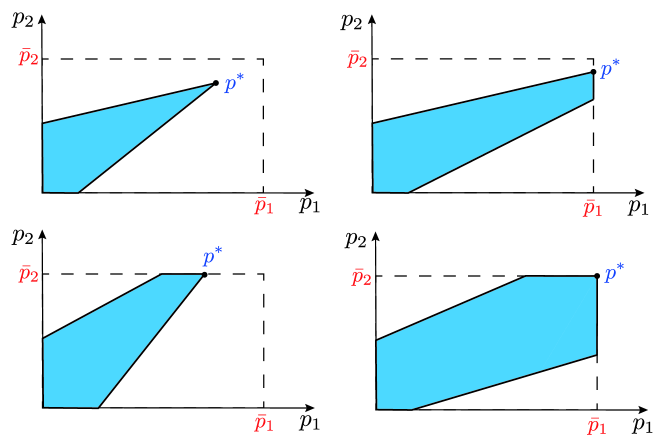
Figure 1: Examples of the possible shapes of ${\cal D}$ and the dominant clearing vector in the case of two nodes.

Lemma 4.3 implies that a clearing vector can be found by solving the following convex QP problem

$$\min_{p\in{{\mathbb{R}}^{n}}} \|\bar{\phi}^{{\mathrm{in}}}-\phi^{{\mathrm{in}}}\|_{2}^{2}$$ (9)

s.t.: $$\bar{p}\geq p\geq 0$$

$$c+A^{\top}p\geq p,$$

where $\phi^{{\mathrm{in}}}=c+A^{\top}p$, $\bar{\phi}^{{\mathrm{in}}}=\bar{c}+A^{\top}\bar{p}$. Alternatively, one may solve the LP program

$$\min_{p\in{{\mathbb{R}}^{n}}} \sum_{i=1}^{n}(\bar{\phi}^{{\mathrm{in}}}_{i}-\phi^{{\mathrm{in}}}_{i})$$ (10)

s.t.: $$\bar{p}\geq p\geq 0$$

$$c+A^{\top}p\geq p.$$

It can indeed be easily shown that both $\|\phi^{{\mathrm{in}}}-\bar{\phi}^{{\mathrm{in}}}\|_{2}^{2}$ and $\|\phi^{{\mathrm{in}}}-\bar{\phi}^{{\mathrm{in}}}\|_{1}={\mathbf{1}}^{\top}(\bar{\phi}^{{\mathrm{in}}}-\phi^{{\mathrm{in}}})$ are decreasing on $[0,\bar{p}]$. Hence, a unique minimizer $p=p^{*}$ exists in the optimization problems (9) and (10). Notice that usually uniqueness of a solution is guaranteed only for strictly convex function, whereas the linear function (10) is not strictly convex, and the function (9) fails to be strictly convex if $\det A=0$.

Whereas the dominant clearing vector $p^{*}$ depends on matrix $A$ and vectors $c,\bar{p}$, and the closed-form analytic expressions for its elements are not available, some properties of this clearing vector in fact do not depend on the liability matrix and are determined only by the topology of graph ${\cal G}$. In particular, the following lemma can be proved (see the appendix Section 8 for its proof) establishing the criterion for positivity of the dominant clearing vector’s elements.

Lemma 4.4

The element $p_{i}^{*}$ of the dominant clearing vector is positive if and only if $i$ is not a sink node ($\bar{p}_{i}>0$) and at least one of the following conditions holds:

1. $i$ has outside assets, that is, $c_{i}>0$;

2. $i$ is reachable from some node $j\neq i$ with $c_{j}>0$;

3. the strongly connected component of graph ${\cal G}$ to which $i$ belongs is a sink component.

4.2 Uniqueness of the clearing vector: a sufficient condition

In this subsection, we offer a sufficient condition ensuring that the dominant clearing vector $p^{*}$ is the unique clearing vector. In fact, we show that some elements of the clearing vector are always determined uniquely.

We start with introducing some auxiliary notation. Let $C^{+}\doteq\{i:c_{i}>0\}$ stand for the set of nodes that receive nonzero outside assets, and let $S\doteq\{i:\bar{p}_{i}=0\}$ stand for the set of sink nodes that owe no liability payments. We introduce the set

$$I_{0}\doteq C^{+}\cup S=\{i:c_{i}>0\lor\bar{p}_{i}=0\}.$$ (11)

The following lemma, whose proof is given in the appendix Section 8, establishes a sufficient condition for uniqueness of the clearing vector and generalizes results from [4, 18, 7].

Lemma 4.5

Let $I_{0}^{\prime}\supseteq I_{0}$ stand for the set of all nodes in the graph ${\cal G}$, from where $I_{0}$ can be reached. Then, for every clearing vector $p$ we have $p_{i}=p_{i}^{*}\quad\forall i\in I_{0}^{\prime}.$ In particular, if set $I_{0}$ is globally reachable in the graph of a financial network ${\cal G}$, then the dominant clearing vector $p^{*}$ is the only clearing vector corresponding to the vector of outside assets $c$.

Remark 4.6

Since each path in the graph ends in one of the sink components, it can be easily proved that the condition from Lemma 4.5 admits the following equivalent reformulation: each sink component of graph ${\cal G}$ is either trivial (contains only one node) or contains node $i$ such that $c_{i}>0$.

4.3 Uniqueness of the clearing vector: the general case

In this subsection we derive two necessary and sufficient criteria of the clearing vector’s uniqueness. The first of them (Theorem 4.7) assumes that the dominant clearing vector $p^{*}$ has been found. In this situation, one can describe the whole polytope of such vectors. If one is interested only in the uniqueness of a clearing vector, a simpler graph-theoretic criterion can be used (Theorem 4.10) that does not require to know $p^{*}$.

Assume that the condition in Lemma 4.5 does not hold, that is, $I_{0}^{\prime}\neq{\cal V}$. The banks corresponding to nodes from ${\cal V}_{1}\doteq{\cal V}\setminus I_{0}^{\prime}$ do not have outside assets (${\cal V}_{1}\cap C^{+}=\emptyset$) and do not pay to nodes from $I_{0}^{\prime}$ (otherwise, a chain of liability from them to $I_{0}$ would exist). Hence, matrix $A^{1}\doteq(a_{ij})_{i,j\in{\cal V}_{1}}$ is stochastic. At the same time, nodes from $I_{0}^{\prime}$ can have liability payments to nodes from ${\cal V}_{1}$, which depend only on the dominant vector $p^{*}$ and constitute the vector

$$c^{(1)}\doteq(c^{(1)}_{i})_{i\in{\cal V}_{1}},\quad c^{(1)}_{i}=c^{(1)}_{i}(p^{*})\doteq\sum_{k\in I_{0}^{\prime}}a_{ki}p_{k}^{*},\quad i\in{\cal V}_{1}.$$

We can now apply Lemma 4.5 to a reduced financial network ${\cal G}_{1}$ with node set ${\cal V}_{1}$, normalized payment matrix $A_{1}$ and vector of external assets $c^{(1)}$. Introducing the set

$$I_{1}=\{i\in{\cal V}_{1}:c_{i}^{(1)}>0\}$$

and denoting $I_{1}^{\prime}\supseteq I_{1}$ all nodes from which set $I_{1}$ is reachable (banks that are connected by chains of liability to nodes from $I_{1}$), Lemma 4.5 ensures that the elements of the reduced network’s clearing vector $p_{i},i\in I_{1}^{\prime}$, are determined uniquely. The definition (6) entails that if $p$ is a clearing vector for the original network, then its subvector $p^{1}=(p_{i})_{i\in{\cal V}_{1}}$ is a clearing vector for the reduced network ${\cal G}_{1}$. This also applies to $p^{*}$. Lemma 4.5 entails now that for each clearing vector $p$ (in the original network) one has $p_{i}=p_{i}^{*}\,\forall i\in I_{1}^{\prime}$.

If $I_{0}^{\prime}\cup I_{1}^{\prime}={\cal V}$, we have uniqueness of the clearing vector. Otherwise, we have a group of banks ${\cal V}_{2}={\cal V}\setminus(I_{0}^{\prime}\cup I_{1}^{\prime})$ that are not in debt to the nodes from $I_{1}^{\prime}$ and $I_{0}^{\prime}$, however, they can receive liability payments from the group $I_{1}^{\prime}$. For group ${\cal V}_{2}$, these payments may be treated as outside assets. Let

$$c^{(2)}\doteq(c_{i}^{(2)})_{i\in{\cal V}_{2}},\quad c_{i}^{(2)}\doteq\sum_{k\in I_{1}}a_{ki}p_{i}^{*}.$$

If the set $I_{2}=\{i\in{\cal V}_{2}:c_{i}^{(2)}>0\}$ is non-empty, one can consider the set $I_{2}^{\prime}\supseteq I_{2}$ of all nodes from where $I_{2}$ can be reached. Lemma 1 implies that the elements $p_{i},\,,i\in I_{2}^{\prime}$ of the clearing vector are uniquely determined: $p_{i}=p_{i}^{*}\,\forall i\in I_{2}^{\prime}$.

We arrive at the following iterative procedure, which allows to test the clearing vector’s uniqueness (and, in fact, even to find the whole set of clearing vectors).

Algorithm 1 Clearing vector’s uniqueness test.

Initialization. Compute the dominant clearing vector $p^{*}$ (e.g., by solving the LP (9)). Set $q\leftarrow 0$, $I_{0}\leftarrow C^{+}\cup S=\{i:c_{i}>0\lor\bar{p}_{i}=0\}$. Find the set $I_{0}^{\prime}\supseteq I_{0}$ of all nodes, from which $I_{0}$ is reachable.

repeat

     1) $q\leftarrow q+1$;

     2) ${\cal V}_{q}\leftarrow{\cal V}\setminus(I_{0}^{\prime}\cup I_{1}\ldots\cup I_{q-1}^{\prime})$;

     3) compute the vector of payments from $I_{q-1}^{\prime}$ to ${\cal V}_{q}$

$$c^{(q)}=(c^{(q)}_{i})_{i\in{\cal V}_{q}},\quad c^{(q)}_{i}\doteq\sum_{k\in I_{q-1}^{\prime}}a_{ki}p_{k}^{*}\quad\forall i\in{\cal V}_{q};$$

     4) find the set $I_{q}=\{i\in{\cal V}_{q}:c^{(q)}_{i}>0\}$;

     5) find the set $I_{q}^{\prime}\supseteq I_{q}$ of nodes from ${\cal V}_{q}$, from where $I_{q}$ can be reached in ${\cal G}$.

until ${\cal V}_{q}=\emptyset$ or $c^{(q)}=0$.

Theorem 4.7

Algorithm 1 stops after a finite number of steps $s\geq 0$. The elements of a clearing vector, corresponding to indices $i\in I_{0}^{\prime}\cup I_{1}^{\prime}\cup\ldots\cup I_{s}^{\prime}$, are uniquely determined: $p_{i}=p_{i}^{*}$. The clearing vector is unique if and only if ${\cal V}_{s}=\emptyset$, otherwise, there are infinitely many clearing vectors. Precisely, $p$ is a clearing vector if and only if

$$p_{i}=\begin{cases}p_{i}^{*},\quad i\in I_{0}^{\prime}\cup I_{1}\ldots\cup I_{s}^{\prime},\\ \xi_{i},\quad i\in{\cal V}_{s},\end{cases}$$ (12)

where $\xi\in{{\mathbb{R}}^{{\cal V}_{s}}}$ is an arbitrary vector satisfying the constraints

$$B^{\top}\xi=\xi,\quad 0\leq\xi_{i}\leq\bar{p}_{i}\,\forall i\in{\cal V}_{s},\quad B\doteq(a_{ij})_{i,j\in{\cal V}_{s}}.$$ (13)

A proof of Theorem 4.7 is offered in the appendix Section 8.

Example 4.8

Algorithm 1 is illustrated by Fig. 2, which displays a network with $n=15$ nodes that contains only one sink node ($S=\{0\}$) and three nodes with outside assets ($C^{+}=\{1,2,3$}), which together form the set $I_{0}$. Lemma 4.4 entails that in this situation $p_{i}^{*}>0$, $\forall i\neq 0,9$ (notice that nodes 13-15 constitute a sink component, satisfying thus condition 3) from Lemma 4.4). The set $I_{0}^{\prime}$ contains $I_{0}$ and two nodes $4,5$ that have liabilities towards nodes $0$ and $2$. The set $I_{1}$ contains nodes that have no liability to $I_{0}^{\prime}$, however, should receive payments from 4 and 5. Hence, $c^{(1)}_{6},c^{(1)}_{7},c^{(1)}_{8}>0$. The nodes $6,7,8$ constitute the set $I_{1}$; the set $I_{1}^{\prime}$ is obtained by adding node $9$ who has liability to one of them. On the next iteration of the algorithm, one computes the sets $I_{2}=\{10,11\}$ and $I_{2}^{\prime}=\{12\}\cup I_{2}$. The next vector $c^{(3)}$ will be zero, because the remaining nodes of the graph constitute an isolated group. Hence, the clearing vector is not unique, and for each clearing vector $p$ one has $p_{i}=p_{i}^{*}$, $\forall i=0,\ldots,12$.

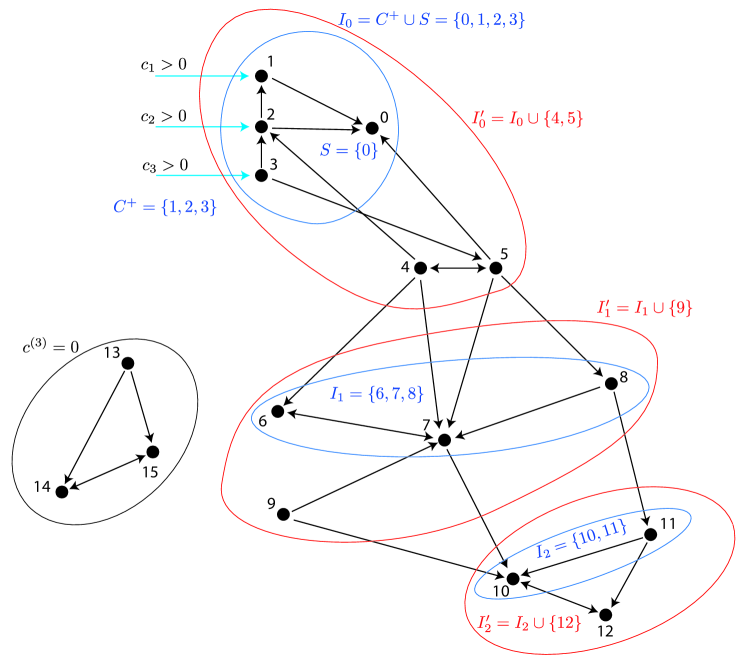
Figure 2: The sets $I_{s}$ (encircled by blue lines) and $I_{s}^{\prime}$ (encircled by red lines) for a special financial network with $n=15$ nodes with $p^{*}_{i}>0\,\forall i\neq 0$.

Theorem 4.7 entails the following technical proposition, which is of independent interest. The net vector (or the vector of equities) corresponding to the clearing vector $p$ is

$$\zeta\doteq\phi^{{\mathrm{in}}}-\phi^{{\mathrm{out}}}=c+A^{\top}p-p=\max(c+A^{\top}p-\bar{p},0)\geq 0.$$ (14)

The component $\zeta_{i}$ represents the net worth of node $i$, that is, the difference between the in- and the out-flows at that node.

Corollary 4.9

[4, 8] The vector of equities $\zeta$ is same for all possible clearing vectors $p$.

The proof of Corollary 4.9 is straightforward from the representation (12). Indeed, the equities of banks from ${\cal V}_{s}$ are all zeros, whereas the remaining equities depend only on the subvector $(p_{i})_{i\in I_{0}^{\prime}\cup\ldots\cup I_{s}^{\prime}}$, which is uniquely determined by $p^{*}=p^{*}(c,A,\bar{p})$.∎

Notice that although the subvector $\xi$ in (12) is defined non-uniquely, some of its elements are in fact uniquely determined due to Lemma 4.4. As we know, $\xi_{i}=p_{i}^{*}=0$ whenever $i$ does not belong to a sink component and is not reachable from $C^{+}$. Combining Theorem 4.7 with Lemma 4.4, we can establish an alternative uniqueness criterion, which does not require knowledge of the vector $p^{*}$.

Theorem 4.10

The following two conditions are equivalent:

1. the clearing vector is unique;

2. each non-trivial sink component of ${\cal G}$ either has a node from $C^{+}$ or is reachable from $C^{+}$.

A proof of Theorem 4.10 is given in the appendix Section 8.

4.4 Dicussion: Lemma 4.5 and Theorems 4.7 and 4.10 vs. previously known results

Comparing Theorem 4.7 to previously known results, several relevant features can be noticed. To find the dominant clearing vector $p^{*}$, one needs to know the matrix $\bar{P}$ (or, equivalently, $\bar{p}$ and $A$) and the vector of external assets $c\geq 0$. As we have already discussed, efficient algorithms do exist for computing this vector (e.g., by solving an LP or a convex QP). The computation of the sets $I_{s},I_{s}^{\prime},{\cal V}_{s}$ requires in fact very limited information. We do not need to compute the vectors $c^{(q)}$, it suffices to know which of their components are positive. A closer look at our algorithm shows that this depends on the set $C^{+}$ (nodes who receive external asset and the topology of graph ${\cal G}$ (which determines, in view of Lemma 4.4, which elements of $p^{*}$ are positive). This information allows us to check the uniqueness of the clearing vector and, furthermore, to find the components shared by all clearing vectors. Also, we give an explicit and simple description of all clearing vectors.

4.4.1 Criteria from [4] and [7]

The uniqueness criterion from [4] states that the clearing vector is unique if the set $C^{+}$ is globally reachable, being thus a special case of Lemma 4.5. The proof of this criterion (found first in [4] and simplified in [8]) starts with a direct proof of Corollary 4.9. An advantage of the approach developed in [4] is the possibility to generalize the proof (with some variations) to some advanced models of systemic risk [8, 20].

The criterion from [7] can be considered as another special case of Lemma 4.5; it also follows from the last statement of Lemma 4.3. This criterion guarantees uniqueness in the situation where all nodes are connected to the external sector by chains of liabilities.

It should be noted that, contrary to the present work, the aforementioned results from [4, 8, 7] do not allow to parameterize all clearing vectors when the uniqueness fails to hold.

4.4.2 An extension of the Eisenberg-Noe model and the uniqueness criterion from [23, 19]

In our current model, in the line of the original Eisenberg-Noe model, we represent payments to the external sector as payments to a fictitious node in the network. As such, these payments are subject to the same pro-rata rule that holds for all other nodes, i.e., they enjoy no priority in case of default. Some authors consider instead a situation in which some of the external payments (e.g., operational costs) cannot be reduced in spite of the dropping outside assets. In this situation, the non-negative vector $c\geq 0$ is replaced by the real vector $e\in\mathbb{R}^{{\cal V}}$ whose elements can be both positive and negative. Such a model, extending the original model from [4], was proposed in [20]. It should be noticed that, unlike the case where $e\geq 0$, a bank can become insolvent, i.e.

$$\zeta_{i}=(A^{\top}p)_{i}+e_{i}-p_{i}<0.$$

To take this effect into account, the definition of the clearing vector has to be modified to [20]:

$$p=\min(\bar{p},\max(A^{\top}p+e,0)).$$ (15)

Clearly, in the case where $e=c\geq 0$, the definition of the clearing vector (15) is equivalent to (6). It should be noted that the criteria earlier established in [23] (see also [24]) for testing the uniqueness of the solution of (15) are restricted to strongly connected networks (which excludes, in particular, the possibility of having sink nodes) and are thus inapplicable to the general Eisenberg-Noe model.

To the best of the authors’ knowledge, the only criterion allowing to test the uniqueness of clearing vectors in the general situation has been obtained in the very recent work [19]. Unlike Theorems 4.7 and 4.10, the criterion of  [19] is applicable to the situation where $e$ is not sign constrained. At the same time, in the situation of $e\geq 0$ this criterion appears to be superfluous and more computationally demanding than our results, because it requires to find not only the irreducible decomposition of matrix $A$ (equivalently, the structure of all strongly connected components in the graph), but also to compute the left and right Perron-Frobenius eigenvector for each irreducible block. These eigenvectors, needed for checking of the clearing vector’s uniqueness and to parameterize the whole set of such vectors, are not used in our criteria of the uniqueness.

5 Lifting the pro-rata condition

In this section we propose a new clearing mechanism that does not hinge upon the proportional payments rule. Without the pro-rata constraint in place, we have potentially more freedom to appropriately select a payment matrix $P$ that satisfies the conditions of Definition 3.1. These conditions do not identify the payment matrix univocally. Indeed, as we discussed extensively in the previous sections, one matrix that satisfies the definition is the one resulting from the pro-rata rule, but this may not be the only one, in general. This fact gives us some degrees of freedom that shall be used towards seeking clearing matrices who promote a virtuous behavior of the whole network. As it will be shown in Section 6, the proposed non-proportional clearing mechanism not only visibly reduces the overall total imbalance between the nominal and actual payments, but it also helps isolating defaults and preventing their cascaded spread over the network.

5.1 Optimal clearings

We next present an optimization-based approach for determining a clearing matrix that minimizes an appropriate system-level loss function. Recalling that $[0,\bar{P}]=\{P\in{{\mathbb{R}}^{n\times n}}:0\leq P\leq\bar{P}\}$, we consider the convex polyhedron in the space of matrices

$${\cal D}_{n\times n}=[0,\bar{P}]\cap\{P\in{{\mathbb{R}}^{n\times n}}:c+P^{\top}{\mathbf{1}}\geq P{\mathbf{1}}\}.$$

We call a function $F:[0,\bar{P}]\to{{\mathbb{R}}}$ decreasing if $F(P_{1})>F(P_{2})$ whenever $P_{1}\lneq P_{2}$. For any such function, consider the optimization problem

$$\min F(P)\quad\text{subject to}\quad P\in{\cal D}_{n\times n}.$$ (16)

The following result holds; see Section 8 in the Appendix for a proof.

Lemma 5.1

For any decreasing function $F:[0,\bar{P}]\to{{\mathbb{R}}}$, every local minimizer in problem (16) is a clearing matrix (as defined in Definition 3.1).

Notice that Lemma 5.1 does not require the function to be continuous. For a continuous function, the global minimum always exists due to compactness of $\mathcal{D}_{n\times n}$. Two examples of functions that are continuous and decreasing on $[0,\bar{P}]$ are

$$F_{1}(P)\doteq\|\bar{P}-P\|_{1} = \sum_{i,j=1}^{n}|\bar{P}_{ij}-P_{ij}|,$$ (17)

$$F_{2}(P)\doteq\|\bar{P}-P\|_{2}^{2} = \sum_{i,j=1}^{n}(\bar{P}_{ij}-P_{ij})^{2}.$$ (18)

Both these functions provide a global, system-level, measure of the impact of defaults on the deviation of payments from their nominal liabilities. In particular, minimization of the performance index (17) is equivalent to the problem

$$F_{1}^{*}=\min_{P\in{{\mathbb{R}}^{n,n}}} \|\bar{P}-P\|_{1}$$ (19)

s.t.: $$\bar{P}\geq P\geq 0$$

$$c+P^{\top}{\mathbf{1}}-P{\mathbf{1}}\geq 0,$$

which can be readily recast in the form of an LP, whereas minimization of (18) leads to the convex QP problem

$$F_{2}^{*}=\min_{P\in{{\mathbb{R}}^{n,n}}} \|\bar{P}-P\|_{2}^{2}$$ (20)

s.t.: $$\bar{P}\geq P\geq 0$$

$$c+P^{\top}{\mathbf{1}}-P{\mathbf{1}}\geq 0.$$

While both (19) and (20) are valid ways for obtaining a clearing matrix $P$, from the financial point of view they have different characteristics. Notice in fact that the objective in (20) is strongly convex, so the optimal clearing matrix resulting from (20) is unique. However, the $F_{2}$ criterion is expressed in “squared currency,” which may not have an immediate financial meaning. Further, this sum-of-squared losses function tends to avoid large individual losses, at the expense of possibly having many small losses. This is a well-known behavior of squared losses, but in the present context it may be critical since default is an on/off process: a node goes into default as soon as its balance goes negative, irrespective of how large is the negative balance. Especially for this reason our focus in this work is on the $F_{1}$ criterion in (19). As it is widely known, this $\ell_{1}$-norm criterion tends to be less sensitive to large residuals and promotes solutions that are sparse. Sparsity, in our context, is a very desirable property, since a sparse residual matrix $\bar{P}-P$ means that many of its entries are zero, which in turn means that many nodes meet their liabilities and thus do not default. We next focus on the $F_{1}$ criterion, which represents the total sum that is lost due to defaults (notice that in the case of no defaults we have $F_{1}^{*}=0$).

5.2 Non-uniqueness of clearing matrices

In general, the set of clearing matrices defined via Definition 3.1 has more than one element. Further, this set has a non-trivial structure and fails to be a complete lattice. Lemma 4.3 does not retain its validity in the class of all admissible clearing matrices, in particular, there exists no maximal clearing matrix, as exemplified by the following.

Example 5.2

Consider a degenerate 3-node network whose nodes 1 and 2 are sinks ($\bar{p}_{1i}=0,\bar{p}_{2i}=0$, $\forall i$) and receive no outside assets ($c_{1}=c_{2}=0$), whereas node 3 receives outside asset $c_{3}>0$ and owes to both 1 and 2 ($\bar{p}_{31},\bar{p}_{32}>0$). A clearing matrix $P$ must then have the following structure

$$P=\begin{bmatrix}0&0&0\\ 0&0&0\\ p_{31}&p_{32}&0\end{bmatrix},\quad p_{31}\in[0,\bar{p}_{31}],\,p_{32}\in[0,\bar{p}_{32}].$$ (21)

and equation (3) is equivalent to

$$p_{31}+p_{32}=\theta\doteq\min(\bar{p}_{31}+\bar{p}_{32},c_{3}).$$ (22)

Considering two clearing matrices

$$P_{1}=\begin{bmatrix}0&0&0\\ 0&0&0\\ \theta&0&0\end{bmatrix},\quad P_{2}=\begin{bmatrix}0&0&0\\ 0&0&0\\ 0&\theta&0\end{bmatrix},$$

one may easily notice that no matrix $P\geq\max(P_{1},P_{2})$ can satisfy (22). In particular, the set of clearing matrices understood in the sense of Definition 3.1 has no maximal element. It can be easily verified that every matrix (21) that satisfies (22) is a global minimizer of problem (19). Hence, in spite of the strict monotonicity of the cost function in (19), the optimal solution to (19) is not unique. Contrary, if we introduce the proportionality rule, the unique (thanks to Lemma 4.5) clearing vector and the corresponding clearing matrix, result to be, respectively

$$p^{*}=(0,0,\theta)^{\top},\quad P^{*}=\begin{bmatrix}0&0&0\\ 0&0&0\\ \frac{\bar{p}_{31}\theta}{\bar{p}_{31}+\bar{p}_{32}}&\frac{\bar{p}_{32}\theta}{\bar{p}_{31}+\bar{p}_{32}}&0\end{bmatrix}.$$

5.3 A two-stage approach for uniqueness

Given a liability matrix $\bar{P}$ and an in-flow vector $c\geq 0$ our purpose is to establish a policy that permits to determine uniquely a clearing matrix that globally minimizes the system-level loss $F_{1}$. Uniqueness is important since the clearing payments must be non controversial, and each player must be in condition to compute and agree univocally on the same payment values. As we discussed in the previous section, however, the LP problem in (19) may have multiple global optimal solutions, in general. The following lemma characterizes all optimal solutions to (19).

Lemma 5.3

Let $P^{*}$ be an optimal solution of problem (19). Then, the set of all optimal solutions to (19) is characterized as the polytope

$${\cal S}^{*}\doteq\{\tilde{P}=P^{*}+\Delta:\;0\leq\tilde{P}\leq\bar{P},\,c+\tilde{P}^{\top}{\mathbf{1}}-\tilde{P}{\mathbf{1}}\geq 0,\,{\mathbf{1}}^{\top}\Delta{\mathbf{1}}=0\}.$$

A proof of Lemma 5.3 is given in the appendix Section 8.

The next proposition illustrates how we can break the tie and specify a two-stage rule that results in a unique optimal clearing policy.

Proposition 5.4

Let $P^{*}$ be an optimal solution of problem (19), and let $F_{1}^{*}$ be the corresponding globally optimal loss level. Let further $\Delta^{*}$ be such that

$$\Delta^{*}=\arg\min_{\Delta\in{{\mathbb{R}}^{n,n}}} \|P^{*}+\Delta\|_{2}^{2}$$ (23)

s.t.: $$\bar{P}\geq P^{*}+\Delta\geq 0$$

$$c+(P^{*}+\Delta)^{\top}{\mathbf{1}}-(P^{*}+\Delta){\mathbf{1}}\geq 0$$

$${\mathbf{1}}^{\top}\Delta{\mathbf{1}}=0.$$

Then:

• $\tilde{P}^{*}\doteq P^{*}+\Delta^{*}$ is a clearing matrix;

• $\tilde{P}^{*}$ achieves the globally optimal loss level $F_{1}^{*}$, that is $F_{1}(\tilde{P}^{*})=F_{1}^{*}$;

• $\tilde{P}^{*}$ is the unique smallest-Euclidean-norm solution among all optimal solutions to (19).

A proof of Proposition 5.4 is given in the appendix Section 8.

We call this a two-stage approach for determining the unique optimal clearing matrix, since the method consists in solving two convex problems in sequence: first we solve the LP (19) and find any optimal solution $P^{*}$. Next, we solve the convex QP (23) and find its unique optimal $\Delta^{*}$. Finally, our optimal clearing matrix of interest is $\tilde{P}^{*}=P^{*}+\Delta^{*}$, which is the minimum norm solution among all possible optimal solutions to problem (19).

6 Numerical Experiments

We next evaluate numerically the systemic improvement of the optimal matrix clearings (i.e., those computed according to Proposition 5.4) with respect to the standard pro-rated clearings (computed according to (10)). The improvement is evaluated both in terms of reduction of the systemic loss $F_{1}$ and in terms of containment of default contagion, as expressed by the percentage of defaulted nodes in the network. First, we propose in Section 6.1 a simple schematic example, and then we perform extensive randomized tests in Section 6.2 using synthetic random networks similar to ones proposed in [21].

6.1 An illustrative schematic example

We consider a variation on the simplified network discussed in [7]. This network is composed of $n=5$ nodes (including the fictitious node representing the external sector), with liability matrix

$$\bar{P}=\left[\begin{array}[]{ccccc}0&180&0&0&180\\ 0&0&100&0&100\\ 90&0&0&100&50\\ 150&0&0&0&150\\ 0&0&0&0&0\end{array}\right],$$

where the last row refers to the fictitious node. Suppose there is a nominal scenario where external cash flows are given as

$$c=c_{{\mathrm{nom}}}\doteq[121,\;21,\;150,\;204,\;0]^{\top}.$$

It can be readily verified that in the nominal scenario all the nodes in the network remain solvent (no defaults), and the clearing payments coincide with the nominal liabilities. Consider next a situation in which a “shock” happens on the inflow at node $3$, so that this inflow reduces from $150$ to $120$, that is

$$c=c_{{\mathrm{shock}}}\doteq[121,\;21,\;130,\;204,\;0]^{\top}.$$

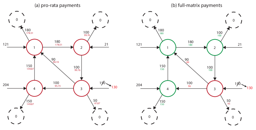
Figure 3: A four-nodes network with a shock on the cash inflow at node 3. Panel (a) shows the pro-rated clearing payments, panel (b) shows the optimal matrix clearings.

Under the pro-rata rule, the (unique) clearing payments, resulting from the solution of (10), are shown in smaller font below the nominal liabilities in the left panel of Figure 3: all nodes in the network default in a cascade fashion due to initial default of node $3$. The total defaulted amount, defined as the sum of all the unpaid liabilities is in this case $F_{1}=13.98$.

Then, we lifted the pro-rata rule, and we computed the unique clearing payments according to Proposition 5.4. The results in this case are shown in the right panel of Figure 3: only node $3$ defaults, while all other nodes manage to pay their full liabilities. Not only we reduced the sum of all unpaid liabilities to $F_{1}=10$, but we also obtained isolation of the contagion, since the default is now limited to node $3$ and did not spread to other parts of the network.

6.2 Random networks test

The random graphs used for simulations are constructed using a technique inspired by [21]. The topology of the graph is given by the standard Erdös-Renyi $\cal{G}(n,p)$ graph. The interbank liabilities $\bar{P}_{ij}$ for every edge $(i,j)$ of the random graph are then found by sampling from a uniform distribution $\bar{P}_{ij}\sim\mathcal{U}(0,P_{max})$, where $P_{max}$ is the maximum possible value of a single interbank payment. In the experiments we set $P_{max}=100$. Unlike [21], the values $\bar{P}_{ij}$ can thus be heterogeneous. Also, we do not consider payments to external sector (deposits etc.): as it has been discussed, we can always get rid of them by introducing a fictitious node.

Following [21], we define the total amount of the external assets $E=\frac{\beta}{1-\beta}I$, where $I=\sum_{i,j=1}^{n}\bar{P}_{ij}$ is the total amount of the interbank liabilities and $\beta=E/(E+I)$ is a parameter representing the percentage of external assets in total assets at the system level; in our experiments $\beta=0.05$. The nominal asset vector $\bar{c}$ is then computed in two steps. First, each bank is given the minimal value of external assets under which its balance sheet is equal to zero. At the second step, the remainder of the aggregated external assets is evenly distributed among all banks.

The financial shock is modeled by randomly choosing a subset of $n_{s}$ banks of the system and nullifying their external financial assets.

6.2.1 A numerical study of the “price” of proportionality

To evaluate the “price” of imposing the pro-rata rule, we consider the $F_{1}$ performance index presented in (17). This is used as system loss also in [7]. Its minimal value over all matrices obeying the pro-rata constraint (5) is $F_{1}^{(\mathrm{pr})}=\sum_{i}(\bar{p}_{i}-p_{i}^{*})$, where $p^{*}$ is the dominating clearing vector from Lemma 4.3, which is found by solving problem (9). Relaxing the pro-rata constraint, we use the two-stage approach presented in Sec. 5.3 to find the globally optimal clearing matrix $P^{*}$, resulting in the system loss $F_{1}^{(\mathrm{nopr})}=\|\bar{P}-P^{*}\|_{1}$. The price, or global effect, of the pro-rata rule can thus be estimated by the following ratio

$$G=\frac{F_{1}^{(\mathrm{pr})}-F_{1}^{(\mathrm{nopr})}}{F_{1}^{(\mathrm{pr})}}\in[0,1].$$

If $G=0$ (as, e.g., in Example 2, where all clearing matrices are optimal), the imposition of pro-rata constraint is “gratuitous” in the sense that it does not increase the aggregate system loss: $F_{1}^{(\mathrm{pr})}=F_{1}^{(\mathrm{nopr})}$. The larger value $G$ we obtain, the more “costful” is the pro-rata restriction.

It seems natural that $G$ is growing as the graph is becoming more dense, since in this situation the pro-rata rule visibly reduces the number of free variables in the optimization problem. We have tested this conjecture using the random model described above. The random graph contained $n=50$ nodes, whereas the average node degree $d=np$ varied from $0$ to $35$. The number $n_{s}$ of nodes that receive the shock varies from 1 to 5. The results were averaged over 50 runs. The resulting dependence between $G$ and $d$ is illustrated in Fig. 4. We can see that the relaxation of the pro-rata rule can give gain up to 43%. We can observe that, when there is a stronger shock, the relaxation of the pro-rata rule has a larger impact.

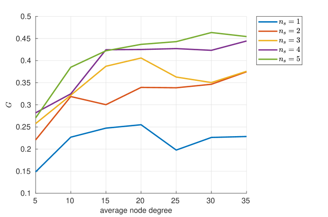
Figure 4: Gain obtained by relaxing the pro-rata rule.

To evaluate the price of the pro-rata rule, we also introduce another metric that measures the number of defaulted nodes. This metric evaluates the dimension of the failure cascade caused by the initial shock. Fig. 5 compares the number of defaulted nodes ($\phi^{{\mathrm{out}}}_{i}<\bar{\phi}^{{\mathrm{out}}}_{i}$) with or without the pro-rata rule. We observe that relaxing the pro-rata rule significantly reduces the failure cascade.

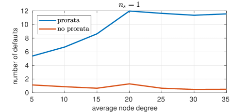
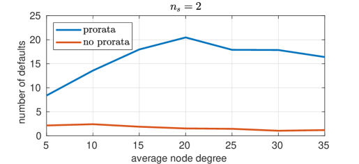
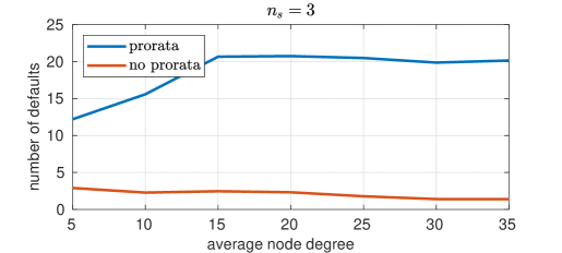
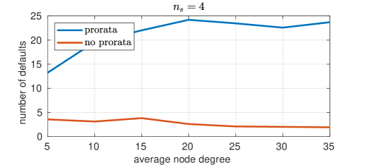
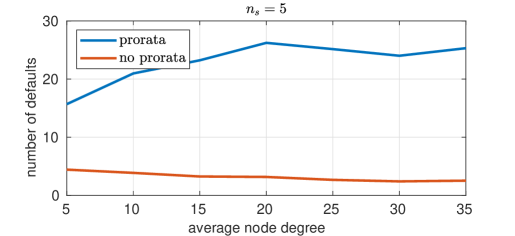
Figure 5: Numbers of defaulting nodes with or without the pro-rata rule.

7 Conclusions

Based on the financial networks model of [4], we explored in this paper the concept of a clearing vector of payments, and we developed new necessary and sufficient conditions for its uniqueness, together with a characterization of the set of all clearing vectors, see Theorem 4.7 and Theorem 4.10. Further, we examined matrices of clearing payments that naturally arise if one relaxes the pro-rata rule. Optimal clearing matrices can be computed efficiently by solving a convex optimization problem. Using numerical experiments with randomly generated synthetic networks, we showed that relaxation of the pro-rata rule allows to reduce significantly the overall systemic loss and the total number of defaulted nodes.

Many aspects remain to be explored. First and foremost, the biggest gap from theory to practice is that, in practice, the overall structure of the financial network is not know precisely, let alone the inter-bank liability amounts. For effective practical implementation, therefore, one should develop a system-level (i.e., global) approach whose iterations are based only on local exchange of information between nodes. The development of such distributed and decentralized optimal clearing payment algorithm is the subject of ongoing research. Another interesting aspect arises if one allows the liabilities to be spread over some interval of time, rather than cleared instantly, as it is supposed in the mainstream model of  [4]. This would lead to dynamic clearing payments, and to the ensuing optimal dynamic optimization problems. One discrete-time model of dynamic clearing payment is studied in our paper [25], which substantially exploits the theory developed in the present work, in particular, Lemma 4.3. Some other models, introducing quite complicated continuous-time dynamics, are available in the very recent works [26, 27, 28].

8 Appendix

8.1 Technical preliminaries

The proof of the main results of this paper are based on few technical propositions.

The following simple proposition follows, e.g., from [29, Corollary 4.3$a^{\prime}$]

Proposition 8.1

Each graph contains at least one sink strong component. Any node whose component is not a sink is a connected to one of the sink components by a path.

We will also use a technical lemma establishing necessary and sufficient conditions for the Schur stability of substochastic matrices. The spectral radius of a square matrix $A$ is denoted by $\rho(A)$. We call a matrix $A$ Schur stable if $\rho(A)<1$. The Gershgorin disk theorem implies that $\rho(A)\leq 1$ for any substochastic matrix $A$. If $A$ is stochastic, then $\rho(A)=1$ and $A$ cannot be Schur stable.

Lemma 8.2

Let $A\in{{\mathbb{R}}^{{\cal V}\times{\cal V}}}$ be a substochastic matrix. Then three statements are equivalent:

1. Matrix $A$ is Schur stable: $\rho(A)<1$;

2. Submatrix $A^{0}=(a_{i,j})_{i,j\in{\cal V}_{0}}$ is not stochastic for every subset of indices ${\cal V}_{0}\subseteq{\cal V}$;

3. The set of nodes ${\cal V}_{d}=\{i:\sum_{j}a_{ij}<1\}$ is non-empty and globally reachable in graph ${\cal G}[A]$;

4. Each strong component of ${\cal G}[A]$ being a sink contains at least one node from ${\cal V}_{d}$.

Proof 8.3

Proof of Lemma 8.2. Implication $3\Longrightarrow 1$ is a well-known fact, see e.g. [30, Lemma 7].

To prove 1)$\Longrightarrow$2) notice that if submatrix $A^{0}=(a_{i,j})_{i,j\in{\cal V}_{0}}$ is stochastic, then $0\leq\sum_{k\not\in{\cal V}_{0}}a_{ik}\leq 1-\sum_{j\in{\cal V}_{0}}a_{jk}=0\,\forall i\in{\cal V}_{0}$, that is, $a_{ik}=0\,\forall i\in{\cal V}_{0},k\not\in{\cal V}_{0}$. Hence, $A$ is decomposable as follows

$$A=\begin{pmatrix}A^{0}&\mathbf{O}\\ *&*\end{pmatrix},$$ (24)

where $\mathbf{O}$ is a block of zeros and $*$ stand for some other submatrices. Hence, $1$ is an eigenvalue of $A$, in particular, $\rho(A)=1$ and $A$ is not Schur stable.

Implication 2$\Longrightarrow$4 is straightforward from the definition of a sink component. If ${\cal V}_{0}$ is the set of nodes belonging to such a strong component, then matrix $A$ is decomposed as in (24), where $A^{0}=(a_{i,j})_{i,j\in{\cal V}_{0}}$. In view of statement 2, $A^{0}$ is not a stochastic matrix, so the sum in at least one of its rows is less than $1$, that is, ${\cal V}_{0}\cap{\cal V}_{d}\neq\emptyset$.

Implication 3$\Longrightarrow$4 is straightforward from Proposition 8.1 and the definition of a strongly connected component (whose every two nodes are mutually reachable).∎

8.2 Proofs of the main results

Proof 8.4

Proof of Lemma 4.3. Since ${\cal D}$ is compact (closed and bounded), the projection map $p\mapsto p_{i}$ reaches a maximal value $p_{i}^{*}=\max_{p\in{\cal D}}p_{i}$. The vector $p^{*}\doteq(p_{i}^{*})_{i\in{\cal V}}$, by construction, dominates every vector from ${\cal D}$. It remains to show that this vector belongs to ${\cal D}$. By definition, $p_{i}^{*}\in[0,\bar{p}_{i}]$, $\forall i$. Also, $c+A^{\top}p^{*}\geq c+A^{\top}p\geq p$, $\forall p\in{\cal D}$. Hence, for each index $i\in{\cal V}$ one has

$$(c+A^{\top}p^{*})_{i}\geq p_{i}\quad\forall p\in{\cal D}.$$

Taking the maximum over all $p$, one shows that

$$(c+A^{\top}p^{*})_{i}\geq p_{i}^{*}=\max_{p\in{\cal D}}p_{i},\;\forall i\in{\cal V},$$

i.e., $c+A^{\top}p^{*}\geq p^{*}$, finishing the proof of statement 1.

Statement 2 is now straightforward from Definition 4.2.

Statement 3 now follows from [4, Lemma 4], stating that every minimizer in problem (8) with a decreasing function $F$ is a clearing vector. We give here the proof for the reader’s convenience. Assume, by the purpose of contradiction, that (6) fails to hold, that is, $p_{i}^{*}<\min\left(\bar{p}_{i},c_{i}+\sum_{k\neq i}a_{ki}p_{k}^{*}\right)$ for some $i$. Consider the vector $\hat{p}\doteq p^{*}+\delta\mathbf{e}_{i}$, where $\delta>0$ is sufficiently small and $\mathbf{e}_{i}$ is the coordinate vector whose $i$th coordinate is $1$ and others are null. By noticing that $\left(c+A^{\top}\hat{p}\right)_{i}>\hat{p}_{i}$ and

$$\left(c+A^{\top}\hat{p}\right)_{j}\geq\left(c+A^{\top}p^{*}\right)_{j}\geq p_{j}^{*}=\hat{p}_{j}\quad\forall j\neq i,$$

one shows that $\hat{p}\in{\cal D}$, which contradicts Statement 1.

To prove statement 4, denote the set of nodes of a sink component by ${\cal V}_{0}$. Then, stochastic matrix $A$ decomposes as in (24), and submatrix $A^{0}=(a_{i,j})_{i,j\in{\cal V}_{0}}$ is also stochastic. Furthermore, this matrix is irreducible due to the definition of a strongly connected component. Thanks to the Perron-Frobenius theorem, $A^{\top}$ has a positive eigenvector $\pi^{0}$ such that $A^{\top}\pi^{0}=0$. Denoting

$$\pi_{i}=\pi_{i}^{0}\,\forall i\in{\cal V}_{0},\quad\pi_{i}=0\,\forall i\not\in{\cal V}_{0},$$

one obviously has $A^{\top}\pi=\pi$. Notice that vector $p^{\varepsilon}=p^{*}+\varepsilon\pi$ obeys the inequality $p^{\varepsilon}\leq c+A^{\top}p^{\varepsilon}$ for each $\varepsilon>0$ and, furthermore, $p^{\varepsilon}_{i}=p^{*}_{i}\leq\bar{p}_{i}\,\forall i\not\in{\cal V}_{0}$. Since $p^{*}$ is the maximal element in ${\cal D}$, $p^{\varepsilon}\not\in{\cal D}\,\forall\varepsilon>0$, which is possible only when $p^{*}_{i}=\bar{p}_{i}$ for some $i\in{\cal V}_{0}$.

Statement 5 follows from Lemma 8.2 and the maximality of $p^{*}$. Let $p$ be a clearing vector enjoying the property from statement 4 and $I=\{i:p_{i}=\bar{p}_{i}\}$. Notice that, in view of Proposition 8.1, the set $I$ is globally reachable in graph ${\cal G}[A]$ (each node is connected to a sink strong component, and all nodes within this component are connected to some node from $I$). Denoting $I^{c}={\cal V}\setminus I$, submatrix $\hat{A}=(a_{ij})_{i,j\in I^{c}}$, obviously, cannot contain stochastic submatrices, being thus Schur stable (Lemma 8.2). The corresponding subvector $\hat{p}=(p_{j})_{j\in I^{c}}$ obeys the equation

$$\hat{p}=\hat{A}^{\top}p+\hat{c},\quad\hat{c}_{j}\doteq c_{j}+\sum_{i\in I}a_{ij}\bar{p}_{i}\,\forall j\in I^{c}.$$ (25)

Recalling that $p^{*}\geq p$, one has $p_{i}^{*}=\bar{p}_{i}\,\forall i\in I$; for this reason, subvector $\hat{p}^{*}=(p_{j}^{*})_{j\in I^{c}}$ also obeys (25), which means that $\hat{p}=\hat{p}^{*}$ and, therefore, $p=p^{*}$. ∎

Proof 8.5

Proof of Lemma 4.4. We start with “if” part. If $c_{i}>0$ and $\bar{p}_{i}>0$, then polytope ${\cal D}$, obviously, contains the vector $\varepsilon\mathbf{e}_{i}$, where $\varepsilon\in(0,\min(c_{i},\bar{p}_{i}))$. Since $p^{*}=\max{\cal D}$, we have $p_{i}^{*}>0$ whenever condition 1) holds. Notice also that if $p_{j}^{*}>0,p_{i}^{*}>0$ and $a_{ji}>0$, then (6) implies that $p_{i}^{*}>0$. Hence, condition 2) also entails that $p_{i}^{*}>0$. Assume now that condition 3) holds and let ${\cal I}$ be the set of nodes of the strongly connected component containing $i$. Since $i$ is not a sink, this component is non-trivial (contains two or more nodes), and for each $j\in{\cal I}$ we have $\bar{p}_{j}>0$. Also, the submatrix $\tilde{A}=(a_{jk})_{j,k\in{\cal I}}$ is stochastic and irreducible, hence, in view of the Perron-Frobenius theorem, there exist a strictly positive eigenvector $v\in\mathbb{R}^{{\cal I}}$ such that $A^{\top}v=v$. Rescaling, one may assume that $v_{i}\leq\bar{p}_{i}\,\forall i\in{\cal I}$. Hence, ${\cal D}$ contains the vector $p$, where

$$p_{j}\doteq\begin{cases}v_{j},j\in{\cal I}\\ 0,j\not\in{\cal I}\end{cases}\quad\forall j\in{\cal V},$$

in particular, $p_{i}^{*}\geq p_{i}>0$.

To prove the “only if” part, notice first that $p_{i}^{*}>0$ entails that $\bar{p}_{i}>0$, so $i$ is not a sink node. Assume, on the contrary, that none of 1)-3) holds. Consider again the strongly connected component ${\cal I}\ni i$ and the corresponding irreducible submatrix $\tilde{A}=(a_{jk})_{j,k\in{\cal I}}$. Since condition 3) is violated, we have $\rho\doteq\rho(\tilde{A})<1$. Introducing the positive Perron-Frobenius eigenvector $v\in{\cal I}$ such that $\tilde{A}^{\top}v=v$ and  (6) entails that

$$\begin{split}0<\sum_{j\in{\cal I}}v_{j}p_{j}^{*}\leq\sum_{j\in{\cal I}}v_{j}\sum_{k\in{\cal I}}a_{kj}p_{k}^{*}+\sum_{j\in{\cal I}}v_{j}\sum_{k\not\in{\cal I}}a_{kj}p_{k}^{*}\leq\\ \leq\rho\sum_{k\in{\cal I}}v_{k}p_{k}^{*}+\sum_{j\in{\cal I}}v_{j}\sum_{k\not\in{\cal I}}a_{kj}p_{k}^{*}.\end{split}$$

The latter inequality may hold only if $k\not\in{\cal I}$ exists such that $a_{kj}p_{k}^{*}>0$. In other words, there exists another strongly connected component ${\cal I}_{1}\neq{\cal I}$ such that $p_{j}^{*}>0\,\forall j\in{\cal I}_{1}$ and ${\cal I}_{1}$ is connected to ${\cal I}$ by at least one arc (this implies that no arc can go from ${\cal I}$ to ${\cal I}_{1}$). Since condition 2) is violated for $i$, conditions 1 and 2 are also violated for every $i_{1}\in{\cal I}_{1}$. Now we can repeat the argument, replacing ${\cal I}$ by ${\cal I}_{1}$ and find another strongly connected component ${\cal I}_{2}\neq{\cal I}_{1}$, such that at least one arc comes from ${\cal I}_{2}$ to ${\cal I}_{1}$ (in view of this ${\cal I}_{2}\neq{\cal I}$), $p_{j}^{*}>0\,\forall j\in{\cal I}_{2}$ and none element of ${\cal I}_{2}$ satisfies condition 1 or 2. Repeating this process, one could construct the infinite set of disjoint strongly connected components ${\cal I}_{0}\doteq{\cal I},{\cal I}_{1},{\cal I}_{2},\ldots$ such that ${\cal I}_{s}$ is connected to ${\cal I}_{s-1}$, $p_{j}^{*}>0\,\forall j\in{\cal I}_{s}$ yet conditions 1 and 2 fail to hold for $i\in{\cal I}_{s}$. This leads to the contradiction (the set of nodes ${\cal V}$ is finite). ∎

Proof 8.6

Proof of Lemma 4.5. Consider an arbitrary clearing vector $p^{0}$ and let $J\doteq\{i:p_{i}^{0}<\bar{p}_{i}\}$. Our goal is to show that $p^{0}_{i}=p^{*}_{i}\,\forall i\in I_{0}^{\prime}$.

Step 1. In view of (6), the vector $p=p^{0}$ obeys the equations

$$\begin{gathered}p_{i}=\bar{p}_{i}\quad\forall i\not\in J,\\ p_{i}=(c+A^{\top}p)_{i}=c_{i}+\sum_{k\not\in J}a_{ki}\bar{p}_{k}+\sum_{j\in J}a_{ji}p_{j}\;\forall i\in J.\end{gathered}$$ (26)

Step 2. We are going to show that if (26) has at least one solution, then $p=p^{*}$ should also be a solution to (26). Indeed, every solution to system (26) is a global minimizer in the optimization problem (8) with the objective function

$$F(p)\doteq\sum_{k\not\in J}(\bar{p}_{k}-p_{k})+\sum_{j\in J}\left(c_{j}+\sum_{i\in{\cal V}}a_{ij}p_{i}-p_{j}\right).$$ (27)

If $p^{0}$ satisfies (26), then $F(p^{0})=0\leq F(p)\,\forall p\in{\cal D}$. The function (27) is non increasing, because it can be written as

$$F(p)=\beta-b^{\top}p,\quad b_{i}\doteq 1-\sum_{j\in I}a_{ij}\geq 0,\quad\beta=\rm const,$$

Lemma 4.3 guarantees that $p^{*}$ is a global minimizer in (8), and hence $F(p^{*})=0$. Recalling that $p^{*}\in{\cal D}$, this is possible only if all addends in the right-hand side of (27) vanish as $p=p^{*}$.

Step 3. We now show that the equations (26) uniquely determine the subvector $(p_{i})_{i\in I_{0}^{\prime}}$. The first equation in (26) entails that $p_{i}=\bar{p}_{i}\,\forall i\in I_{0}^{\prime}\setminus J$. By construction, the set $I_{0}^{\prime}$ cannot be reached from any other node $j\not\in I_{0}^{\prime}$ (otherwise, $I_{0}$ could also be reached from $j$), that is, $a_{ji}=0$ whenever $i\in I_{0}^{\prime}$ and $j\not\in I_{0}^{\prime}$. Hence, for all solutions to (26) one has

$$p_{i}=c_{i}+\sum_{k\not\in J}a_{ki}\bar{p}_{k}+\sum_{j\in I_{0}^{\prime}\cap J}a_{ji}p_{j}\quad\forall i\in I_{0}^{\prime}\cap J.$$ (28)

We are now going to show that the matrix $\tilde{A}=(a_{ij})_{i,j\in I_{0}^{\prime}\cap J}$ is Schur stable. Assume, by purpose of contradiction , that $\tilde{A}$ is not Schur stable and thus (see Lemma 8.2) contains a stochastic submatrix $(a_{ij})_{i,j\in K}$, where $K\subseteq I_{0}^{\prime}\cap J$. Since $A$ is also stochastic, one has $a_{ij}=0\,\forall i\in K,j\in{\cal V}\setminus K$. Denoting

$$\ \tilde{z}\doteq(z_{i})_{i\in{\cal V}},\quad z_{i}\doteq\begin{cases}1,\,i\in K,\\ 0,\,i\not\in K,\end{cases}$$

one obviously has $Az\geq z$ or, equivalently, $z^{\top}A^{\top}\geq z^{\top}$. The second equation in (26) entails that

$$\begin{split}z^{\top}p=\sum_{i\in K}z_{i}p_{i}=\sum_{i\in K}z_{i}\left(c_{i}+\sum_{j\in{\cal V}}a_{ji}p_{j}\right)\overset{z_{i}=0\,\forall i\not\in K}{=\joinrel=\joinrel=\joinrel=}\\ =\sum_{i\in{\cal V}}z_{i}\left(c_{i}+\sum_{j\in{\cal V}}a_{ji}p_{j}\right)\geq z^{\top}c+z^{\top}p,\end{split}$$

whence $z^{\top}c=0$ and thus $K\cap C^{+}=\emptyset$. On the other hand, $K\subseteq J\subseteq{\cal V}\setminus S$, therefore, $K$ and $I_{0}$ are disjoint. By construction, graph ${\cal G}$ contains no arcs connecting $K$ to nodes from ${\cal V}\setminus K$, in particular, $I_{0}$ is not reachable from $K$. This contradicts to the definition of $I_{0}^{\prime}\supseteq K$. The contradiction shows that $\tilde{A}$ is Schur stable, in particular, (28) has a unique solution. Since both $p^{0}$ and $p^{*}$ satisfy (26) and (28), $p_{i}^{0}=p_{i}^{*}$ for all $i\in I_{0}^{\prime}$.∎

Proof 8.7

Proof of Theorem 4.7. The first statement is obvious, since the sets $I_{0}^{\prime},I_{1}^{\prime},\ldots$ are disjoint and the set of all nodes ${\cal V}$ is finite.

To prove the second statement, we show it via induction on $k=0,1,\ldots$ that for each clearing vector $p$ and each $k$ we have $p_{i}=p_{i}^{*}\,\forall i\in I_{k}^{\prime}$. The induction base ($k=0$) is proved in Lemma 4.5. Assume that the statement has been proved for $k=0,\ldots,q-1$ (where $q\geq 1$); we have to prove it for $k=q$. By construction, banks from ${\cal V}_{q}$ ($q\geq 1$) have no liability to banks from ${\cal V}\setminus{\cal V}_{q}=I_{0}^{\prime}\cup\ldots\cup I_{q-1}^{\prime}$. Also, they neither have outside assets ($c_{i}=0\,\forall i\not\in I_{0}$) nor receive payments from banks from $I_{0}^{\prime},\ldots,I_{q-2}^{\prime}$. Only banks from $I_{q-1}^{\prime}$ can pay liability to them. For each clearing vector $p$, (6) entails that

$$p_{i}=\min\left(\bar{p}_{i},\sum_{s\in I_{q-1}^{\prime}}a_{si}p_{s}+\sum_{k\in{\cal V}_{q}}a_{ki}p_{k}\right)\quad\forall i\in{\cal V}_{q}.$$ (29)

In view of the induction hypothesis, the first sum is nothing else than $c_{i}^{(q)}$ for all clearing vectors $p$. Hence, for any clearing vector $p$ (of the original financial network) the subvector $(p_{i})_{i\in{\cal V}_{q}}$ serves a clearing vector in the reduced financial network, determined by the set of nodes ${\cal V}_{q}\neq\emptyset$, the respective submatrix $A^{q}=(a_{ij})_{i,j\in{\cal V}_{q}}$ and the vector $c^{(q)}$, standing for the “external” assets. This holds, in particular, for the dominant clearing vector $p=p^{*}$. Lemma 4.5 guarantees that the elements $p_{i},i\in I_{q}^{\prime}$ are determined uniquely, that is, $p_{i}=p_{i}^{*}\,\forall i\in I_{q}^{\prime}$, which proves the induction step $k=q$. This finishes the proof of the second statement of Theorem 4.7.

Furthermore, it is now obvious that each clearing vector (that is, a solution to (6)) has the structure (12), where $\xi=(p_{i})_{i\in{\cal V}_{s}}\geq 0$ is some vector. If ${\cal V}_{s}=\emptyset$ (and the component $\xi$ is empty), the only clearing vector is $p=p^{*}$. Otherwise, $\xi$ obeys (13). Indeed, the matrix $B$ is stochastic by construction, so that ${\mathbf{1}}^{\top}B={\mathbf{1}}^{\top}$. In view of (6), one has

$$\xi\leq B^{\top}\xi.$$

Multiplying the latter inequality by ${\mathbf{1}}^{\top}$, one shows that it can only hold if $\xi=B^{\top}\xi$. On the other had, $\xi_{i}\leq\bar{p}_{i}\,\forall i\in{\cal V}_{s}$. The inverse statement is also obvious: each vector (12) satisfying (13) is a solution to (6). To finish the proof of the theorem, it remains to show that there are infinitely many subvectors $\xi$ obeying (13). Notice that $B$ is a stochastic matrix, and hence $\rho(B)=1$. Also, $\bar{p}_{i}>0\,\forall i\in{\cal V}_{s}$ (the nodes cannot be sinks). The Perron-Frobenius theorem entails the existence of at least one non-negative eigenvector $\xi^{0}\in{{\mathbb{R}}^{{\cal V}_{s}}}\setminus\{0\}$, which obeys (13). Obviously, the set of all vectors satisfying (13) is a convex polytope, which contains a trivial vector $\xi=0$ and, thus, also the whole line segment $[0,\xi^{0}]$. We have proved that the set of clearing vectors in infinite. ∎

Proof 8.8

Proof of Theorem 4.10. Suppose that (i) holds and consider some non-trivial sink component whose set of nodes is ${\cal I}$. Obviously, $\bar{p}_{i}>0\,\forall i\in{\cal I}$. The submatrix $\tilde{A}=(a_{ij})_{i,j\in{\cal I}}$ is stochastic, let $v\in\mathbb{R}^{{\cal I}}$ stand for the Perron-Frobenius eigenvector of $A^{\top}$ such that $A^{\top}v=v$. Assume that ${\cal I}$ neither intersects $C^{+}$ nor is reachable from $C^{+}$. If $j\not\in{\cal I}$ is connected to some node $i\in{\cal I}$, then $c_{j}=0$ and $j$ cannot be reached from $C^{+}$. In view of Lemma 4.4, $p_{j}^{*}=0$ and, therefore, for all vectors from ${\cal D}$ we have $p_{j}=0$. Therefore, every vector $p$ such that

$$p=\begin{cases}p_{i}^{*},i\not\in{\cal I},\\ \varepsilon v_{i},i\in{\cal I}\end{cases}$$

satisfies (6) when $\varepsilon>0$ is small enough. We arrive at the contradiction with the assumption of the clearing vector’s uniqueness. Implication (i)$\Longrightarrow$(ii) is proved.

Suppose now that (ii) holds yet the clearing vector is not unique. Consider the final set ${\cal V}_{s}\neq\emptyset$ found by Algorithm 1 ($s\geq 1$). By construction, no arc leads from ${\cal V}_{s}$ to $I_{0}^{\prime},\ldots,I_{s-1}^{\prime}$, therefore, ${\cal V}_{s}$ contains at least one sink component. This sink component cannot be trivial, because all sink nodes belong to $I_{0}\subseteq I_{0}^{\prime}$. For the same reason, this sink component contains no nodes from $C^{+}$. In view of (ii), a path from $C^{+}$ to ${\cal V}_{s}$ exists. In view of Lemma 4.4, for each node $j$ on this path we have $p_{j}^{*}>0$. Hence, there should exist an arc $j\to i$ connecting some $j\not\in{\cal V}_{s}$ (with $p_{j}^{*}>0$) to some $i\in{\cal V}_{s}$. This contradicts to the assumption that ${\cal V}_{s}$ is a final set, because $c^{(s)}>0$. Implication (ii)$\Longrightarrow$(i) is proved. ∎

Proof 8.9

Proof of Lemma 5.1. Assume, by the purpose of contradiction, that a local minimizer $P^{*}$ fails to satisfy (3). Hence, an index $i$ exists such that

$$p^{*}_{i}\doteq(P^{*}{\mathbf{1}})_{i}=\sum_{j}p_{ij}^{*}<\min\left(\bar{p}_{i},c_{i}+\sum_{k}p_{ki}^{*}\right).$$

Since $p^{*}_{i}<\bar{p}_{i}$, there exists some $j$ such that $p^{*}_{ij}<\bar{p}_{ij}$. Then for small $\delta>0$ matrix $\hat{P}=P^{*}+\delta\mathbf{e}_{i}\mathbf{e}_{j}^{\top}$ (obtained from $P^{*}$ by the replacement $p^{*}_{ij}\mapsto p^{*}_{ij}+\delta$, all other entries being invariant) belongs to ${\cal D}_{n\times n}$. Indeed, $\hat{P}\in[0,\bar{P}]$ and

$$\hat{p}\doteq\hat{P}{\mathbf{1}}=p^{*}+\delta\mathbf{e}_{i}\leq c+(P^{*})^{\top}{\mathbf{1}}\leq c+(\hat{P})^{\top}{\mathbf{1}}.$$

At the same time, $F(\hat{P})<F(P^{*})$. This contradicts to the assumption of local optimality. ∎

Proof 8.10

Proof of Lemma 5.3. The proof is immediate by observing that if $\tilde{P}$ is optimal for (19) then it must be that $F_{1}(\tilde{P})=F_{1}(P^{*})$, where

References

- [1] D. M. Gale and S. Kariv, “Financial networks,” American Economic Review, vol. 97, no. 2, pp. 99–103, 2007.
- [2] S. Battiston, J. B. Glattfelder, D. Garlaschelli, F. Lillo, and G. Caldarelli, “The structure of financial networks,” in Network Science. Springer, 2010, pp. 131–163.
- [3] A. Blundell-Wignall and P. Slovik, “The EU stress test and sovereign debt exposures,” in OECD Working Papers on Finance, Insurance and Private Pensions, No. 4. OECD Financial Affairs Division. [Online]. Available: https://www.oecd.org/finance/financial-markets/45820698.pdf
- [4] L. Eisenberg and T. H. Noe, “Systemic risk in financial systems,” Management Science, vol. 47, no. 2, pp. 236–249, 2001.
- [5] A. Haldane and R. May, “Systemic risk in banking ecosystems,” Nature, vol. 469, pp. 351–355, 2011.
- [6] M. Elliott, B. Golub, and M. O. Jackson, “Financial networks and contagion,” American Economic Review, vol. 104, no. 10, pp. 3115–53, 2014.
- [7] P. Glasserman and H. P. Young, “Contagion in financial networks,” Journal of Economic Literature, vol. 54, no. 3, pp. 779–831, 2016.
- [8] Y. M. Kabanov, R. Mokbel, and K. El Bitar, “Clearing in financial networks,” Theory of Probability & Its Applications, vol. 62, no. 2, pp. 252–277, 2018.
- [9] L. C. Rogers and L. A. Veraart, “Failure and rescue in an interbank network,” Management Science, vol. 59, no. 4, pp. 882–898, 2013.
- [10] T. Suzuki, “Valuing corporate debt: the effect of cross-holdings of stock and debt,” Journal of the Operations Research Society of Japan, vol. 45, no. 2, pp. 123–144, 2002.
- [11] H. Elsinger et al., Financial networks, cross holdings, and limited liability. Oesterreichische Nationalbank Austria, 2009.
- [12] R. Cifuentes, G. Ferrucci, and H. S. Shin, “Liquidity risk and contagion,” Journal of the European Economic Association, vol. 3, no. 2-3, pp. 556–566, 2005.
- [13] H. S. Shin, “Risk and liquidity in a system context,” Journal of Financial Intermediation, vol. 17, no. 3, pp. 315–329, 2008.
- [14] H. Amini, D. Filipović, and A. Minca, “To fully net or not to net: Adverse effects of partial multilateral netting,” Operations Research, vol. 64, no. 5, pp. 1135–1142, 2016.
- [15] T. Fischer, “No-arbitrage pricing under systemic risk: Accounting for cross-ownership,” Mathematical Finance: An International Journal of Mathematics, Statistics and Financial Economics, vol. 24, no. 1, pp. 97–124, 2014.
- [16] P. Csóka and P. Jean-Jacques Herings, “Decentralized clearing in financial networks,” Management Science, vol. 64, no. 10, pp. 4681–4699, 2018.
- [17] M. Kusnetsov and L. A. M. Veraart, “Interbank clearing in financial networks with multiple maturities,” SIAM Journal on Financial Mathematics, vol. 10, no. 1, pp. 37–67, 2019.
- [18] K. El Bitar, Y. M. Kabanov, and R. Mokbel, “On uniqueness of clearing vectors reducing the systemic risk,” Inform. Primen., vol. 11, no. 1, pp. 109–118, 2017.
- [19] L. Massai, G. Como, and F. Fagnani, “Equilibria and systemic risk in saturated networks,” Mathematics of Operation Research, 2021, published online with DOI 10.1287/moor.2021.1188, available also as arXiv:1912.04815.
- [20] H. Elsinger, A. Lehar, and M. Summer, “Risk assessment for banking systems,” Management Science, vol. 52, no. 9, pp. 1301–1314, 2006.
- [21] E. Nier, J. Yang, T. Yorulmazer, and A. Alentorn, “Network models and financial stability,” Journal of Economic Dynamics and Control, vol. 31, no. 6, pp. 2033–2060, 2007.
- [22] H. Amini, D. Filipovic, and A. Minca, “Uniqueness of equilibrium in a payment system with liquidation costs,” Operations Research Letters, vol. 44, no. 1, pp. 1 – 5, 2016.
- [23] X. Ren and L. Jiang, “Mathematical modeling and analysis of insolvency contagion in an interbank network,” Operations Research Letters, vol. 44, no. 6, pp. 779–783, 2016.
- [24] D. Acemoglu, A. Ozdaglar, and A. Tahbaz-Salehi, “Systemic risk and stability in financial networks,” American Economic Review, vol. 105, no. 2, pp. 564–608, 2015.
- [25] G. Calafiore, G. Fracastoro, and A. Proskurnikov, “Clearing payments in dynamic financial networks,” To be submitted, 2021, available online as ArXiv:2201.12898.
- [26] I. M. Sonin and K. Sonin, “Banks as tanks: A continuous-time model of financial clearing,” arXiv preprint arXiv:1705.05943, 2017.
- [27] H. Chen, T. Wang, and D. D. Yao, “Financial network and systemic risk—a dynamic model,” Production and Operations Management, vol. 30, no. 8, pp. 2441–2466, 2021.
- [28] Z. Feinstein and A. Søjmark, “Dynamic default contagion in heterogeneous interbank systems,” SIAM Journal on Financial Mathematics, vol. 12, no. 4, pp. SC83–SC97, 2021.
- [29] F. Harary, R. Norman, and D. Cartwright, Structural models. An introduction to the theory of directed Graphs. New York, London, Sydney: Wiley & Sons, 1965.
- [30] A. Proskurnikov, G. Calafiore, and M. Cao, “Recurrent averaging inequalities in multi-agent control and social dynamics modeling,” Annual Reviews in Control, vol. 49, pp. 95–112, 2020.