Aspects of the disordered harmonic chain

Abstract

We discuss the driven harmonic chain with fixed boundary conditions subject to weak coupling strength disorder. We discuss the evaluation of the Liapunov exponent in some detail expanding on the dynamical system theory approach by Levi et al. We show that including mass disorder the mass and coupling strength disorder can be combined in a renormalised mass disorder. We review the method of Dhar regarding the disorder-averaged heat current, apply the approach to the disorder-averaged large deviation function and finally comment on the validity of the Gallavotti-Cohen fluctuation theorem. The paper is also intended as an introduction to the field and includes detailed calculations.

.

I Introduction

There is a current interest in small fluctuating systems in contact with heat reservoirs driven by external forces. This focus is driven by the recent possibilities of direct manipulation of nano systems and bio molecules. These techniques also permit direct experimental access to the probability distributions for the work or heat exchanged with the environment Trepagnier et al. (2004); Collin et al. (2005); Tietz et al. (2006); Blickle et al. (2006); Imparato et al. (2007); Douarche et al. (2006); Garnier and Ciliberto (2007); Imparato et al. (2008). These single molecule techniques have, moreover, also yielded access to the so-called fluctuation theorems, which relate the probability of observing entropy-generated trajectories, with that of observing entropy-consuming trajectories Jarzynski (1997); Kurchan (1998); Gallavotti (1996); Crooks (1999, 2000); Seifert (2005a, b); Evans et al. (1993); Evans and Searles (1994); Gallavotti and Cohen (1995); Lebowitz and Spohn (1999); Gaspard (2004); Imparato and Peliti (2006); van Zon and Cohen (2003a); van Zon et al. (2004); van Zon and Cohen (2003b, 2004); Speck and Seifert (2005).

A fundamental issue is the validity and microscopic underpinning of Fourier’s law Bonetto et al. (2000); Jackson (1978). Here an important problem is the dependence of the heat current $J$ on the system size $N$ and dimensionality. Fourier’s law based on energy conservation and a phenomenological transport equation assumes local equilibrium and therefore a current $J\sim 1/N$, yielding a constant heat conductivity $\kappa\propto JN$. However, many studies of one dimensional systems indicate that $J\sim 1/N^{\alpha}$, where $\alpha$ in general is different from one, signalling the breakdown of Fourier’s law, see Dhar (2008); Lepri et al. (2003); Dhar and Saitou (2016). Regarding ongoing studies of the dependence of $J(N)$ as function of boundary conditions and the spectral properties of the heat baths, see e.g. Ajanki and Huveneers (2011); Ash et al. (2020); Ong and Zhang (2014); Yamada (2018); Amir et al. (2018); Herrera-Gonzalez et al. (2010, 2015); Herrera-Gonzalez and Mendez-Bermudez (2019); Zhou et al. (2016); Kundu (2010).

A one dimensional system which has been studied extensively is the linear harmonic chain subject to disorder or nonlinearity. In the case of a linear harmonic chain the heat is transmitted ballistically by phonons and the heat current is independent of the system size, corresponding to $\alpha=0$ Saito and Dhar (2011); Kundu et al. (2011); Fogedby and Imparato (2012). In the particular case where the effective interaction is provided by mass disorder, this issue has been studied in several papers Casher and Lebowitz (1971); Dhar (2008); Dhar and Lebowitz (2008); Dhar et al. (2011); Kundu et al. (2010); Chaudhuri et al. (2010); Lee and Dhar (2005); Lepri et al. (2003); O’Connor and Lebowitz (1974); Roy and Dhar (2008a, b). For more recent papers on the disordered chain, see also Herrera-Gonzalez et al. (2010); Herrera-Gonzalez and Mendez-Bermudez (2019); Ash et al. (2020); Amir et al. (2018); Ong and Zhang (2014); Ajanki and Huveneers (2011); Kundu (2010); Yamada (2018).

The status regarding the mass-disordered chain has been summarised by Dhar Dhar (2008), see also Lepri Lepri et al. (2003). Unlike the electronic case, where disorder gives rise to Anderson localisation Anderson (1958) of the carriers and thus a vanishing contribution to the current, the case of phonons subject to disorder is different. Translational invariance implies that the low frequency phonon modes are extended and thus contribute to the current Matsuda (1962); Matsuda and Ishii (1970); Ishii (1973). Moreover, unlike the electronic case where only electrons at the Fermi surface contribute, the phonon contributions originate from the full phonon band. At larger frequencies corresponding to larger wave numbers, i.e., smaller wavelengths, the disorder becomes effective and traps the phonons in localised states. As a result the high frequency localised phonons mode do not contribute to the heat current.

For an ordered linear chain, where the heat is carried ballistically across the system by extended phonon modes, the heat current and more generally the large deviation function monitoring the heat fluctuations are easily evaluated explicitly by means of standard techniques Saito and Dhar (2007); Kundu et al. (2011); Fogedby and Imparato (2012). On the other hand, for a disordered system standard techniques using plane wave representations fail and one must resort to transfer matrix methods in order to monitor and analyse the propagation of lattice site vibrations Matsuda and Ishii (1970); Ishii (1973); Dhar (2001).

In the mass-disordered case detailed analysis by Matsuda et al. Matsuda and Ishii (1970); Ishii (1973) based on the Furstenberg’s theorem for the product of random matrices Furstenberg (1963); O’Connor (1975) yield a Liapunov exponent $\gamma(\omega)$ depending on the phonon frequency $\omega$. Regarding the definition of the Liapunov exponent, consider the two-by-two random matrix $T_{n}(\omega)$ relating the pair of displacements $u_{n},u_{n-1}$ to the displacements $u_{n+1},u_{n}$. Here the Liapunov exponent basically characterises the growth of an ordered product of statistically independent random matrices according to $\prod_{n=1}^{N}T_{n}\sim\exp(\gamma(\omega)N)$, or more precisely $(|u_{N}|^{2}+|u_{N-1}|^{2})^{1/2}\sim\exp(\gamma(\omega)N)$. From the analysis of Matsuda et al. it follows that $\gamma(\omega)\propto\omega^{2}$ for small $\omega$ and we infer a localisation length $l_{c}(\omega)=1/\gamma(\omega)$ and in particular a cross-over frequency $\omega_{c}=\text{A}N^{-1/2}$, where $A$ depends on the disorder; for an ordered chain $A=0$. Consequently, the high frequency phonons for $\omega>\omega_{c}$, corresponding to small wavelengths, are trapped and do not contribute to the transport, whereas low frequency phonons with $\omega<\omega_{c}$ carry the heat across the chain. The dependence of $\omega_{c}$ on the system size $N$ implies a dependence of the scaling exponent $\alpha$ in $J\sim 1/N^{\alpha}$. Moreover, boundary conditions and spectral properties of the heat reservoirs also influence $\alpha$ Dhar (2001). Assuming that the real part of the frequency dependent damping, $\Gamma^{\prime}(\omega)\sim|\omega|^{s}$, one finds $\alpha=3/2+s/2$, the case of an unstructured reservoir, $\Gamma=\text{const.}$, $s=0$ , yields $\alpha=3/2$; note that $s=-1$ results in $\alpha=1$, i.e., Fourier’s law.

In the present paper we consider a harmonic chain with fixed boundary conditions subject to weak coupling strength disorder. To our knowledge this case has not been discussed previously. Although the techniques used by Matsuda et al. in their pioneering work in the case of mass disorder Matsuda and Ishii (1970); Ishii (1973) presumably can be applied to the case of coupling strength disorder, we have found the approach in the mass-disordered case by Lepri et al. Lepri et al. (2003) using dynamical system theory in conjunction with statistical physics more accessible and transparent. The main part of the paper is thus devoted to the evaluation and discussion of the Liapunov exponent, a central quantity, in the case of coupling strength disorder. We have, moreover, briefly discussed the heat current and the heat fluctuations characterised by the large deviation function. In order to render the paper self-contained for the uninitiated reader, we have presented a review of the methods employed including a series of explicit calculations. These calculations are deferred to a series of appendices.

The paper is organised as follows. In Sec. II we introduce the disordered harmonic chain in the presence of both mass disorder and coupling strength disorder, driven at the end points by heat reservoirs, the equations of motion describing the dynamics together with expressions for the heat rates. In Sec. III we present the Green’s functions describing the propagation of phonons for the ordered and disordered chain with derivations deferred to Appendix VIII.1. In Sec. IV we introduce the Liapunov exponent characterising the asymptotics of the transfer matrices. Sec. V, which is the central part of the paper, is devoted to a derivation of the Liapunov exponent in the case of weak coupling strength disorder with a technical issue deferred to Appendix VIII.2. In Sec. VI we briefly discuss the heat current and the large deviation function with derivations in Appendices VIII.3 and VIII.4. In Sec. VII we present a conclusion.

II Model

Here we introduce the model which is the subject of the present study. The disordered harmonic chain of length $N$ is characterised by the Hamiltonian

$$H=\sum_{n=1}^{N}\frac{\dot{u}_{n}^{2}}{2m_{n}}+\frac{1}{2}\sum_{n=1}^{N-1}\kappa_{n}(u_{n}-u_{n+1})^{2}+\frac{1}{2}\kappa_{0}u_{1}^{2}+\frac{1}{2}\kappa_{N}u_{N}^{2},$$ (1)

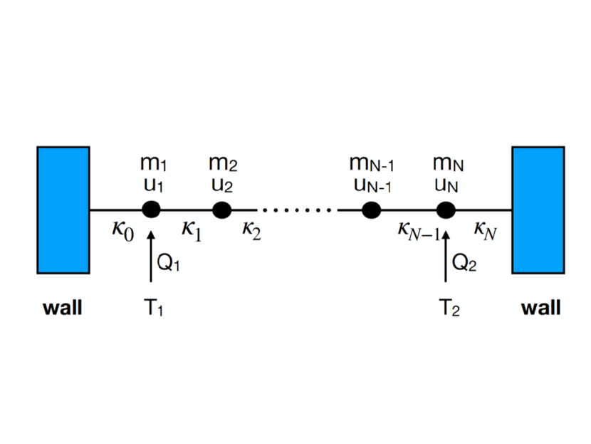
Figure 1: Depiction of the random mass and coupling strength harmonic chain. The particle positions are denoted by $u_{n}$, the masses by $m_{n}$, and the coupling strengths by $\kappa_{n}$. The particles at $n=1$ and $n=N$ are attached to the walls. The chain is driven by heat reservoirs at $n=1$ and $n=N$ transmitting the heat $Q_{1}$ and $Q_{2}$, respectively. The heat reservoirs are maintained at temperatures $T_{1}$ and $T_{2}$, respectively.

where $u_{n}$ is the position of the n-th particle and $\dot{u}_{n}$ its velocity, $\dot{u}_{n}=du_{n}/dt$. We consider fixed boundary conditions, i.e., the chain is attached to walls at the endpoints, yielding the on-site potentials $(1/2)\kappa_{0}u_{1}^{2}$ and $(1/2)\kappa_{N}u_{N}^{2}$. For later purposes we impose both mass disorder and coupling strength disorder, i.e., $m_{n}$ and $\kappa_{n}$ are determined by the independent distributions $\pi_{1}(m_{n})$ and $\pi_{2}(\kappa_{n})$. The chain is driven by two reservoirs at temperatures $T_{1}$ and $T_{2}$, respectively, acting on the first and last particle in the chain. This configuration is depicted in Fig. 1.

The equations of motion in bulk for $1<n<N$ and the Langevin equations for the endpoints for $n=1$ and $n=N$ are given by

$$m_{n}\ddot{u}_{n}(t)=\kappa_{n}u_{n+1}(t)+\kappa_{n-1}u_{n-1}(t)-(\kappa_{n}+\kappa_{n-1})u_{n}(t),~{}~{}1<n<N,$$ (2)

$$m_{1}\ddot{u}_{1}(t)=\kappa_{1}u_{2}(t)-(\kappa_{1}+\kappa_{0})u_{1}(t)-\Gamma\dot{u}_{1}(t)+\xi_{1}(t),$$ (3)

$$m_{N}\ddot{u}_{N}(t)=\kappa_{N-1}u_{N-1}(t)-(\kappa_{N}+\kappa_{N-1})u_{N}(t)-\Gamma\dot{u}_{N}(t)+\xi_{2}(t).$$ (4)

The heat reservoirs at the endpoints are characterised by the white noise correlations

$$\langle\xi_{1}(t)\xi_{1}(t^{\prime})\rangle=2\Gamma T_{1}\delta(t-t^{\prime}),$$ (5)

$$\langle\xi_{2}(t)\xi_{2}(t^{\prime})\rangle=2\Gamma T_{2}\delta(t-t^{\prime});$$ (6)

note that the fluctuation-dissipation theorem Reichl (1998) implies that the damping $\Gamma$ in the Langevin equations is balanced by the damping $\Gamma$ also appearing in the white noise correlations. We, moreover, consider structureless reservoirs characterised by a single damping constant $\Gamma$. The case of memory effects characterised by a frequency dependent damping $\Gamma(\omega)$ has also been discussed, see e.g. Dhar (2001); Casher and Lebowitz (1971). For later purposes we also note that according to (3) and (4) the thermal forces arising from the reservoirs are given by $F_{1}(t)=-\Gamma\dot{u}_{1}(t)+\xi_{1}(t)$ and $F_{2}(t)=-\Gamma\dot{u}_{N}(t)+\xi_{2}(t)$, yielding the heat rates

$$\dot{Q}_{1}(t)=F_{1}(t)\dot{u}_{1}(t),$$ (7)

$$\dot{Q}_{2}(t)=F_{2}(t)\dot{u}_{N}(t).$$ (8)

III Green’s functions

The Green’s function plays an important role in the discussion of heat transport and heat fluctuations. Introducing the Fourier transforms

$$u_{n}(t)=\int\frac{d\omega}{2\pi}\exp(-i\omega t)\tilde{u}_{n}(\omega),$$ (9)

$$\xi_{1,2}(t)=\int\frac{d\omega}{2\pi}\exp(-i\omega t)\tilde{\xi}_{1,2}(\omega),$$ (10)

we can express the equations of motion (2) to (4) in the form

$$\sum_{m=1}^{N}G_{nm}^{-1}(\omega)\tilde{u}_{m}(\omega)=\delta_{n1}{\tilde{\xi}}_{1}(\omega)+\delta_{nN}{\tilde{\xi}}_{2}(\omega),$$ (11)

with solutions

$$\tilde{u}_{n}(\omega)=G_{n1}(\omega)\tilde{\xi}_{1}(\omega)+G_{nN}(\omega)\tilde{\xi}_{2}(\omega),$$ (12)

where the Green’s function $G_{n1}(\omega)$ and $G_{nN}(\omega)$ describe the influence of the coupling to the reservoirs at the endpoints on the particle at site $n$. Here the end-to-end-point Green’s function $G_{1N}(\omega)$ is relevant in the context of heat transfer.

III.0.1 The ordered chain

For the ordered chain with masses $m_{n}=m$ and coupling strengths $\kappa_{n}=\kappa$ the derivation of $G_{1N}(\omega)$ is straightforward in a plane wave basis using an equation of motion approach Fogedby and Imparato (2012) or a determinantal approach Saito and Dhar (2007); Kundu et al. (2011). For a chain composed of $N$ particles one finds the expression

$$G_{1N}(\omega)=\frac{\kappa\sin p}{\kappa^{2}\sin p(N+1)-2i\kappa\Gamma\omega\sin pN-(\Gamma\omega)^{2}\sin p(N-1)},$$ (13)

$$\omega^{2}=\frac{4\kappa}{m}\sin^{2}(p/2),~{}~{}-\pi<p<\pi.$$ (14)

The denominator in (13) shows the resonance structure in the chain. We note that $G_{1N}(\omega)$ is bounded and describes the propagation of ballistic phonons across the chain. The frequency $\omega$ is related to the wavenumber $p$ by the phonon dispersion law (14). The derivation of (13) is presented in Appendix VIII.1.

III.0.2 The disordered chain

The mass-disordered chain has been discussed by Dhar Dhar (2001, 2008), see also Matsuda et al. (1968); Matsuda and Ishii (1970); Ishii (1973). In this context the corresponding end-to-end Greens function $G_{1N}(\omega)$ has been derived. Here we extend this analysis to also include coupling strength disorder. For the disordered chain the plane wave assumption used in obtaining (13) is not applicable owing to the random masses and coupling strengths and one must resort to a transfer matrix method Matsuda and Ishii (1970); Ishii (1973); Dhar (2001).

The transfer matrix $T_{n}(\omega)$ connects the pair of sites $(\tilde{u}_{n}(\omega),\tilde{u}_{n-1}(\omega))$ to the pair of sites $(\tilde{u}_{n+1}(\omega),\tilde{u}_{n}(\omega))$ and thus depends on the local disorder. From the bulk equations of motion (2) in Fourier space we obtain

$$\left(\begin{array}[]{c}\tilde{u}_{n+1}(\omega)\\ \tilde{u}_{n}(\omega)\end{array}\right)=T_{n}(\omega)\left(\begin{array}[]{c}\tilde{u}_{n}(\omega)\\ \tilde{u}_{n-1}(\omega)\end{array}\right),$$ (19)

where the transfer matrix is given by

$$T_{n}(\omega)=\left(\begin{array}[]{cc}\Omega_{n}(\omega)/\kappa_{n}&-\kappa_{n-1}/\kappa_{n}\\ 1&0\end{array}\right);$$ (22)

we have introduced

$$\Omega_{n}(\omega)=\kappa_{n}+\kappa_{n-1}-m_{n}\omega^{2}.$$ (23)

The pair of sites $(\tilde{u}_{N}(\omega),\tilde{u}_{N-1}(\omega))$ are thus related to the pair of sites $(\tilde{u}_{2}(\omega),\tilde{u}_{1}(\omega))$ by a product of random transfer matrices according to

$$\left(\begin{array}[]{c}\tilde{u}_{N}(\omega)\\ \tilde{u}_{N-1}(\omega)\end{array}\right)=T_{N-1}(\omega)T_{N-2}(\omega)\cdots T_{2}(\omega)\left(\begin{array}[]{c}\tilde{u}_{2}(\omega)\\ \tilde{u}_{1}(\omega)\end{array}\right).$$ (28)

Incorporating the coupling to the heat baths at sites $n=1$ and $n=N$ the Green’s function $G_{1N}(\omega)$ takes the form

$$G_{1N}(\omega)=\frac{\kappa_{0}}{\kappa_{0}\kappa_{N}B_{11}(\omega)+i\Gamma\omega(\kappa_{N}B_{12}(\omega)-\kappa_{0}B_{21}(\omega))+(\Gamma\omega)^{2}B_{22}(\omega)}.$$ (29)

Here $B(\omega)$ is given by the matrix product

$$B(\omega)=T_{N}(\omega)T_{N-1}(\omega)\cdots T_{1}(\omega);$$ (30)

note that in the ordered chain, $m_{n}=m$ and $\kappa_{n}=\kappa$, and we have $T_{n}(\omega)=T(\omega)$, i.e., $B(\omega)=T^{N}(\omega)$. By insertion of $T^{N}(\omega)$ given by (153) we readily obtain (13). The derivation of (29) is given in Appendix VIII.1.

IV The Liapunov exponent

The Liapunov exponent is of importance in determining the properties of the disordered chain. For large $N$ the behaviour of $G_{1N}(\omega)$ in (29) is determined by the asymptotic properties of the matrix product $B(\omega)$ in (30) . This issue has been discussed extensively in seminal papers by Matsuda and Ishii Matsuda et al. (1968); Matsuda and Ishii (1970); Ishii (1973) on the basis of the Furstenberg theorem Furstenberg (1963); O’Connor (1975). A central result is that

$$\lim_{N\rightarrow\infty}\frac{1}{N}\log(|\tilde{u}_{N}(\omega)|^{2}+|\tilde{u}_{N-1}(\omega)|^{2})=2\gamma(\omega)$$ (31)

with probability one; this is basically an expression of the law of large numbers applied to non commuting independent random matrices. Here $\gamma(\omega)$ is a positive Liapunov exponent depending on the phonon frequency $\omega$ and the disorder. For the norm we infer the scaling behaviour

$$|\tilde{u}_{N}(\omega)|\propto\exp(\gamma(\omega)N),$$ (32)

and since the matrix $T_{N}^{-1}(\omega)B(\omega)T_{1}^{-1}(\omega)$ according to (28) connects the pair of site $(\tilde{u}_{N}(\omega),\tilde{u}_{N-1}(\omega))$ to the pair of sites $(\tilde{u}_{2}(\omega),\tilde{u}_{1}(\omega))$, the matrix elements $B_{nm}(\omega)$, likewise, scale like

$$|B_{nm}(\omega)|\propto\exp(\gamma(\omega)N)$$ (33)

for large $N$. For vanishing disorder $\gamma(\omega)=0$ and $B(\omega)$ is bounded, i.e., not growing with $N$. It then follows from (29) that $G_{1N}(\omega)$, likewise, is bounded.

Introducing the ratio $z_{n}(\omega)=\tilde{u}_{n}(\omega)/\tilde{u}_{n-1}(\omega)$ and inserting (23), it follows from the bulk equations of motion (2) that $z_{n}(\omega)$ obeys the non linear stochastic discrete map

$$z_{n+1}(\omega)=\frac{\kappa_{n}+\kappa_{n-1}-m_{n}\omega^{2}}{\kappa_{n}}-\frac{\kappa_{n-1}}{\kappa_{n}}\frac{1}{z_{n}(\omega)}.$$ (34)

We also note from (32) that for large $N$ we have $|z_{N}(\omega)|=|\tilde{u}_{N}(\omega)|/|\tilde{u}_{N-1}(\omega)|\propto\exp(\gamma(\omega))$ or

$$\gamma(\omega)=\lim_{N\rightarrow\infty}\log|z_{N}(\omega)|.$$ (35)

Consequently, the Liapunov exponent $\gamma(\omega)$ is determined by the asymptotic properties of the map (34) for large $N$.

More precisely, in general the map (34) is stochastic due to the randomness of $m_{n}$ and $\kappa_{n}$. However, just as a white Gaussian noise $\xi(t)$ with correlations $\langle\xi(t)\xi(t^{\prime})\rangle=2\Delta\delta(t-t^{\prime})$ in a Langevin equation of the form $dx(t)/dt=-dV(x)/dx+\xi(t)$ for a stochastic variable $x(t)$ can drive $x$ into a stationary distribution $P_{0}(x)\propto\exp(-V/\Delta)$ Reichl (1998), we anticipate that the ’noise’ due to the randomness of $m$ and $\kappa$ will drive $z_{n}$ into a stationary distribution $P_{0}(z)$. Consequently, according to (35) we infer

$$\gamma(\omega)=\int dzP_{0}(z)\log|z(\omega)|.$$ (36)

The task is thus to determine $P_{0}(z)$ on the basis of the map (34) and evaluate $\gamma(\omega)$.

V Coupling strength disorder

For general values of the frequency the Liapunov exponent $\gamma(\omega)$ is not available in explicit analytical form. However, Matsuda et al. Matsuda et al. (1968); Matsuda and Ishii (1970) have determined $\gamma(\omega)$ in the low frequency limit in the case of mass disorder. They find

$$\gamma(\omega)\simeq\frac{1}{8}\frac{\omega^{2}}{\kappa\langle m\rangle}\langle\delta m^{2}\rangle,$$ (37)

where the mean mass and the mean square mass deviations are given by $\langle m\rangle$ and $\langle\delta m^{2}\rangle=\langle(m-\langle m\rangle)^{2}\rangle$; the averages $\langle\cdots\rangle$ determined by the mass distribution $\pi_{1}(m_{n})$.

Here we consider the evaluation of the Liapunov exponent in the case of coupling strength disorder. Rather than attempting to apply the techniques by Matsuda et al. we here use an approach advanced by Lepri et al. Lepri et al. (2003) using dynamical system theory Jackson (1990) and statistical physics Reichl (1998). From a theoretical physics point a view we believe this method is simpler and more straightforward.

V.1 The case: $\omega=0$, $m_{n}=m$, $\kappa_{n}=\kappa$

For $\omega=0$ and vanishing disorder, i.e., $\kappa_{n}=\kappa$ and $m_{n}=m$ the map (34) takes the form

$$z_{n+1}=f(z_{n})=2-\frac{1}{z_{n}},$$ (38)

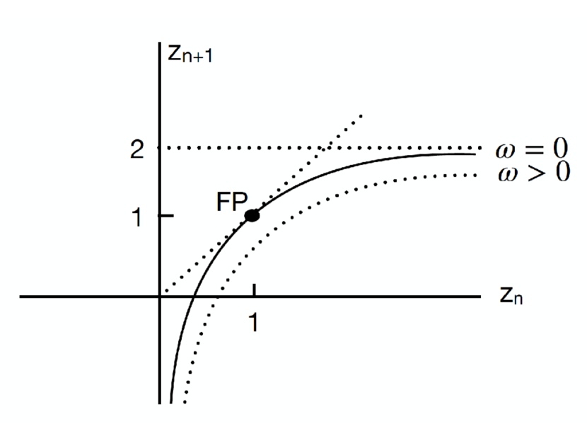
Figure 2: Depiction of the phase diagram of the discrete nonlinear map in a plot of $z_{n+1}$ versus $z_{n}$. The map has a marginally stable fixed point (FP) at $z\ast=1$. The full curve for $\omega=0$ corresponds to the map (38); the dotted curve for $\omega>0$ corresponds to the map (39).

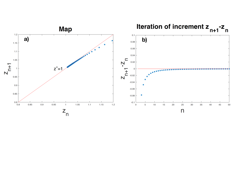
Figure 3: In a) we plot $z_{n+1}$ versus $z_{n}$ and depict the iteration of the map for $\omega=0$ in (38). The iterates converge towards the marginally stable fixed point (FP) at $z\ast=1$. In b) we depict the increments as function of $n$, showing the convergence to the fixed point.

where we have omitted the $\omega$ dependence. In a plot of $z_{n+1}$ versus $z_{n}$ the map is composed of two hyperbolic branches. For $|z_{n}|\rightarrow\infty$ we have $z_{n+1}\rightarrow 2$, for $z_{n}\rightarrow\pm 0$ we note that $z_{n+1}\rightarrow\mp\infty$. The map has a fixed point $z^{\ast}$ determined by $f(z^{\ast})=z^{\ast}$, yielding $z^{\ast}=1$. The evolution of the iterates as a function of $n$ is analysed by considering the increment $z_{n+1}-z_{n}=-(z_{n}-1)^{2}/z_{n}$. We find that $z_{n+1}-z_{n}<0$ for $z_{n}>0$, whereas for $z_{n}<0$ the increment $z_{n+1}-z_{n}>0$. At the fixed point $z^{\ast}=1$ the increment vanishes, i.e, $z_{n+1}-z_{n}=0$. In other words, as we approach the fixed point through iterates $z_{n}>1$ the iterates converge to the fixed point; on the other hand, choosing an initial iterate $z_{n}\lesssim 1$ the iterates move away from the fixed point, corresponding to a marginally stable fixed point. Further inspection of the map in a plot of $z_{n+1}$ versus $z_{n}$ shows that choosing an initial value $z_{n}<1$ the iterates eventually make a single excursion to the hyperbola $2-1/z_{n}$ for $z_{n}<0$ before returning to the hyperbola for $z_{n}>0$ and approaching the fixed point. In Fig. 2 we have plotted $z_{n+1}$ versus $z_{n}$ with the fixed point indicated at $z_{n+1}=z_{n}=1$; the solid line depicts the map (38). In Fig. 3 we have in a) plotted $z_{n+1}$ versus $z_{n}$ demonstrating the convergence towards the fixed point at $z^{\ast}=1$; in b) we have plotted the decreasing increments $z_{n+1}-z_{n}$ versus $n$.

V.2 The case: $\omega\gtrsim 0$, $m_{n}=m$, $\kappa_{n}=\kappa$

We next consider the case of small $\omega$ and vanishing disorder. From (34) we infer the map

$$z_{n+1}=2-\frac{m}{\kappa}\omega^{2}-\frac{1}{z_{n}},$$ (39)

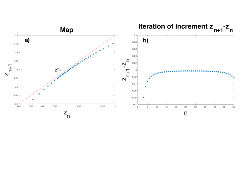
Figure 4: In a) we plot $z_{n+1}$ versus $z_{n}$ and depict the iteration of the map for $\omega>0$ in (39). The iterates compress and flow past the point $z=1$ (the position of fixed point (FP) $z\ast=1$ for $\omega=0$). In b) we depict the increments as function of $n$, showing the compression near the the point $z=1$, allowing for a continuum approximation.

depicted by a dotted line in Fig. 2. In this case the map does not have a (real) fixed point. However, analysing the increment $z_{n+1}-z_{n}=2-(m/\kappa)\omega^{2}-z_{n}-1/z_{n}$ in the vicinity of the value $z=1$ (the position of the fixed point for $\omega=0$) we obtain $z_{n+1}-z_{n}\approx-(m/\kappa)\omega^{2}$ and the increment vanishes for small $\omega$. We note that the increment is negative corresponding to a flux of iterates close to the point $z=1$ from the region $z_{n}>1$ to $z_{n}<1$. In Fig. 4 we have in a) plotted $z_{n+1}$ versus $z_{n}$ demonstrating the flux of iterates past the point $z=1$; in b) we have shown that the increments $z_{n+1}-z_{n}$ as function of $n$ decrease in the vicinity of the point $z=1$.

V.3 The case: $\omega\gtrsim 0$, $m_{n}=m$, $\delta\kappa_{n}\approx 0$

Finally, we consider the case of small $\omega$ and small coupling strength disorder. Setting $\kappa_{n}=\langle\kappa\rangle+\delta\kappa_{n}$, where $\langle\kappa\rangle$ is determined by the coupling strength distribution $\pi_{2}(\kappa_{n})$, and assuming $\delta\kappa_{n}\ll\langle\kappa\rangle$, we obtain to leading order expanding the map (34)

$$z_{n+1}=2-\frac{m}{\langle\kappa\rangle}\bigg{(}1-\frac{\delta\kappa_{n}}{\langle\kappa\rangle}\bigg{)}\omega^{2}+\frac{\delta\kappa_{n-1}-\delta\kappa_{n}}{\langle\kappa\rangle}-\bigg{(}1+\frac{\delta\kappa_{n-1}-\delta\kappa_{n}}{\langle\kappa\rangle}\bigg{)}\frac{1}{z_{n}}.$$ (40)

Furthermore, expanding about the point $z=1$ by setting $z_{n}=1+\epsilon_{n}$ we note that the terms $(\delta\kappa_{n-1}-\delta\kappa_{n})/\langle\kappa\rangle$ cancels out and we obtain for small $\epsilon_{n}$

$$\epsilon_{n+1}-\epsilon_{n}\simeq-\epsilon_{n}^{2}-\frac{m}{\langle\kappa\rangle}\omega^{2}+\frac{m\omega^{2}}{\langle\kappa\rangle^{2}}\delta\kappa_{n}.$$ (41)

For large $n$ the iterates compress and constitute a flow near the point $z=1$ in the sense that $\epsilon_{n}-\epsilon_{n+1}\rightarrow 0$ for small $\omega$. As a consequence we can introduce the continuum limit and make the assumption $\epsilon_{n}\approx\epsilon(n)$ and $\delta\kappa_{n}\approx\delta\kappa(n)$, where $n$ is a continuous variable. From (41) we thus obtain the effective Langevin equation

$$\frac{d\epsilon(n)}{dn} = -\epsilon(n)^{2}-\frac{m}{\langle\kappa\rangle}\omega^{2}+\eta(n),$$ (42)

$$\eta(n) = \frac{m\omega^{2}}{\langle\kappa\rangle^{2}}\delta\kappa(n),$$ (43)

where we have introduced the ’noise variable’ $\eta(n)$ with correlations

$$\langle\eta(n)\eta(n^{\prime})\rangle=\Delta\delta(n-n^{\prime}),$$ (44)

$$\Delta=\bigg{(}\frac{m\omega^{2}}{\langle\kappa\rangle^{2}}\bigg{)}^{2}\langle\delta\kappa^{2}\rangle.$$ (45)

Expressing the Langevin equation in (42) in the form $d\epsilon/dn=-dV/d\epsilon+\eta$ the ’potential’ has the form $V=(m/\langle\kappa\rangle)\omega^{2}\epsilon+\epsilon^{3}/3$ with a linear slope for small $\epsilon$. Since there is no minimum the ’position’ $\epsilon$ ’falls down’ the slope and escapes for negative $\epsilon$. This is consistent with the behaviour of the iterates near the the point $z=1$ where there is a flow from right to left implying that the stochastic map generates a probability current $J_{0}$ near $z=1$.

In order to proceed we assume that the coupling strength distribution $\pi_{2}(\kappa)$ has a Gaussian form, implying that the ’noise’ driving the Langevin equation (42) has the structure of Gaussian white noise Reichl (1998). This implies that the probability density $P(\epsilon,n)$ is governed by the Fokker-Planck equation Risken (1989)

$$\frac{\partial P(\epsilon,n)}{\partial n}=\frac{\partial}{\partial\epsilon}\Big{(}\epsilon^{2}+\frac{m}{\langle\kappa\rangle}\omega^{2}\Big{)}P(\epsilon,n)+\frac{1}{2}\Delta\frac{\partial^{2}P(\epsilon,n)}{\partial\epsilon^{2}}.$$ (46)

From the continuity equation $\partial P/\partial n=-\partial J_{0}/\partial\epsilon$ we identify the probability current

$$J_{0}=-\Big{(}\epsilon^{2}+\frac{m}{\langle\kappa\rangle}\omega^{2}\Big{)}P(\epsilon,n)-\frac{1}{2}\Delta\frac{\partial P(\epsilon,n)}{\partial\epsilon}.$$ (47)

For small $\omega$ the stationary distribution to leading asymptotic order in $\Delta$ has the form

$$P_{0}(\epsilon)\propto\frac{1}{\epsilon^{2}+(m/\langle\kappa\rangle)\omega^{2}}+\Delta\frac{\epsilon}{(\epsilon^{2}+(m/\langle\kappa\rangle)\omega^{2})^{3}},$$ (48)

for a technical detail see Appendix VIII.2. Finally, from (35), expanding $\log(|z(\omega)|)\sim 1+\epsilon(\omega)$, we have

$$\gamma(\omega)=\frac{\int d\epsilon\epsilon P_{0}(\epsilon)}{\int d\epsilon P_{0}(\epsilon)}.$$ (49)

Inserting $P_{0}(\epsilon)$ we note that the first term in (48) for symmetry reasons does not contribute and we obtain by quadrature to order $\Delta$ the Liapunov exponent for small $\omega$ for a coupling strength-disordered chain

$$\gamma(\omega)\simeq\frac{1}{8}\frac{\omega^{2}}{\langle\kappa\rangle m}\bigg{(}\frac{m}{\langle\kappa\rangle}\bigg{)}^{2}\langle\delta\kappa^{2}\rangle.$$ (50)

V.4 Combining coupling strength disorder and mass disorder

Here we consider as a corollary the case of both coupling strength disorder and mass disorder. In the map (34) we note that in the absence of coupling strength disorder the random mass $m_{n}$ multiplies $\omega$ and is quenched in the low frequency limit. In the analysis by Matsuda et al. Matsuda et al. (1968); Matsuda and Ishii (1970) the Liapunov exponent in (37) only depends on the first and second moment of the mass distribution, i.e., $\langle m\rangle$ and $\langle\delta m^{2}\rangle$. In other words, the calculation of (37) does not presuppose a narrow mass distribution.

Including mass disorder in the Langevin equation in (42) by setting $m(n)=\langle m\rangle+\delta m(n)$ we obtain

$$\frac{d\epsilon(n)}{dn} = -\epsilon(n)^{2}-\frac{\langle m\rangle}{\langle\kappa\rangle}\omega^{2}+\tilde{\eta}(n),$$ (51)

$$\tilde{\eta}(n) = \frac{\langle m\rangle\omega^{2}}{\langle\kappa\rangle^{2}}\delta\kappa(n)-\frac{\omega^{2}}{\langle\kappa\rangle}\delta m(n).$$ (52)

Ignoring terms of order $\delta m\delta\kappa$ we obtain the noise correlations

$$\langle\tilde{\eta}(n)\tilde{\eta}(n^{\prime})\rangle=\tilde{\Delta}\delta(n-n^{\prime}),$$ (53)

$$\tilde{\Delta}=\bigg{(}\frac{\omega^{2}}{\langle\kappa\rangle}\bigg{)}^{2}\bigg{[}\langle\delta m^{2}\rangle+\bigg{(}\frac{\langle m\rangle}{\langle\kappa\rangle}\bigg{)}^{2}\langle\delta\kappa^{2}\rangle\bigg{]},$$ (54)

and correspondingly the Liapunov exponent

$$\tilde{\gamma}(\omega)\simeq\frac{1}{8}\frac{\omega^{2}}{\langle\kappa\rangle\langle m\rangle}\langle\delta\tilde{m}^{2}\rangle,$$ (55)

$$\langle\delta\tilde{m}^{2}\rangle=\langle\delta m^{2}\rangle+\bigg{(}\frac{\langle m\rangle}{\langle\kappa\rangle}\bigg{)}^{2}\langle\delta\kappa^{2}\rangle.$$ (56)

For $\delta\kappa=0$ we recover the Liapunov exponent in the mass-disordered case in (37) first derived by Matsuda et al. Matsuda et al. (1968); Matsuda and Ishii (1970), see also Lepri et al. (2003). The presence of weak coupling strength disorder can be incororated by introducing the renormalised mean square mass deviation $\langle\delta\tilde{m}^{2}\rangle$ given by (56). The expressions in (50) and (55-56) constitute the main results of the present analysis.

V.5 Connection to 1D quantum mechanical disorder

The Langevin equations in (42) and (51) have the form of a Ricatti equation of the form $\epsilon^{\prime}=-\epsilon^{2}-E+V$, where $V=\tilde{\eta}$ and $E=\omega^{2}\langle m\rangle/\langle\kappa\rangle$, the prime denoting a derivative. By means of the substitution $\epsilon=\psi^{\prime}/\psi$ the Ricatti equation is reduced to the 1D stationary Schrödinger equation, $-\psi^{\prime\prime}+V\psi=E\psi$, describing the quantum motion in a random potential $V$ with zero mean and ”white noise”correlations $\langle\tilde{\eta}(n)\tilde{\eta}(n^{\prime})\rangle=\tilde{\Delta}\delta(n-n^{\prime})$. This problem, relating to Anderson localisation Anderson (1958), has been studied extensively, see e.g. Nieuwenhuizen (1983); Lifshits et al. (1988); Luck (2004); Grabsch et al. (2014). In 1D in the presence of even weak disorder the wave function is localised, characterised by the localisation or correlation length $l_{c}$. The corresponding Liapunov exponent is thus given by $\gamma=1/l_{c}$. According to the analysis by Luck Luck (2004) one finds in the case of weak disorder $\gamma=\tilde{\Delta}/8E$ and by insertion the result in (55).

VI Heat Current and heat fluctuations

Here we briefly discuss the implication of a Liapunov exponent for the heat current and heat fluctuations.

VI.1 Heat Current

Regarding the heat current we summarise the analysis by Dhar Dhar (2001, 2008); Dhar and Saitou (2016) below. According to (7) the fluctuating heat rate from reservoir 1 is given by $\dot{Q}(t)=(-\Gamma\dot{u}_{1}(t)+\xi_{1}(t))\dot{u}_{1}(t)$ and the integrated heat flux by $Q(t)=\int^{t}dt^{\prime}\dot{Q}(t^{\prime})$. Averaged over the heat reservoirs the mean value $\langle Q(t)\rangle\propto t$ and we obtain the mean heat current $J(N)=\langle Q(t)\rangle/t$, $\langle\cdots\rangle$ denoting a thermal average.

For an ordered chain the mean heat current is given by the expression Casher and Lebowitz (1971); Rubin and Greer (1971); Dhar and Roy (2006); Dhar (2008); Fogedby and Imparato (2012)

$$J(N)=\frac{1}{2}(T_{1}-T_{2})\int\frac{d\omega}{2\pi}T(\omega),$$ (57)

where the transmission matrix $T(\omega)$ is expressed in terms of the end-to-end Green’s function in (13),

$$T(\omega)=4(\omega\Gamma)^{2}|G_{1N}(\omega)|^{2}.$$ (58)

Since $T(\omega)$ is bounded and the range of $\omega$ is determined by the phonon dispersion law (14) it follows that the heat current $J\propto(T_{1}-T_{2})$, yielding a conductivity $\kappa\propto N$; this behaviour is characteristic of ballistic heat transport.

In Appendix VIII.3 we have derived the expression (57), see also Fogedby and Imparato (2012), and find that it also holds for the disordered chain with the Green’s function (29) for a particular disorder realisation $\{m_{n}\}$ and $\{\kappa_{n}\}$. The issue of averaging the current $J(N)$ with respect to the disorder is, however, quite complex and we review the analysis by Dhar Dhar (2001, 2008); Dhar and Saitou (2016) here.

For a system of size $N$ the matrix elements $B_{ij}(\omega)$ in $G_{1N}(\omega)$ scale according to (33) like $\exp(\tilde{\gamma}(\omega)N)$, where $\tilde{\gamma}(\omega)$ for small $\omega$ and both mass disorder and weak coupling strength disorder is given by (55) and (56) . Consequently, for $\tilde{\gamma}(\omega)N\gg 1$ the denominator in $G_{1N}(\omega)$ diverges and the heat current vanishes; this is due to the localised modes which do not carry energy and thus do not contribute to the heat transport. On the other hand, for $\tilde{\gamma}(\omega)N\ll 1$, corresponding to the extended modes, the Green’s function $G_{1N}(\omega)$ is bounded and contributes to the heat current.

The limiting case for $\tilde{\gamma}(\omega)N\approx 1$ defines the correlation or cross-over frequency

$$\omega_{c}=(8\langle\kappa\rangle\langle m\rangle)^{1/2}(\langle\delta\tilde{m}^{2}\rangle N)^{-1/2}.$$ (59)

Consequently, the integration over frequencies in (57) is cut-off at $\omega=\omega_{c}$. An approximate expression for the disorder-averaged heat current, characterised by a bar, is thus given by

$$\overline{J(N)}\simeq\frac{1}{2}(T_{1}-T_{2})\int_{-\omega_{c}}^{\omega_{c}}\frac{d\omega}{2\pi}T(\omega).$$ (60)

Owing to the $N$-dependence of the cut-off frequency $\omega_{c}$ the heat current $\overline{J(N)}$ acquires an explicit $N$ dependence. In the range $|\omega|<\omega_{c}$ of extended modes Dhar Dhar (2001, 2008) uses for $G_{1N}(\omega)$ the unperturbed result given by (13). This is an excellent approximation supported by numerical estimates Dhar (2008). Since $T(\omega)\sim\omega^{2}$ for small $\omega$ a simple scaling argument yields $\overline{J(N)}\sim\omega_{c}^{3}\sim(\langle\delta\tilde{m}^{2}\rangle N)^{-3/2}$, corresponding to the exponent $\alpha=3/2$; note that in the ballistic case $\alpha=0$. We also find that the heat current for large fixed $N$ scales with the mean square renormalised mass according to $\overline{J(N)}\sim\langle\delta\tilde{m}^{2}\rangle^{-3/2}$.

VI.2 Large deviation function

The distribution of heat fluctuations is described by the moment generating characteristic function Reichl (1998)

$$C(\lambda,t)=\langle\exp(\lambda Q(t))\rangle.$$ (61)

Correspondingly, the cumulant generating function is given by $\log C(\lambda,t)$. The long time behaviour is characterised by the associated large deviation function $\mu(\lambda)$ according to

$$C(\lambda,t)=\exp(\mu(\lambda)t).$$ (62)

It follows from general principles Touchette (2009); den Hollander (2000); Fogedby and Imparato (2011, 2012, 2014) that the cumulant generating function $\mu(\lambda)$ is downward convex and owing to normalisation passes through the origin, i.e., $\mu(0)=0$.

For an ordered chain the large deviation function has been derived by Saito and Dhar Saito and Dhar (2007, 2011), see also Kundu et al. (2011). Here we present a derivation in Appendix VIII.4, see also Fogedby and Imparato (2012). The large deviation function has the form

$$\mu(\lambda)=-\frac{1}{2}\int\frac{d\omega}{2\pi}\log[1+T(\omega)f(\lambda)],$$ (63)

$$T(\omega)=4(\omega\Gamma)^{2}|G_{1N}(\omega)|^{2},$$ (64)

$$f(\lambda)=T_{1}T_{2}\lambda(1/T_{1}-1/T_{2}-\lambda).$$ (65)

Here the structure of $f(\lambda)$ ensures that $\mu(\lambda)$ satisfies the Gallavotti-Cohen fluctuation theorem Gallavotti and Cohen (1995); Lebowitz and Spohn (1999); Fogedby and Imparato (2012) valid for driven non equilibrium systems,

$$\mu(\lambda)=\mu(1/T_{1}-1/T_{2}-\lambda).$$ (66)

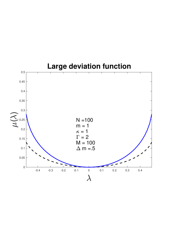
Figure 6: We depict the large deviation function $\mu(\lambda)$ as a function of $\lambda$ for $N=100$, $m=1$, $\kappa=1$, and $\Gamma=2$. The blue curve refers to the ordered chain, i.e., in the absence of disorder. The black dashed curve refers to the disordered case for $\Delta m=0.5$ averaged over $M=100$ samples. Since $T(\omega)$ is reduced in the upper $\omega$ range the large deviation function sampling all frequencies is overall reduced. However, since $f(\lambda)$ has the form of an inverted parabola, the reduction of $\overline{\mu(\lambda)}$ is most pronounced for $\lambda$ close to the edges.

From the structure of (63) it follows that $\mu(\lambda)$ has branch points determined by the condition $1+T(\omega)f(\lambda)>0$. Since by inspection $0\leq T(\omega)\leq 1$, see Fogedby and Imparato (2012), it follows that $f(\lambda)>-1$ yielding the branch points $\lambda_{1}=1/T_{1}$ and $\lambda_{2}=-1/T_{2}$. We also note that the fluctuation theorem in (66) implies that $\mu(1/T_{1}-1/T_{2})=0$. In conclusion, the large deviation function is downward convex, crossing the axis at $\lambda=0$ and $\lambda=1/T_{1}-1/T_{2}$ and having branch points at $\lambda_{1}$ and $\lambda_{2}$. At equal temperature $T_{1}=T_{2}$ the large deviation function is positive in the whole range as shown in Fig. 6.

The expression for $\mu(\lambda)$ in (63) is for a concrete realisation of the quenched mass and coupling strength disorder $\{m_{n}\}$ and $\{\kappa_{n}\}$ through the dependence on the Green’s function $G_{1N}(\omega)$ in (29). We note, however, that due to the form of $f(\lambda)$ the large deviation function $\mu(\lambda)$ satisfies the Gallavotti-Cohen fluctuation theorem for each disorder realisation and we conclude that the disorder-averaged large deviation function $\overline{\mu(\lambda)}$, likewise, obeys the fluctuation theorem.

A further clarification also follows from the Fokker-Planck equation for the joint distribution $P(Q_{1},Q_{2},\{u_{n}\},\{\dot{u}_{n}\},t)$ for the heat transfer Imparato et al. (2007); Fogedby and Imparato (2012); Risken (1989)

$$\frac{\partial P}{\partial t}= (L_{0}+L_{Q})P,$$ (67)

$$L_{0}P= \{P,H\},$$ (68)

$$L_{Q}P= \Gamma\Bigg{(}T_{1}\dot{u}_{1}^{2}\frac{\partial^{2}P}{\partial Q_{1}^{2}}+2T_{1}\dot{u}_{1}\frac{\partial^{2}P}{\partial Q_{1}\partial\dot{u}_{1}}+(\dot{u}_{1}^{2}+T_{1})\frac{\partial P}{\partial Q_{1}}\Bigg{)}$$

$$+ \Gamma\Bigg{(}T_{2}\dot{u}_{N}^{2}\frac{\partial^{2}P}{\partial Q_{2}^{2}}+2T_{2}\dot{u}_{N}\frac{\partial^{2}P}{\partial Q_{2}\partial\dot{u}_{N}}+(\dot{u}_{N}^{2}+T_{2})\frac{\partial P}{\partial Q_{2}}\Bigg{)}.$$ (69)

As shown in Fogedby and Imparato (2012) the fluctuation theorem here follows from the structure of the operator $L_{Q}$ and does not depend on the Hamiltonian part $L_{0}P$. Since the disorder only enters in the Hamiltonian $H$ in (1) we again infer the validity of the fluctuation theorem.

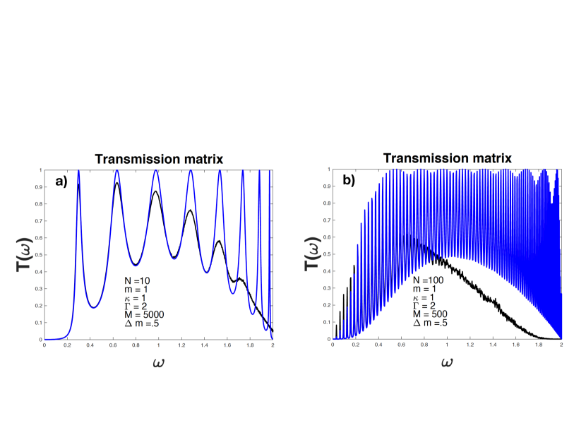
Figure 5: In a) we depict the transmission matrix $T(\omega)$ as a function of $\omega$ for $N=10$, $m=1$, $\kappa=1$, and $\Gamma=2$. The blue curve refers to the ordered chain, i.e., in the absence of disorder, showing the resonance structure in $G_{1N}(\omega)$. The black curve refers to the disordered case for $\Delta m=0.5$ averaged over $M=5000$ samples. In b) we depict $T(\omega)$ for $N=100$ and $M=500$. In both cases black curve displays the reduction of $T(\omega)$ for larger frequencies due to the disorder.

The disorder enters in the transmission matrix $T(\omega)$ given by (58). In Fig. 5 we have in a) depicted the transmission matrix for $N=10$, $m=1$, $\kappa=1$, and $\Gamma=2$. The blue curve refers to the ordered case for $\langle\delta\tilde{m}^{2}\rangle=0$, showing the resonance structure of $G_{1N}(\omega)$. The black curve corresponds to the disordered case for $\sqrt{\langle\delta\tilde{m}^{2}\rangle}=0.5$ averaged over 5000 samples. With this choice of parameters the cross-over frequency in (59) is $\omega_{c}\sim 1.8$ in accordance with Fig. 5, showing the onset of localised states for $\omega>\omega_{c}$, yielding a decreasing transmission matrix; in Fig. 5 we have in b) depicted $T(\omega)$ for $N=100$ and $500$ samples showing the same features.

Finally, implementing the same approximation as for the heat current in (60), we express the disorder-averaged large deviation function in the form

$$\overline{\mu(\lambda)}\simeq-\frac{1}{2}\int_{-\omega_{c}}^{\omega_{c}}\frac{d\omega}{2\pi}\log[1+T(\omega)f(\lambda)],$$ (70)

where $T(\omega)=4(\omega\Gamma)^{2}|G_{1N}(\omega)|^{2}$ is expressed in terms of the Green’s function $G_{1N}(\omega)$ for the ordered case in (13). We have not investigated the expression in (70) further but have determined $\overline{\mu(\lambda)}$ numerically. In Fig. 6 we have depicted the large deviation function for $N=100$ both in the absence of disorder for $\delta\tilde{m}=0$ and in the presence of disorder choosing $\delta\tilde{m}=0.5$. Since $T(\omega)$ is reduced in the upper $\omega$ range the large deviation function sampling all frequencies is overall reduced. However, since $f(\lambda)$ has the form of an inverted parabola, the reduction of $\overline{\mu(\lambda)}$ is most pronounced for $\lambda$ close to the edges, as shown in Fig. 6.

VII Conclusion

In this paper we have discussed the disordered harmonic chain subject to coupling strength disorder. A case which to our knowledge has not been studied previously. Using a dynamical system theory approach we have evaluated the Liapunov exponent at low frequency and for weak coupling strength disorder. Including mass disorder we have obtained an expression for the Liapunov exponent which interpolates between coupling strength disorder and mass disorder. In the absence of coupling strength disorder we recover the well-known result by Matsuda et al., see also Lepri. In the general case coupling strength disorder can be incorporated by introducing a renormalised mass disorder. Finally, we have discussed the heat current and the large deviation function and commented on the validity of the Gallavotti-Cohen fluctuation theorem for the disordered chain.

VIII Appendix

VIII.1 Greens function

Inserting (23) we have in Fourier space the Langevin equations

$$\Omega_{1}(\omega)\tilde{u}_{1}(\omega)=i\omega\Gamma\tilde{u}_{1}(\omega)+\kappa_{1}\tilde{u}_{2}(\omega)+\tilde{\xi}_{1}(\omega),$$ (71)

$$\Omega_{N}(\omega)\tilde{u}_{N}(\omega)=i\omega\Gamma\tilde{u}_{N}(\omega)+\kappa_{N-1}\tilde{u}_{N-1}(\omega)+\tilde{\xi}_{2}(\omega),$$ (72)

and we infer that the inverse Green’s function in (11) has the form

$$G^{-1}(\omega)=\left(\begin{array}[]{ccccc}\tilde{\Omega}_{1}(\omega)&-\kappa_{1}&&&\\ -\kappa_{1}&\Omega_{2}(\omega)&-\kappa_{2}&&\\ &-\kappa_{2}&\cdots&&\\ &&&\Omega_{N-1}(\omega)&-\kappa_{N-1}\\ &&&-\kappa_{N-1}&\tilde{\Omega}_{N}(\omega)\end{array}\right),$$ (78)

where $\tilde{\Omega}_{1}(\omega)=\Omega_{1}(\omega)-i\Gamma\omega$ and $\tilde{\Omega}_{N}(\omega)=\Omega_{N}(\omega)-i\Gamma\omega$. We note that $G^{-1}(\omega)$ is a symmetric tridiagonal matrix. For the matrix elements we thus have $G_{nm}^{-1}(\omega)=G_{mn}^{-1}(\omega)$ implying $G_{nm}(\omega)=G_{mn}(\omega)$. The symmetry and structure also allows us to derive the useful Schwinger identity Wang and Uhlenbeck (1945). From (78) we have, the $\ast$ indicting a complex conjugate,

$$G_{nm}^{-1}(\omega)-G_{nm}^{-1\ast}(\omega)=((\tilde{\Omega}_{1}(\omega)-\tilde{\Omega}_{1}^{\ast}(\omega))\delta_{n1}+(\tilde{\Omega}_{N}(\omega)-\tilde{\Omega}_{N}^{\ast}(\omega))\delta_{nN})\delta_{nm},$$ (79)

or

$$G_{nm}^{-1}(\omega)-G_{nm}^{-1\ast}(\omega)=-2i\omega\Gamma(\delta_{n1}+\delta_{nN})\delta_{nm}.$$ (80)

Multiplying by $G(\omega)$ on the left and $G^{\ast}(\omega)$ on the right and using the symmetry of $G_{nm}(\omega)$ we obtain the Schwinger identity Wang and Uhlenbeck (1945)

$$G_{nm}(\omega)-G_{nm}^{\ast}(\omega)=2i\omega\Gamma(G_{n1}(\omega)G_{1m}^{\ast}(\omega)+G_{nN}(\omega)G_{Nm}^{\ast}(\omega));$$ (81)

the Schwinger identity in (81) is used later in Appendices VIII.3 and VIII.4 in deriving the heat current and the cumulant generating function.

VIII.1.1 Ordered chain - equation of motion method

In the ordered case for $m_{n}=m$ and $\kappa_{n}=\kappa$ the Green’s functions $G_{n1}(\omega)$ and $G_{nN}(\omega)$ are easily determined by an equation of motion method. Alternatively, one can employ a determinantal scheme noting that the determinant of $G^{-1}(\omega)$ for $\tilde{\Omega}_{1}=\tilde{\Omega}_{N}=\Omega$ is given by $\kappa^{N}U_{N}(\Omega/2\kappa)$, where $U_{N}(x)$ is the Chebychev polynomial of the second kind; $U_{N}(\Omega/2\kappa)=\sin p(N+1)/\sin p,\Omega=2\kappa\cos p$ Lebedev (1972).

Addressing the equations of motion, which are of the linear difference form,

$$\Omega\tilde{u}_{n}(\omega)=\kappa(\tilde{u}_{n+1}(\omega)+\tilde{u}_{n-1}(\omega)),$$ (82)

$$\Omega\tilde{u}_{1}(\omega)=i\Gamma\omega\tilde{u}_{1}(\omega)+\kappa\tilde{u}_{2}(\omega)+\tilde{\xi}_{1}(\omega),$$ (83)

$$\Omega\tilde{u}_{N}(\omega)=i\Gamma\omega\tilde{u}_{N}(\omega)+\kappa\tilde{u}_{N-1}(\omega)+\tilde{\xi}_{2}(\omega),$$ (84)

and using the plane wave ansatz $\tilde{u}_{n}=A\exp(ipn)+B\exp(-ipn)$ equation (82) yields $\Omega=2\kappa\cos p=\kappa(\exp(ip)+\exp(-ip))$. Inserting $\Omega$ in (83) and (84) we obtain for the determination of $A$ and $B$ the matrix equation

$$\left(\begin{array}[]{cc}\kappa-i\Gamma\omega e^{ip}&\kappa-i\Gamma\omega e^{-ip}\\ (\kappa e^{ip}-i\Gamma\omega)e^{ipN}&(\kappa e^{-ip}-i\Gamma\omega)e^{-ipN}\end{array}\right)\left(\begin{array}[]{c}A\\ B\end{array}\right)=\left(\begin{array}[]{c}\xi_{1}\\ \xi_{2}\end{array}\right),$$ (91)

which readily yields $A$ and $B$ and thus $\tilde{u}_{n}(\omega)$ as a function of $\tilde{\xi}_{1}(\omega)$ and $\tilde{\xi}_{2}(\omega)$. From (12) in Sec. II we obtain the Green’s functions

$$G_{n1}(\omega)=\frac{\kappa\sin p(N+1-n)-i\Gamma\omega\sin p(N-n)}{\kappa^{2}\sin p(N+1)-2i\kappa\Gamma\omega\sin pN-(\Gamma\omega)^{2}\sin p(N-1)},$$ (92)

$$G_{nN}(\omega)=\frac{\kappa\sin pn-i\Gamma\omega\sin p(n-1)}{\kappa^{2}\sin p(N+1)-2i\kappa\Gamma\omega\sin pN-(\Gamma\omega)^{2}\sin p(N-1)},$$ (93)

and in particular the end-to-end Green’s function

$$G_{1N}(\omega)=\frac{\kappa\sin p}{\kappa^{2}\sin p(N+1)-2i\kappa\Gamma\omega\sin pN-(\Gamma\omega)^{2}\sin p(N-1)},$$ (94)

i.e., the expression (13).

VIII.1.2 Disordered chain - in terms of the transfer matrix

In the disordered case we consider the equations of motion

$$\Omega_{n}\tilde{u}_{n}(\omega)=\kappa_{n}\tilde{u}_{n+1}(\omega)+\kappa_{n-1}\tilde{u}_{n-1}(\omega),$$ (95)

$$\Omega_{1}\tilde{u}_{1}(\omega)=i\Gamma\omega\tilde{u}_{1}(\omega)+\kappa_{1}\tilde{u}_{2}(\omega)+\tilde{\xi}_{1}(\omega),$$ (96)

$$\Omega_{N}\tilde{u}_{N}(\omega)=i\Gamma\omega\tilde{u}_{N}(\omega)+\kappa_{N-1}\tilde{u}_{N-1}(\omega)+\tilde{\xi}_{2}(\omega).$$ (97)

The bulk equation of motion (95) can be expressed in terms of a transfer matrix $T_{n}$ according to

$$\left(\begin{array}[]{c}\tilde{u}_{n+1}\\ \tilde{u}_{n}\end{array}\right)=\left(\begin{array}[]{cc}\Omega_{n}/\kappa_{n}&-\kappa_{n-1}/\kappa_{n}\\ 1&0\end{array}\right)\left(\begin{array}[]{c}\tilde{u}_{n}\\ \tilde{u}_{n-1}\end{array}\right)=T_{n}\left(\begin{array}[]{c}\tilde{u}_{n}\\ \tilde{u}_{n-1}\end{array}\right),$$ (106)

and we have by successive applications

$$\left(\begin{array}[]{c}\tilde{u}_{N}\\ \tilde{u}_{N-1}\end{array}\right)=T_{N-1}T_{N-2}\cdots T_{2}\left(\begin{array}[]{c}\tilde{u}_{2}\\ \tilde{u}_{1}\end{array}\right).$$ (111)

Likewise, from (96) and (97) we obtain

$$\left(\begin{array}[]{c}\tilde{u}_{2}\\ \tilde{u}_{1}\end{array}\right) = \left(\begin{array}[]{cc}(\Omega_{1}-i\omega\Gamma)/\kappa_{1}&-1/\kappa_{1}\\ 1&0\end{array}\right)\left(\begin{array}[]{c}\tilde{u}_{1}\\ \tilde{\xi}_{1}\end{array}\right),$$ (118)

$$\left(\begin{array}[]{c}\tilde{u}_{N}\\ \tilde{u}_{N-1}\end{array}\right) = \left(\begin{array}[]{cc}1&0\\ (\Omega_{N}-i\omega\Gamma)/\kappa_{N-1}&-1/\kappa_{N-1}\end{array}\right)\left(\begin{array}[]{c}\tilde{u}_{N}\\ \tilde{\xi}_{2}\end{array}\right).$$ (125)

Inserting (118) and (125) in (111) and using $B$ in (30) we have

$$\left(\begin{array}[]{c}\tilde{u}_{N}\\ \tilde{\xi}_{2}\end{array}\right)=\tilde{T}\left(\begin{array}[]{c}\tilde{u}_{1}\\ \tilde{\xi}_{1}\end{array}\right),$$ (130)

where

$$\tilde{T}=\frac{1}{\kappa_{0}}\left(\begin{array}[]{cc}0&1\\ \kappa_{N}&-i\Gamma\omega\end{array}\right)B\left(\begin{array}[]{cc}\kappa_{0}&0\\ i\Gamma\omega&1\end{array}\right).$$ (135)

Expanding (135), using $\det\tilde{T}=-1$, and comparing with (12) for $n=1$ and $n=N$, i.e.,

$$\tilde{u}_{1}=G_{11}\tilde{\xi}_{1}+G_{1N}\tilde{\xi}_{2},$$ (136)

$$\tilde{u}_{N}=G_{N1}\tilde{\xi}_{1}+G_{NN}\tilde{\xi}_{2},$$ (137)

we infer the end-to-end Green’s function

$$G_{1N}=G_{N1}=1/\tilde{T}_{21}.$$ (138)

From (135) we have

$$\tilde{T}_{21}=\frac{1}{\kappa_{0}}(\kappa_{0}\kappa_{N}B_{11}+i\Gamma\omega(\kappa_{N}B_{12}-\kappa_{0}B_{21})+(\Gamma\omega)^{2}B_{22}).$$ (139)

Finally, from (138) and (139) we obtain (29), i.e.,

$$G_{1N}(\omega)=\frac{\kappa_{0}}{\kappa_{0}\kappa_{N}B_{11}(\omega)+i\Gamma\omega(\kappa_{N}B_{12}(\omega)-\kappa_{0}B_{21}(\omega))+(\Gamma\omega)^{2}B_{22}(\omega)}.$$ (140)

VIII.1.3 Ordered chain - special case of disordered chain

In the ordered case for $m_{n}=m$ and $\kappa_{n}=\kappa$ the transfer matrix $T_{n}=T$ is independent of the site index $n$. We have

$$T=\left(\begin{array}[]{cc}\Omega/\kappa&-1\\ 1&0\end{array}\right).$$ (143)

Setting $\Omega=2\kappa\cos p$ the matrix $T$ has the eigenvalues $\exp(\pm ip)$ forming the diagonal matrix $D$ with matrix elements $\exp(\pm ip)$. Denoting the similarity transformation by $S$ we have $T=SDS^{-1}$ and thus $T^{n}=SD^{n}S^{-1}$, where $D^{n}$ has the diagonal elements $\exp(\pm ipn)$. Finally, the similarity transformation $S$ has to be determined. However, a more direct way is again to apply the plane wave ansazt $\tilde{u}_{n}=A\exp(ipn)+B\exp(-ipn)$ to $\tilde{u}_{1}$ and $\tilde{u}_{2}$ and subsequently determine $A$ and $B$. We obtain in matrix form

$$\left(\begin{array}[]{c}\tilde{u}_{n+1}\\ \tilde{u}_{n}\end{array}\right)=\frac{1}{\sin p}\left(\begin{array}[]{cc}\sin pn&-\sin p(n-1)\\ \sin p(n-1)&-\sin p(n-2)\end{array}\right)\left(\begin{array}[]{c}\tilde{u}_{2}\\ \tilde{u}_{1}\end{array}\right),$$ (150)

and we infer from (19) the matrix product

$$T^{q}=\frac{1}{\sin p}\left(\begin{array}[]{cc}\sin p(q+1)&-\sin pq\\ \sin pq&-\sin p(q-1)\end{array}\right).$$ (153)

We note that $T$ is in accordance with (22) and that we have the group property $T^{n}T^{m}=T^{n+m}$.

VIII.2 Liapunov exponent

The evaluation of the Liapunov exponent is given by $\gamma=\langle\epsilon\rangle=\int d\epsilon\epsilon P_{0}(\epsilon)/\int d\epsilon P_{0}(\epsilon)$ where $P_{0}(\epsilon)$ is the solution of the Fokker-Planck equation (46) and (47), i.e.,

$$\Delta P_{0}^{\prime}+a^{\prime}P_{0}=C.$$ (154)

Here a prime denotes a derivative with respect to $\epsilon$ and we have introduced the notation $\Delta=(m\omega^{2}/\langle\kappa\rangle^{2})^{2}\langle\delta\tilde{\kappa}^{2}\rangle$ and $a^{\prime}(\epsilon)=2(\epsilon^{2}+(m/\langle\kappa\rangle)\omega^{2})$; $C$ is an integration constant.

Assuming regularity in $\Delta$ and setting $P_{0}=P_{0}^{(1)}+\Delta P_{0}^{(2)}$ we obtain to leading order

$$P_{0}=C\Bigg{[}\frac{1}{a^{\prime}}+\Delta\frac{a^{\prime\prime}}{(a^{\prime})^{3}}\Bigg{]}.$$ (155)

This result can be justified by a steepest descent analysis. A particular solution of (154) has the form

$$P_{0}(\epsilon)=\frac{C}{\Delta}\int_{0}^{\epsilon}d\epsilon^{\prime}\exp(-(a(\epsilon)-a(\epsilon^{\prime}))/\Delta).$$ (156)

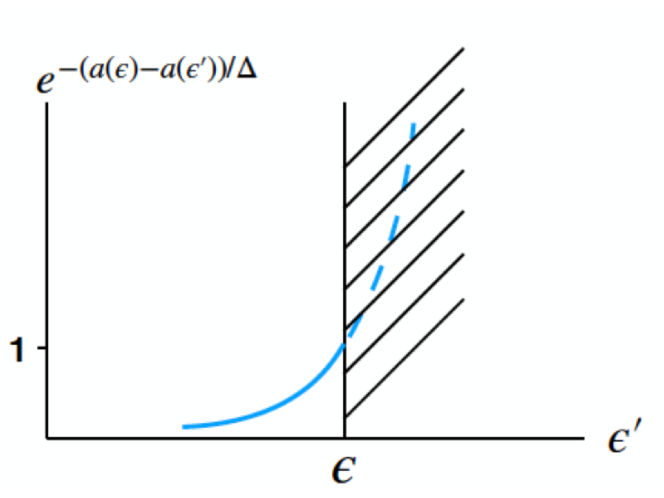
Figure 7: This is a plot of the integrand $\exp(-(a(\epsilon)-a(\epsilon^{\prime}))/\Delta)$ as a function of $\epsilon^{\prime}$ in the expression (156) for the stationary distribution $P_{0}(\epsilon)$.

In the exponent $a(\epsilon)=2(\epsilon^{3}/3+(m/\langle\kappa\rangle)\omega^{2}\epsilon)$ is a monotonically increasing function passing through the origin. A plot of $\exp(-(a(\epsilon)-a(\epsilon^{\prime}))/\Delta)$ is schematically depicted in Fig. 7. For small $\Delta$ the exponential function rises steeply and the main contribution to $P(\epsilon)$ arises from the region $\epsilon^{\prime}\leq\epsilon$. To leading order a steepest descent argument yields $P_{0}^{(1)}=C/a^{\prime}$. The next term in the asymptotic expansion is obtained by expanding $a(\epsilon^{\prime})$, i.e., $a(\epsilon^{\prime})=a(\epsilon)+a^{\prime}(\epsilon)(\epsilon^{\prime}-\epsilon)+(1/2)a^{\prime\prime}(\epsilon)(\epsilon^{\prime}-\epsilon)^{2}$. A straightforward calculation then yields $P_{0}^{(2)}=Ca^{\prime\prime}/a^{\prime 3}$. In conclusion, the expansion in (48) is an asymptotic expansion in $\Delta$, i.e., the leading correction to the steepest descent term.

VIII.3 Heat current

Focussing on the heat reservoir at temperature $T_{1}$ at the site $n=1$, the integrated heat flux is obtained from (7), i.e.,

$$Q(t)=\int^{t}dt^{\prime}F_{1}(t^{\prime})\dot{u}_{1}(t^{\prime}).$$ (157)

Inserting $F_{1}=-\Gamma\dot{u}_{1}+\xi_{1}$ and $u_{1}$ from (12) we obtain in Fourier space

$$Q(t)=\int\frac{d\omega}{2\pi}\frac{d\omega^{\prime}}{2\pi}F(\omega-\omega^{\prime},t)\left(\begin{array}[]{cc}\tilde{\xi}_{1}(\omega)&\tilde{\xi}_{2}(\omega)\end{array}\right)M(\omega,\omega^{\prime})\left(\begin{array}[]{c}\tilde{\xi}_{1}(\omega^{\prime})\\ \tilde{\xi}_{2}(\omega^{\prime})\end{array}\right),$$ (161)

where the matrix elements of $M$ are given by

$$M_{11}(\omega,\omega^{\prime})=-\omega\omega^{\prime}\Gamma G_{11}(\omega)G_{11}(-\omega^{\prime})+\frac{1}{2}\bigg{(}-i\omega G_{11}(\omega)+i\omega^{\prime}G_{11}(-\omega^{\prime})\bigg{)},$$ (162)

$$M_{22}(\omega,\omega^{\prime})=-\omega\omega^{\prime}\Gamma G_{1N}(\omega)G_{1N}(-\omega^{\prime}),$$ (163)

$$M_{12}(\omega,\omega^{\prime})=-\omega\omega^{\prime}\Gamma G_{11}(\omega)G_{1N}(-\omega^{\prime})+\frac{1}{2}i\omega^{\prime}G_{1N}(-\omega^{\prime}),$$ (164)

$$M_{21}(\omega,\omega^{\prime})=-\omega\omega^{\prime}\Gamma G_{1N}(\omega)G_{11}(-\omega^{\prime})-\frac{1}{2}i\omega G_{1N}(\omega).$$ (165)

The function $F(\omega,t)=2\sin(\omega t/2)\exp(-i\omega t/2)/\omega$. Moreover, $F(0,t)=t$ and $|F(\omega,t|^{2}=2\pi t\delta(\omega)$ for large $t$. Finally, using the noise correlations (5) and (6) and the Schwinger identity (81), we obtain the mean heat flux $J=\langle Q(t)\rangle/t$ in (57), i.e.,

$$J=2(T_{1}-T_{2})\int\frac{d\omega}{2\pi}(\omega\Gamma)^{2}|G_{1N}(\omega)|^{2}.$$ (166)

VIII.4 Large deviation function

The large deviation function function is defined according to

$$\mu(\lambda)=\lim_{t\rightarrow\infty}\frac{1}{t}\ln\langle\exp(\lambda Q(t))\rangle,$$ (167)

where $Q(t)$ is given by (161). Inserting $Q(t)$, using the noise distribution

$$P(\xi_{1},\xi_{2})\propto\exp\Bigg{[}-\frac{1}{2}\int\frac{d\omega}{2\pi}\frac{d\omega^{\prime}}{2\pi}\left(\begin{array}[]{cc}\xi_{1}(\omega)&\xi_{2}(\omega)\end{array}\right)\Delta^{-1}(\omega-\omega^{\prime})\left(\begin{array}[]{c}\xi_{1}(\omega^{\prime})\\ \xi_{2}(\omega^{\prime})\end{array}\right)\Bigg{]},$$ (171)

where the inverse noise matrix is

$$\Delta^{-1}(\omega-\omega^{\prime})=\left(\begin{array}[]{cc}\Delta^{-1}_{1}&0\\ 0&\Delta^{-1}_{2}\end{array}\right)\delta(\omega-\omega^{\prime}),$$ (174)

with $\Delta_{1}=2\Gamma T_{1}$ and $\Delta_{2}=2\Gamma T_{2}$, and using the matrix identity Zinn-Justin (1989)

$$\langle\exp(-(1/2\tilde{\xi}B\xi)\rangle=\exp(\rm{Tr}\ln(I+\Delta B)),$$ (175)

we obtain formally

$$\mu(\lambda)=-\frac{1}{2t}\rm{Tr}\ln(I+2\lambda F\Delta M);$$ (176)

we note that formula (175) follows from (1.5) in Ref. Zinn-Justin (1989) setting $b_{i}=0$ and using $\text{det}A=\exp(\text{Tr}\log A)$.

Using the properties of $F$, the limits for $\omega=\omega^{\prime}$

$$M_{11}(\omega,\omega)=-M_{22}(\omega,\omega)=\omega^{2}\Gamma|G_{1N}(\omega)|^{2},$$ (177)

$$M_{12}(\omega,\omega)=M_{21}(\omega,\omega)^{\ast}=-\omega^{2}\Gamma G_{11}(\omega)G_{1N}(\omega)^{\ast}+(1/2)i\omega G_{1N}(\omega)^{\ast},$$ (178)

the Schwinger identity (81), and diagonalising $\Delta M$, we obtain the eigenvalue equation for the eigenvalues $\alpha_{1}(\omega)$ and $\alpha_{2}(\omega)$

$$\alpha^{2}-2\Gamma\alpha(T_{1}M_{11}+T_{2}M_{22})+4\Gamma^{2}T_{1}T_{2}(M_{11}M_{22}-M_{12}M_{21})=0.$$ (179)

For $\mu$ we then obtain

$$\mu(\lambda)=-\frac{1}{2}\int\frac{d\omega}{2\pi}\ln(1-2\lambda(\alpha_{1}+\alpha_{2})+4\lambda^{2}\alpha_{1}\alpha_{2}),$$ (180)

or reduced further the final result

$$\mu(\lambda)=-\frac{1}{2}\int\frac{d\omega}{2\pi}\ln(1+4\omega^{2}\Gamma^{2}|G_{1N}(\omega)|^{2}f(\lambda)),$$ (181)

where

$$f(\lambda)=T_{1}T_{2}\lambda(1/T_{1}-1/T_{2}-\lambda).$$ (182)

References

- Trepagnier et al. (2004) E. Trepagnier, C. Jarzynski, F. Ritort, G. Crooks, C. Bustamante, and J. Liphardt, Proc. Natl. Acad. Sci. USA 101, 15038 (2004).
- Collin et al. (2005) D. Collin, F. Ritort, C. Jarzynski, S. B. Smith, I. T. Jr, and C. Bustamante, Nature 437, 231 (2005).
- Tietz et al. (2006) C. Tietz, S. Schuler, T. Speck, U. Seifert, and J. Wrachtrup, Phys. Rev. Lett. 97, 050602 (2006).
- Blickle et al. (2006) V. Blickle, T. Speck, L. Helden, U.Seifert, and C. Bechinger, Phys. Rev. Lett. 96, 070603 (2006).
- Imparato et al. (2007) A. Imparato, L. Peliti, G. Pesce, G. Rusciano, and A. Sasso, Phys. Rev. E 76, 050101R (2007).
- Douarche et al. (2006) F. Douarche, S. Joubaud, N. B. Garnier, A. Petrosyan, and S. Ciliberto, Phys. Rev. Lett. 97, 140603 (2006).
- Garnier and Ciliberto (2007) N. Garnier and S. Ciliberto, Phys. Rev. E 71, 060101(R) (2007).
- Imparato et al. (2008) A. Imparato, P. Jop, A. Petrosyan, and S. Ciliberto, J. Stat. Mech p. P10017 (2008).
- Jarzynski (1997) C. Jarzynski, Phys. Rev. Lett. 78, 2690 (1997).
- Kurchan (1998) J. Kurchan, J. Phys. A 31, 3719 (1998).
- Gallavotti (1996) G. Gallavotti, Phys. Rev. Lett. 77, 4334 (1996).
- Crooks (1999) G. E. Crooks, Phys. Rev. E 60, 2721 (1999).
- Crooks (2000) G. E. Crooks, Phys. Rev. E 61, 2361 (2000).
- Seifert (2005a) U. Seifert, Phys. Rev. Lett. 95, 040602 (2005a).
- Seifert (2005b) U. Seifert, Europhys. Lett 70, 36 (2005b).
- Evans et al. (1993) D. J. Evans, E. G. D. Cohen, and G. P. Morriss, Phys. Rev. Lett. 71, 2401 (1993).
- Evans and Searles (1994) D. J. Evans and D. J. Searles, Phys. Rev. E 50, 1645 (1994).
- Gallavotti and Cohen (1995) G. Gallavotti and E. G. D. Cohen, Phys. Rev. Lett. 74, 2694 (1995).
- Lebowitz and Spohn (1999) J. L. Lebowitz and H. Spohn, J. Stat. Phys. 95, 333 (1999).
- Gaspard (2004) P. Gaspard, J. Stat. Phys. 117, 599 (2004).
- Imparato and Peliti (2006) A. Imparato and L. Peliti, Phys. Rev. E 74, 026106 (2006).
- van Zon and Cohen (2003a) R. van Zon and E. G. D. Cohen, Phys. Rev. Lett. 91, 110601 (2003a).
- van Zon et al. (2004) R. van Zon, S. Ciliberto, and E. G. D. Cohen, Phys. Rev. Lett. 92, 130601 (2004).
- van Zon and Cohen (2003b) R. van Zon and E. G. D. Cohen, Phys. Rev. E 67, 046102 (2003b).
- van Zon and Cohen (2004) R. van Zon and E. G. D. Cohen, Phys. Rev. E 69, 056121 (2004).
- Speck and Seifert (2005) T. Speck and U. Seifert, Eur. Phys. J. B 43, 521 (2005).
- Bonetto et al. (2000) F. Bonetto, J. L. Lebowitz, and L. Rey-bellet, in Mathematical Physics 2000 (World Scientific, Singapore, 2000), pp. 128–150.
- Jackson (1978) E. A. Jackson, Rocky Mountain J. Math. 8, 127 (1978).
- Dhar (2008) A. Dhar, Adv. Phys. 57, 457 (2008).
- Lepri et al. (2003) S. Lepri, R. Livi, and A. Politi, Phys. Rep. 377, 1 (2003).
- Dhar and Saitou (2016) A. Dhar and K. Saitou, Lecture Notes in Physics 921 (2016).
- Ajanki and Huveneers (2011) O. Ajanki and F. Huveneers, Communications in Mathematical Physics 301, 841 (2011).
- Ash et al. (2020) B. Ash, A. Amir, Y. Bar-Sinai, Y. Oreg, and Y. Imry, Phys. Rev. B 101, 121403(R) (2020).
- Ong and Zhang (2014) Z.-Y. Ong and G. Zhang, J. Phys Condens Matter 26(33), 335402 (2014).
- Yamada (2018) H. S. Yamada, Chaos, Solitons and Fractals 113, 178 (2018).
- Amir et al. (2018) A. Amir, Y. Oreg, and Y. Imry, Europhys. Lett 124, 16001 (2018).
- Herrera-Gonzalez et al. (2010) I. F. Herrera-Gonzalez, F. M. Izrailev, and L. Tessieri, Europhys. Lett 90, 14001 (2010).
- Herrera-Gonzalez et al. (2015) I. F. Herrera-Gonzalez, F. M. Izrailev, and L. Tessieri, Europhys. Lett 110, 64001 (2015).
- Herrera-Gonzalez and Mendez-Bermudez (2019) I. F. Herrera-Gonzalez and J. A. Mendez-Bermudez, Phys. Rev. E 100, 052109 (2019).
- Zhou et al. (2016) H. Zhou, G. Zhang, J.-S. Wang, and Y.-W. Zhang, Phys. Rev. E 94, 052123 (2016).
- Kundu (2010) A. Kundu, Phys. Rev. E 82, 031131 (2010).
- Saito and Dhar (2011) K. Saito and A. Dhar, Phys. Rev. E 83, 041121 (2011).
- Kundu et al. (2011) A. Kundu, S. Sabhapandit, and A. Dhar, J. Stat. Mech. p. P03007 (2011).
- Fogedby and Imparato (2012) H. C. Fogedby and A. Imparato, J. Stat. Mech. p. P04005 (2012).
- Casher and Lebowitz (1971) A. Casher and J. L. Lebowitz, J. Math. Phys. 12, 1701 (1971).
- Dhar and Lebowitz (2008) A. Dhar and J. L. Lebowitz, Phys. Rev. Lett. 100, 134301 (2008).
- Dhar et al. (2011) A. Dhar, K. Venkateshan, and J. L. Lebowitz, Phys. Rev. E 83, 021108 (2011).
- Kundu et al. (2010) A. Kundu, A. Chaudhuri, D. Roy, A. Dhar, J. L. Lebowitz, and H. Spohn, Europhys. Lett 90, 40001 (2010).
- Chaudhuri et al. (2010) A. Chaudhuri, A. Kundu, D. Roy, A. Dhar, J. L. Lebowitz, and H. Spohn, Phys. Rev. B 81, 064301 (2010).
- Lee and Dhar (2005) L. W. Lee and A. Dhar, Phys. Rev. Lett. 95, 094302 (2005).
- O’Connor and Lebowitz (1974) A. J. O’Connor and J. L. Lebowitz, J. Math. Phys. 15, 692 (1974).
- Roy and Dhar (2008a) D. Roy and A. Dhar, J. Stat. Phys. 131, 535 (2008a).
- Roy and Dhar (2008b) D. Roy and A. Dhar, Phys. Rev. E 78, 051112 (2008b).
- Anderson (1958) P. W. Anderson, Phys. Rev. 109, 1492 (1958).
- Matsuda (1962) H. Matsuda, Prog. Theo. Phys. (Suppl.) 23, 22 (1962).
- Matsuda and Ishii (1970) H. Matsuda and K. Ishii, Prog. Theo. Phys. (Suppl.) 45, 56 (1970).
- Ishii (1973) K. Ishii, Prog. Theo. Phys. (Suppl.) 53, 77 (1973).
- Saito and Dhar (2007) K. Saito and A. Dhar, Phys. Rev. Lett. 99, 180601 (2007).
- Dhar (2001) A. Dhar, Phys. Rev. Lett. 86, 5882 (2001).
- Furstenberg (1963) H. Furstenberg, Trans. Amer. Math. Soc. 108, 377 (1963).
- O’Connor (1975) A. J. O’Connor, Commun. math. Phys. 45, 63 (1975).
- Reichl (1998) L. E. Reichl, A Modern Course in Statistical Physics (Wiley, New York, 1998).
- Matsuda et al. (1968) H. Matsuda, T. Miyata, and K. Ishii, Suppl. J. Phys. Soc. Japan 26, 40 (1968).
- Jackson (1990) E. Jackson, Perspectives of nonlinear dynamics (Cambridge University Press, Cambridge, 1990).
- Risken (1989) H. Risken, The Fokker-Planck Equation (Springer-Verlag, Berlin, 1989).
- Nieuwenhuizen (1983) T. M. Nieuwenhuizen, Physica A 120A, 468 (1983).
- Lifshits et al. (1988) I. Lifshits, S. Gredeskul, and L. Pasteur, Introduction to the Theory of Disordered Systems (Wiley, New York, 1988).
- Luck (2004) J. M. Luck, J. Phys. A 37, 259 (2004).
- Grabsch et al. (2014) A. Grabsch, C. Texier, and Y. Tourigny, J. Stat. Phys. 155, 237 (2014).
- Rubin and Greer (1971) R. J. Rubin and W. L. Greer, J. Math. Phys. 12, 1686 (1971).
- Dhar and Roy (2006) A. Dhar and D. Roy, J. Stat. Phys. 125, 805 (2006).
- Touchette (2009) H. Touchette, Phys. Rep. 478, 1 (2009).
- den Hollander (2000) F. den Hollander, Large Deviations, vol. 14 (American Mathematical Society, Providence, R.I., 2000).
- Fogedby and Imparato (2011) H. C. Fogedby and A. Imparato, J. Stat. Mech. p. P05015 (2011).
- Fogedby and Imparato (2014) H. C. Fogedby and A. Imparato, J. Stat. Mech. p. P11011 (2014).
- Wang and Uhlenbeck (1945) M. C. Wang and G. E. Uhlenbeck, Rev. Mod. Phys 17, 323 (1945).
- Lebedev (1972) N. N. Lebedev, Special functions and their applications (Dover Publications, New York, 1972).
- Zinn-Justin (1989) J. Zinn-Justin, Quantum Field Theory and Critical Phenomena (Oxford University Press, Oxford, 1989).