A universal neural network for learning phases and criticalities

Abstract

A universal supervised neural network (NN) relevant to compute the associated criticalities of real experiments studying phase transitions is constructed. The validity of the built NN is examined by applying it to calculate the criticalities of several three-dimensional (3D) models on the cubic lattice, including the classical $O(3)$ model, the 5-state ferromagnetic Potts model, and a dimerized quantum antiferromagnetic Heisenberg model. Particularly, although the considered NN is only trained one time on a one-dimensional (1D) lattice with 120 sites, yet it has successfully determined the related critical points of the studied 3D systems. Moreover, real configurations of states are not used in the testing stage. Instead, the employed configurations for the prediction are constructed on a 1D lattice of 120 sites and are based on the bulk quantities or the microscopic states of the considered models. As a result, our calculations are ultimately efficient in computation and the applications of the built NN is extremely broaden. Considering the fact that the investigated systems vary dramatically from each other, it is amazing that the combination of these two strategies in the training and the testing stages lead to a highly universal supervised neural network for learning phases and criticalities of 3D models. Based on the outcomes presented in this study, it is favorably probable that much simpler but yet elegant machine learning techniques can be constructed for fields of many-body systems other than the critical phenomena.

Introduction — Techniques from machine learning (ML), which originally belong to the fields of information and computer sciences, have found applications in many-body systems during the last a few years Rup12 ; Sny12 ; Li15 ; Baldi:2014pta ; Mnih:2015jgp ; Searcy:2015apa ; Baldi:2016fzo ; Baldi:2016fql ; Tor16 ; Wan16 ; Att16 ; Oht16 ; Hoyle:2015yha ; Car16 ; Tro16 ; Bro16 ; Chn16 ; Tan16 ; Tubiana:2016zpw ; Nie16 ; Mott:2017xdb ; Liu16 ; Tam17 ; Xu16 ; Wan17 ; Liu17 ; Nag17 ; Kol17 ; Den17 ; Zha17 ; Zha17.1 ; Hu17 ; Li18 ; Chn18 ; Lu18 ; Bea18 ; Pang:2016vdc ; Sha18 ; But18 ; Bar18 ; Zha18 ; Butter:2017cot ; Gao18 ; Zha19 ; Gre19 ; Ren:2017ymm ; Don19 ; Cavaglia:2018xjq ; Dav19 ; Conangla:2018nnn ; Li19 ; Lia19 ; Meh19 ; Rod19 ; Car19 ; Oht20 ; Larkoski:2017jix ; Han:2019wue ; Tan20.1 ; Tan20.2 ; Sin20 ; Lidiak:2020vgk ; Carrasquilla:2020mas ; Wan20 ; Son20 ; Cao:2020rgr ; Amacker:2020bmn ; Bachtis:2020dmf ; Aad:2020cws ; Beentjes:2020abj ; Morgan:2020wvf ; Shalloo:2020nhu ; Tomita:2020ylz ; Cabero:2020eik ; Geilhufe:2020nbl ; Wang:2020tgb ; Nicoli:2020njz . Such examples include studies associated with the critical phenomena, the high energy particle physics, and the first principles material calculations. In some cases, the performance of these new approaches for exploring many-body physical systems is comparable with that of the traditional methods.

While applying the ML techniques to investigate physical systems has been developed for some time and many promising achievements are obtained, research activities on improving the efficiency of those ML methods are still vigorous. Taking topological phase transition for example, both the supervised and the unsupervised neural networks (NN) are adopted to study this kind of exotic criticality. Although many attempts have been done and satisfactory outcomes are reached, there is still some room for improvement.

Indeed, the accomplishments of employing the NN methods to explore the criticalities of many-body systems are typically achieved using very complicated infrastructures such as the convolutional neural networks (CNN). Specially, a convolutional layer, which is intended to capture certain characteristics of the considered system, is included in the CNN. From this point of view, an investigation on the targeted system somehow is required before one can build a appropriate CNN to study the associated criticality. In other words, a constructed CNN for a particular model may not be applicable for another one. In particular, redesigning a relevant convolutional layer is needed whenever a new and completely different system is considered.

Apart from the complications introduced in the previous paragraph, in the training stage of a NN calculation, few to several thousand real configurations generated by some (numerical) methods are used as the training set typically. Moreover, each of the system sizes used in the calculations requires one separate training as well. This described training procedure is time consuming and may use up a lot of computing resources. Besides, the majority of NN calculations for studying critical phenomena also employ real configurations of states in the testing (prediction) stage. Such a strategy in the testing stage take huge amount of storage space if system(s) of large sizes are considered, and it may not directly applicable to some results obtained from experiments. This is because in many cases it is the bulk properties, not the detailed states of the studied materials, is measured and recorded in the laboratories. As a result, it will be highly desirable to construct a NN with an infrastructure that can simplify the training procedure and make a closer connection to the reality conducted in experiments.

As demonstrated in Refs. Li18 ; Tan20.1 , when studying the phase transitions of the $q$-state ferromagnetic Potts models with a NN, the consideration of using the theoretical ground state configurations in the ordered phase as the training sets greatly reduces the needed computations for the training. Later a training strategy of using only two configurations made artificially can even detect the critical points with high accuracy for the three-dimensional (3D) classical $O(3)$ models, the two-dimensional (2D) $XY$ models, and the 3D and 2D dimerized quantum antiferromagnetic Heisenberg models Tan20.2 . The outcomes shown in Ref. Tan20.2 indicate that little information of the underlying systems is sufficient to uncover the critical phenomena of these considered models. This is quite surprising, considering the fact that these studied models have infinite number degree of freedom. Moreover, it is amazing as well that such a simple training procedure is valid for models that are different dramatically from each other.

Despite the remarkable achievements, one training is still needed for every considered system size for the NN calculations carried out in Ref. Tan20.2 . In addition, real configurations of states of the studied models are stored and employed in the testing stage as well. As pointed out previously, this does not match very well with many real experimental situations, since typically the bulk quantities rather than the detailed microscopic details are available in experiments. Here we demonstrate that it is possible to build a simple supervised NN that is relevant to compute the associated criticalities of real experiments studying phase transitions. Moreover, the NN is obtained by carrying out only one training on a fixed size one-dimensional (1D) lattice, and the validity of the resulting NN is examined by applying it to calculate the critical points of various models with many system sizes. Specifically, we train a MLP (defined later) on a 1D lattice of 120 sites and successfully employ the obtained weight to calculate the critical points of the 3D classical $O(3)$ model, a 3D dimerized quantum antiferromagnetic Heisenberg model (abbreviated as the plaquette model here), and the 3D 5-state ferromagnetic Potts model. Moreover, instead of using the configurations of states directly determined from the simulations, in the prediction stage, the configurations employed are constructed based on some bulk quantities of the considered models having certain characteristics (These characteristics will be detailed in the relevant sections). Such a strategy for the testing stage is not only economically efficient in storage, but is also close to the situations of real experiments, namely only the bulk quantities are recorded. As a result, the procedures of the NN calculations presented here are directly applicable for the relevant experiments.

Considering the fact that the majority of applying ML methods to study many-body systems use real microscopic configurations for the prediction stage, here we also construct configurations on a 1D lattice of 120 sites based on the microscopic states of the studied systems. It turns out that this second method of building the configurations for the NN prediction leads to successful outcomes as well.

It is beyond one’s intuition and is surprisingly impressive that a NN determined on a fixed 1D lattice can be used to study the criticalities of several 3D models of various system sizes. In particular, these studied 3D systems are dramatically different among themselves. Finally, in conjunction with the data obtained from the relevant experiments, our approach is perfectly suitable for studying the associated phases and criticalities.

The constructed supervised Neural Network — In this section, we review the supervised NN, namely the multilayer perceptron (MLP) used in our study. The employed training set and label will be introduced as well. Part of this section is a short summary of that in Refs. Tan20.1 ; Tan20.2 .

The MLP used in our investigation is already detailed in Ref. Tan20.1 ; Tan20.2 . Specifically, using the NN library keras and tensorflow kera ; tens , we construct a supervised NN which consists of only one input layer, one hidden layer of 512 independent nodes, and one output layer. In addition, The algorithm, optimizer, and loss function considered in our calculations are the minibatch, the adam, and the categorical cross entropy, respectively. To avoid overfitting, we also apply $L_{2}$ regularization at various stages. The activation functions employed here are ReLU and softmax. The details of the constructed MLP, including the steps of one-hot encoding and flatten (and how these two processes work) are shown in the supplemental materials and are available in Refs. Tan20.1 ; Tan20.2 .

Finally, for the three studied models, results calculated using 10 sets of random seeds are all taken into account when presenting the final outcomes. Specifically, each set of random seeds leads to a mean resulting from a few hundred to several thousand (independent) outcomes. The final quote values are then based on the mean and the standard deviation of these 10 mean results.

For the training set and the associated training procedure carried out in our NN calculations, a simple alternative is considered. Specifically, instead of using real configurations obtained from the simulations or the theoretical ground states in the ordered phase of the studied system(s), only one training on a 120 sites one-dimensional (1D) lattice is conducted. In addition, the training set consists of two configurations. Particularly, one of the configuration has 0 as the value for each of its site, and every spot of the other configuration takes the number of 1. Consequently, the output labels are naturally the vectors of $(1,0)$ and $(0,1)$.

In this study, instead of using real configuration of states for the testing (prediction), bulk quantities are considered. Based on the fact that physical observables which take distinct values at different phases is essential to distinguish various states, we use a criterion to choose the relevant bulk quantities to construct configurations for the testing (prediction). Specifically, in the simulated range of $T$ (or other relevant parameters) the chosen observable(s) should saturate to distinct values at the high and the low temperature regions. We find that the Binder ratios $Q_{1}$ and $Q_{2}$ suit this criterion very well. After a desired observable $O$ is picked, one carries out the associated simulations with many different inverse temperatures $\beta$ and on lattices of various linear sizes $L$. For each $L$ the difference of $O$ at the highest and the lowest temperatures is recorded. Let this quantity be denoted by $D_{O,L}$. Then for the same observable at every other temperature, a configuration on a 1D lattice of 120 sites, which will be used to feed the trained NN, is constructed through the following steps.

1. For a given temperature $T_{m}$, let the difference between the values of $O$ at $T_{m}$ and that at the lowest temperature be $D_{m}$.

2. For each site $i$ of the 1D lattice, choose a number $p$ in [0,1) randomly and uniformly.

3. If $p\geq|D_{m}/D_{O,L}|$, then the site $i$ is assigned the integer $1$. Otherwise the integer $0$ is given to $i$.

4. Repeat above steps for all the simulated (inverse) temperatures.

The configurations constructed from these described steps, which are based on the bulk quantities of the studied models, are then fed to the trained NN. With this set up, the associated critical point can be estimated by investigating the temperature (or other relevant tuning parameter) dependence of the output vectors $\vec{V}$. In particular, when those $\vec{V}$ are considered as functions of $\beta$, the critical point is located at the inverse temperature corresponding to the intersections of the two curves made up from the components of $\vec{V}$. It should be pointed out that, the critical point may be also obtained as the (inverse) temperature associated with the output which has the smallest value of magnitude.

We would like to emphasize the fact that technically speaking, only one training on a pre-chosen 1D lattice using two objects as the training set is conducted here. The resulting weight is then used to perform the NN prediction for all the studied 3D models with various system sizes. Hence the training process takes much less computing resources than (any) other known schemes in the literature. Moreover, no real configuration of states are used in the testing stage, and only bulk quantities fulfilling certain properties are recorded. As a result, the required storage is also much smaller when compared with other methods of studying phases and criticalities using the NN approaches.

Despite its simplicity in the training as well as the testing stages, as we will demonstrate later, the trained NN is capable of detecting the critical points of all the considered models with high accuracy.

Apart from the constructed 1D configurations introduced above, based on the microscopic states of the studied systems, configurations on a 1D lattice of 120 sites are built additionally and are used for the NN prediction as well. This second method for the testing stage leads to successful calculations as well. The details of this second construction will be presented in the supplemental materials.

The numerical results — In this section, results obtained by using the constructed NN will be presented. The needed Monte Carlo simulations are performed using the Wolff algorithm Wol89 and the stochastic series expansion algorithm with operator-loop update San99 .

As mentioned earlier, for all the three studied 3D models, we find the first and the second Binder ratios ($Q_{1}$ and $Q_{2}$) suit the criterion introduced previously. After the appropriate observables are determined, two types of configurations used for the testing (prediction) are constructed according to the rules outlined in the previous section and the supplemental materials.

The observable $Q_{2}$ (obtained on a $48^{3}$ cubic lattice) as a function of $\beta$ for the 3D classical $O(3)$ model is shown in fig. 1. Although the outcomes in fig. 1 indicate that $T_{c}$ lies between $\beta=0.67$ and $\beta=0.71$, it can not determined directly from the results in the figure.

The norm $R$ (associated with $Q_{2}$ obtained on a $48^{3}$ lattice) of the outputs, which are determined by using the NN weight obtained from the calculation of employing only two training objects on a 1D lattice of $L=120$, are shown in fig. 2. As can be seen from the figure, the minimum of $R$ takes place at a $\beta$ very close to the critical inverse temperature $\beta_{c}$ (dashed vertical lines) of the considered 3D classical $O(3)$ model. Moreover, the $\beta$ dependence of individual component $V_{1}$ and $V_{2}$ of the output vectors $\vec{V}$ are demonstrated in fig. 3. Similar to the scenario of $R$, the intersection of the $V_{1,2}$ v.s. $\beta$ curves is very close to $\beta_{c}$ as well. The results in fig. 2 and 3 confirm the validity of our NN approach outlined in the previous sections.

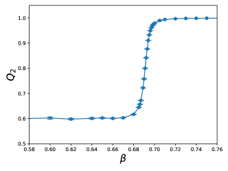
Figure 1: $Q_{2}$ (on $48^{3}$ cubic lattices) as a function of $\beta$ for the 3D classical $O(3)$ model.

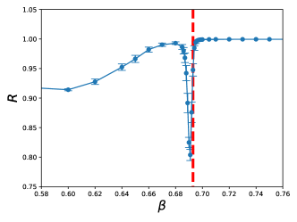
Figure 2: $R$ as a function of $\beta$ for the 3D classical $O(3)$ model. The dashed line is the expected $\beta_{c}$. The results are associated with $Q_{2}$ (on $48^{3}$ cubic lattices).

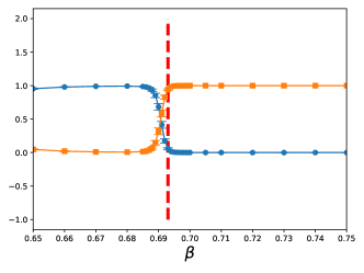
Figure 3: Individual component of the output vectors as functions of $\beta$ for the 3D classical $O(3)$ model. The results are related to the observable $Q_{2}$ (on $48^{3}$ cubic lattices). The dashed line is the expected $\beta_{c}$.

Similar scenarios are observed for the 3D 5-state ferromagnetic Potts model and the 3D dimerized quantum plaquette model, see the supplemental materials.

Finally, configurations on a 1D lattice of 120 sites using the microscopic classical $O(3)$ spin states obtained from the simulations are built and are used for the prediction. We first randomly and uniformly pick up 120 sites of the spin states and then follow the procedures outlined in Ref. Tan20.2 to construct the associated configurations for the prediction. It turns out that this second approach leads to high precision determination of the critical point(s) as well, see fig. 4 and the supplemental materials.

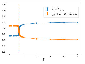
Figure 4: $R+\Delta$ and $1/\sqrt{2}+1-R-\Delta$ as functions of $\beta$ for the 3D classical $O(3)$ model. The dashed line is the expected $\beta_{c}$. The outcomes are associated with the spin configurations on $24^{3}$ lattices. The definitions of $R$ and $\Delta$ can be found in Ref. Tan20.2 .

Discussions and Conclusions — In this study, we calculate the critical points associated with the 3D classical $O(3)$ model, the 3D 5-state ferromagnetic Potts model, and a 3D dimerized quantum antiferromagnetic Heisenberg model, using the technique of supervised Neural Networks. Particularly, unlike any NN studies known in the literature, an extremely simple built NN as well as elegant training and testing procedures are adopted in our investigation.

In our approach for the training stage, only one training using two configurations on a fixed size (120) 1D lattice is conducted. The resulting weight is then applied to calculate the critical points of three 3D systems. In the testing (prediction) stage, not the real configurations, but the configurations constructed based on the bulk observables which have certain characteristics are employed to feed the trained NN. The combination of such two strategies for the training and the testing stages are not only highly efficient in computation, but also determine accurately the critical points of the considered 3D models. Apart from this extremely efficient approach, we also construct configurations on a 1D lattice of 120 sites based on the microscopic spin states for the prediction. The second method leads to successful determination of the targeted critical point(s) as well.

Although the nature and the degree of freedom of the three considered models vary dramatically from each other, it is remarkable that the constructed NN is applicable for all of these cases. Specially, it is amazing the weight obtained by carrying out only one training procedure on a 1D lattice with fixed size can be employed successfully to calculate the critical points associated with various 3D models. Here we would like to emphasize the fact that it seems flexible to choose a lattice of any dimension and size for the training. Indeed, as we will shown in the supplemental materials, the targeted critical points can be determined precisely using a NN trained on a 1D lattice of 200 sites as well as a 2D square lattice with linear system size $L=16$.

When compared with other NN schemes, our approach is highly advanced in both the efficiency and the simplicity. Some benchmarks are provided in the supplemental materials. In reality, bulk quantities are measured in many experiments. Hence the use of employing bulk observables to build the associated configurations to feed the trained NN makes the approach presented here more attractive since it is directly applicable to the data obtained from the relevant experiments.

Finally, according to our series of studies regarding improving the efficiency of applying the supervised NN to investigate the phase transitions Li18 ; Tan20.1 ; Tan20.2 , it is probable that with some elegant ideas, much more efficient machine learning methods for studying many-body physical problems other than the critical phenomena can be obtained.

Partial support from Ministry of Science and Technology of Taiwan is acknowledged.

Supplemental materials

For the benefit of readers, in this supplemental materials, the constructed NN, the studied models, and more results are presented. We would like to emphasize the fact that part of this supplemental materials are available in Refs. Li18 ; Tan20.1 ; Tan20.2 .

The constructed NN — The built NN mentioned in the main text consists of only one input layer, one hidden layer of 512 nodes, and one output layer. Figure 5 represents the infrastructure of the NN (MLP) employed in this investigation. For the reader who are interested in the details of the considered NN (MLP) shown in fig. 5, including the used algorithms, the optimization, the activation functions ReLU and softmax, and the loss function categorical crossing entropy, are referred to Ref. Tan20.2 .

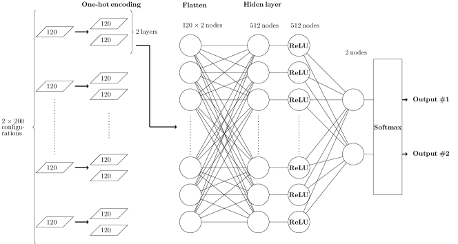
Figure 5: The NN (MLP), which consists of one input layer, one hidden layer, and one output layer, used here and in Refs. Tan20.1 ; Tan20.2 . The objects in the input layer are made up of 200 copies of only two configurations. There are 512 nodes in the hidden layer and each of these nodes is independently connected to every object in the input layer. Before each training object is connected to the nodes in the hidden layer, the steps of one-hot encoding and flatten are applied. The activation functions (ReLU and softmax) and where they are employed are demonstrated explicitly. Finally, the output layers consist of two elements.

The microscopic models and observables — The models considered in this study have been investigated extensively in the literature. Here we summarize the associated Hamiltonians and the observables that are relevant to our study. Some of these descriptions have been appeared in Refs. Li18 ; Tan20.1 ; Tan20.2 . — The 3D classical $O(3)$ (Heisenberg) model Tan20.2 —

The Hamiltonian $H_{O(3)}$ of the 3D classical $O(3)$ (Heisenberg) model on a cubic lattice considered in our study is given by

$$\beta H_{O(3)}=-\beta\sum_{\left<ij\right>}\vec{s}_{i}\cdot\vec{s}_{j},$$ (1)

where $\beta$ is the inverse temperature and $\left<ij\right>$ stands for the nearest neighbor sites $i$ and $j$. In addition, in Eq. (1) $\vec{s}_{i}$ is a unit vector belonging to a 3D sphere $S^{3}$ and is located at site $i$.

Relevant observables used in this study are the first and the second Binder ratios ($Q_{1}$ and $Q_{2}$) which are given as

$$Q_{1} = \langle|m|\rangle^{2}/\langle m^{2}\rangle,$$ (2)

$$Q_{2} = \langle m^{2}\rangle^{2}/\langle m^{4}\rangle,$$ (3)

where $m=\frac{1}{L^{3}}\sum_{i}\vec{s}_{i}$ and $L$ is the linear box size of the system Bin81 . — The 3D dimerized quantum antiferromagnetic Heisenberg models Tan20.2 —

The 3D dimerized quantum antiferromagnetic Heisenberg model has the following expression as its Hamiltonian

$$H=\sum_{\langle i,j\rangle}J_{ij}\vec{S}_{i}\cdot\vec{S_{j}},$$ (4)

where again $\langle i,j\rangle$ stands for the nearest neighbor sites $i$ and $j$, $J_{ij}>0$ is the associated antiferromagnetic coupling (bond) connecting $i$ and $j$, and $\vec{S}_{i}$ is the spin-1/2 operator located at $i$. The cartoon representation of the studied model is shown in fig. 6 and this model will be named 3D plaquette model here if no confusion arises. Moreover, in the figure, the antiferromagnetic couplings for the thick and thin bonds are $J^{\prime}$ and $J$, respectively. Based on fig. 6, one sees that as the magnitude of $g$ (Which is defined as $J^{\prime}/J$) increases, a quantum phase transition from the ordered to the disordered states will occur once $g$ exceeds a particular value $g_{c}$. Relevant observables considered in our investigation for studying the quantum phase transition are again the first and the second Binder ratios $Q_{1}$ and $Q_{2}$. For the studied spin-1/2 system, $Q_{1}$ and $Q_{2}$ have the following definitions

$$Q_{1} = \langle|M_{s}|\rangle^{2}/\langle M_{s}^{2}\rangle,$$ (5)

$$Q_{2} = \langle M_{s}^{2}\rangle^{2}/\langle M_{s}^{4}\rangle,$$ (6)

$$M_{s} = \frac{1}{L^{3}}\sum_{i}(-1)^{i_{1}+i_{2}}S_{i}^{z}.$$ (7)

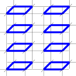
Figure 6: The 3D dimerized plaquette quantum antiferromagnetic Heisenberg model studied in this investigation Tan20.2 .

— The 3D 5-state ferromagnetic Potts model Tan20.1 —

The Hamiltonian $H_{\text{Potts}}$ of the 5-state Potts model on the 3D cubic lattice considered in our study is given by Wu82 ; Swe87 ; Wan89 ; Wan90

$$\beta H_{\text{Potts}}=-J\beta\sum_{\left<ij\right>}\delta_{\sigma_{i},\sigma_{j}},$$ (8)

where $J>0$, $\beta$ is the inverse temperature and similar to the convention introduced earlier, here $\left<ij\right>$ stands for the nearest neighbor sites $i$ and $j$. In addition, in Eq. (8) the $\delta$ refers to the Kronecker function and finally, the Potts variable $\sigma_{i}$ appearing above at each site $i$ takes an integer value from $\{1,2,3,4,5\}$.

The observables considered here for the 3D 5-state ferromagnetic Potts model are again the first and the second Binder ratios ($Q_{1}$ and $Q_{2}$) which are expressed as

$$Q_{1} = \langle|m|\rangle^{2}/\langle m^{2}\rangle,$$ (9)

$$Q_{2} = \langle m^{2}\rangle^{2}/\langle m^{4}\rangle,$$ (10)

where on a cubic lattice with a linear box size $L$ the $m$ appearing above is defined as

$$m=\frac{1}{L^{3}}\sum_{j}\exp\left(i\frac{2\pi\sigma_{j}}{5}\right),$$ (11)

and the summation is over all sites.

As the temperature $T$ changes from low to high, phase transitions will take place for the 3D classical $O(3)$ and the 5-state ferromagnetic Potts models. The critical points $T_{c}$ of the 3D classical $O(3)$ and the 5-state ferromagnetic Potts models as well as the $g_{c}$ of the 3D plaquette model described above have been calculated with high accuracy in the literature Hol92 ; Cam02 ; Has05 ; San10 ; Tan18 .

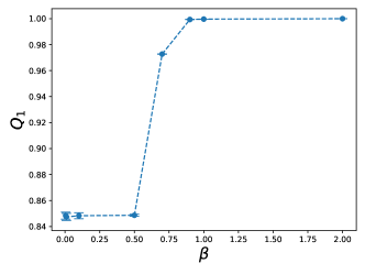
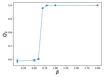
Figure 7: $Q_{1}$ (top panel, obtained on $12^{3}$ lattices) and $Q_{2}$ (bottom panel, obtained on $48^{3}$ lattices) as functions of $\beta$ for the 3D classical $O(3)$ model.

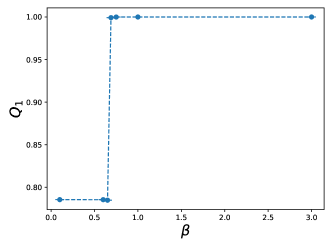
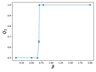
Figure 8: $Q_{1}$ (top panel, obtained on $20^{3}$ lattices) and $Q_{2}$ (bottom panel, obtained on $20^{3}$ lattices) as functions of $\beta$ for the 3D 5-state ferromagnetic Potts model.

The construction of the configurations used for the NN testing — As pointed out in the main text, bulk quantities satisfying certain conditions are suitable for employing to construct the configurations used for the NN testing. For all the three considered models, we find that the first and the second Binder ratios ($Q_{1}$ and $Q_{2}$) are the appropriate observables that suit these criterions. Indeed, as can be see in figs. 7, 8, and 9, $Q_{1}$ and $Q_{2}$ of the three studied systems fulfill the requirements outlined previously.

We would like to emphasize the fact that when choosing the relevant quantities, like the Binder ratios $Q_{1}$ and $Q_{2}$, only several data points are sufficient to determine whether the targeted observables meet the required criterion.

The second method of constructing the configurations for the NN prediction are already detailed in Ref. Tan20.2 . Here we will use the $O(3)$ model to show how to convert the associated spin states into the suitable variables used for the testing.

For a given $O(3)$ configuration, the associated 1D lattice of 120 sites is built as follows. First, 120 sites of the given $O(3)$ configuration is chosen randomly and uniformly. Second, $\psi\,\,\text{mod}\,\,\pi$ for these 120 chosen sites from the given $O(3)$ configuration, which is ether 1 or 0, are used as the variables for the 120 sites 1D lattice.

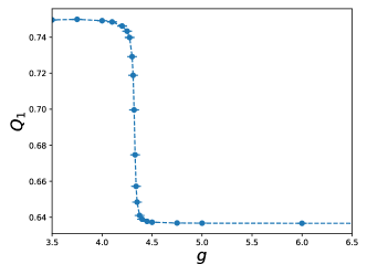
Figure 9: $Q_{1}$ as a function of $g$ for the 3D plaquette model. The results are obtained on $32^{3}$ cubic lattices.

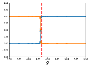
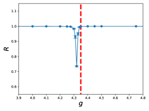
Figure 10: Individual component (top) and magnitude $R$ (bottom) of the output vectors as functions of $\beta$ for the 3D plaquette model. The results are obtained by the NN trained on a 2D square lattice with linear size $L=16$, and the configurations employed for the prediction are based on $Q_{2}$ (on $32^{3}$ lattices) of the considered model. The vertical dashed line in both panel is the expected (lower bound of) $g_{c}$.

More NN results — In the main text, the NN trained on a 1D lattice of 120 sites is used and here we present more outcomes obtained using this NN. Moreover, we also train two NNs on a 1D lattice of 200 sites and on a 16 by 16 square lattice. The corresponding results will be demonstrated as well. These additional results again confirm the effectiveness of our extremely efficient NN approach for investigating the critical phenomena.

Fig. 9 shows the quantity $Q_{1}$ of the 3D plaquette model. The results in the figure indicate the associated critical point $g_{c}$ is between $g=4.0$ and $g=4.5$. In addition, the outcomes of the NN (trained on a 16 by 16 square lattice) using the crossing and the magnitude methods are demonstrated as the top and the bottom panels of fig. 10. The dashed vertical line in both panels is the lower bound of $g_{c}$ estimated using the relevant data. Clearly, the agreement between the NN and the expected results is remarkable.

Fig. 11 shows the crossing associated with the 3D classical $O(3)$ model. The outcomes are obtained using a NN trained on a 1D lattice of 120 sites and the configurations employed for the prediction are based on the bulk quantity $Q_{1}$ of the studied model. Moreover, the $Q_{1}$ for calculating the outcomes of the top and the bottom panels are determined on lattices with linear system sizes $L=12$ and $L=48$, respectively. As can been seen from the figure, the crossing points move toward the expected $\beta_{c}$ as the linear system size $L$ increases.

The results using configurations based on the detailed spin states of the $O(3)$ model for the prediction are shown in fig. 12. The demonstrated results are obtained with NN trained on a 1D lattice of 200 sites.

Similarly, same scenario is observed for the 3D 5-state Potts model, see fig. 13. It is interesting that although the targeted phase transition associated with the 3D 5-state Potts model is first order, the trained NN is capable of estimating the corresponding $\beta_{c}$ with high accuracy.

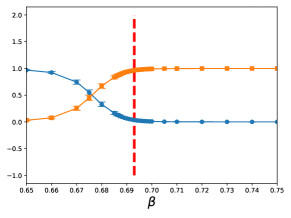
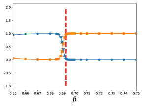
Figure 11: Individual component of the output vectors as functions of $\beta$ for the 3D classical $O(3)$ model. The dashed line is the expected $\beta_{c}$. The results are obtained by the NN trained on a 1D lattice of 120 sites, and the configurations employed for the prediction are based on $Q_{1}$ of the considered model.

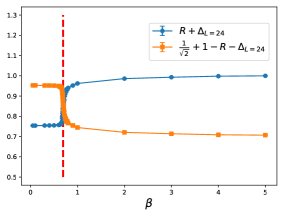
Figure 12: $R+\Delta$ and $1/\sqrt{2}+1-R-\Delta$ as functions of $\beta$ for the 3D classical $O(3)$ model. The dashed line is the expected $\beta_{c}$. The results are obtained by the NN trained on a 1D lattice of 200 sites, and the configurations employed for the prediction are based on the microscopic spin states of the considered model.

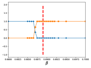
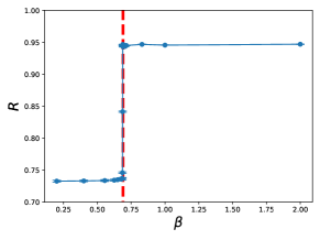
Figure 13: (Top panel) Individual component of the output vectors as functions of $\beta$ for the 3D 5-state ferromagnetic Potts model. The results are obtained by the NN trained on a 1D lattice of 120 sites. The configurations employed for the prediction are based on $Q_{1}$ (on $20^{3}$ lattices) of the considered model. (Bottom panel) The magnitude $R$ of the NN outputs as a function of $\beta$ for the 3D 5-state ferromagnetic Potts model. The results are obtained by the NN trained on a 1D lattice of 200 sites. The configurations employed for the prediction are based on the detailed Potts configurations (on $20^{3}$ lattices) of the considered model.

Comments and Remarks —

In this final part of the supplemental materials, several remarks (comments) regarding the NN methods proposed in the main text are listed.

1. The only requirement needed in our approach is the availability of bulk observables satisfying certain conditions mentioned explicitly in the main text. It is obvious that such requirements are met in almost all the studies (both theory and experiment) associated with phase transitions.

2. The approach demonstrated here does not depend on the microscopic details of considered models. Therefore, it is anticipated that our method is applicable for (any) other systems when phase transitions are concerned.

3. Crossings may take place at high temperatures other than the targeted critical points. With the idea of using appropriate bulk quantities as input for the NN calculations, these situations have no influence on our high precision determination of the studied phase transitions.

4. In our NN calculations, only the kernel $L_{2}$ regularization (with the argument being set to 1) is considered. Such a strategy works well for all the studied models.

5. Although further investigation is required, for the quantum plaquette model, using microscopic spin states to produce configurations for the prediction does not seem to work.

6. For the 3D 5-state ferromagnetic Potts model, the second method of constructing 1D configurations of 120 sites for the NN prediction proceeds as follows. First, 120 sites of a given Potts configurations are chosen one by one (randomly and uniformly). Second, whenever the Potts variable of the picked site is 1 or 3 (2 or 4), the associated 1D lattice position is assigned the integer 0 (1). If the Potts variable is 5, then 1 and 0 are given to the corresponding (1D lattice) site with equal probability.

7. We have carried out a NN calculation to determine the $T_{c}$ of the 3D $O(3)$ model using the standard procedure. In particular, 4 temperatures are chosen (two are below and two are above $T_{c}$) and the corresponding (totally 4000) spin state configurations on $48^{3}$ lattices are used for the training. The time taken to complete such a standard training step is around 400 times the time required for the NN training (on a 200 sites 1D lattice) conducted in this study.

References

- (1) Matthias Rupp, Alexandre Tkatchenko, Klaus-Robert Müller, and O. Anatole von Lilienfeld, Fast and Accurate Modeling of Molecular Atomization Energies with Machine Learning, Phys. Rev. Lett. 108 058301 (2012).
- (2) John C. Snyder, Matthias Rupp, Katja Hansen, Klaus-Robert Müller, and Kieron Burke, Finding Density Functionals with Machine Learning, Phys. Rev. Lett. 108 253002 (2012).
- (3) Zhenwei Li, James R. Kermode, and Alessandro De Vita, Molecular Dynamics with On-the-Fly Machine Learning of Quantum-Mechanical Forces, Phys. Rev. Lett. 114, 096405 (2015).
- (4) P. Baldi, P. Sadowski and D. Whiteson, Enhanced Higgs Boson to Search with Deep Learning, Phys. Rev. Lett. 114, 111801 (2015).
- (5) V. Mnih, K. Kavukcuoglu, D. Silver, A. A. Rusu, J. Veness, M. G. Bellemare, A. Graves, M. Riedmiller, A. K. Fidjeland, G. Ostrovski, S. Petersen, C. Beattie, A. Sadik, I. Antonoglou, H. King, D. Kumaran, D. Wierstra, S. Legg and D. Hassabis, Human-level control through deep reinforcement learning, Nature 518, no.7540, 529-533 (2015).
- (6) J. Searcy, L. Huang, M. A. Pleier and J. Zhu, Determination of the polarization fractions in using a deep machine learning technique, Phys. Rev. D 93, no.9, 094033 (2016).
- (7) P. Baldi, K. Cranmer, T. Faucett, P. Sadowski and D. Whiteson, Parameterized neural networks for high-energy physics, Eur. Phys. J. C 76, no.5, 235 (2016).
- (8) P. Baldi, K. Bauer, C. Eng, P. Sadowski and D. Whiteson, Jet Substructure Classification in High-Energy Physics with Deep Neural Networks, Phys. Rev. D 93, 094034 (2016).
- (9) Giacomo Torlai and Roger G. Melko, Learning thermodynamics with Boltzmann machines, Phys. Rev. B 94, 165134 (2016).
- (10) Lei Wang, Discovering phase transitions with unsupervised learning , Phys. Rev. B 94, 195105 (2016).
- (11) M. Attarian Shandiz and R. Gauvin Application of machine learning methods for the prediction of crystal system of cathode materials in lithium-ion batteries, Computational Materials Science 117 (2016) 270-278.
- (12) Tomoki Ohtsuki and Tomi Ohtsuki, Deep Learning the Quantum Phase Transitions in Random Two-Dimensional Electron Systems, J. Phys. Soc. Jpn. 85, 123706 (2016).
- (13) B. Hoyle, Measuring photometric redshifts using galaxy images and Deep Neural Networks, Astron. Comput. 16, 34-40 (2016).
- (14) Juan Carrasquilla, Roger G. Melko, Machine learning phases of matter, Nature Physics 13, 431–434 (2017).
- (15) Giuseppe Carleo, Matthias Troyer, Solving the quantum many-body problem with artificial neural networks, Science 355, 602 (2017).
- (16) Peter Broecker, Juan Carrasquilla, Roger G. Melko, and Simon Trebst, Machine learning quantum phases of matter beyond the fermion sign problem, Scientific Reports 7, 8823 (2017).
- (17) Kelvin Ch’ng, Juan Carrasquilla, Roger G. Melko, and Ehsan Khatami, Machine Learning Phases of Strongly Correlated Fermions, Phys. Rev. X 7, 031038 (2017).
- (18) Akinori Tanaka, Akio Tomiya, Detection of Phase Transition via Convolutional Neural Networks, J. Phys. Soc. Jpn. 86, 063001 (2017).
- (19) Evert P.L. van Nieuwenburg, Ye-Hua Liu, Sebastian D. Huber, Learning phase transitions by confusion, Nature Physics 13, 435–439 (2017).
- (20) A. Mott, J. Job, J. R. Vlimant, D. Lidar and M. Spiropulu, Solving a Higgs optimization problem with quantum annealing for machine learning, Nature 550, no.7676, 375-379 (2017).
- (21) Junwei Liu, Huitao Shen, Yang Qi, Zi Yang Meng, Liang Fu, Self-learning Monte Carlo method and cumulative update in fermion systems, Phys. Rev. B 95, 241104(R) (2017).
- (22) Tomoyuki Tamura et al, Fast and scalable prediction of local energy at grain boundaries: machine-learning based modeling of first-principles calculations, (2017) Modelling Simul. Mater. Sci. Eng. 25 075003.
- (23) J. Tubiana and R. Monasson, Emergence of Compositional Representations in Restricted Boltzmann Machines, Phys. Rev. Lett. 118, 138301 (2017).
- (24) Xiao Yan Xu, Yang Qi, Junwei Liu, Liang Fu, Zi Yang Meng, Self-learning quantum Monte Carlo method in interacting fermion systems, Phys. Rev. B 96, 041119(R) (2017).
- (25) Li Huang and Lei Wang, Phys. Rev. B 95, 035105 (2017).
- (26) Junwei Liu, Yang Qi, Zi Yang Meng, Liang Fu, Self-learning Monte Carlo method, Phys. Rev. B 95, 041101(R) (2017).
- (27) Yuki Nagai, Huitao Shen, Yang Qi, Junwei Liu, and Liang Fu Phys. Rev. B 96 161102 (2017).
- (28) Kolb, B., Lentz, L. C. and Kolpak, A. M., Discovering charge density functionals and structure-property relationships with PROPhet: A general framework for coupling machine learning and first-principles methods, Sci Rep 7, 1192 (2017).
- (29) Dong-Ling Deng, Xiaopeng Li, and S. Das Sarma, Machine learning topological states, Phys. Rev. B 96 195145 (2017).
- (30) Yi Zhang, Roger G. Melko, and Eun-Ah Kim Machine learning Z2 quantum spin liquids with quasiparticle statistics. Phys. Rev. B 96, 245119 (2017).
- (31) Yi Zhang and Eun-Ah Kim, Quantum Loop Topography for Machine Learning, Phys. Rev. Lett. 118, 216401 (2017)
- (32) Wenjian Hu, Rajiv R. P. Singh, and Richard T. Scalettar, Discovering phases, phase transitions, and crossovers through unsupervised machine learning: A critical examination, Phys. Rev. E 95, 062122 (2017).
- (33) C.-D. Li, D.-R. Tan, and F.-J. Jiang, Applications of neural networks to the studies of phase transitions of two-dimensional Potts models, Annals of Physics, 391 (2018) 312-331.
- (34) Kelvin Ch’ng, Nick Vazquez, and Ehsan Khatami, Unsupervised machine learning account of magnetic transitions in the Hubbard model, Phys. Rev. E 97, 013306 (2018).
- (35) Lu, S., Zhou, Q., Ouyang, Y. et al., Accelerated discovery of stable lead-free hybrid organic-inorganic perovskites via machine learning, Nat Commun 9, 3405 (2018).
- (36) Matthew J. S. Beach, Anna Golubeva, and Roger G. Melko, Machine learning vortices at the Kosterlitz-Thouless transition, Phys. Rev. B 97, 045207 (2018).
- (37) L. G. Pang, K. Zhou, N. Su, H. Petersen, H. Stöcker and X. N. Wang, An equation-of-state-meter of quantum chromodynamics transition from deep learning, Nature Commun. 9, no.1, 210 (2018).
- (38) Phiala E. Shanahan, Daniel Trewartha, and William Detmold, Machine learning action parameters in lattice quantum chromodynamics, Phys. Rev. D 97, 094506 (2018).
- (39) Keith T. Butler, Daniel W. Davies, Hugh Cartwright, Olexandr Isayev, and Aron Walsh, Machine learning for molecular and materials science, Nature 559, 547–555 (2018).
- (40) Albert P. Bartoḱ, James Kermode, Noam Bernstein, and Gab́or Csańyi, Machine Learning a General-Purpose Interatomic Potential for Silicon, Phys. Rev. X 8, 041048 (2018).
- (41) Pengfei Zhang, Huitao Shen, and Hui Zhai, Machine Learning Topological Invariants with Neural Networks, Phys. Rev. Lett. 120, 066401 (2018).
- (42) A. Butter, G. Kasieczka, T. Plehn and M. Russell, Deep-learned Top Tagging with a Lorentz Layer, SciPost Phys. 5, no.3, 028 (2018).
- (43) Jun Gao et al. Experimental Machine Learning of Quantum States, Phys. Rev. Lett. 120, 240501 (2018).
- (44) Wanzhou Zhang, Jiayu Liu, and Tzu-Chieh Wei, Machine learning of phase transitions in the percolation and XY models, Phys. Rev. E 99, 032142 (2019).
- (45) Jonas Greitemann, Ke Liu, and Lode Pollet, Probing hidden spin order with interpretable machine learning, Phys. Rev. B 99, 060404(R) (2019).
- (46) J. Ren, L. Wu, J. M. Yang and J. Zhao, Exploring supersymmetry with machine learning, Nucl. Phys. B 943, 114613 (2019).
- (47) Xiao-Yu Dong, Frank Pollmann, and Xue-Feng Zhang, Machine learning of quantum phase transitions, Phys. Rev. B 99, 121104(R) (2019).
- (48) M. Cavaglia, K. Staats and T. Gill, Finding the origin of noise transients in LIGO data with machine learning, Commun. Comput. Phys. 25, no.4, 963-987 (2019).
- (49) Daniel W. Davies, Keith T. Butler, and Aron Walsh, Data-Driven Discovery of Photoactive Quaternary Oxides Using First-Principles Machine Learning, Chem. Mater. 2019, 31, 18, 7221–7230.
- (50) G. P. Conangla, F. Ricci, M. T. Cuairan, A. W. Schell, N. Meyer and R. Quidant, Optimal Feedback Cooling of a Charged Levitated Nanoparticle with Adaptive Control, Phys. Rev. Lett. 122, 223602 (2019)
- (51) Limeng Li, Yang You, Shunbo Hu, Yada Shi, Guodong Zhao, Chen Chen, Yin Wang, Alessandro Stroppa and Wei Ren, Electronic transport of organic-inorganic hybrid perovskites from first-principles and machine learning, Appl. Phys. Lett. 114, 083102 (2019).
- (52) Wenqian Lian et al. Machine Learning Topological Phases with a Solid-State Quantum Simulator, Phys. Rev. Lett. 122, 210503 (2019).
- (53) Pankaj Mehta, Marin Bukov, Ching-Hao Wang, Alexandre G.R. Day, Clint Richardson, Charles K. Fisher, and David J. Schwab, A high-bias, low-variance introduction to Machine Learning for physicists, Phys. Rep. 810, (2019) 1-124.
- (54) Joaquin F. Rodriguez-Nieva and Mathias S. Scheurer, Identifying topological order through unsupervised machine learning, Nat. Phys. 15, 790–795 (2019).
- (55) Giuseppe Carleo, Ignacio Cirac, Kyle Cranmer, Laurent Daudet, Maria Schuld, Naftali Tishby, Leslie Vogt-Maranto, and Lenka Zdeborová, Machine learning and the physical sciences, Rev. Mod. Phys. 91, 045002 (2019).
- (56) Tomi Ohtsuki and Tomohiro Mano, Drawing Phase Diagrams of Random Quantum Systems by Deep Learning the Wave Functions, J. Phys. Soc. Jpn. 89, 022001 (2020).
- (57) A. J. Larkoski, I. Moult and B. Nachman, Jet Substructure at the Large Hadron Collider: A Review of Recent Advances in Theory and Machine Learning, Phys. Rept. 841, 1-63 (2020).
- (58) X. Han and S. A. Hartnoll, Deep Quantum Geometry of Matrices, Phys. Rev. X 10, 011069 (2020).
- (59) D.-R. Tan et al. A comprehensive neural networks study of the phase transitions of Potts model, 2020 New J. Phys. 22 063016.
- (60) D.-R. Tan and F.-J. Jiang, Machine learning phases and criticalities without using real data for training, Phys. Rev. B 102, 224434 (2020).
- (61) Japneet Singh, Vipul Arora, Vinay Gupta, and Mathias S. Scheurer, Generative models for sampling and phase transition indication in spin systems, arXiv:2006.11868.
- (62) A. Lidiak and Z. Gong, Unsupervised Machine Learning of Quantum Phase Transitions Using Diffusion Maps, Phys. Rev. Lett. 125, no.22, 225701 (2020).
- (63) J. Carrasquilla, Machine Learning for Quantum Matter, Adv. Phys. X 5, no.1, 1797528 (2020).
- (64) Anthony Yu-Tung Wang, Ryan J. Murdock, Steven K. Kauwe, Anton O. Oliynyk, Aleksander Gurlo, Jakoah Brgoch, Kristin A. Persson, and Taylor D. Sparks, Chem. Mater. 2020, 32, 12, 4954–4965.
- (65) Zhilong Song et. al., 2020 Chinese Phys. B 29 116103.
- (66) Y. Cao, S. E. Agbemava, A. V. Afanasjev, W. Nazarewicz and E. Olsen, Landscape of pear-shaped even-even nuclei, Phys. Rev. C 102, no.2, 024311 (2020). Siwar Chibani and Francois-Xavier Couderta, Machine learning approaches for the prediction of materials properties, APL Materials 8, 080701 (2020).
- (67) J. Amacker, W. Balunas, L. Beresford, D. Bortoletto, J. Frost, C. Issever, J. Liu, J. McKee, A. Micheli and S. Paredes Saenz, et al. Higgs self-coupling measurements using deep learning in the final state, JHEP 12, 115 (2020).
- (68) D. Bachtis, G. Aarts and B. Lucini, Extending machine learning classification capabilities with histogram reweighting, Phys. Rev. E 102, no.3, 033303 (2020).
- (69) G. Aad et al. [ATLAS], Dijet resonance search with weak supervision using TeV collisions in the ATLAS detector, Phys. Rev. Lett. 125, no.13, 131801 (2020).
- (70) S. V. Beentjes and A. Khamseh, Higher-order interactions in statistical physics and machine learning: A model-independent solution to the inverse problem at equilibrium, Phys. Rev. E 102, no.5, 053314 (2020).
- (71) R. Morgan et al. [DES], Constraints on the Physical Properties of GW190814 through Simulations Based on DECam Follow-up Observations by the Dark Energy Survey, Astrophys. J. 901, no.1, 83 (2020).
- (72) R. J. Shalloo, S. J. D. Dann, J. N. Gruse, C. I. D. Underwood, A. F. Antoine, C. Arran, M. Backhouse, C. D. Baird, M. D. Balcazar and N. Bourgeois, et al. Automation and control of laser wakefield accelerators using Bayesian optimization, Nature Commun. 11, no.1, 6355 (2020).
- (73) Y. Tomita, K. Shiina, Y. Okabe and H. K. Lee, Machine-learning study using improved correlation configuration and application to quantum Monte Carlo simulation, Phys. Rev. E 102, no.2, 021302 (2020).
- (74) M. Cabero, A. Mahabal and J. McIver, GWSkyNet: a real-time classifier for public gravitational-wave candidates, Astrophys. J. Lett. 904, no.1, L9 (2020).
- (75) R. M. Geilhufe and B. Olsthoorn, Identification of strongly interacting organic semimetals, Phys. Rev. B 102, no.20, 205134 (2020).
- (76) R. Wang, Y. G. Ma, R. Wada, L. W. Chen, W. B. He, H. L. Liu and K. J. Sun, Nuclear liquid-gas phase transition with machine learning, Phys. Rev. Res. 2, no.4, 043202 (2020).
- (77) K. A. Nicoli, C. J. Anders, L. Funcke, T. Hartung, K. Jansen, P. Kessel, S. Nakajima and P. Stornati, Estimation of Thermodynamic Observables in Lattice Field Theories with Deep Generative Models, Phys. Rev. Lett. 126, no.3, 032001 (2021).
- (78) K. Binder, Finite size scaling analysis of Ising model block distribution functions, Z. Phys. B 43, 119 (1981).
- (79) F. Y. Wu, Rev. Mod. Phys. 54, 235 (1982).
- (80) R. H. Swendsen, and J.-S. Wang, (1987), Phys. Rev. Lett. 58(2), 86 (1987).
- (81) J.-S. Wang, R. H. Swendsen, and R. Kotecký, Phys. Rev. Lett. 63, 109 (1989).
- (82) Jian-Sheng Wang, Robert H. Swendsen, and Roman Kotecký, Phys. Rev. B 42, 2465 (1990).
- (83) Christian Holm and Wolfhard Janke, Finite-size scaling study of the three-dimensional classical Heisenberg model, Phys. Lett. A 173 (1993) 8.
- (84) Massimo Campostrini, Martin Hasenbusch, Andrea Pelissetto, Paolo Rossi, and Ettore Vicari, Critical exponents and equation of state of the three-dimensional Heisenberg universality class, Phys. Rev. B 65, 144520 (2002).
- (85) Martin Hasenbusch, The Two dimensional XY model at the transition temperature: A High precision Monte Carlo study, J. Phys. A 38 (2005) 5869-5884.
- (86) A. W. Sandvik, Computational Studies of Quantum Spin Systems, Lectures on the Physics of Strongly Correlated Systems XIV: Fourteenth Training Course in the Physics of Strongly Correlated Systems, edited by A. Avella and F. Mancini, AIP Conf. Proc. No. 1297 (AIP, New York, 2010), p. 135.
- (87) D.-R. Tan and F.-J. Jiang, Classification for the universal scaling of Néel temperature and staggered magnetization density of three-dimensional dimerized spin-1/2 antiferromagnets, Phys. Rev. B 97, 094405 (2018).
- (88) https://keras.io
- (89) https://www.tensorflow.org
- (90) U. Wolff, Collective Monte Carlo Updating for Spin Systems, Phys. Rev. Lett. 62, 361 (1989).
- (91) A. W. Sandvik, Stochastic series expansion method with operator-loop update, Phys. Rev. B 66, R14157 (1999).