A systematic association of subgraph counts over a network

Abstract

We associate all small subgraph counting problems with a systematic graph encoding/rep-resentation system which makes a coherent use of graphlet structures. The system can serve as a unified foundation for studying and connecting many important graph problems in theory and practice. We describe topological relations among graphlets (graph elements) in rigorous mathematics language and from the perspective of graph encoding. We uncover, characterize and utilize algebraic and numerical relations in graphlet counts/frequencies. We present a novel algorithm for efficiently counting small subgraphs as a practical product of our theoretical findings.

1 Introduction

Graph or network studies, classical or modern, inevitably examine subgraph structures and counts, especially small subgraphs. Detecting the presence or absence of a small subgraph $H$ in a larger graph $G$ under consideration is fundamental to several classical graph-theoretic problems such as graph recognition and graph classification [27, 12, 19, 9]. In the early 1930s, Whitney investigated graph connectivity with several small subgraph patterns [34], which in modern terms are triangles, claws, diamonds, and four-node cliques. Since then, if not earlier, the counts or distributions of small subgraphs with prescribed patterns have been persistently used as primitives to characterize, recognize and categorize graphs. We give in Section 5 a brief review of subgraph counting problems.

At the turn of the 21^st century, subgraph counts and distributions gained unprecedented attention and applications with the advent of real-world networks and the advance in network analysis techniques. Two seminal papers, among others, made a massive impact on applied network studies by using subgraph structures and counts. In 1998, Watts and Strogatz used triangles in their network centrality measure and network model [33]. In 2002, Milo and his five co-authors found and defined network motifs as simple network building blocks [26]. The seminal works inspired many new approaches in improtant applications such as in biochemistry for investigating gene interactions, in neurobiology for mapping neural pathways in the brain, in computer vision and graphics for image alignment. Frequently occurring subgraphs are used to analyze protein-protein interaction networks and metabolic networks for drug target discovery [10].

In fact, 2004 saw another important work by Pržulj, Corneil and Jurisica [30]. The authors introduced the concept and use of graphlets for network analysis, which extend the conventional approach with edges and triangles to small subgraphs of various topological structures and their statistical distributions. The work has gained more attention and appreciation over the years, mostly in the community of researchers investigating biological networks with statistical methods [31].

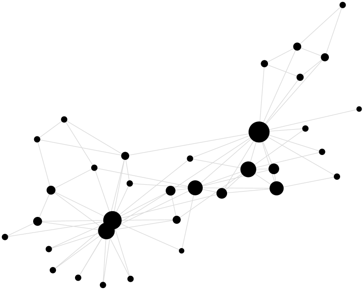
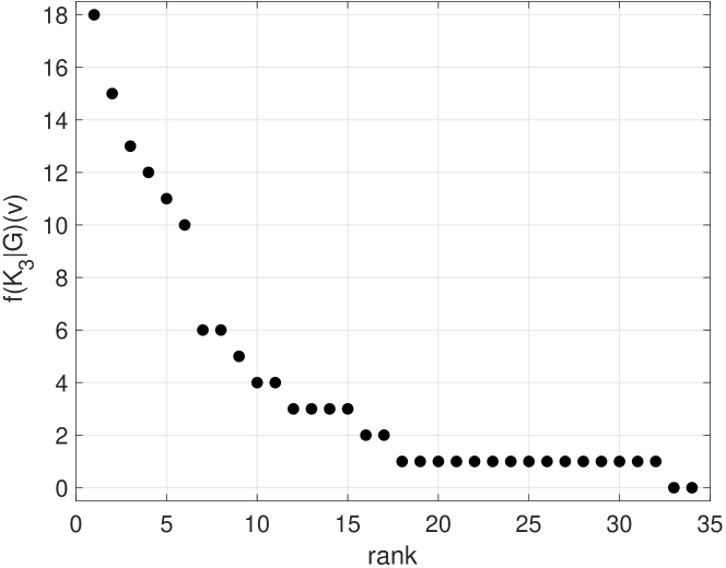
Figure 1: Triangle-frequency map (left) on Zachary’s karate club friendship network [36] and the triangle-frequency sequence (right). The network has $34$ club members and $78$ friendship links. The counts in the (spatial/topological) map have 1-1 association with club members (vertex labels), members in more triangle links are shown with larger markers. The counts in the (statistical) sequence are sorted in non-ascending order.

Applied network analysis and graph data mining with motifs or graphlet distributions remain ad hoc and in flux, by and large, with undiminished interest and enthusiasm yet lack of coherent understanding and principled decision making at multiple data analysis stages. This situation is reflected in multiple surveys and reviews [32, 20, 18, 1, 31, 7]. Rarely graphlet frequencies are connected to motif detection or discovery.

In the present work, we make a systematic association of all small subgraph counting problems with a graph encoding system which makes a coherent use of graphlet structures. The graph encoding/representation system can serve as a unified foundation for studying and connecting many significant graph problems in theory as well as in practice. In Section 2, we first give a formal description of multi-channel graph encoding with template graphs, in rigorous mathematics language and from the graph encoding perspective. We then focus on a system of graph encoding elements using what are known as graphlets. In Section 3, based on topological relations among the graphlets, we uncover, characterize, classify and utilize algebraic and quantitative relations in graphlet counts or frequencies. In Section 4, we present a novel algorithm for efficiently counting small subgraphs as a practical product of our theoretical findings. We show a significant reduction in the computation cost of generating graphlet maps on a real-world network. In Section 5, we comment on the connections made by our analysis among previous subgraph counting problems and methods. Certain shortcomings in some previous works become evident consequently. We also remark on potential applications of the present work.

2 Problem description & preliminary

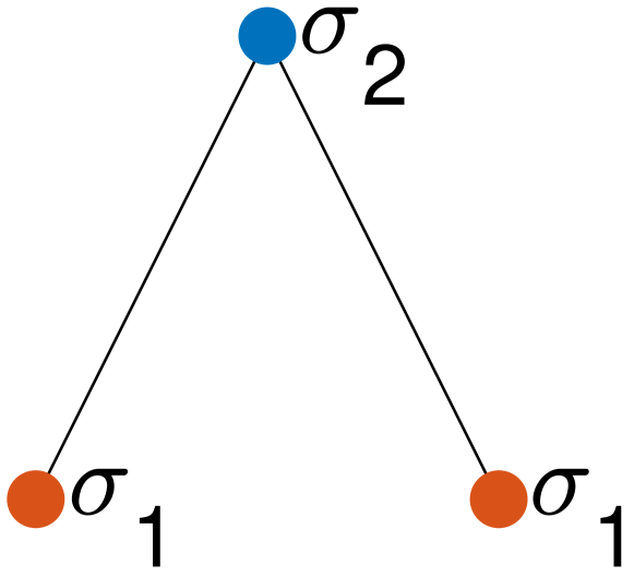
$H$

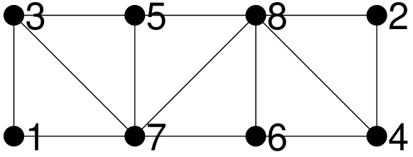
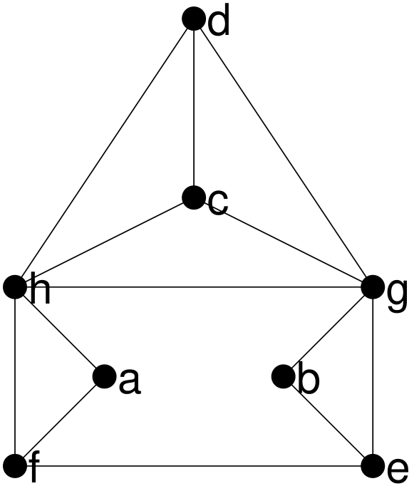
$G_{1}$

$G_{2}$

$v$	1	2	3	4	5	6	7	8
$d(v)$	2	2	3	3	3	3	5	5
$f(H|G)(v)$	4	4	4	4	7	7	9	9
$f({\color[rgb]{1,0,0}H_{\sigma_{1}}}|G)(v)$	4	4	3	3	6	6	3	3
$f({\color[rgb]{0,0.6470,0.9410}H_{\sigma_{2}}}|G)(v)$	0	0	1	1	1	1	6	6

$v$	a	b	c	d	e	f	g	h
$d(v)$	2	2	3	3	3	3	5	5
$f(H|G)(v)$	4	4	4	4	7	7	9	9
$f({\color[rgb]{1,0,0}H_{\sigma_{1}}}|G)(v)$	4	4	4	4	5	5	3	3
$f({\color[rgb]{0,0.6470,0.9410}H_{\sigma_{2}}}|G)(v)$	0	0	0	0	2	2	6	6

Figure 3: Graph differentiation by orbit-specific graphlet frequency sequences. The template graph $H$ is $K_{1,2}$, larger than $K_{2}$ and smaller than $K_{3}$. The leaf nodes of $H$ in red are in orbit $\sigma_{1}$, the root node in blue is in orbit $\sigma_{2}$. Graph $G_{1}$ and graph $G_{2}$ are attributed with their respective frequency sequence tables at the bottom. They have identical degree sequences, as shown in the first rows of the two tables. Their frequency sequences with respect to $H$ are also identical, as shown in the second rows of the tables. Graph $G_{1}$ and graph $G_{2}$ are differentiated by their orbit-specific vertex maps or sequences shown in the third and fourth rows, which decompose the sequences in the second rows.

We give a formal description of the basic subgraph counting problems. Any graph or network addressed in this paper is undirected, with simple edges and without self-loops. A graph is denoted by $G=G(V,E)$, with $V$ or $V(G)$ as the set of vertices or nodes and $E$ or $E(G)\subseteq V(G)\times V(G)$ as the set of edges or links. The primary sizes of graph $G$ are specified by $n=n(G)=|V(G)|$ and $m=m(G)=|E(G)|$. Graph $G^{\prime}$ is a subgraph of $G$ if $V(G^{\prime})\subseteq V(G)$ and $E(G^{\prime})\subseteq E(G)$. If $E(G^{\prime})=E(G)\cap(V(G)\times V(G))$ in addition, $G^{\prime}$ is an induced subgraph of $G$. A graph is connected if every pair of vertices is connected by a path. Two graphs $G_{1}$ and $G_{2}$ are isomorphic in topological link structure, $G_{1}\cong G_{2}$, if there is a bijection $\phi$ between $V(G_{1})$ and $V(G_{2})$ such that $(u,v)\in E(G_{1})$ implies $(\phi(u),\phi(v))\in E(G_{2})$ and vice versa. Graph $G$ is labeled if every vertex of $G$ has a unique label, or equivalently, the vertices are labeled from $1$ to $n(G)$. A graph to be characterized by its subgraph structures is referred to as a source graph.

2.1 One subgraph template: counts & maps

Definition 1.

(Subgraph counts over a source graph) Let $G$ be a labeled source graph. Let $H$ be a connected, unlabeled template graph, $n(H)\leq n(G)$. The gross count (or frequency) of $H$-isomorphic subgraphs in $G$ is $g(H|G)=|\Gamma_{g}(H|G)|$, where $\Gamma_{g}(H|G)=\mathopen{}\mathclose{{}\left\{H^{\prime}\subseteq G\mid H^{\prime}\cong H}\right\}$. Any two elements $H^{\prime},H^{\prime\prime}$ in $\Gamma_{g}(H|G)$ are two different subgraphs, $V(H^{\prime})\neq V(H^{\prime\prime})$. The net count is $f(H|G)=|\Gamma_{f}(H|G)|$, where $\Gamma_{f}(H|G)=\mathopen{}\mathclose{{}\left\{H^{\prime}\in\Gamma_{g}(H|G)\mid E(H^{\prime})=E(G)\cap(V(H^{\prime})\times V(H^{\prime}))}\right\}$.

The template size $n(H)$ is assumed bounded, throughout the rest of the paper, independent of any source graph. By Definition 1 the count of the induced subgraphs is more constrained, $f(H|G)\leq g(H|G)$. For any $K_{p}$, the clique with $p$ nodes, $p\geq 0$, $g(K_{p}|G)=f(K_{p}|G)$. In particular, $f(K_{2}|G)$ is the total number of edges in $G$, $m(G)=f(K_{2}|G)$. Two graphs with the same number of edges may be differentiated by their degree sequences. By extension, two networks with equal global counts with respect to (w.r.t.) the same template $H$, by Definition 1, may be differentiated by local counts at vertices.

Definition 2.

(Subgraph counts at incidence vertices) Let $G$ and $H$ be defined as in Definition 1. For every vertex $v$ in $V(G)$, let $\Gamma_{g}(H|G)(v)=\{H^{\prime}\in\Gamma_{g}(H|G)\mid v\in V(H^{\prime})\}$ and let $\Gamma_{f}(H|G)(v)=\{H^{\prime}\in\Gamma_{f}(H|G)\mid v\in V(H^{\prime})\}$. The gross count (or frequency) of $H$-isomorphic subgraphs incident with $v$ is $g(H|G)(v)=|\Gamma_{g}(H|G)(v)|$; the net count at $v$ is $f(H|G)(v)=|\Gamma_{f}(H|G)(v)|$.

In particular, $f(K_{2}|G)(v)$ is $d(v)$, the degree of $v$. The essence of Definition 2 is the introduction of a vertex map over $V(G)$ with respect to any particular template $H$. For instance, $f(K_{2}|G)(v)$ is a map onto vertex positions/locations/labels. The degree map gives rise to the degree sequence, which sorts the degrees in descending or ascending order with the vertex label or position information discarded. Similarly, $f(H|G)(v)$ gives rise to the frequency sequence of $G$ w.r.t. $H$, see the triangle-frequency map and triangle-frequency sequence in Figure 1.

The subgraph counts and maps defined above are graph invariants. They encode graph information.

2.2 Multi-channel graph encoding

The coding capacity for graph representation and differentiation can be increased by using multiple templates ${\cal H}=\{H_{p},\,p=1,2,\cdots,P\}$, $P>1$. For instance, in addition to the edge graph $K_{2}$ for encoding the degree information, one may also use $K_{1,2}$ of bi-fork pattern to encode more structural information. In Figure 3, two simple templates $K_{2}$ and $K_{1,2}$ are used to compare and differentiate graph $G_{1}$ and graph $G_{2}$.

Graph encoding with multiple templates has more discriminative capacity than with a single template. Let ${\cal H}$ be a collection of template graphs. Let $G$ be a source graph. By Definition 2, each template $H\in{\cal H}$ identifies with a unique net-frequency map (or heat map) over $V(G)$. There are multiple views at multiple granularity levels: local, regional and global. Locally at each vertex $v\in V(G)$, a unique $|{\cal H}|$-dimensional frequency (feature) vector $f({\cal H}|G)(v)$ is uniquely defined. The frequency vector at vertex $v$ encodes the topological structures in a neighborhood of the vertex; the frequency maps capture spatial and statistical information of pattern distributions and inter-pattern association or disassociation over the entire source graph or large regional subgraphs.

Besides the use of multiple template patterns, we describe the concept and approach of sub-channel decomposition for increasing code capacity without resorting to a new template pattern. For example, in [13] only two template patterns $K_{2}$ and $K_{1,2}$ are used to detect dynamic changes in temporal sequences of large, real-world networks. Three net-frequency maps are generated per network with greater discriminative power at about the same cost for generating two maps.

Sub-channel decomposition applies to any template graph $H$ with more than one orbits. The node set $V(H)$ can be uniquely partitioned into orbits, namely, disjoint subsets of equivalent nodes that are reflective, symmetric and transitive under automorphisms. An automorphism on $H$ is a link-invariant bijection $\phi$ on $V(H)$, i.e., $(u,v)\in E(H)$ if and only if $(\phi(u),\phi(v))\in E(H)$. When $H\cong H^{\prime}$, we denote by $\sigma\cong\sigma^{\prime}$ the correspondence between orbit $\sigma$ of $H$ and orbit $\sigma^{\prime}$ of $H^{\prime}$. In Figure 3, the template $K_{1,2}$ has two orbits, $\sigma_{1}$ and $\sigma_{2}$, which are color coded in red and blue, respectively.

Definition 3.

(Subgraph counts at orbit-specific incidence vertices.) Let $G$ and $H$ be defined as in Definition 1. Denote by $H_{\sigma}$ the template $H$ with orbit $\sigma$ designated for incidence. Let $\Gamma_{g}(H_{\sigma}|G)(v)=\{H^{\prime}_{\sigma^{\prime}}\in\Gamma_{g}(H|G)(v)\mid v\in\sigma^{\prime}\,\mbox{\rm and }\,\sigma^{\prime}\cong\sigma\}$. Let $\Gamma_{f}(H_{\sigma}|G)(v)=\{H^{\prime}_{\sigma^{\prime}}\in\Gamma_{f}(H|G)(v)\mid v\in\sigma^{\prime}\,\mbox{\rm and }\,\sigma^{\prime}\cong\sigma\}$. The gross count (or frequency) of $H$-isomorphic subgraphs with $\sigma$-specific incidence vertex at $v$ is $g(H_{\sigma}|G)(v)=|\Gamma_{g}(H_{\sigma}|G)(v)|$. The net count at $v$ is $f(H_{\sigma}|G)(v)=|\Gamma_{f}(H_{\sigma}|G)(v)|$.

We can precisely describe the sub-channel decomposition property as follows, $\forall v\!\in\!V(G)$,

$$\begin{array}[]{rc}f(H|G)(v)\!&\!=\displaystyle\sum_{\sigma\subset V(H)}f(H_{\sigma}|G)(v),\\ g(H|G)(v)\!&\!=\displaystyle\sum_{\sigma\subset V(H)}g(H_{\sigma}|G)(v).\end{array}$$ (1)

In Figure 3, graph $G_{1}$ and graph $G_{2}$ have identical degree sequences and identical $K_{1,2}$-frequency sequences. They are differentiated by the orbit-specific sequences w.r.t $K_{1,2}$.

Table 1: The size sequence of graphlet families ${\cal H}_{s}$ (graphlets with designated orbits) and the size sequence of families $\hat{\cal H}_{s}$ (graphlets without orbit partition), $1\leq s\leq 8$. Each sequence grows exponentially with $s$, the number of nodes in a family.

$s$	1	2	3	4	5	6	7	8
$|\mathcal{\hat{H}}_{s}|$	$1$	$1$	$2$	$6$	$21$	$112$	$853$	$11,117$
$|\mathcal{H}_{s}|$	$1$	$1$	$3$	$11$	$58$	$407$	$4306$	$72,489$

By utilizing the topological structure in a pattern template, the sub-channel encoding approach increases the discriminative power without or with little increase in the computation cost of subgraph counting. Assume the templates in ${\cal H}$ are made orbit-specific out of $P$ mutually non-isomorphic patterns, as in Definition 3. Denote by $a_{p}$ the number of orbits in a unique pattern $H_{p}$. Then, the code length of the frequency vector is $|{\cal H}|=\sum_{1\leq p\leq P}a_{p}$. The code length is greater than $P$. The difference is an indicator of the increased coding capacity for differentiating local structures. The first use of orbit-specific subgraph templates is seen in the original work of biological network analysis with graphlet degree distributions by Pržulj, Corneil and Jurisica in 2004 [30]. The above description by the present work elucidates, explains and characterizes the orbit-specific templates as sub-channel decomposition from the multi-channel encoding perspective.

By multi-channel graph encoding we refer to the use of multiple templates with optional use of the sub-channel decomposition approach. There are deeper potential and additional benefits with multi-channel graph coding. (a) The frequency features are derived, self-learned, from the source graph only. They can be joined with other attributes, or used to validate other features learned by different approaches. (b) The frequencies of a source graph are coupled by vertex collocation. This “spatial” collocation property increases the discriminative power. The frequency sequences are not independent of each other. Even when two different source graphs have identical sequences with respect to every template individually, their difference may be detected by comparing their vector-valued frequency sequences in lexicographical order. (c) The frequency vectors can be used to assess or detect self similarities within a source graph, among vertices or vertex subsets. (d) By using multiple connected templates, we have effectively included the case in which a template is composed of more than one connected components, especially for motif detection or discovery.

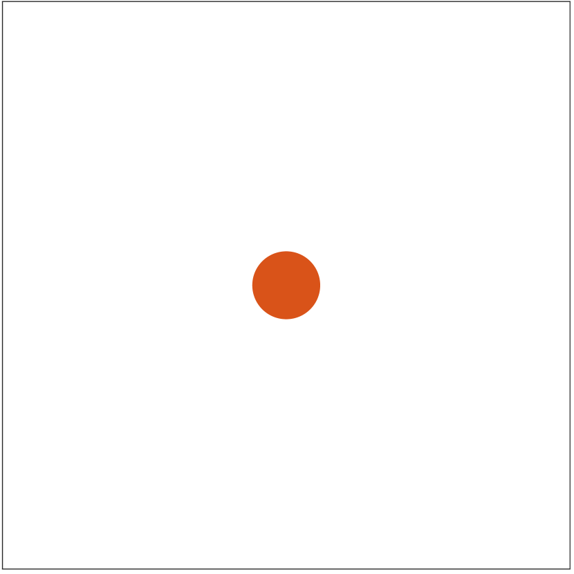
$H_{1,1,1}$

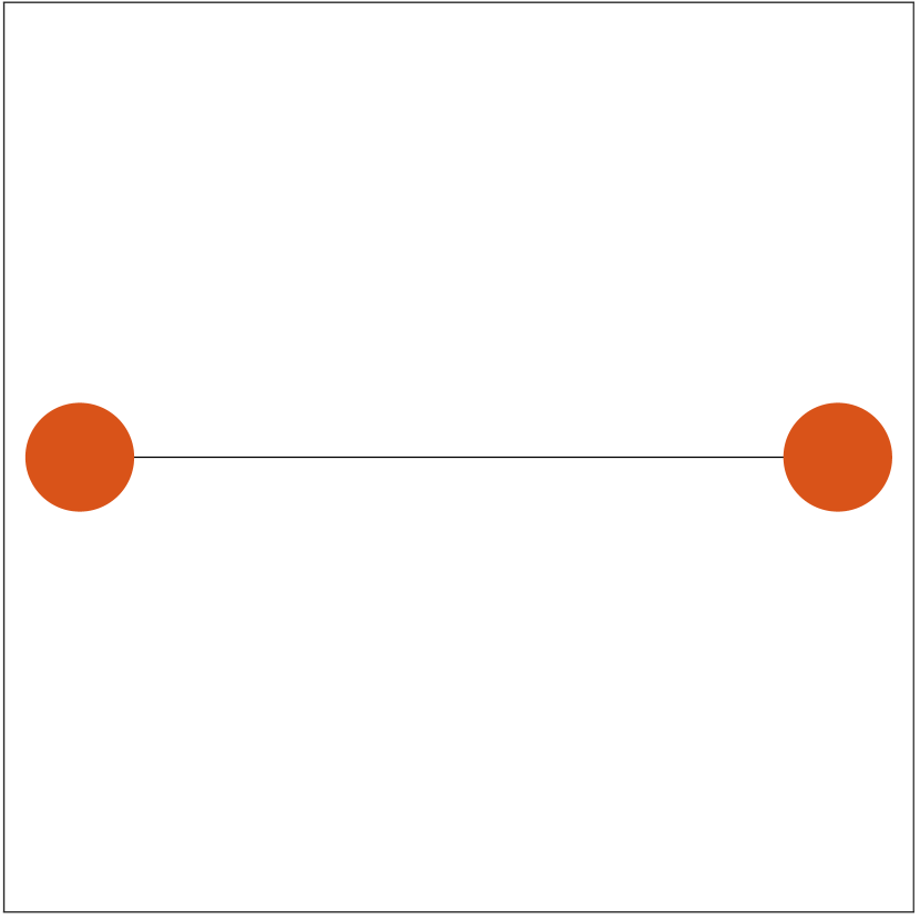
$H_{2,1,1}$

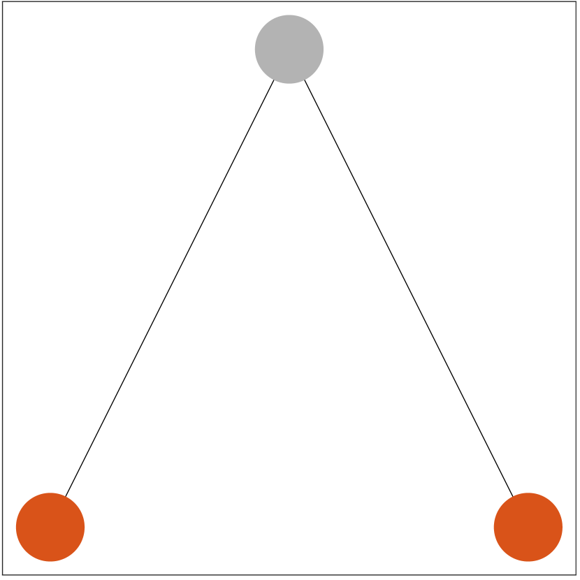
$H_{3,1,1}$

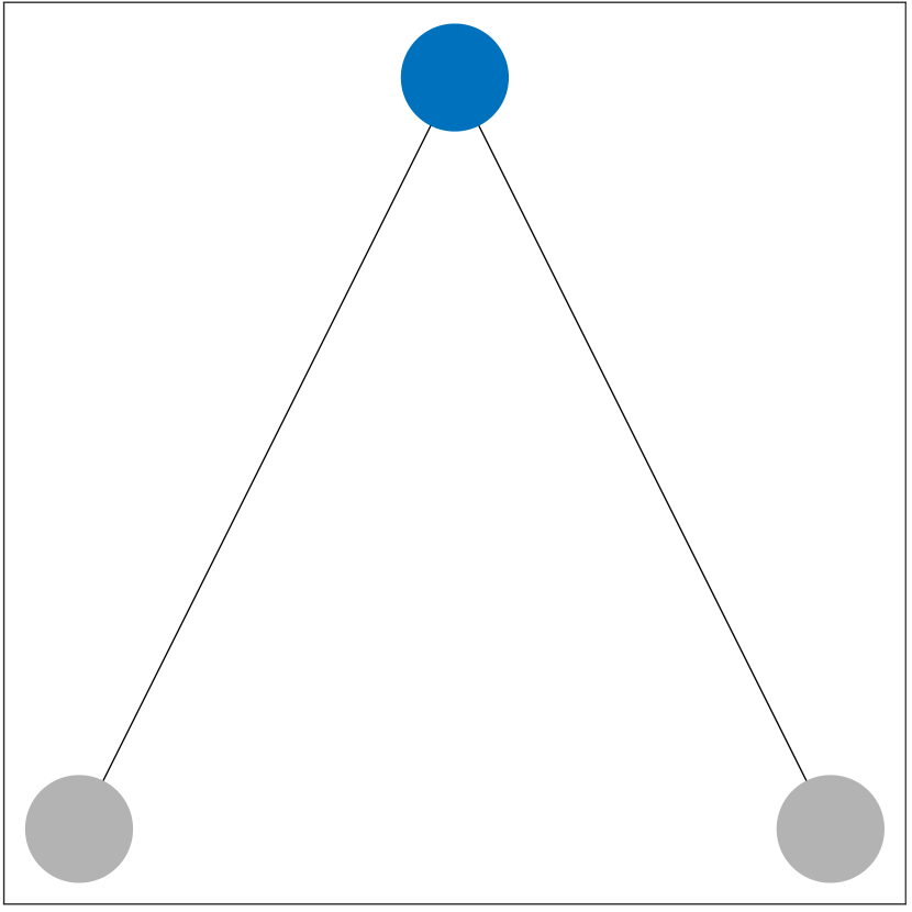
$H_{3,1,2}$

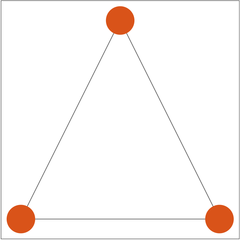
$H_{3,2,1}$

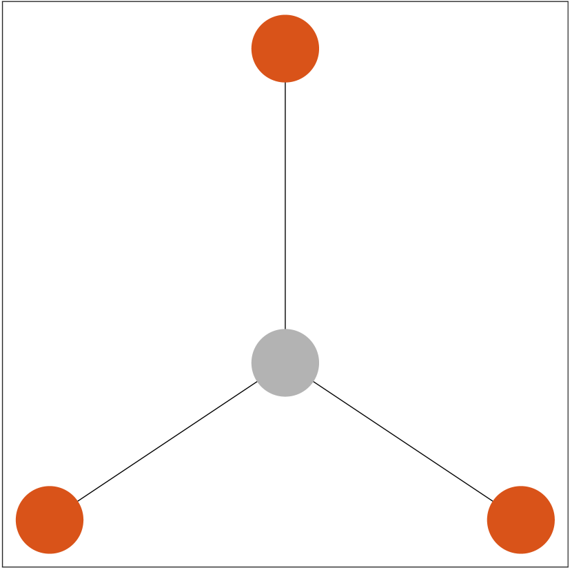
$H_{4,1,1}$

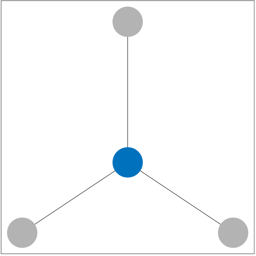
$H_{4,1,2}$

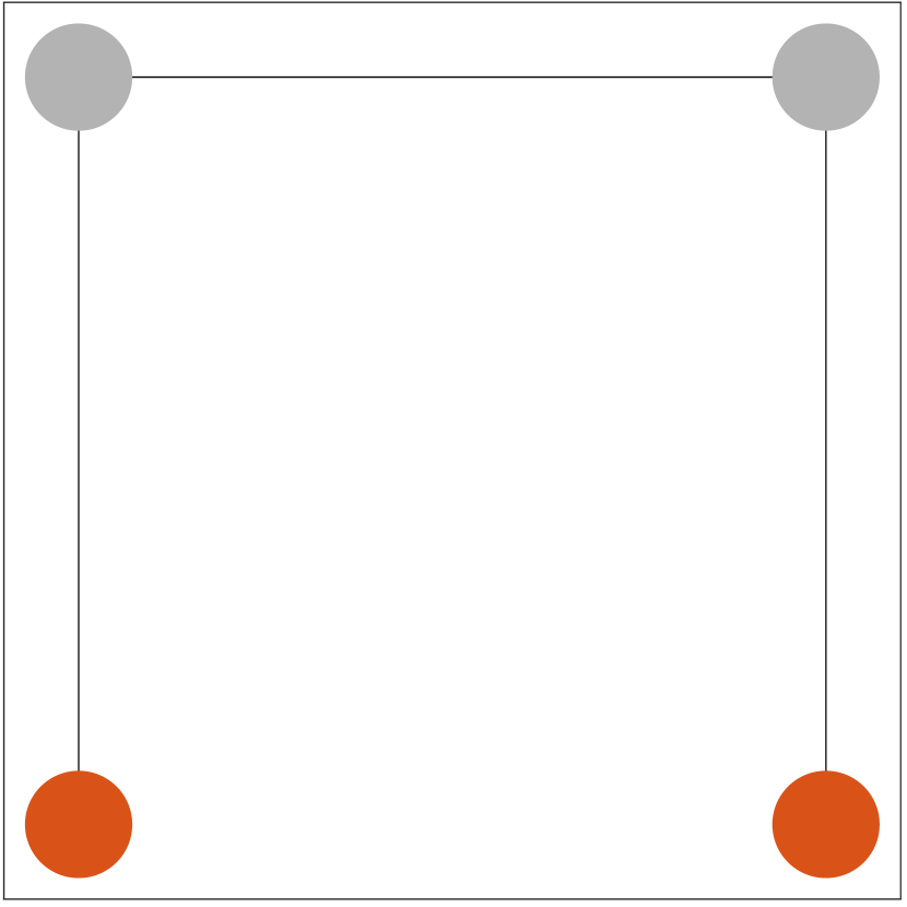
$H_{4,2,1}$

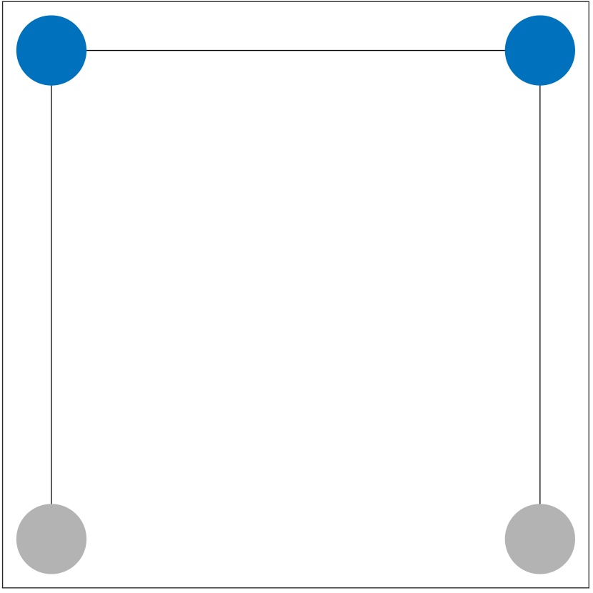
$H_{4,2,2}$

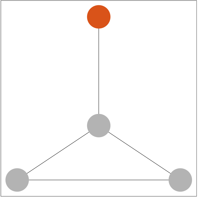
$H_{4,3,1}$

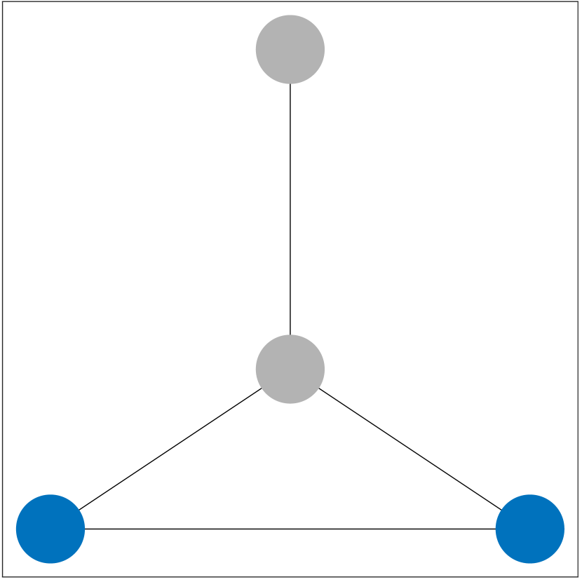
$H_{4,3,2}$

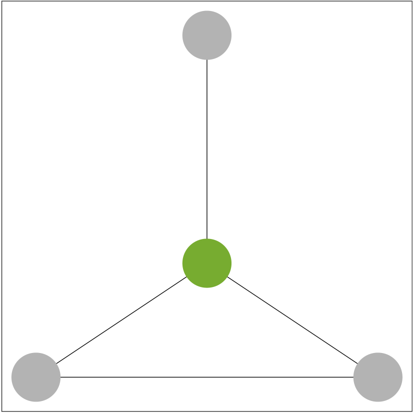
$H_{4,3,3}$

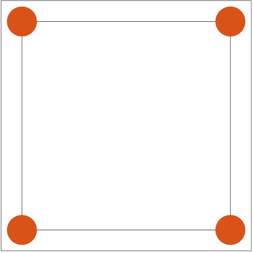
$H_{4,4,1}$

$H_{4,5,1}$

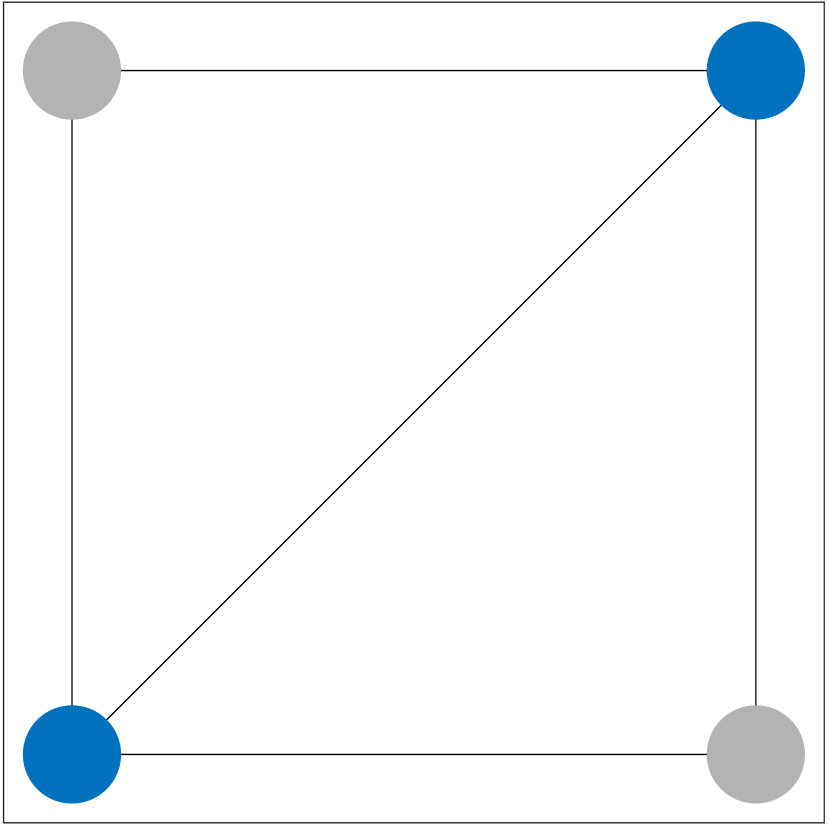
$H_{4,5,2}$

$H_{4,6,1}$

Figure 4: The dictionary of graphlets in the first four families ${\cal H}_{s}$, $s=1,2,3,4$. Each graphlet $H$ is identified by an index triplet $(s,p,\sigma)$, with $s=n(H)$, $p$ indexed to a unique topological pattern, and $\sigma$ to a specific orbit, as described in Section 2.3. Orbits indexed by $1$, $2$ and $3$ are color coded red, blue and green, respectively. The graphlets are placed from left to right, top to bottom, by the ordering scheme seira in Section 2.3.

2.3 Graphlet lattice neighborhoods

We focus on a system of multi-channel encoding graph elements known as graphlets. In this section, we give a clarified description of graphlets independent of source graphs and graphlet frequencies on any given source graph. More importantly, we introduce intrinsic topological relations among graphlets in the language of graph theory [11, 15] and lattice theory [6, 5]. These topological relationships are the foundation of the algebraic and quantitative relations in graphlet frequencies we further uncover and present in the rest of the paper.

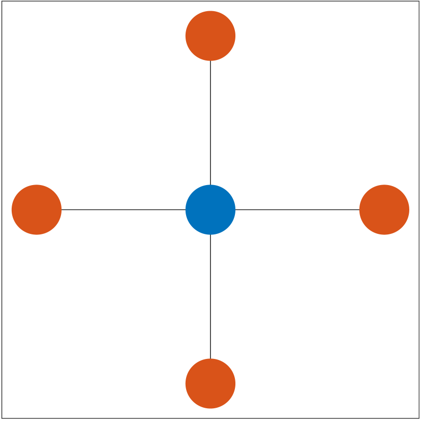
$H_{5,1}$

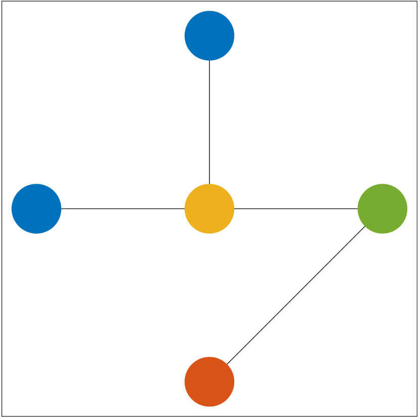
$H_{5,2}$

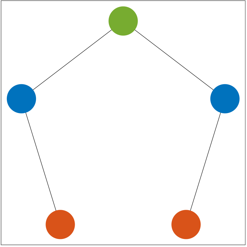
$H_{5,3}$

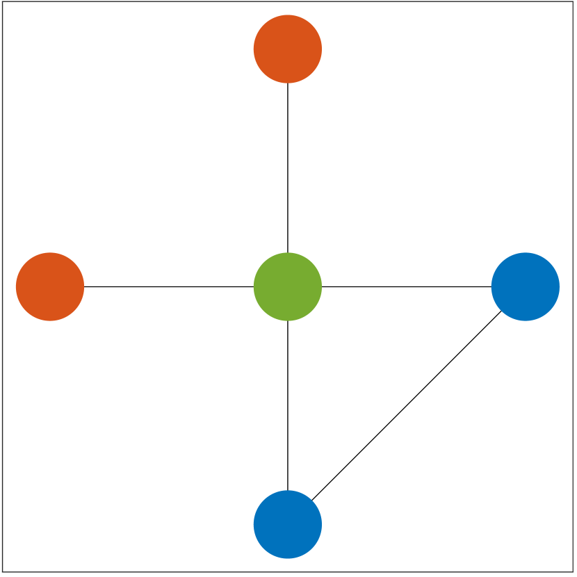
$H_{5,4}$

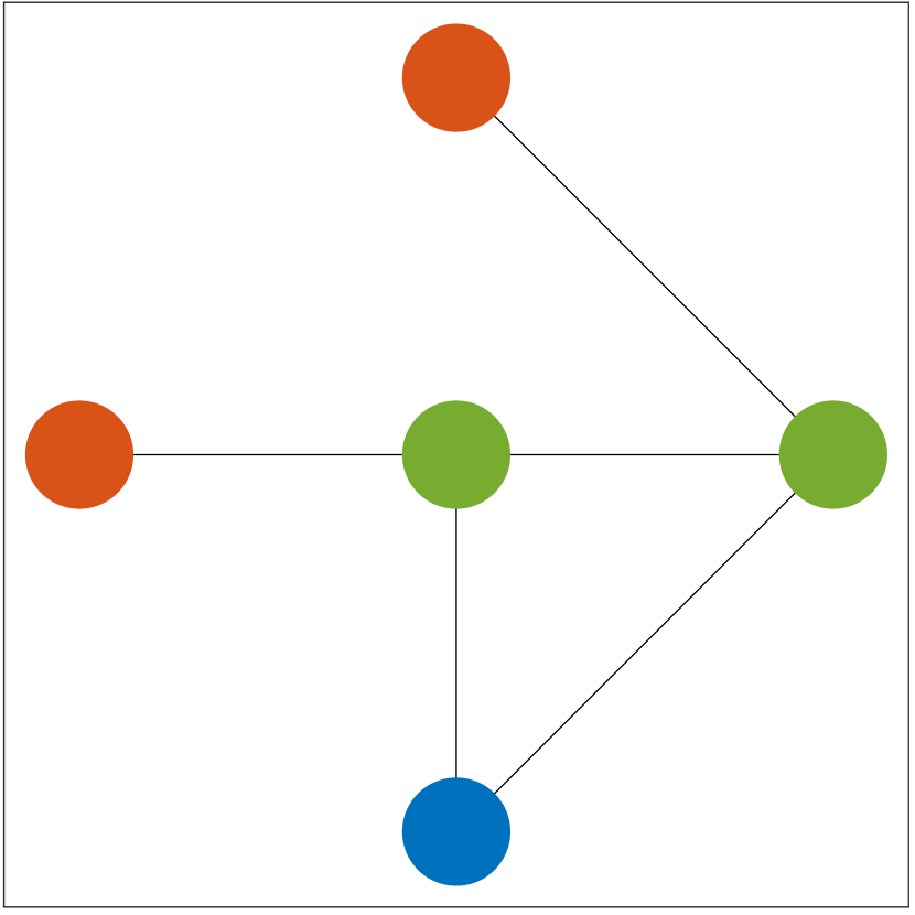
$H_{5,5}$

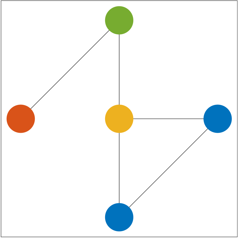
$H_{5,6}$

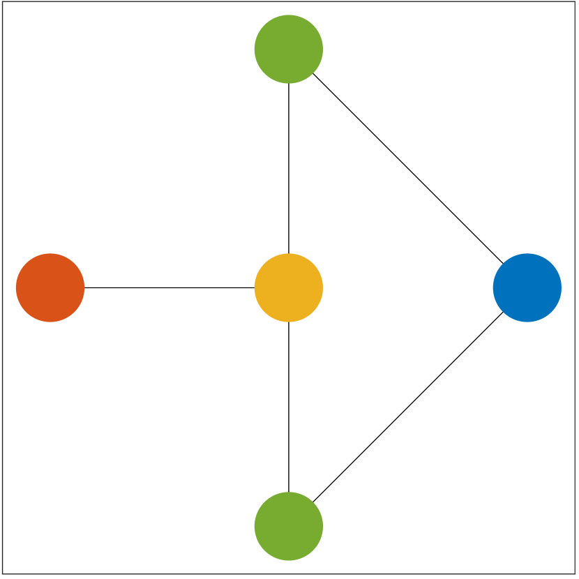
$H_{5,7}$

$H_{5,8}$

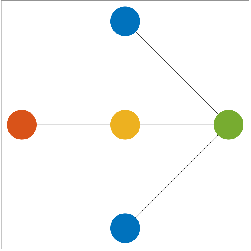
$H_{5,9}$

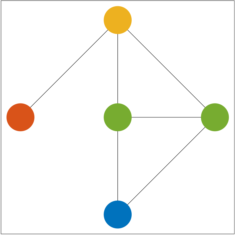
$H_{5,10}$

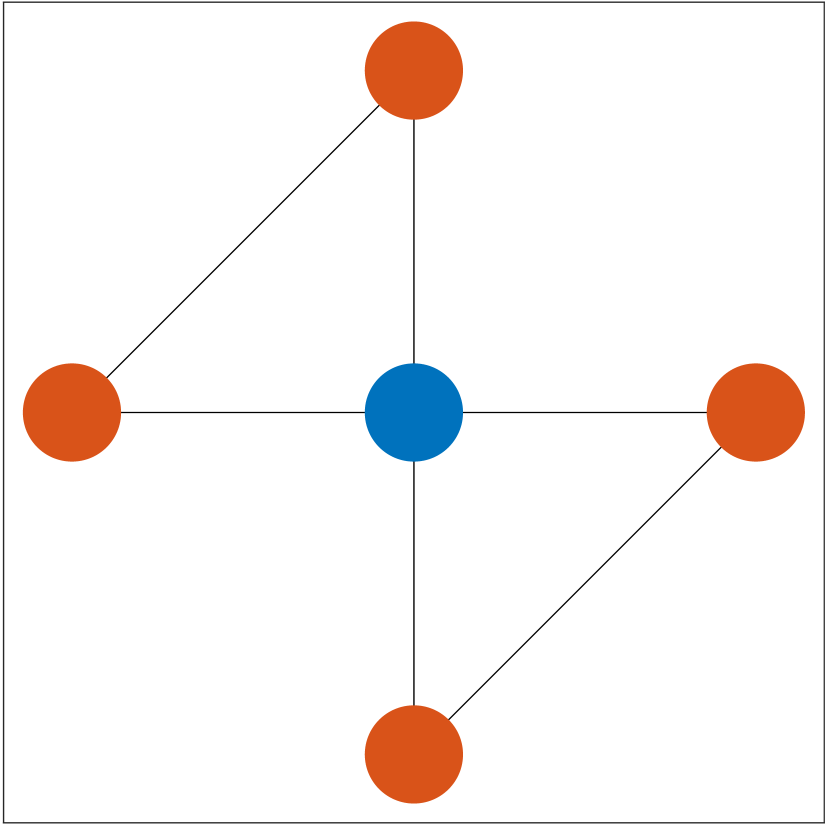
$H_{5,11}$

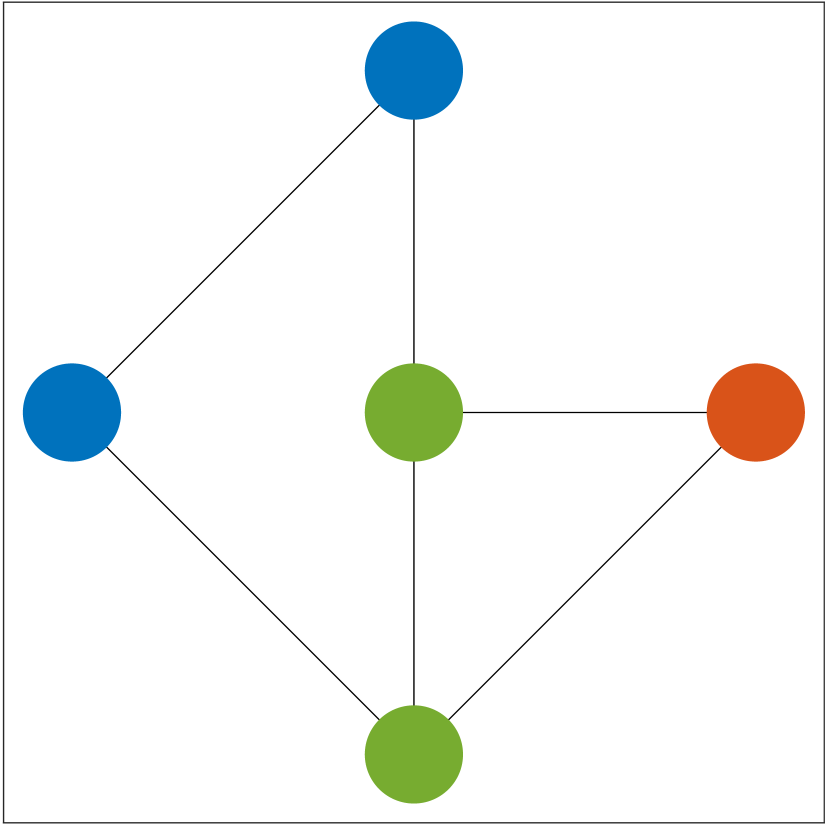
$H_{5,12}$

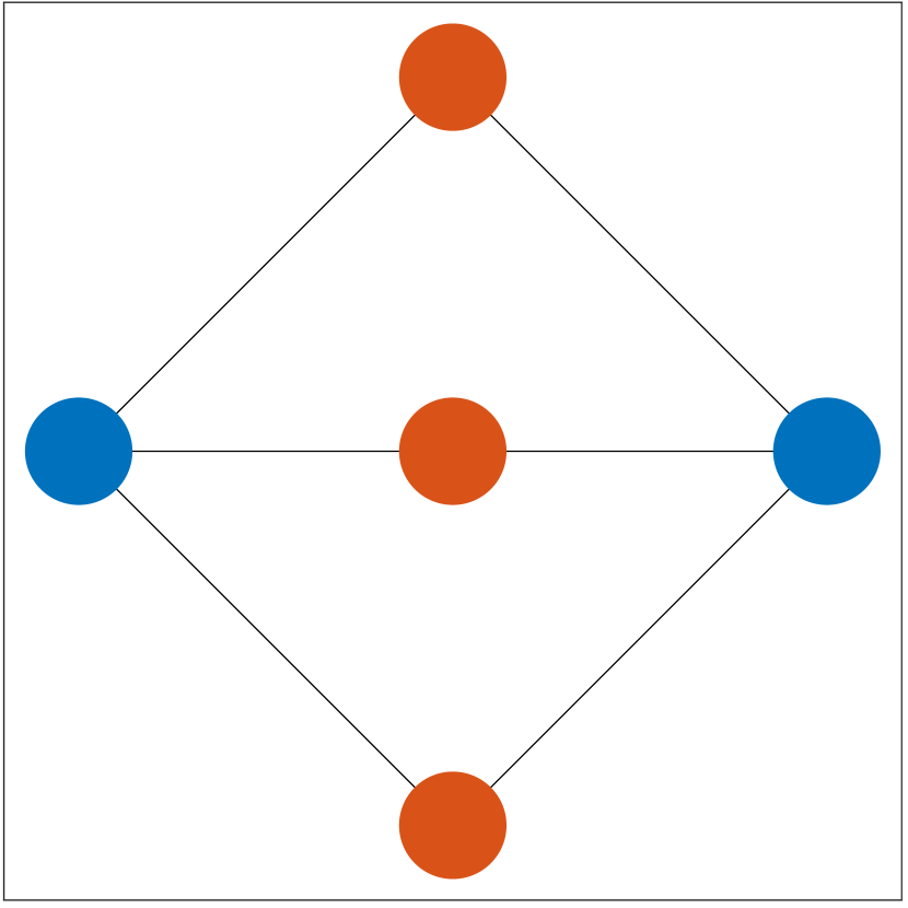
$H_{5,13}$

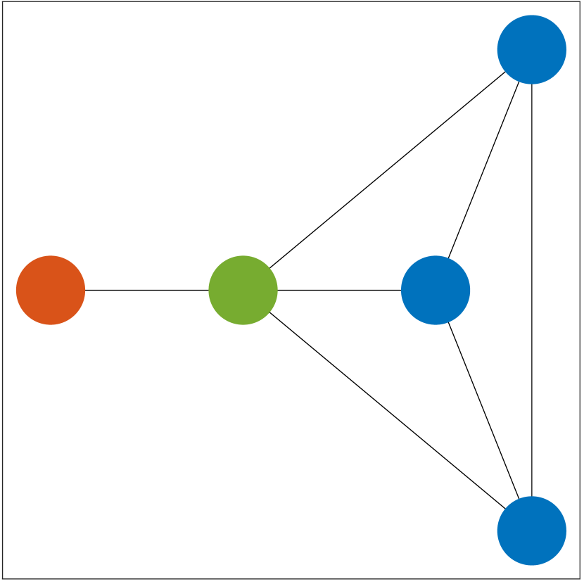
$H_{5,14}$

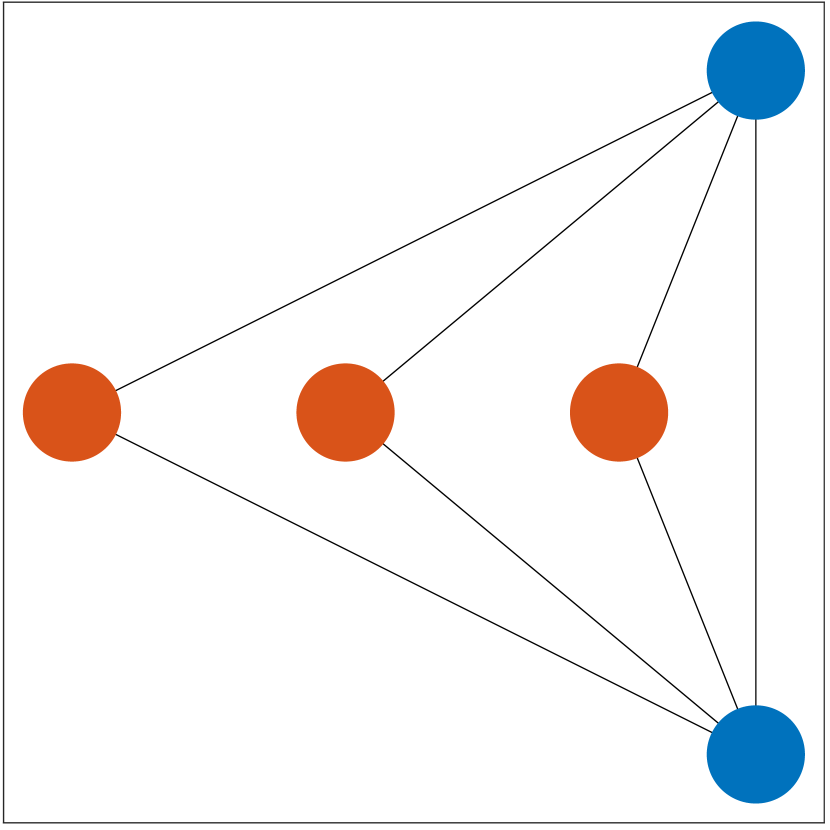
$H_{5,15}$

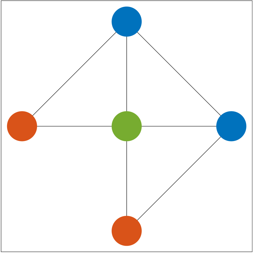
$H_{5,16}$

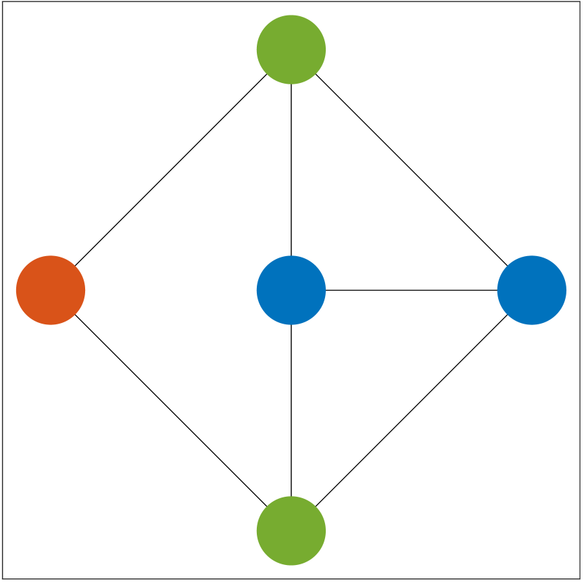
$H_{5,17}$

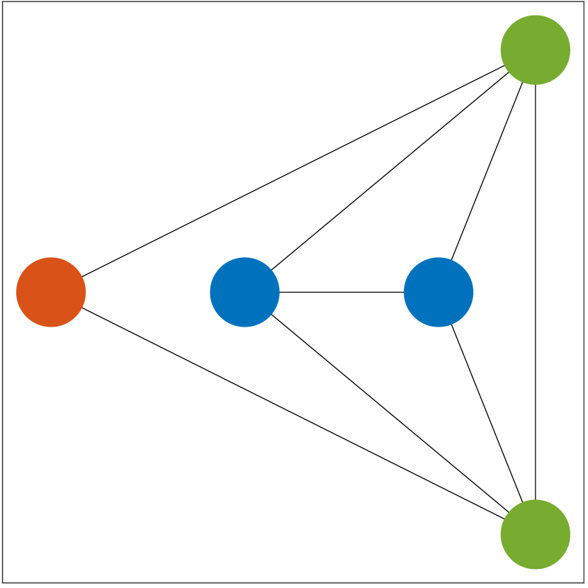
$H_{5,18}$

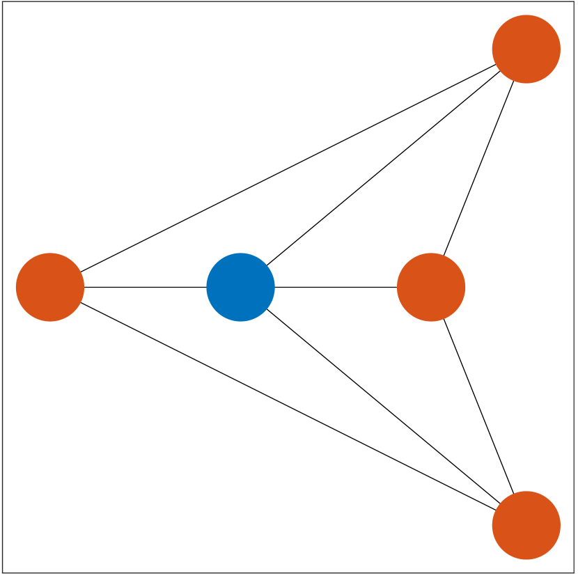
$H_{5,19}$

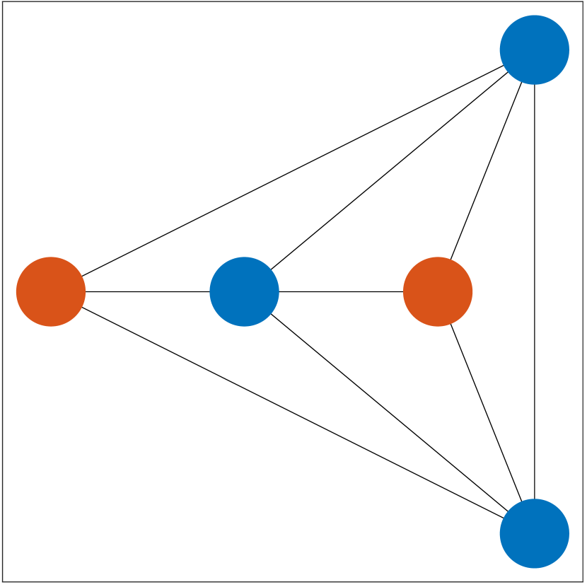
$H_{5,20}$

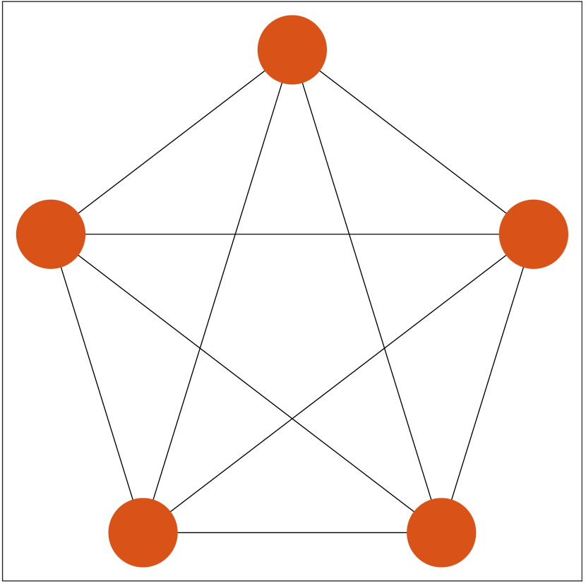
$H_{5,21}$

Figure 5: The penta-node graphlet family $\hat{\mathcal{H}}_{5}$ and family $\mathcal{H}_{5}$. The graphlets $H_{5,p}$, $1\leq p\leq 21$, in $\hat{\mathcal{H}}_{5}$ are mutually non-isomorphic. By the sub-channel decomposition, $\hat{\mathcal{H}}_{5}$ gives rise to 58 orbit-specific graphlets in $\mathcal{H}_{5}$. Orbits are color coded red, blue, green and yellow. For instance, the green orbit of graphlet $H_{5,7,3}$ has two nodes. The graphlets are placed from left to right, top to bottom, by the ordering scheme seira in Section 2.3.

A graph element, a.k.a. graphlet, is a connected template graph with a small number of nodes with or without a designated incidence orbit, see Definitions 2 and 3. All $s$-node graphlets with designated incidence orbits form a natural family ${\cal H}_{s}$, $s\geq 1$. Figure 4 displays the graphlets in the first four families ${\mathcal{H}}_{s}$, $s=1,2,3,4$; Figure 5, the graphlets in family $\mathcal{H}_{5}$. All $s$-node graphlets without orbit partition form the family $\hat{\mathcal{H}}_{s}$, in which all graphlets are mutually non-isomorphic. It is beneficial to utilize smaller graphlets as much as possible for graph encoding. We therefore consider graph encoding with graphlets up to a certain number $t$ of nodes. The length of the frequency-vector code is the sum of the chosen family sizes. For any $s>2$, the size of $\mathcal{H}_{s}$ is $|{\cal H}_{s}|=\sum_{H_{p}\in\hat{\mathcal{H}_{s}}}a_{p}>|\hat{\cal H}_{s}|$, where $a_{p}$ is the number of orbits in pattern template $H_{p}$. Table 1 lists the family sizes up to $8$ nodes. In practice, a small number of graphlet families gives a desirable code length.

Any graphlet collection is a partially ordered set (poset) with the binary relation defined by subgraph inclusion: graphlet $H_{i}$ precedes graphlet $H_{j}$, denoted by $H_{i}\prec H_{j}$, if $H_{i}$ is a proper subgraph of $H_{j}$. The union of the first $t$ families $\mathcal{L}_{t}=\bigcup_{s\leq t}\mathcal{H}_{s}$ is a lattice. Figure 6 shows the Hasse diagram of $\mathcal{L}_{5}$, in which we include the null graph $\emptyset$. The lattice with some of the families removed is a sub-lattice. Alternatively, any family $\mathcal{H}_{s}$, $s\leq t$, together with $\emptyset$, is a sub-lattice. Lattice $\mathcal{L}_{5}$ is a sub-lattice of a larger lattice with more graphlets included. Let $G$ be a source graph. By graph encoding with the graphlets in the first $t$ families, the frequency vector at any vertex $v\in V(G)$ is defined on the lattice $\mathcal{L}_{t}$. The singleton count at any vertex is always $1$, which sums to the total count of nodes in a graph or a subgraph. At each vertex, the lattice $\mathcal{L}_{t}$ with the singleton removed defines the neighborhood architecture. Lattice $\mathcal{L}_{2}$ with the singleton removed is the conventional neighborhood. Extending the degree $d(v)$, the frequency vector at $v$ over $\mathcal{L}_{t}$, $t>2$, quantitatively encodes the multi-order topology structures at the vertex.

We elaborate on a few important details about lattice $\mathcal{L}_{t}$ and its counterpart $\hat{\mathcal{L}}_{t}$. We specify a graphlet $H$ in $\mathcal{L}_{t}$ with an index triplet $(s,p,\sigma)$, $s$ is the number of nodes in $H$, $p$ identifies with a unique topological pattern in $\mathcal{H}_{s}$, and $\sigma$ identifies with a unique orbit of $H$. That is, the graphlet $H_{s,p}$ in $\hat{\mathcal{H}}_{s}$ is expanded, by orbit partition, to the subset $\mathcal{H}_{s,p}=\{H_{s,p,\sigma}\}$ in $\mathcal{H}_{s}$. Figure 7 shows the particular relationship between $\mathcal{H}_{4}$ and $\hat{\mathcal{H}}_{4}$. In $\mathcal{L}_{t}$ or $\hat{\mathcal{L}}_{t}$, the length of the path from any graphlet $H$ to the null element is equal to $m(H)+1$, where $m(H)$ is the number of edges in $H$. The lattice height is $m(K_{t})+1$, where $K_{t}$ is the $t$-node clique. In terms of neighborhood architectures, lattice $\mathcal{L}_{t}$ provides more room for encoding and differentiating orientational information.

Figure 6: The Hasse diagram of lattice $\mathcal{L}_{5}=\{\mathcal{H}_{s},\,1\leq s\leq 5\}$ formed by the subgraph inclusion relationship among graphlets in the first five families. Each node element in the diagram represents a graphlet, except the null graph $\emptyset$ depicted by an un-filled circle to the leftmost. Each edge, directed from left to right, represents the covering relationship. Cliques $K_{s}$, $1\leq s\leq 5$, are depicted with square markers in the central row; non-clique graphlets, with filled circles. The graphlets are color-coded by the families: ${{\cal H}}_{1}$ in cyan, ${{\cal H}}_{2}$ in red, ${{\cal H}}_{3}$ in green, ${{\cal H}}_{4}$ in blue, and ${{\cal H}}_{5}$ in yellow. The number of graphlets in each family is in Table 1. Graphlets with the same path length to the null element are placed in the same vertical layer (at the same location along the horizontal or $x$ axis); they also have the same number of edges. Sub-lattices can be extracted from the lattice, see Figure 7 for two instances. The lattice $\mathcal{L}_{5}$ itself is a sub-lattice of a larger one with more graphlet families included.

We introduce a total ordering scheme, seira, with simple induction rules that are self-contained and extendable. The scheme preserves the inclusion relationship between any two directly comparable graphlets and places a sequential order between any two graphlets non-comparable by inclusion. The ordering between any two graphlets $H_{s,p.\sigma}$ and $H_{s^{\prime},p^{\prime},\sigma^{\prime}}$ is determined by the lexicographic ordering detailed below. [(a)] The integers $s$ and $s^{\prime}$ are naturally ordered.

When $s=s^{\prime}$, we assign a unique integer index to each topologically unique pattern in the same family a unique integer index. That is, $p=p^{\prime}$ if and only if $H_{s,p,\sigma}\cong H_{s,p^{\prime},\sigma^{\prime}}$. We let $p<p^{\prime}$ if $m(H_{s,p,\sigma})<m(H_{s,p^{\prime},\sigma^{\prime}})$, i.e., $H_{s,p,\sigma}$ has a shorter path to the null graph on the Hasse diagram. For example, $K_{1,2}$ is placed ahead of $K_{3}$. In the case of a tie, $m(H_{s,p,\sigma})=m(H_{s,p^{\prime},\sigma^{\prime}})$, we break the tie by the first discrepancy in the frequency sequences (in non-decreasing ordering) drawn from $\{f(H_{k}|H_{s,p,\sigma})\}$ and $\{f(H_{k}|H_{s,p^{\prime},\sigma^{\prime}})\}$, where $H_{k}$ is already placed ahead of $H_{s,p,\sigma}$ and $H_{s,p^{\prime},\sigma^{\prime}}$ by seira itself.

When $(s,p)=(s^{\prime},p^{\prime})$, we assign each orbit a unique integer. That is, $\sigma=\sigma^{\prime}$ if the two graphlets are the one and the same. We let $\sigma<\sigma^{\prime}$ if $f(H_{k}|H_{s,p,\sigma})(v)$ at $v\in\sigma$ is lower than $f(H_{k}|H_{s,p,\sigma^{\prime}})(v^{\prime})$ at $v^{\prime}\in\sigma^{\prime}$ where $H_{k}$ is as described in (b). By the use of frequency codes with precedent graphlets, seira makes quantitative comparisons between two graphlets that are non-comparable by subgraph inclusion. The ordering scheme is used in graphlet placements in Figures 4, 5 and 7 and in matrices composed of graphlet frequencies in Sections 3 and 4. In general, seira can be applied to any collection of graphlets.

2	2	3	1	2	1
1		1		2	4
	1	2	4	6	12
		1		4	12
			1	1	3
				1	6
					1

1				1	1			2	1	3
	1					1			1	1
		1		2	1		2	4	2	6
			1		1	2	2	2	4	6
				1				2		3
					1			2	2	6
						1			2	3
							1	1	1	3
								1		3
									1	3
										1

$\hat{\mathcal{H}}_{4}$

$\mathbf{\hat{U}}_{4}$

${\mathcal{H}}_{4}$

$\mathbf{U}_{4}$

Figure 7: The sub-lattices of $\mathcal{L}_{5}$ for $\hat{\cal H}_{4}$ (left) and ${{\cal H}}_{4}$ (right) and frequency conversion matrices, see ${\cal L}_{5}$ in Figure 6. Matrices $\mathbf{\hat{{U}}}_{4}$ and $\mathbf{{U}}_{4}$, by Definition 4, are shown next to the corresponding sub-lattices. The $p$-th element of the row vector above $\mathbf{\hat{U}}_{4}$ is the size of the $p$-th diagonal block of $\mathbf{U}_{4}$, i.e., the number of orbits in the pattern $H_{4,p}$.

3 Intrinsic connections in frequency vectors

We disclose and describe in this section rich and intrinsically structural connections among the graphlet frequency vectors. These connections are presented coherently and systematically for the first time in simple and rigorous expressions.

3.1 Local transforms on graphlet lattices

Net frequency counting, by Definitions 1, 2 and 3, is subject to the constraint that the subgraphs must be induced. It is shown in a precursor work [14] that with $s$-node graphlet families, $s\leq 4$,

[(i)] counting the gross frequencies of an $s$-node family can be highly flexible, direct and efficient, especially on sparse networks, by utilizing the net or gross frequencies of $s^{\prime}$-node families, $s^{\prime}<s$, and the sparsity structure of a network. The $s$-node frequencies are non-linearly related to the precedent frequencies.

the net frequencies can be obtained with ease and efficiency from gross frequencies within the same family, and vice versa. Specifically, the conversions are by linear transforms.

The two statements extend to any $s$-node graphlet families, $s>2$. They underscore the essential properties common to various formulas in the literature for computing graphlet frequencies. These properties were not declared in previous works elsewhere due in part to the lack of conceptual and computational distinctions between net frequencies and gross frequencies or other possible intermediate frequencies. In the present work, we generalize the finding in (ii) to any graphlet family of $s$-nodes, $s>2$. This finding is important because the linear frequency conversion within any graphlet family leaves the non-linear transforms in graphlet frequencies to that across different families.

In the rest of the section, we focus on intrinsic relations, local to every vertex, in the frequencies w.r.t. graphlets with orbit distinction, i.e., graphlets in families $\mathcal{H}_{s}$, $s\geq 1$. The orbit distinction, however, is not critical; the frequency relations can be translated to the graphlets in $\hat{\mathcal{H}}_{s}$ families by the sub-channel (de)composition property (1). We denote the quantities in $\hat{\mathcal{H}}_{s}$ families with an overhead hat accordingly. Recall from Section 2.3 and Figure 6 the lattices associated with each type of the graphlet families and the relationship between them. The essence in frequency relationships is in the lattice properties.

3.2 Intra-family relations

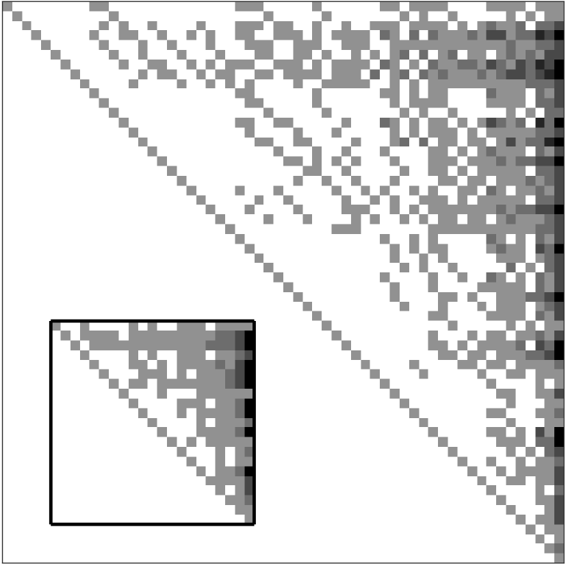
Figure 8: Frequency conversion matrices ${\mathbf{U}}_{5}$ and $\hat{\mathbf{U}}_{5}$ by Definition 4. Elements with larger integers are in darker pixels; with zero values, in white pixels. Both matrices are upper triangular. Matrix $\hat{\mathbf{U}}_{5}$ ($21\times 21$ with $164$ nonzeros) is placed in the lower triangular space of $\mathbf{{U}}_{5}$ ($58\times 58$ with $744$ nonzeros). The inverse of each matrix has the same sparsity pattern, by Theorem 1.

The net frequencies on a source graph $G$ are bounded from above by the corresponding gross frequencies. We prove that with the graphlet encoding system, the net and gross frequency vectors on a source graph w.r.t. to any $s$-node family $\mathcal{H}_{s}$ are related by linear transforms.

Definition 4.

(Intra-family gross-frequency matrices) For any $s>1$, let ${\cal H}_{s}$ be the family of $s$-node graphlets, each with a distinctive incidence orbit. Define matrix $\mathbf{U}_{s}$ by the pairwise gross frequencies among the graphlets in the respective families as follows,

$$\begin{array}[]{l}\mathbf{U}_{s}(i,j)\,\triangleq\,g(H_{i}|H_{j})(v),\quad H_{i},H_{j}\in{\cal H}_{s},\end{array}$$ (2)

where $v$ belongs to the designated orbit of $H_{j}$.

Matrix $\mathbf{U}_{s}$ is intrinsically triangular with unit diagonal values, by the subgraph inclusion in each family and the reflexive property $g(H|H)=1$ with any graphlet $H$; it is therefore unimodular. The matrix is made upper triangular by any ascending (upward) ordering. Its inverse is also upper triangular and unimodular. Matrices $\mathbf{U}_{4}$ and $\hat{\mathbf{U}}_{4}$ are shown in Figure 7. Matrices $\mathbf{U}_{5}$ and $\hat{\mathbf{U}}_{5}$ are depicted as gray images in Figure 8.

Theorem 1.

(Linear conversions of frequency vectors) For $s>1$, let ${\cal H}_{s}$ and $\mathbf{U}_{s}$ be specified as in Definition 4. Then, [(a)] for any source graph $G(V,E)$, at any vertex $v\in V$,

$$\mathbf{U}_{s}\,f({\cal H}_{s}|G)(v)=g({\cal H}_{s}|G)(v);$$ (3)

matrix $\mathbf{U}_{s}\Lambda_{s}$ is involutory, i.e.,

$$\mathbf{U}_{s}^{-1}=\Lambda_{s}\mathbf{U}\Lambda_{s},$$ (4)

where $\Lambda_{s}=\mbox{\rm diag}(\lambda_{i})$ with $\lambda_{i}=(-1)^{m(H_{i})}$, $H_{i}\in\mathcal{H}_{s}$.

By the theorem, net frequencies and gross frequencies w.r.t. the same family $\mathcal{H}_{s}$ are exchangeable via substitution, with any $s\geq 1$. Part (a) of the theorem is straightforward to verify by the definitions of gross and net frequencies. The involutory property of $\mathbf{U}_{s}\Lambda_{s}$ is theoretically interesting in its own right. It is practically useful because the reverse conversions are in the same ready and easy way as the forward conversions in Equation 3.

Proof.

A simple proof of (b) is based on the following fact. Consider $f(H_{i}|G)(v)$, the net frequency at $v$ with respect to template $H_{i}\in{\cal H}_{s}$. We can obtain the net frequency by removing the redundancy from the gross frequency in $g(H_{i}|G)(v)$. For any $H_{j}\succ H_{i}$ covered by $H_{j^{\prime}}$ in the Hasse diagram, the redundancy in $g(H_{i}|G)(v)$ due to $H_{j}$-isomorphic and $H_{j^{\prime}}$-isomorphic subgraphs incident at $v$ is $g(H_{i}|H_{j})g(H_{j}|G)(v)-g(H_{i}|H_{j^{\prime}})g(H_{j^{\prime}}|G)(v)$. By nested removal of the redundancies due to all super-graphs of $H_{i}$, we arrived at,

$$\begin{array}[]{rl}\displaystyle f(H_{i}|G)(v)&=g(H_{i}|G)(v)\displaystyle-\sum_{U(i,j)>0,j\neq i}\lambda_{i}\lambda_{j}\,g(H_{i}|H_{j})\,g(H_{j}|G)(v)\\ &=\lambda_{i}\,U_{s}(i,:)\,\Lambda\,g({\cal H}_{s}|G)(v),\qquad\forall v\in V,\end{array}$$

for any $H_{i}\in{\cal H}_{s}$. ∎

Corollary 2.

Let $\mathbf{U}$ be a matrix in Definition 4. Denote by $\mathbf{U}_{[ij]}$ the sub-matrix obtained from $\mathbf{U}$ with row $i$ and column $j$ removed. Then, $\mathbf{U}_{[ij]}$ is non-singular if and only if $\mathbf{U}(j,i)\neq 0$.

Proof.

By (b) of Theorem 1 and Cramer’s rule, $|\,\mathbf{U}(j,i)\,|=|\,\mathbf{U}^{-1}(j,i)\,|=|\,\det(\mathbf{U}_{[ij]})\,|$. ∎

Proposition 1.

Let $G(V,E)$ be a source graph. For any $s>1$, $H_{j}\in\mathcal{H}_{s}$, at any $v\in V(G)$,

$$f(H_{j}|G)(v)=0\mbox{ \rm if }g(H_{j}|G)(v)<\mathbf{U}_{s}(i,j)\mbox{\rm\ for\ some }H_{i}\in\mathcal{H}_{s},\ H_{i}\prec H_{j}.$$ (5)

The upper bounds in (5) on the precedent gross frequencies are independent of any source graph.

3.3 Inter-family relations

Table 2: Inter-family net-frequency matrix $[\mathbf{W}_{2,4};\mathbf{W}_{3,4}]$, by Definition 6, for filtering by algorithm G-SURF.

	$H_{4,1,1}$	$H_{4,1,2}$	$H_{4,2,1}$	$H_{4,2,2}$	$H_{4,3,1}$	$H_{4,3,2}$	$H_{4,3,3}$	$H_{4,4,1}$	$H_{4,5,1}$	$H_{4,5,2}$	$H_{4,6,1}$
$H_{2,1,1}$	1	3	1	2	1	2	3	2	2	3	3
$H_{3,1,1}$	2	0	1	1	2	1	0	2	2	0	0
$H_{3,1,2}$	0	3	0	1	0	0	2	1	0	1	0
$H_{3,2,1}$	0	0	0	0	0	1	1	0	1	2	3

The relations in frequencies on a source graph across different families are fundamentally non-linear.

Example 1.

For any graph $G(V,E)$, at any $v\in V$,

$$g(H_{4,2,2}|G)(v)\!=g(H_{2,1,1}|G)(v)\,g(H_{3,1,1}|G)(v)-g(H_{3,1,1}|G)(v)-2\,g(H_{3,2,1}|G)(v).$$

We introduce certain useful inference rules by inequalities, regardless how the frequencies with family $\mathcal{H}_{s}$ are computed from the precedent families.

Definition 5.

(Inter-family pairwise-frequency matrices) For $s,s^{\prime}>1$, let ${\cal H}_{s}$ and ${\cal H}_{s^{\prime}}$ be two families of graphlets with distinctive incidence orbits. Define matrix $\mathbf{U}_{s,s^{\prime}}$ and $\mathbf{W}_{s,s^{\prime}}$ by the pairwise gross and net graphlet frequencies, respectively, across the two families,

$$\mathbf{U}_{s,s^{\prime}}(\,i,j\,)\,\triangleq\,g\,(H_{i}|H_{j})(v),\qquad\mathbf{W}_{s,s^{\prime}}(\,i,j\,)\,\triangleq\,f\,(H_{i}|H_{j})(v),\qquad H_{i}\!\in\!\mathcal{H}_{s},\ H_{j}\!\in\!\mathcal{H}_{s^{\prime}},$$ (6)

where $v$ is in the designated orbit of $H_{j}$.

Clearly, when $s^{\prime}=s$, $\mathbf{U}_{s,s^{\prime}}=\mathbf{U_{s}}$ by (2).

Corollary 3.

For $t>1$, let $\widetilde{\mathbf{U}}_{t}\triangleq\big{[}\mathbf{U}_{s,s^{\prime}}\big{]}_{s,s^{\prime}=1}^{t}$ and $\widetilde{\mathbf{W}}_{t}\triangleq\big{[}\mathbf{W}_{s,s^{\prime}}\big{]}_{s,s^{\prime}=1}^{t}$. Then, $\widetilde{\mathbf{U}}_{t}$ and $\widetilde{\mathbf{W}}_{t}$ are block upper triangular and related as follows,

$$\widetilde{\mathbf{W}}_{t}=\mbox{\rm diag}(\mathbf{U}_{1}^{-1},\cdots,\mathbf{U}_{t}^{-1})\,\widetilde{\mathbf{U}}_{t}.$$ (7)

Table 2 shows a submatrix of $\widetilde{\mathbf{W}}_{4}$. Independent of source graphs, matrices $\widetilde{\mathbf{U}}_{t}$ and $\widetilde{\mathbf{W}}_{t}$, for any fixed $t$, can be precomputed once and for all. The relation between them is a direct consequence of Theorem 1.

Proposition 2.

Let $G(V,E)$ be a source graph. For any $s>1$, $H_{j}\in\mathcal{H}_{s}$, at any $v\in V(G)$,

$$f(H_{j}|G)(v)=0\mbox{\rm\ if \ }f(H_{i}|G)(v)<\mathbf{W}_{r,s}(i,j)\mbox{\rm\ for\ some\ }H_{i}\in\mathcal{H}_{r},\ \ r<s.$$ (8)

The upper bounds in (8) on the precedent net frequencies are independent of any source graph.

Remarks. Myriad formulas in the graphlet literature had been used by haphazard selections. We are able to characterize, categorize, relate and interpret them in terms of the relationships among the encoding elements as well as the relationships among graphlet freqencies on any source graph.

4 Algorithm G-SURF

We present a novel algorithm, G-SURF, for systematic and efficient generation of frequency maps on any source graph $G$ with $t$ graphlet families $\mathcal{H}_{s}$, $1<s\!\leq\!t$. We first describe the baseline algorithm. We then elaborate on acceleration methods and show a significant cost reduction in a case study with a real-world network. Additionally, we comment on time and space complexities.

4.1 The baseline algorithm

Algorithm G-SURF takes at input: (i) a source graph $G(V,E)$ with adjacency matrix $A$, and (ii) an integer $t>2$ specifying the graphlet families ${\cal H}_{s}$, $s\leq t$. The algorithm renders at output the net frequency maps $\{f({{\cal H}}_{1:t}|G)(v),v\in V(G)\}$. G-SURF has the following basic steps. Initially, the first net frequency maps are set over $V$,

$$f(K_{1}|G)(V)=1,\quad f(K_{2}|G)(V)=d(V)=A\cdot e.$$

Then, the algorithm iterates sequentially over the graphlet families $\mathcal{H}_{s}$, $s=3,\dots,t$. Step $s$ has two substeps at every vertex $v\in V$:

$$\begin{array}[]{l}\mbox{\tt Compute}\mbox{ gross frequencies}\\ g({\cal H}_{s}|G)(v)=\mbox{\tt upRec}(f({\cal H}_{1:(s-1)}|G)(v),A),\\[6.99997pt] \mbox{\tt Convert}\mbox{ to net frequencies}\\ f({\cal H}_{s}|G)(v)=\mathbf{U}^{-1}_{s}\,g({\cal H}_{s}|G)(v).\end{array}$$

At the first substep, the upward recursion function upRec makes use of the precedent frequencies and adjacency matrix $A$. The upward recursion functions are typically non-linear. There exist various approaches for constructing the recursion function [22, 17, 24, 14], see also Example 1. The construction approaches also vary in how to exploit the structures of $A$, including the sparsity. For the second substep, the transform matrices $\mathbf{U}_{s}$, $s\leq t$, are pre-computed once and for all. At iteration step $s$, the frequency conversion is linear with $n(G)$, the constant prefactor is proportional to $\mbox{nnz}(\mathbf{U}_{s})$. The main cost lies in the upward recursion, which is dominated by the computation of the clique frequencies $g(K_{s}|G)(v)=f(K_{s}|G)(v)$. We introduce next our cost reduction strategies.

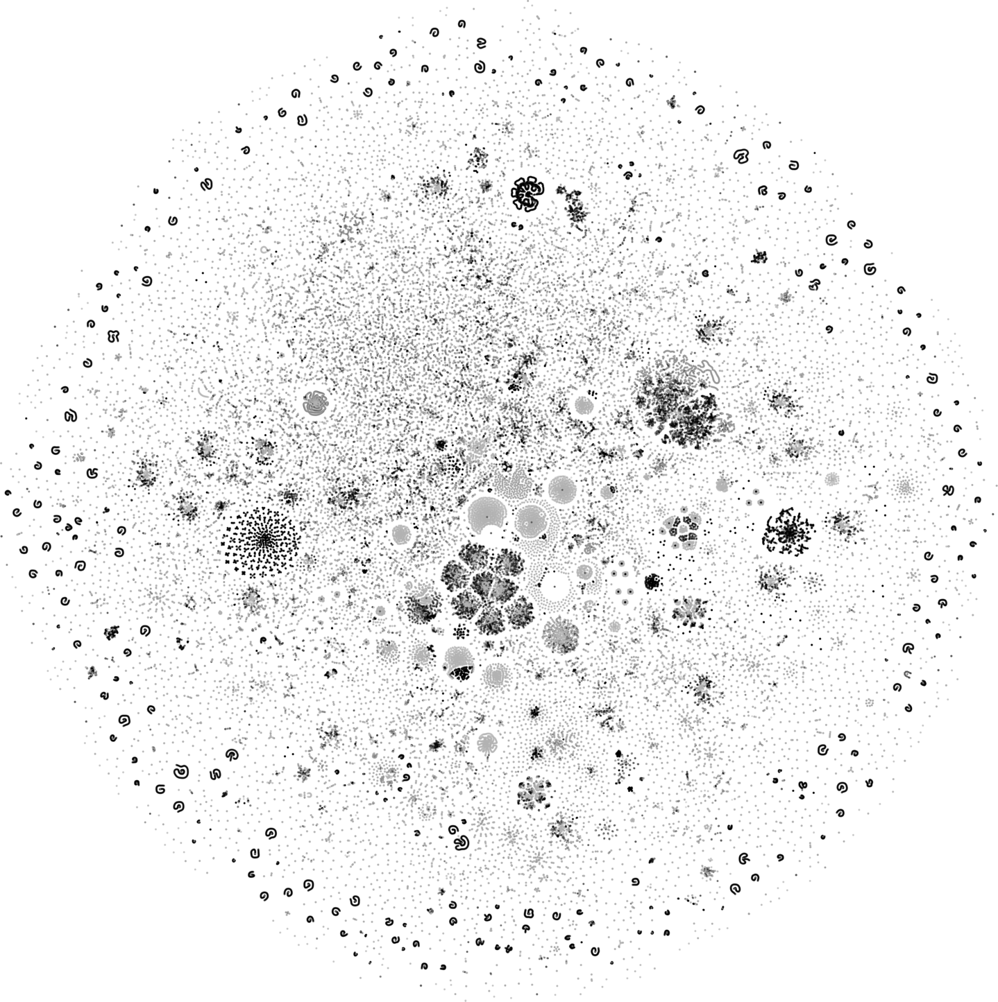
(a)

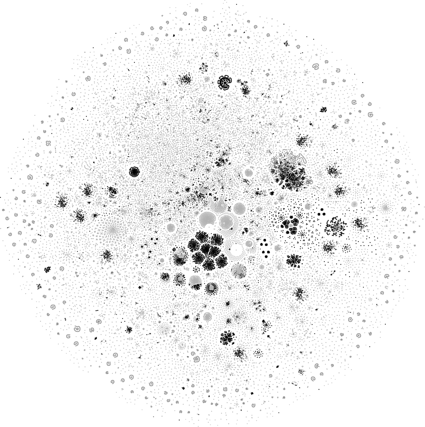
(b)

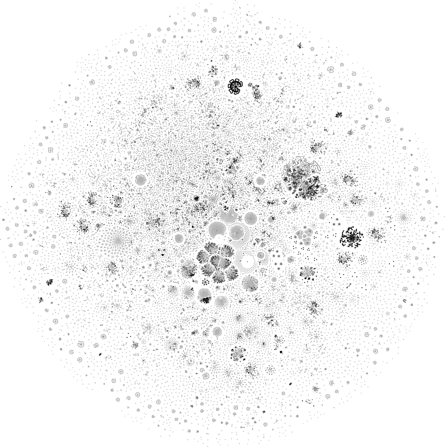
(c)

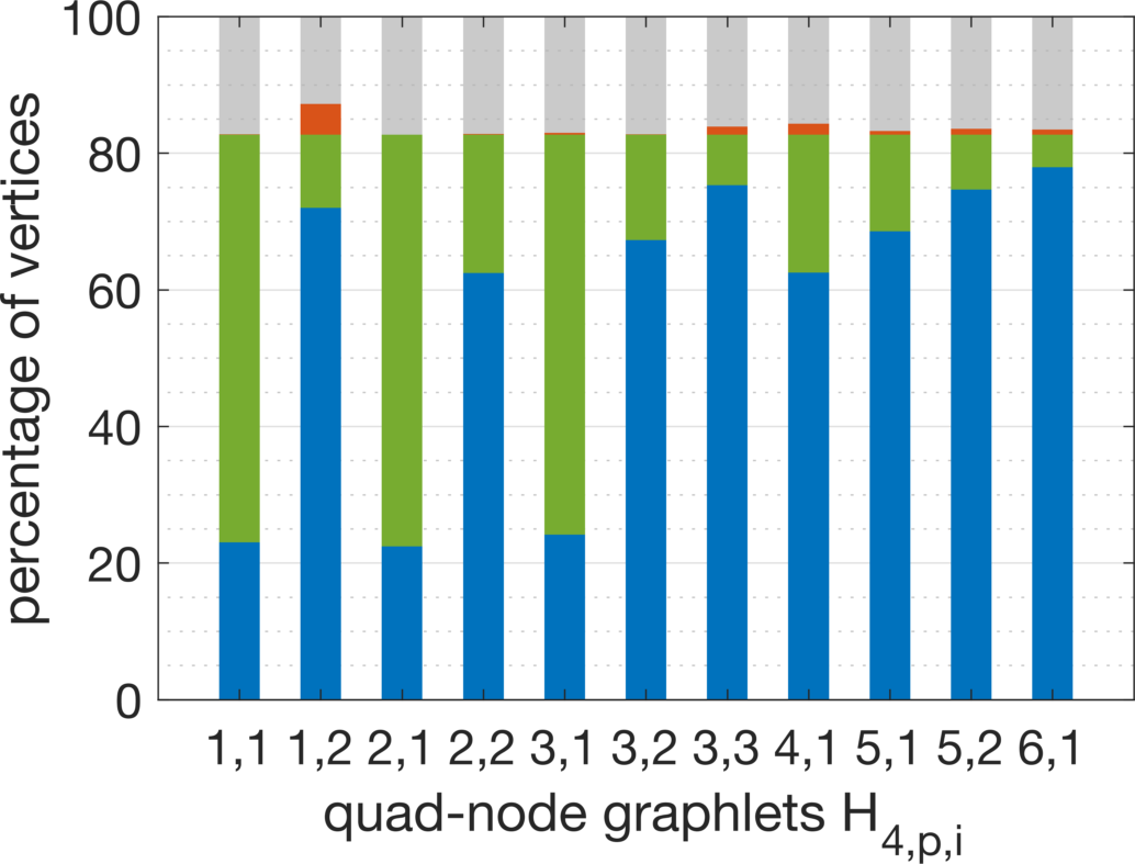
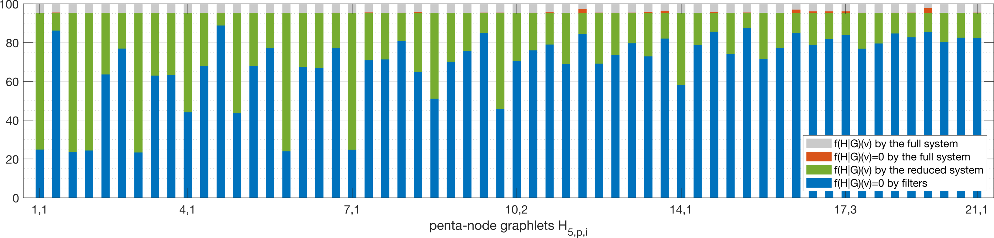
(d)

(e)

Figure 9: Significant reduction in computation cost by algorithm G-SURF on network NotreDame_www. The network, described in Section 4.4, has $325,729$ HTML document nodes and $757,365$ links. (Top): Frequency maps, overlaid on a 2-D spatial embedding of the network [29], with respect to graphlets (a) $H_{4,1,2}$, (b) $H_{4,6,1}$ and (c) $H_{5,4,3}$, respectively. Vertices with zero frequencies are shown in black; non-zeros, in gray. (Bottom): Reduction bar charts with (d) quad-node graphlets and (e) penta-node graphlets. The percentages of vertices (blue) with $f(H|G)(v)=0$ identified by internal filters, (red) with $f(H|G)(v)=0$ identified by full systems, (green) processed by reduced systems, and (gray) processed by full systems. The smaller the grey area is, the more reduction in computation cost. Observation: Reduced systems are used at about $$84$\%$ of the vertices with quad-node graphlets; $$95$\%$, with penta-node graphlets; with larger graphlets, more reduced systems and more cost reduction.

4.2 Reduced systems

At step $s$ we can obtain the clique frequency $f(K_{s}|G)(v)=g(K_{s}|G)(v)$ at vertex $v$ economically if for some $H_{j}\in\mathcal{H}_{s}\!\setminus\!K_{s}$ the frequency $f(H_{j}|G)(v)$ is known prior to the gross-to-net conversion. For instance, if graph $G$ is found path-4 free by a linear-complexity algorithm [9], then $f(H_{4,2}|G)(v)=0$ at all vertices and $f(K_{4}|G)(v)$ can be obtained economically by the following approach. Here, ${\cal H}_{s}\!\setminus\!H$ denotes the set ${\cal H}_{s}$ with $H$ removed. With the additional information of a zero net frequency with $H_{j}$ at $v$, we can reduce the full conversion system (3) at $v$ to the following one by variable substitution, with $H_{j}\neq K_{s}$,

$$\mathbf{U}_{s[sj]}\,f({\cal H}_{s}\!\setminus\!H_{j}|G)(v)=g({\cal H}_{s}\!\setminus\!K_{s}|G)(v).$$ (9)

Here, $\mathbf{U}_{s[ij]}$ is matrix $\mathbf{U}_{s}$ with row $i$ and column $j$ removed, and it is non-singular if $\mathbf{U}_{s}(j,i)\neq 0$, by Corollary 2. In general, under the conditions that $\mathbf{U}_{s}(j,i)\neq 0$ and $i\neq j$, the reduced system with matrix $\mathbf{U}_{s[ij]}$ can be used to infer $f(H_{i}|G)(v)$, with the knowledge of $f(H_{j}|G)(v)$, $H_{i},H_{j}\in\mathcal{H}_{s}$, without calculating the gross frequency $g(H_{i}|G)(v)$.

4.3 Frequency filtering

The system reduction is not limited to external sources of frequency information. The reduced systems are not necessarily uniform across all vertices. We introduce how to infer zero-net frequencies internally for system reduction and make use of precedent frequency information local to each vertex.

At step $s$ of algorithm G-SURF, $M_{s}$ is used as a binary mask over the vertex set $V$. The mask is initially set to zero at all vertices. The algorithm sets $M_{s}(v)=1$ at vertex $v$ when it is recognized that $f(H|G)(v)=0$ for some $H\in\mathcal{H}_{s}$. The system (3) can be reduced at any vertex with $M_{s}(v)=1$. The zero-frequency recognition takes place before and during the computation of the gross frequencies. When the net frequencies with precedent graphlet families, $f({\cal H}_{1:(s-1)}|G)(v)$, become available, matrices $\mathbf{W}_{s^{\prime},s}$, $s^{\prime}<s$, are used to detect zero frequencies, based on Proposition 2. During the computation of gross frequencies, as more information becomes available, the columns of $\mathbf{U}_{s}$ are used to detect zero frequencies from precedent graphlets in the same family, based on Proposition 1. The filtering is self-contained and adaptive to local information.

4.4 Case study & complexities

We present a case study with the real-world network NotreDame_www. The network is the first shown to follow the celebrated Barábasi-Albert model [2]. We treat it as undirected, without self-loops. The resultant network has $325,729$ HTML document nodes and $757,365$ links, with average degree $4.65$. We generate quad-node and penta-node frequency maps using G-SURF. Three of the maps are shown in Figure 9. There is a significant reduction in computation cost. The reduction is measured by the percentage of the reduced systems over the entire vertex set. About $84\%$ of the local systems are reduced for generating the frequency maps with quad-node graphlets; about $95\%$, with the penta-node graphlets. The reduction relies entirely on internal filtering.

We comment on time complexity and space complexity. When the graphlet size is bounded by $t>1$ and when the space complexity is of $O(n^{2})$, G-SURF is of time complexity $O(n^{3})$, under additional assumptions as follows. Matrix multiplications are used in the computation of gross frequencies. Matrix powers $A^{k}$, $1<k\leq t$, may be computed by the square-doubling technique. Asymptotic techniques for matrix multiplications are not used. By this reasoning, the complexity is of the same order as generating the triangle map alone. The hardness level in theoretical worst-case complexity is cubic in time and quadratic in space. In the real world, large networks tend to be sparse. The sparsity shall be exploited to lower both time and space complexities on average over all sparse matrices, which is shown feasible in [14].

5 Discussion

5.1 Relations to previous works

We relate our work to previous works on structures and counts of small subgraphs in a graph or network. To this end, we give a brief overview of the previous works through the lens of our unifying analysis as introduced in the preceding sections. The overview is intended to clarify key distinctions, connections and gaps among the most relevant and notable works, certain lingering faults and limiting factors, and the advance we have made.

Relevant previous works may be categorized first by problem types or objectives and then by solution methodologies. We name below a few problems and describe typical or notable solution methods for each. In a solution method to a particular problem, a connection or translation to another problem may be utilized.

(I) Determine whether or not a graph $G$ is free of certain forbidden connected subgraphs. Such classical graph recognition problems ask whether or not the total count of forbidden subgraphs is zero. Familiar examples include triangle-free, path-free, cycle-free, or diamond-free graphs [12, 19, 9]. A line graph is free of $9$ small subgraph patterns with no more than $6$ nodes each [4, 16]. Specifically, the $9$ patterns are graphlets $H_{4,1}$, $H_{5,17}$, $H_{5,20}$, $H_{6,24}$, $H_{6,58}$, $H_{6,64}$, $H_{6,71}$, $H_{6,91}$ and $H_{6,99}$ by our graph index system. Solution methods for such recognition or detection problems are typically pattern-specific, leveraging the fixed pattern topology and adapting to the local and global connectivity structure in a source graph. Such methods are driven toward optimal time complexity. Remarkably, the algorithm for line-graph recognition and root graph reconstruction by Lehot [21] is of linear complexity with $m(G)$.

(II) Compute the total net counts of small connected subgraphs. Among the notable solution methods are the work by Alon, Yuster and Zwick [3], the work by Kloks, Kratsch and Müller [19] and more recent work by Vassilevska Williams and Williams [35]. These methods are common in their use of fast matrix multiplications for global counting of prescribed small subgraphs. The connections between the template structures are used for the total counts. They are appealing with asymptotically low complexity. However, they remain impractical due to the galactically large prefactor constants.

(III) Find the locations and local counts (i.e., listing) of small cliques in a graph. All nodes in a clique are symmetrical, i.e., any clique has only one orbit. The net count and the gross count of a clique at each vertex are equal. An influential work on clique-listing is by Chiba and Nishizeki [8]. This work also makes a critical link between the subgraph counting complexity and the graph arboricity, the latter is a measure of graph connectivity. Listing cliques up to a fixed size takes polynomial time. The method by Chiba and Nishizeki makes use of sub-clique listings.

(IV) Find the net frequency distributions of graphlets. Graphlets include but are not limited to small cliques. A small graph template with more than one orbits can be split into multiple graphlets. The original concept and use of graphlets are by Pržulj, Corneil and Jurisica [30]. To obtain the graphlet distributions, the graphlet frequency maps are actually obtained first. Unfortunately, the collocation relationships among the frequency maps were discarded in separate extractions for the sequences and distributions, which were examined subsequently for cross-correlations or associations.

Myriad formulas and procedures exist for computing the net frequencies of graphlets [17, 22, 14, 25, 28, 32, 20, 18, 1, 31, 7]. They can be categorized into three types. (1) A type-1 algorithm locates every induced subgraph of a fixed size $t$. The pattern of each induced $t$-node subgraph and its induced subgraphs are then recognized by comparison to the chosen graphlet templates. A type-1 algorithm is expensive, the dominant factor in the algorithm complexity is the number of the induced subgraphs $O(n^{t})$. Common information among overlapping subgraphs is not utilized. (2) A type-2 algorithm starts at every vertex $v$ with the frequency at the smallest graphlets and proceeds by upward recursion to the frequencies with graphlets with one more node. Type-2 algorithms did not have automatically generated equations until a recent work by Melckenbeeck et al. in [25]. The question is left wide open how to choose among various ways to expand by one node the neighborhood of every vertex $v$. (3) A type-3 algorithm leverages neighborhood connections, or walks in network analysis language, by matrix and vector operations [17, 14]. The interpretation of successive matrix-vector products is partially responsible for developing the notion of raw or gross frequencies and for investigating the relationship between gross and net frequencies.

The problem with motif detection and discovery can be described in terms of the above primary problems.

5.2 Potential impacts

The graph encoding system with graphlet frequencies can serve as the ground for a graph calculus. A large problem is presented by small subgraph attributes locally at vertex neighborhoods (differentiation) as well as by their spatial and statistical distributions regionally and globally (integration). A solution to the large graph problem can then be facilitated by a divide and conquer approach. Such ideas and approaches are not new. For example, at the center of the graph matching problem is graph isomorphism. Subgraph analysis is used to facilitate and accelerate graph isomorphism tests [23].

We make another important connection: each of the problems described in Section 5.1 can find its robust, statistical counterparts that are tolerant of errors, noise or perturbation. Such robust property is important to analysis and modeling of real-world networks. A statistical subgraph problem is not necessarily associated with a null model. Applied graph/network problems that can get direct benefits from such graph calculus include community or anomaly detection over a network; graph learning; sampling or pooling on a graph; and graph indexing, search and retrieval which are based on comparison, alignment and matching among networks. The great potential of such graph calculus cannot be underestimated.

References

- [1] Mohammad Al Hasan and Vachik S. Dave “Triangle Counting in Large Networks: A Review” In WIREs Data Mining and Knowledge Discovery 8.2, 2018 DOI: 10.1002/widm.1226
- [2] Réka Albert, Hawoong Jeong and Albert-László Barabási “Diameter of the World-Wide Web” In Nature 401, 1999, pp. 130–131 DOI: 10.1038/43601
- [3] N. Alon, R. Yuster and U. Zwick “Finding and Counting given Length Cycles” In Algorithmica 17, 1997, pp. 209–223 DOI: 10.1007/BF02523189
- [4] Lowell W. Beineke “Characterizations of Derived Graphs” In Journal of Combinatorial Theory 9.2, 1970, pp. 129–135 DOI: 10.1016/S0021-9800(70)80019-9
- [5] Garrett Birkhoff “Lattice Theory”, American Mathematical Society Colloquium Publications 25, 1948
- [6] Garrett Birkhoff “Lattices and Their Applications” In Bulletin of the American Mathematical Society 44, 1938, pp. 793–801 DOI: 10.1090/S0002-9904-1938-06866-8
- [7] Sarra Bouhenni, Saïd Yahiaoui, Nadia Nouali-Taboudjemat and Hamamache Kheddouci “A Survey on Distributed Graph Pattern Matching in Massive Graphs” In ACM Computing Surveys 54.2, 2021, pp. 1–35 DOI: 10.1145/3439724
- [8] Norishige Chiba and Takao Nishizeki “Arboricity and Subgraph Listing Algorithms” In SIAM Journal on Computing 14.1, 1985, pp. 210–223 DOI: 10.1137/0214017
- [9] D.. Corneil, Y. Perl and L.. Stewart “A Linear Recognition Algorithm for Cographs” In SIAM Journal on Computing 14.4, 1985, pp. 926–934 DOI: 10.1137/0214065
- [10] Peter Csermely, Tamás Korcsmáros, Huba J.M. Kiss, Gábor London and Ruth Nussinov “Structure and Dynamics of Molecular Networks: A Novel Paradigm of Drug Discovery” In Pharmacology & Therapeutics 138.3, 2013, pp. 333–408 DOI: 10.1016/j.pharmthera.2013.01.016
- [11] Reinhard Diestel “Graph Theory” 173, Graduate Texts in Mathematics Berlin, Heidelberg: Springer, 2017 DOI: 10.1007/978-3-662-53622-3
- [12] Ralph Faudree, Evelyne Flandrin and Zdeněk Ryjáček “Claw-Free Graphs — A Survey” In Discrete Mathematics 164.1-3, 1997, pp. 87–147 DOI: 10.1016/S0012-365X(96)00045-3
- [13] Dimitris Floros, Tiancheng Liu, Nikos Pitsianis and Xiaobai Sun “Using Graphlet Spectrograms for Temporal Pattern Analysis of Virus-Research Collaboration Networks” In IEEE High Performance Extreme Computing Conference, 2020, pp. 1–7 DOI: 10.1109/HPEC43674.2020.9286161
- [14] Dimitris Floros, Nikos Pitsianis and Xiaobai Sun “Fast Graphlet Transform of Sparse Graphs” In IEEE High Performance Extreme Computing Conference, 2020, pp. 1–8 DOI: 10.1109/HPEC43674.2020.9286205
- [15] Alan George, John R Gilbert and Joseph W. Liu “Graph Theory and Sparse Matrix Computation” New York, NY: Springer, 1993
- [16] Frank Harary and Robert Z. Norman “Some Properties of Line Digraphs” In Rendiconti del Circolo Matematico di Palermo 9, 1960, pp. 161–168 DOI: 10.1007/BF02854581
- [17] Tomaž Hočevar and Janez Demšar “A Combinatorial Approach to Graphlet Counting” In Bioinformatics 30.4, 2014, pp. 559–565 DOI: 10.1093/bioinformatics/btt717
- [18] Chuntao Jiang, Frans Coenen and Michele Zito “A Survey of Frequent Subgraph Mining Algorithms” In The Knowledge Engineering Review 28.1, 2013, pp. 75–105 DOI: 10.1017/S0269888912000331
- [19] Ton Kloks, Dieter Kratsch and Haiko Müller “Finding and Counting Small Induced Subgraphs Efficiently” In Information Processing Letters 74.3-4, 2000, pp. 115–121 DOI: 10.1016/S0020-0190(00)00047-8
- [20] Victor E. Lee, Ning Ruan, Ruoming Jin and Charu Aggarwal “A Survey of Algorithms for Dense Subgraph Discovery” In Managing and Mining Graph Data 40, 2010, pp. 303–336 DOI: 10.1007/978-1-4419-6045-0_10
- [21] Philippe G.. Lehot “An Optimal Algorithm to Detect a Line Graph and Output Its Root Graph” In Journal of the ACM 21.4, 1974, pp. 569–575 DOI: 10.1145/321850.321853
- [22] D. Marcus and Y. Shavitt “RAGE – A Rapid Graphlet Enumerator for Large Networks” In Computer Networks 56.2, 2012, pp. 810–819 DOI: 10.1016/j.comnet.2011.08.019
- [23] Brendan D. McKay and Adolfo Piperno “Practical Graph Isomorphism, II” In Journal of Symbolic Computation 60, 2014, pp. 94–112 DOI: 10.1016/j.jsc.2013.09.003
- [24] Ine Melckenbeeck, Pieter Audenaert, Didier Colle and Mario Pickavet “Efficiently Counting All Orbits of Graphlets of Any Order in a Graph Using Autogenerated Equations” In Bioinformatics 34.8, 2018, pp. 1372–1380 DOI: 10.1093/bioinformatics/btx758
- [25] Ine Melckenbeeck, Pieter Audenaert, Tom Michoel, Didier Colle and Mario Pickavet “An Algorithm to Automatically Generate the Combinatorial Orbit Counting Equations” In PLOS ONE 11.1, 2016, pp. e0147078 DOI: 10.1371/journal.pone.0147078
- [26] R. Milo, Shen-Orr, S., Itzkovitz, S., Kashtan, N., Chklovskii, D. and Alon, U. “Network Motifs: Simple Building Blocks of Complex Networks” In Science 298.5594, 2002, pp. 824–827 DOI: 10.1126/science.298.5594.824
- [27] Stephan Olariu “Paw-Free Graphs” In Information Processing Letters 28.1, 1988, pp. 53–54 DOI: 10.1016/0020-0190(88)90143-3
- [28] Mark Ortmann and Ulrik Brandes “Efficient Orbit-Aware Triad and Quad Census in Directed and Undirected Graphs” In Applied Network Science 2, 2017, pp. 13 DOI: 10.1007/s41109-017-0027-2
- [29] Nikos Pitsianis, Alexandros-Stavros Iliopoulos, Dimitris Floros and Xiaobai Sun “Spaceland Embedding of Sparse Stochastic Graphs” In IEEE High Performance Extreme Computing Conference, 2019 DOI: 10.1109/HPEC.2019.8916505
- [30] N. Pržulj, D.. Corneil and I. Jurisica “Modeling Interactome: Scale-Free or Geometric?” In Bioinformatics 20.18, 2004, pp. 3508–3515 DOI: 10.1093/bioinformatics/bth436
- [31] Pedro Ribeiro, Pedro Paredes, Miguel E.. Silva, David Aparício and Fernando Silva “A Survey on Subgraph Counting: Concepts, Algorithms and Applications to Network Motifs and Graphlets” In ACM Computing Surveys (to appear), 2020
- [32] Takashi Washio and Hiroshi Motoda “State of the Art of Graph-Based Data Mining” In ACM SIGKDD Explorations Newsletter 5.1, 2003, pp. 59–68 DOI: 10.1145/959242.959249
- [33] Duncan J. Watts and Steven H. Strogatz “Collective Dynamics of ‘Small-World’ Networks” In Nature 393, 1998, pp. 440–442 DOI: 10.1038/30918
- [34] Hassler Whitney “Congruent Graphs and the Connectivity of Graphs” In American Journal of Mathematics 54.1, 1932, pp. 150–168 DOI: 10.2307/2371086
- [35] Virginia Vassilevska Williams and R. Williams “Subcubic Equivalences between Path, Matrix, and Triangle Problems” In Journal of the ACM 65.5, 2018, pp. 1–38 DOI: 10.1145/3186893
- [36] Wayne W. Zachary “An Information Flow Model for Conflict and Fission in Small Groups” In Journal of Anthropological Research 33.4, 1977, pp. 452–473 DOI: 10.1086/jar.33.4.3629752