Enhancing Robustness of On-line Learning Models on Highly Noisy Data

Abstract

Classification algorithms have been widely adopted to detect anomalies for various systems, e.g., IoT, cloud and face recognition, under the common assumption that the data source is clean, i.e., features and labels are correctly set. However, data collected from the wild can be unreliable due to careless annotations or malicious data transformation for incorrect anomaly detection. In this paper, we extend a two-layer on-line data selection framework: Robust Anomaly Detector (RAD) with a newly designed ensemble prediction where both layers contribute to the final anomaly detection decision. To adapt to the on-line nature of anomaly detection, we consider additional features of conflicting opinions of classifiers, repetitive cleaning, and oracle knowledge. We on-line learn from incoming data streams and continuously cleanse the data, so as to adapt to the increasing learning capacity from the larger accumulated data set. Moreover, we explore the concept of oracle learning that provides additional information of true labels for difficult data points. We specifically focus on three use cases, (i) detecting 10 classes of IoT attacks, (ii) predicting 4 classes of task failures of big data jobs, and (iii) recognising 100 celebrities faces. Our evaluation results show that RAD can robustly improve the accuracy of anomaly detection, to reach up to 98.95% for IoT device attacks (i.e., +7%), up to 85.03% for cloud task failures (i.e., +14%) under 40% label noise, and for its extension, it can reach up to 77.51% for face recognition (i.e., +39%) under 30% label noise. The proposed RAD and its extensions are general and can be applied to different anomaly detection algorithms.

I Introduction

Anomaly detection is one of the core operations for enforcing dependability and performance in modern distributed systems [Xue:TNSM18:Ticket, DBLP:journals/tpds/PhamWTBTKI17]. Anomalies can take various forms including erroneous data produced by a corrupted IoT device or the failure of a job executed in a datacenter [Birke:TNSM16:Cloud, BirkeDSN2014, Zhao:DSN19].

Dealing with this issue has often been done in recent art by relying on machine learning-based classification algorithms over system logs [Fang:2010, Giantamidis:2016] or backend collected data [DBLP:conf/ijcai/ZhangLSLH19, Huang:2017]. These systems often rely on the assumption of clean datasets from which the classifier learns to distinguish between data corresponding to a correct execution of the system from data corresponding to an abnormal execution of the latter (i.e., anomaly detection). As workloads at real systems are highly dynamic over time, it is even more challenging to predict anomalies that can not be easily distinguished from the system dynamics, compared to the systems with static workloads.

In this context, a rising concern when applying classification algorithms is the accessibility to a reliable ground truth for anomalies [Cerf:NIPsWS18:Duao]. Typically, anomaly data is manually annotated by human experts and hence the generation of anomaly labels is subject to quality variation, so-called noisy labels. For instance, annotating service failure types for data centers is done by operators of varying expertise.

However, standard machine learning algorithms typically assume clean labels and overlook the risk of noisy labels. Moreover, recent studies point out the increase in dirty data attacks that can maliciously alter the anomaly labels to mislead the machine learning models [Kang:2018, Fan:2018, He:2017, tps2019]. As a result, anomaly detection algorithms need to capture not only anomalies that are entangled with system dynamics but also the unreliable nature of anomaly labels.

Indeed, a strong anomaly classification model can be learned by incorporating a larger amount of data. However, learning from data with noisy labels can significantly degrade the classification accuracy, even for deep neural networks [Vagin:2011, DBLP:conf/iclr/ZhangBHRV17, tps2019]. Such concerns lead us to ask the following question: how to build an anomaly detection framework that can robustly differentiate between true and noisy anomalies and efficiently learn anomaly classification models from a succinct amount of clean data. The immediate challenge of capturing the data quality lies at the fact that label qualities are not directly observable but only via anomaly classification outcomes that in turn are coupled with the noise level in data labels.

We extend Robust Anomaly Detector (RAD) [Zhao:DSN19], a generic framework that continuously learns an anomaly classification model from streams of event logs or images that are subject to label noise. The original design of RAD is composed of two layers of learning models, i.e., a data label model and an anomaly classifier. The label model aims at differentiating the label quality, i.e., noisy v.s. true labels, for each batch of new data and only “clean” data points are fed in the anomaly classifier. The anomaly classifier predicts the event outcome that can be divided in multiple classes of (non)anomalies, depending on the specific use case. In this extension, we derive three alternatives of RAD, namely, voting, active learning and slim. These use additional information, e.g., opinions of conflicting classifiers and queries of oracles. We iteratively update the prediction of historical windows such that weak predictions can be continuously improved by the latest model. Moreover, we propose an ensemble prediction strategy to reconcile the prediction outcomes of the two models, namely label model and anomaly classification model, instead of only relying on classification model as [Zhao:DSN19]

To demonstrate the effectiveness of RAD, we consider three use cases using open datasets: detecting 10 classes of attacks on IoT devices [meidan2018n], predicting 4 types of task failures for big data processing cluster [reiss2011google, Rosa-DSN15], and recognising 100 most abundant celebrity faces [facescrub:2014]. Our results show that RAD can effectively cleanse the data, i.e., selecting data with clean labels, and result in better anomaly detection accuracy per additional included streamed data, compared to classifiers without continuous data cleansing. Specifically, under 40% noise, RAD achieves up to 98.95%, 85.03% (comparing to 92.27% and 71.02% by anomaly classification model of no selection on dataset) for detecting IoT device attacks and predicting cluster task failures, respectively. If we implement RAD Active Learning on cluster dataset with the same noise level, the final accuracy could improve from 85.03% to 90.77%. For face image dataset, final accuracy of RAD Slim under 30% noise achieves to 77.51% (comparing to 38.89% of no selection on dataset). Furthermore, our study shows that RAD is stable even when the noise is very strong. And if we do not have many clean data at beginning to pre-train the model, RAD Active Learning and RAD Active Learning Limited can still perform very well from a very bad starting model.

The main contributions of this study can be summarized as follows:

• We design an effective on-line anomaly detection framework, RAD, consisting of a data selection and prediction module that cater to a wide range of implementation choices from regular machine learning models to deep neural networks.

• We explore three novel data selection schemes: namely voting, active learning, and active learning limit. These can filter out the suspicious data and call upon experts to cleanse the data based on the predicted uncertainty from the quality model and classification model. We combine the novel ideas of model disagreement and active learning.

• We leverage the power of ensemble model prediction to enhance the robustness of trained anomaly classifier by incorporating the predictions of the label model used in the data selection.

• RAD can be applied on multiple types of anomaly inputs, i.e., server failure, IoT devices, and images. Specially, RAD Active Learning can achieve remarkable accuracy similar to the performance under no label noise.

The remainder of the paper is organized as follows. Section III describes the motivating case studies. Sections IV and LABEL:sec:Evaluation present the proposed RAD framework and the results of its experimental evaluation, respectively. Section II describes the related work. Finally, Section LABEL:sec:Conclusion draws our conclusions.

II Related Work

Machine learning has been extensively used for failure detection [Pitakrat:2013, Pellegrini:2015, Reuter:2018, Campos:2018], attack prediction [Agarwal:2016, Banescu:2017, Anbar:2018, Kozik:2018, Karagiannis:2018, Zhou:2018], and face recognition [DBLP:conf/cvpr/TaigmanYRW14, DBLP:conf/cvpr/SchroffKP15, DBLP:conf/cvpr/WangWZJGZL018]. Considering noisy labels in classification algorithms is also a problem that has been explored in the machine learning community as discussed in [Frenay:TNNLS14:survey, biggio2011support, natarajan2013learning].

The problem of classification in presence of noisy labels can be organized into various categories according to, on the one hand, the type of classification algorithm subject to noise, and on the other hand, the techniques used to remove the noise.

Noisy labels have been studied for binary classification where noisy labels are considered as symmetric (e.g., [larsen1998design]) and for classification with multiple classes where noisy labels are considered as asymmetric, e.g., [patrini2017making, sukhbaatar2014training]. For this paper, we consider the problem of classification with multiple classes. Furthermore, noisy labels have been considered in various types of classifiers KNN [Wilson:ML2000:MLselection], SVM [An:Neurocomput.13:SVM], and deep neural networks [Vahdat:NIPS17:NoisyLabelDNN]. In the context of this paper, our proposed approach is agnostic to the underlying classifier type as noise removal is performed ahead of the classification.

Various techniques explore countering label noise following two main strategies. The first strategy trains a single model as filter for noisy label data. [Agarwal:2016, veit2017learning, li2017learning, Dan:nips2018:Using] train a separate filter from clean data for distinguishing noisy labels. Instead [DBLP:conf/apweb/ThongkamXZH08] trains on the original data (with noise). Training the filter with clean data is better, but the assumption of large quantity of clean data does not always hold, especially in our on-line learning scenario. Using noisy data to train a filter raises a chicken-and-egg dilemma [Frenay:TNNLS14:survey], since: 1) good classifiers are necessary for filtering but 2) learning from noisy label data may precisely produce poor classifiers.

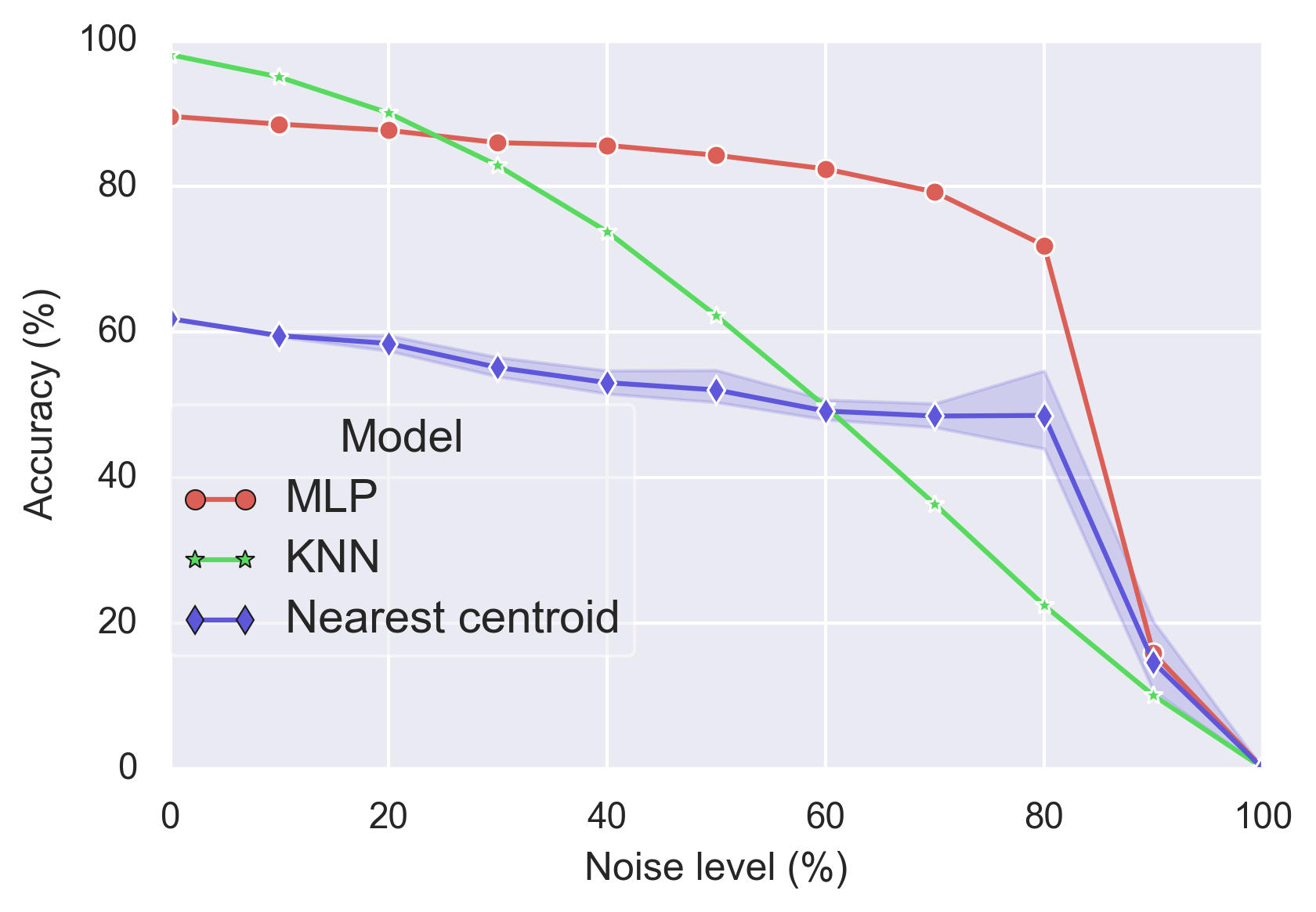
(a) Use case of IoT thermostat device attacks

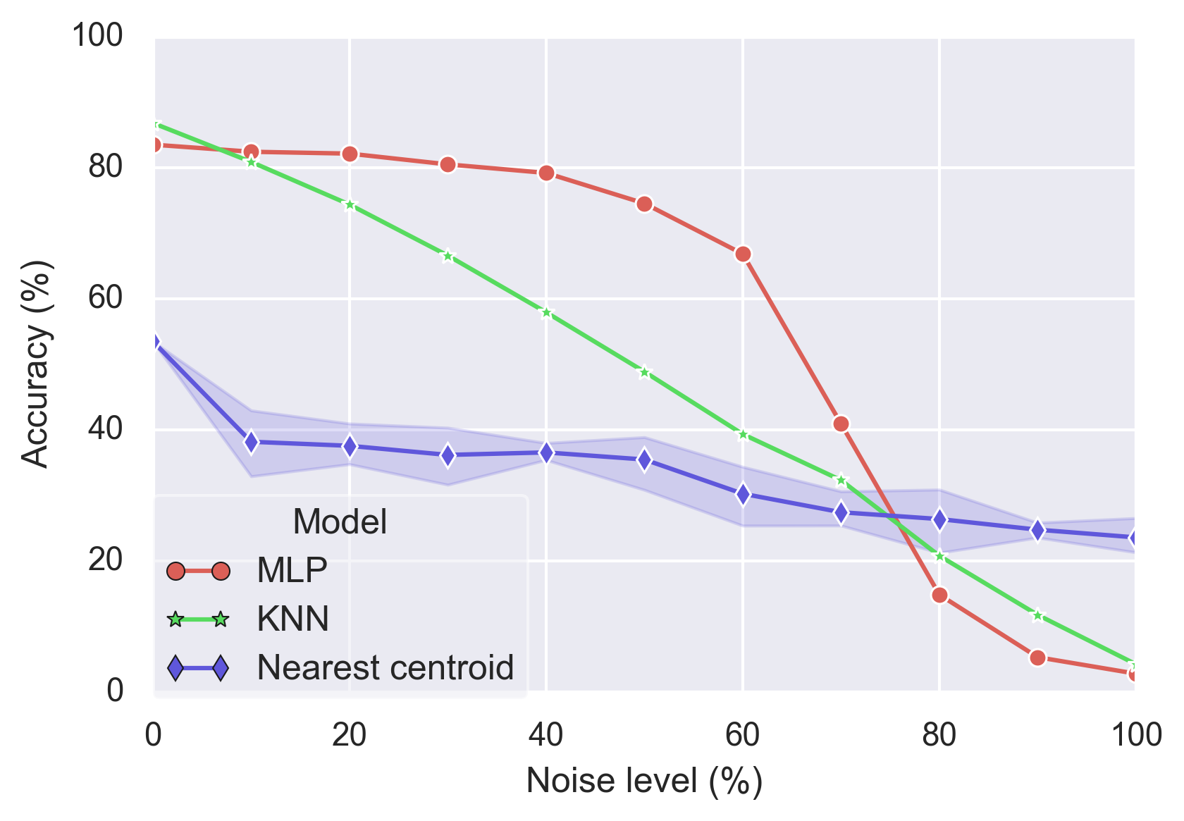
(b) Use case of Cluster task failures

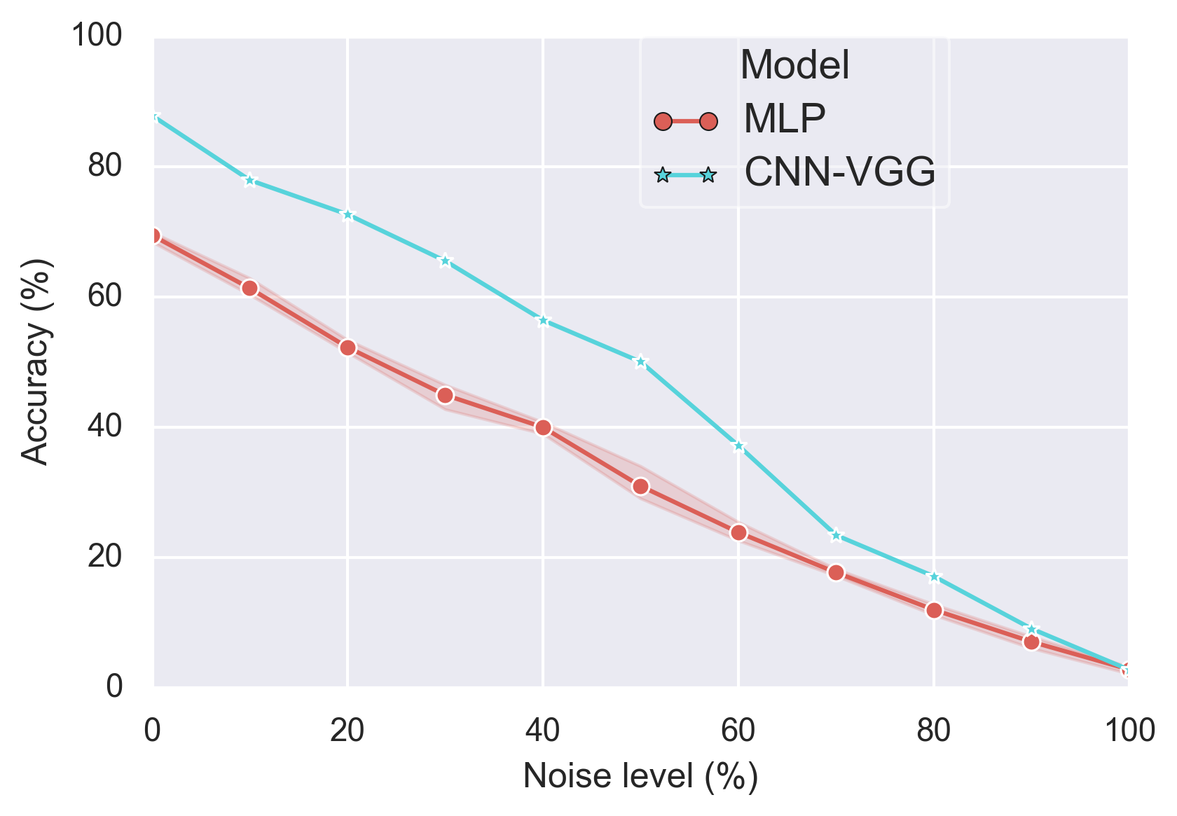
(c) Use case of Face Recognition

Figure 1: Impact of noisy data on anomaly classification

The second strategy relies on voting based algorithms to mitigate possible biases stemming from a chosen single filter. [brodley1996, DBLP:conf/hais/MirandaGCL09, piyasak2010] simultaneously train several classifiers directly on the original data. Afterwards, they use either majority vote (i.e. classify a sample as mislabeled if a majority of classifiers misclassified it) or consensus vote (i.e. classify a sample as mislabeled if all classifiers misclassified the sample) to filter noisy data. There are similarities between these algorithms and our RAD Voting and RAD Active Learning. However, these solutions focus on static datasets and the off-line setting. They do not consider the learning efficiency and training limitation for on-line scenarios. Since the interval between data batches can be short, we need to ensure the training and inference times per batch are as short as possible. The two models in our RAD are connected in cascade. Only data instances deemed uncertain by the first model get to be predicted twice. Off-line voting methods instead need to process each data record multiple times, once for each classifier trained by the algorithm. [piyasak2010] trains two neural networks on top of the classification model. In image classification, training three big CNNs can be hardware-impossible on many devices or very slow and not suitable for on-line learning.

Using active learning in data cleaning has been explored in pattern recognition research. [guyon1994] proposes to define an information criteria function for patterns (data instances). If the information value is below a given threshold, the pattern can be used by the learning algorithm. Otherwise, the pattern is sent to a human expert for checking. The idea is similar to our active learning method, but we go one step beyond by limiting the number of expert queries and proposing an uncertainty-based ranking in RAD Active Learning Limited and RAD Slim Limited. Only the most valuable instances are thus selected to expert cleansing.

III Motivating case studies

To qualitatively demonstrate the impact of noisy data on anomaly detection, we use three case studies.

• Detecting IoT device attacks from inspecting network traffic data collected from commercial IoT devices [meidan2018n]. This dataset contains nine types of IoT devices which are subject to 10 types of attacks. Specifically, we focus on the Ecobee thermostat device that may be infected by Mirai malware and BASHLITE malware. Here we focus on the scenario of detecting and differentiating between 10 attacks. It is important to detect those attacks with high accuracy against all load conditions and data qualities.

• Predicting task execution failures for big data jobs running at a Google cluster [reiss2011google, Rosa:TSC17:failurePrediction]. This trace contains a month-long job execution records from Google clusters. Each job contains multiple tasks, which can be terminated into four different states: finish, fail, evict, or kill. The last three states are considered as anomalous states. To minimise the computational resource waste due to anomalous states, it is imperative to predict the final execution state of task upon their arrivals.

• Recognizing celebrity faces from photos of the FaceScrub dataset [facescrub:2014]. The set is a collection of photos of celebrities roughly half female and half male. The task is to recognize faces by matching each photo to the identity of the celebrity shown on it. Here we focus on the face recognition of the 100 celebrities with the highest number of photos in the dataset totalling to 12K images. Faces are widely used in biometric identification systems in many security applications, e.g., access control. This makes the robustness of such systems critical. Furthermore, this image dataset is studied because we want to show the broad applicability of our proposed framework.

The details about data definition, and statistics, e.g., number of feature and number of data points, can be found in Section LABEL:ssec:Datasets. To recognize anomalies/faces in each use case, related studies have applied different machine learning classification algorithms, from simple ones, e.g., k-nearest neighbour (KNN), to complex ones, e.g., deep neural networks (DNN), under scenarios with different levels of symmetric label noise. Noisy labels are corrupted with equal probability to all classes except the true one. Here, we evaluate how the detection accuracy changes relative to different levels of noises. We focus on off-line scenarios where we split the data in a training set affected by label noise and a clean evaluation set. Due to our focus on resistance to noisy labels, we repeat experiments by regenerating the noise while keeping the model initialisation constant.

III-A Anomaly Detection

Classification models are learned from 14,000 training records and evaluated on a clean testing set of 6,000 records. We specifically apply KNN, nearest centroid and multilayer perceptron (MLP) (a.k.a feed-forward deep neural networks) on both the IoT device attacks and the cluster task failures. We repeat all experiments 10 times. Fig. 1a and Fig. 1b summarize the accuracy results.

One can see that noisy labels clearly deteriorate the detection results for both IoT attacks and task failures, across all three classification algorithms. For standard classifiers, like KNN and nearest centroid, the detection accuracy decays faster than MLP which is more robust to noisy labels. Such an observation holds for both use cases. For IoT attacks, MLP can even achieve a similar accuracy as the no label noise case, when 40% of label classes are altered. Moreover, the impact of noise depends also heavily on the specific sequence of label noise. Corrupting the labels of some samples has a higher impact than corrupting others. As a consequence the curve is highly unstable with large variances and leads sometimes to counter intuitive results of non monotonic impact of noise level on accuracy. An example is given by the nearest centroid results on the cluster task dataset. Even across 100 runs the mean accuracy at 30% noise is slightly lower than the mean accuracy at 40% noise.

III-B Face Recognition

For face recognition we use a subset of our complete dataset (which contains 100 celebrities). The subset contains 2,639 images from 20 celebrities with varying degrees of label noise as training set and 665 clean images as testing set. Due to the complex features of image data, we use a MLP and convolutional neural networks (CNN). Specifically we use a small VGG [Simonyan15] with 6 convolutional layers. We repeat MLP experiments 10 times, and VGG experiments 3 times due to the higher training complexity. Fig. 1c shows the accuracy results under different label noise levels. Similar to previous use cases, one can observe that label noise strongly affects the performance of both classifiers. The accuracy degradation is approximately linear with the noise level. VGG outperforms MLP in this dataset under all noise levels except 100% corrupted labels.

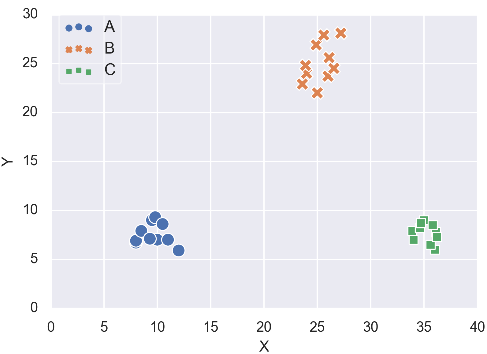
(a) Original data

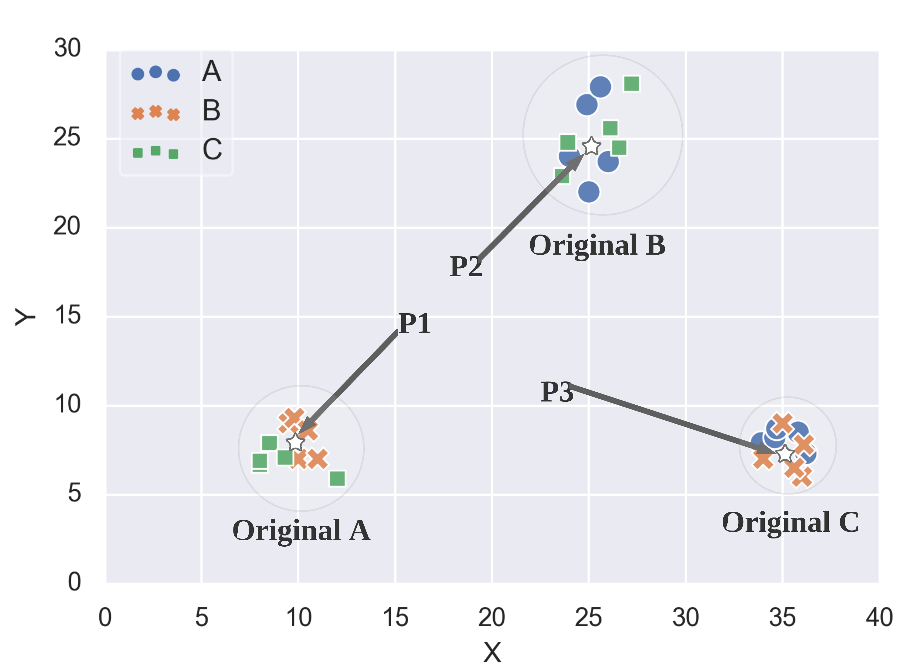
(b) 100% noisy label data

Figure 2: Example of training under 100% label noise.

Although it is rare to encounter a dataset with 100% noisy labels, it is still an interesting scenario to study. Almost all accuracy curves in Fig. 1 reach near 0% under 100% noise. This can be counter intuitive as illustrated by the following example. If the dataset contains $K$ balanced classes, one might think that it should be possible to obtain an accuracy of $\frac{1}{K}$ just by guessing. However training on 100% noisy label data is worse than random guessing. We illustrate this via a simple example with three classes, A, B and C, and 10 samples per class. Fig. 2a shows the original sample distribution. Fig. 2b shows the sample distribution with 100% label noise. Since all labels are corrupted, each original cluster only contains labels of wrong classes. If we train a machine learning model (e.g., KNN with $k=5$) on this noisy label data, we learn a wrong model which can misclassify any data point. See the highlighted points P1, P2 and P3 in Fig. 2b as examples. Training on 100% noisy label data is hence worse than zero-knowledge guessing because fully corrupted data can mislead the learning process.

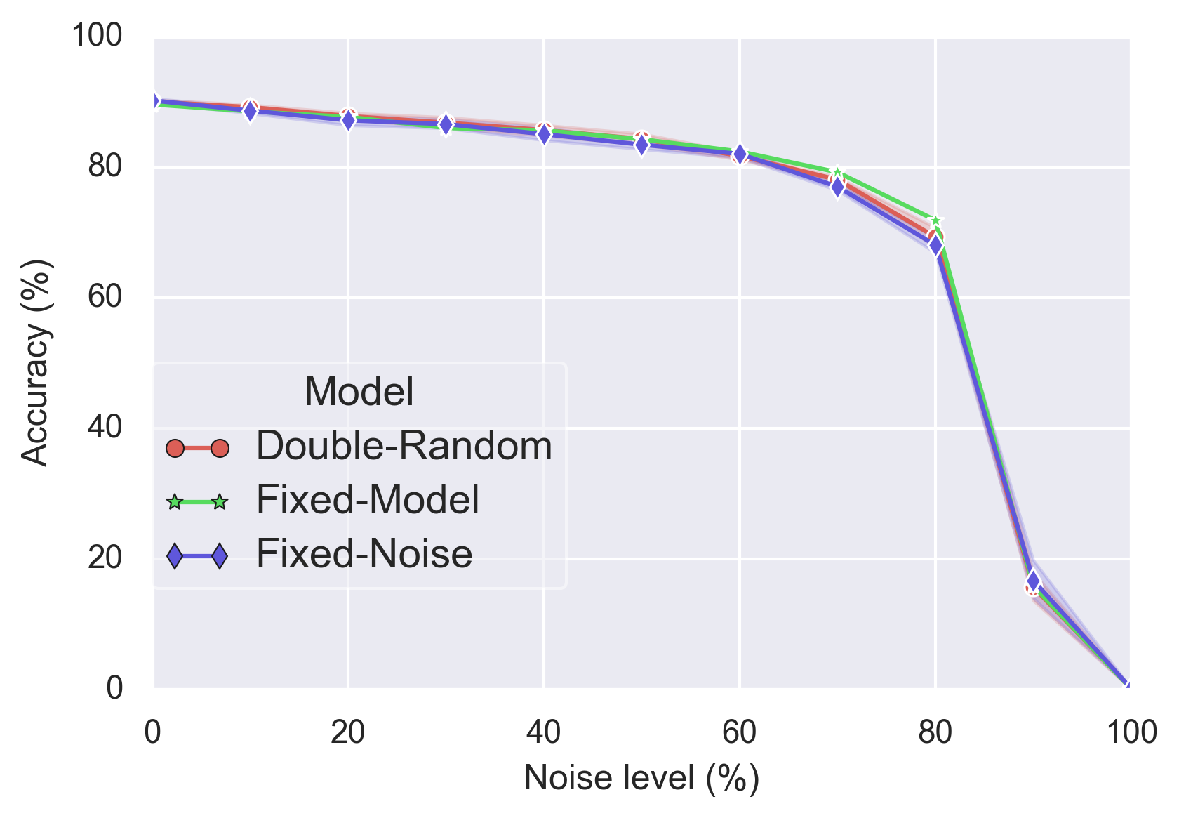
(a) IoT attack

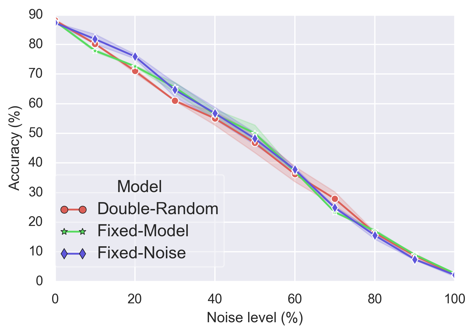
(b) Face recognition

Figure 3: Impact of model vs. noise randomness across runs.

We fix the model initialization and regenerate the noisy data across experiment runs. The randomness of the results only stems from the noise injected into the data labels used for training. Before choosing this setting, we run preliminary experiments with different types of randomness. Fig.3 shows the results on the IoT attack and Face recognition datasets using MLP and VGG, respectively. It compares: Fixed-Model initialization with regenerated noise – our setting throughout the paper; Fixed-Noise with random model initialization; and Double-Random with regenerated noise and random model initialization. Both cases show significant overlaps between the three types of randomness, especially for MLP. Due to the lower number of runs (3 against 10) and higher model complexity, the VGG results are slightly more dispersed. Neither case shows significant impact of the randomness type on the results. As our study focuses on the influence of noisy label data, we choose Fixed-Model for the remainder of the paper.

The above three experiments clearly show that under the presence of noisy label data, all models are progressively degraded. These cases motivate us to design the RAD framework and its extension to counter the influence of noisy label data on the learning process.

IV Design Principles of RAD Framework

In this section, we introduce the system model followed by the general structure of RAD and its extended features with respect to data selection and model prediction – ensemble prediction. All used symbols are summarized in Table I.

IV-A System Model

We consider a dataset that consists of several data instances. Each data instance has $f$ features. Each data instance belongs to a class $k$, where $k\in\mathcal{K}=\{1,\dots,\textit{K}\}$. Data instances are part of a pre-labeled dataset $\mathcal{D}$ with labels $Y$ used for training. Furthermore, a labeled data instance is either correctly labeled (i.e., clean data instance), or incorrectly labeled (i.e., noisy data instance). We use the indicator variable $\hat{q}$ to indicate clean $\hat{q}=1$ and dirty $\hat{q}=0$ labels. Wrong labels can stem from several reasons ranging from subjectivity and data-entry errors, to malicious error injection. The quality of a dataset $\mathcal{D}$ is measured as the percent of clean labeled data instances, denoted here as $\tilde{Q}$.

TABLE I: Symbol description

Symbol	Description
$\mathfrak{L}$	label quality predictor
$\mathfrak{C}$	anomaly detection classifier
$\mathcal{D}_{i}$	$i^{th}$ training data batch
$\mathcal{D}_{i}^{*}$	$i^{th}$ cleansed data batch from $\mathfrak{L}$
$\mathcal{P}_{i}$	$i^{th}$ test data batch
$\hat{Y}_{i}$	prediction of $i^{th}$ test data batch from $\mathfrak{C}$
$\tilde{Q}_{i}$	percent of clean labeled data of $i^{th}$ batch
$\mathcal{U}_{i}$	“unclean” data of $i^{th}$ batch determined by $\mathfrak{L}$
$\mathcal{U}_{i}^{*}$	$i^{th}$ cleansed data batch from $\mathfrak{C}$
$\mathcal{S}_{i}$	“unclean” data of $i^{th}$ batch determined by $\mathfrak{C}$
$\mathcal{S}_{i}^{*}$	data with true label from Expert of $i^{th}$ batch
$\hat{p}$	indicator of prediction, 1 for clean, 0 for dirty
$\hat{q}$	indicator of prediction, 1 for clean, 0 for dirty
$\alpha$	accuracy on testing set

Data instances arrive at the learning system continuously over time in batches. $\mathcal{D}_{i}$ denotes the batch of labeled data arriving at time $t_{i}$ and having labels $Y_{i}$. In general we denote the time window with the subscript $i$. We assume that a small initial batch of data instances $\mathcal{D}_{0}$ has only clean labels, that is $\tilde{Q}_{0}=100\%$. Subsequent batches, include varying proportions of noisy labels, i.e $0<\tilde{Q}_{i}<100\%,i>0$. For simplicity we consider arriving batches of equal size, $\forall\mathcal{D}_{i},|\mathcal{D}_{i}|=N$, but not necessarily at regular times.

A classification request consists of a batch of non-labeled data instances $\mathcal{P}_{i}$ for which the classifier predicts the class $k$ of each data instance. At each batch arrival, the classification output $\hat{Y}_{i}$ is thus an array of the predicted classes for each non-labeled data instance.

IV-B Design Overview of RAD

We propose the RAD learning framework. Its objective is threefold:

1. Learn accurate models from noisy data.

2. Continuously update the learned models based on new incoming data.

3. Propose a general approach that fits to different machine learning algorithms and different application use cases.

RAD is composed of two key steps: training data selection and class prediction, as shown in Fig. 4. Training data selection focuses on how to filter out suspicious noisy data instances and solicit clean data to subsequently train the classification model. It has four options: basic, voting, active and slim. The class prediction uses different prediction techniques. Available options are ensemble, which combines the prediction outcomes of quality and classification models; and slim, which has only one model to filter and classify anomalous images. We consider the following specific combinations: (i) basic, voting, and active are followed by the ensemble prediction; (ii) slim is followed by the slim prediction, which only uses one model to save computation resources.

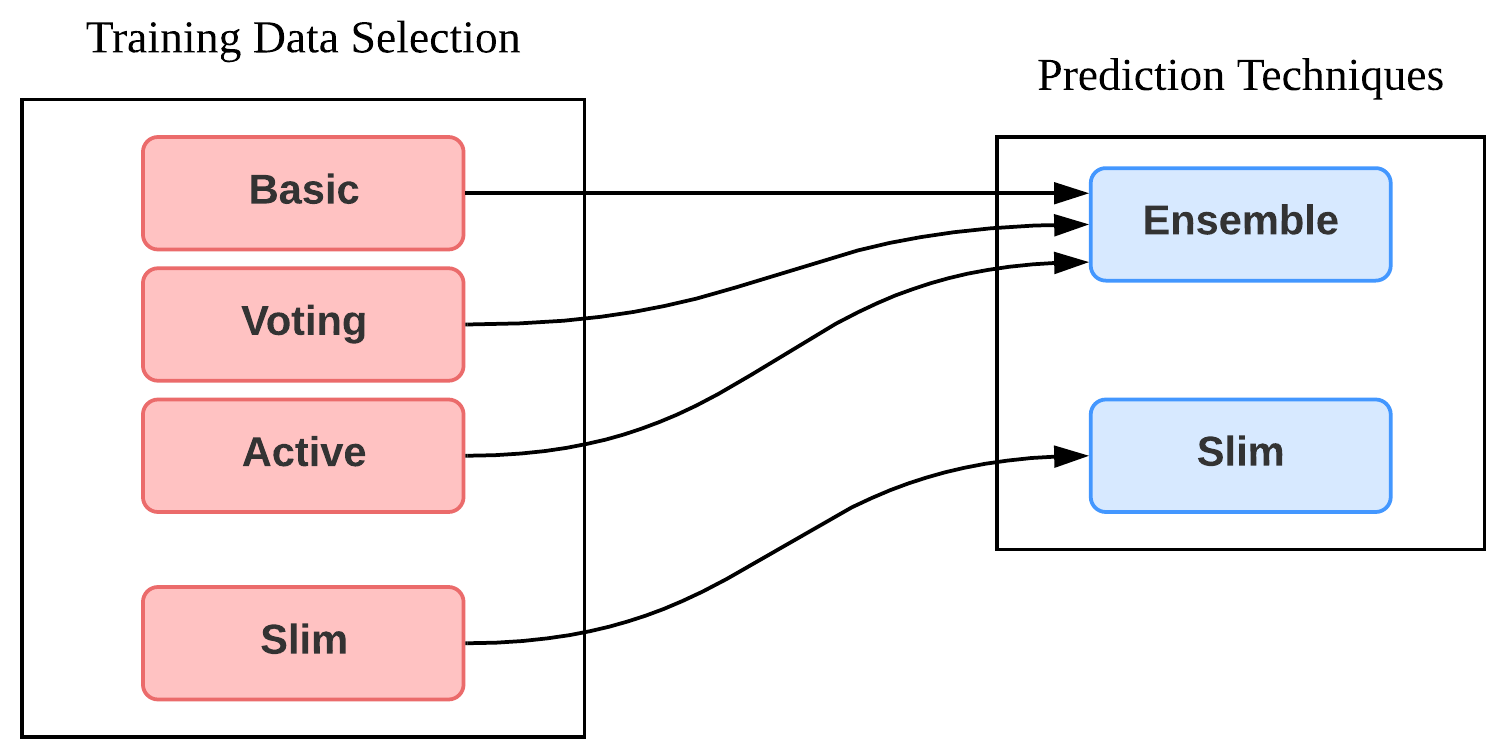
Figure 4: Structures of RAD and its extensions: four choices of data selection and two choices of class prediction.

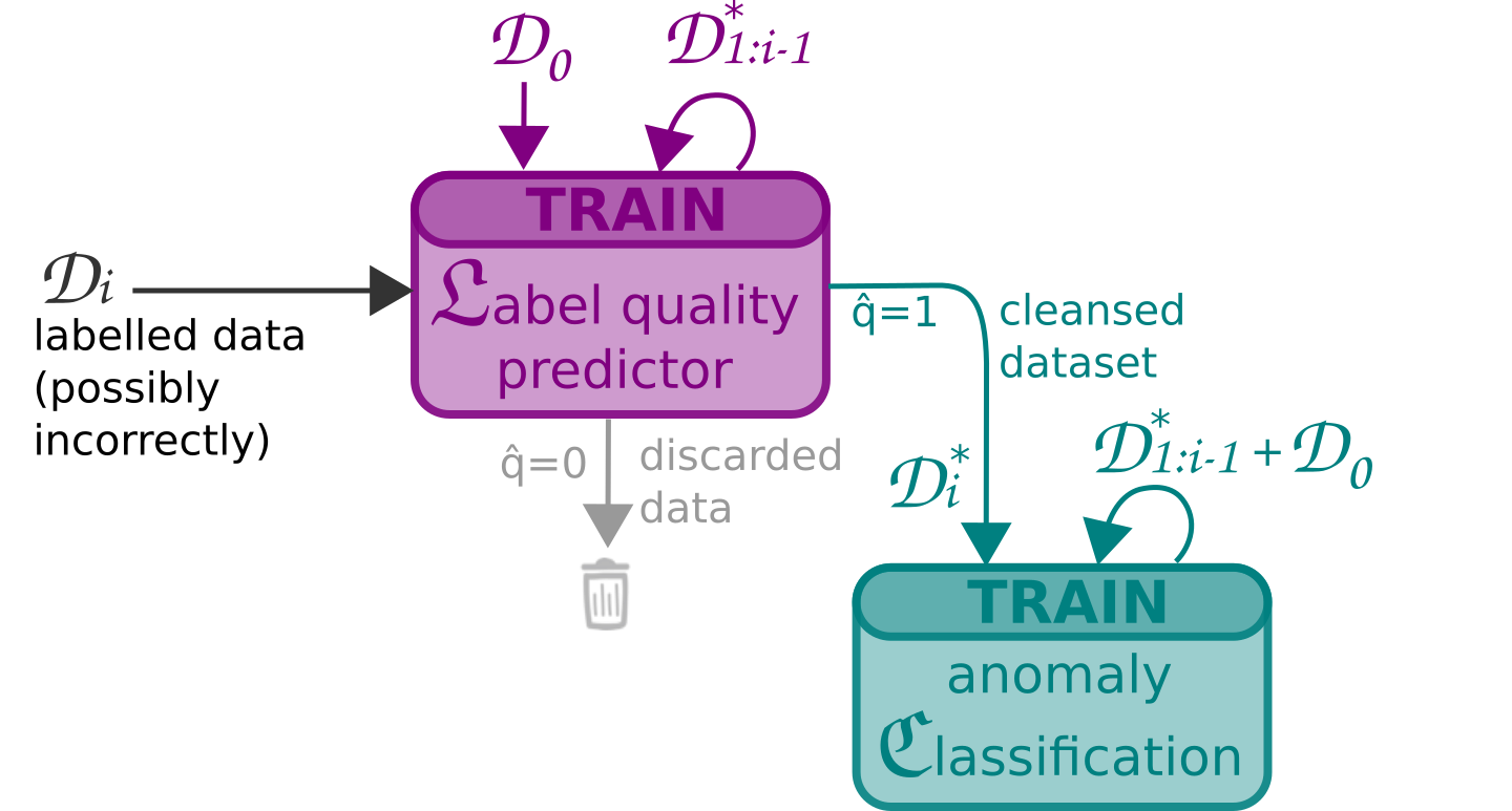
Figure 5: RAD training data selection framework. Each block is a machine learning algorithm. Data used to train is represented by colored arrows from the top. The flowchart is iterated at every batch arrival with new labelled and unlabelled data coming in (black arrows on the left). The labelled training data for $\mathfrak{C}$ is cleansed based on the label quality predicted by $\mathfrak{L}$.

Fig. 5 describes the overall architecture of RAD training data selection. it comprises two main components. A label quality model $\mathfrak{L}$ mainly aims at discerning clean labels from dirty labels and a classifier model $\mathfrak{C}$ targets the specific classification task at hand. But both models are used for the ensemble predictions, described in Sec. IV-B3.

RAD follows a generic approach since the proposed classification framework can be used with any supervised machine learning algorithm, such as SVM, KNN, random forest, nearest centroid, DNN, etc. Moreover, RAD can be applied to a large spectrum of different applications where noisy data are collected and must be cleansed before used to train the classification model. Examples are the failure detection, attack diagnosis and face recognition illustrated in Section LABEL:sec:Evaluation.

IV-B1 Data Selection Scheme

The first component of RAD aims to select clean data instances from $\mathcal{D}$ through the quality model. The objective of the label quality model is to select the most representative data instances to train a strong classifier model. It solicits data instances with clean labels, avoiding the pitfall that the classifier overfits to the noise. RAD uses supervised-learning algorithms to continuously train the label quality model from accumulated predicted clean data instances, to build a strong classifier.

We term the following selection procedure as basic, that is the default data selection scheme of RAD which requires no addition history data lookup nor involvement of human experts. $\mathfrak{L}_{i-1}$ is the label quality model that is trained with data instances received up to time $t_{i}-1$, that is $\mathcal{D}_{0}\dots\mathcal{D}_{i-1}$. Upon the arrival of a new batch of data instances $\mathcal{D}_{i}$ at time $t_{i}$, we use the currently learned label quality model $\mathfrak{L}_{i-1}$ to predict the label quality $\hat{q}$ for each data instance in $\mathcal{D}_{i}$ by comparing the given $k$ and predicted class $\hat{k}^{\mathfrak{L}_{i}}$. If they coincide, we consider the label as clean $q=1$, otherwise as dirty $q=0$. Then we build $\mathcal{D}^{*}_{i}$ as the subset of data instances from $\mathcal{D}_{i}$ with $q=1$ and discard the instances with $q=0$. This data flow is summarized in Algorithm LABEL:alg:RAD_and_extensions.

IV-B2 Generic Approach to Handle Dynamic Data

The second component of RAD is the data classifier $\mathfrak{C}$, whose input data has dynamic noise ratios. $\mathfrak{C}_{i}$ is trained on all predicted clean data instances $\mathcal{D^{*}}$ received until time $t_{i}$, that is $\mathcal{D^{*}}_{0}\dots\mathcal{D^{*}}_{i}$. We assume that $\mathcal{D}_{0}$ contains only clean data instances to kick-start the framework and use the label quality model $\mathfrak{L}_{0}\dots\mathfrak{L}_{i-1}$ to cleanse $\mathcal{D}_{1}\dots\mathcal{D}_{i}$ and produce $\mathcal{D^{*}}_{1}\dots\mathcal{D^{*}}_{i}$. Thus, the RAD framework uses the batch-by-batch updated data label quality model to enrich the training data of the classification model.

IV-B3 Prediction Techniques

Fig. 6 shows the structure of ensemble prediction, which combines the prediction outcomes of both the quality and classification models. The combined decision leverages the confidence from the output probability vectors and the test accuracy of both models from the previous training epoch. If the predictions of the two models coincide, the common prediction is used. If not, we use the prediction of the model having higher confidence. As for the confidence measure, we use the class probability from the output vector multiplied by the test accuracy of the last epoch. We provide the details in Algorithm 1.

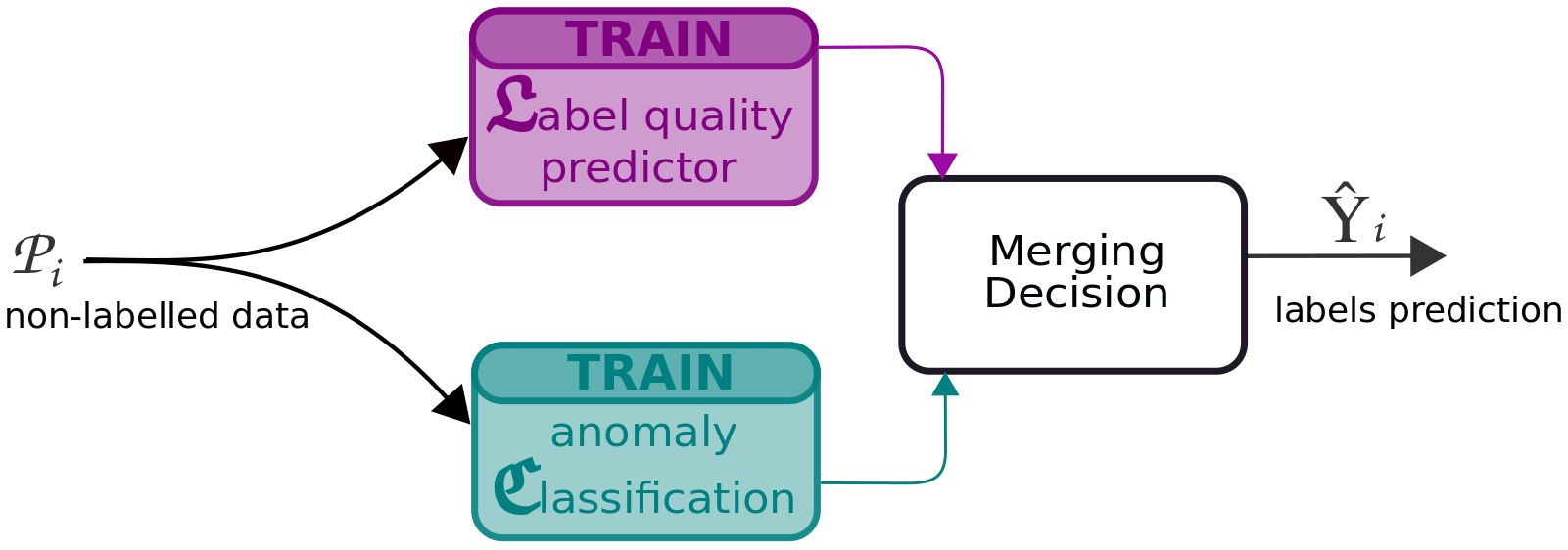
Figure 6: Ensemble Prediction.

Algorithm 1 Ensemble Prediction

Input: Test data $\mathcal{P}_{i}$, label quality model $\mathfrak{L}_{i}$, classification model $\mathfrak{C}_{i}$, testing accuracy $\alpha^{\mathfrak{L}_{i-1}}$ of $\mathfrak{L}_{i-1}$ and $\alpha^{\mathfrak{C}_{i-1}}$ of $\mathfrak{C}_{i-1}$.
Conv(): convert probability vector to class. Max(): return maximum value in a vector.
      Output: Predicted labels $\hat{Y}_{i}$

1:Get predicted labels for $\mathcal{P}_{i}$ by $\mathfrak{L}_{i}$ ($Y_{i}^{\mathfrak{L}^{\mathcal{P}}}$) and $\mathfrak{C}_{i}$ ($Y_{i}^{\mathfrak{C}^{\mathcal{P}}}$). Both have length $|\mathcal{P}_{i}|$ where each element is a vector with probabilities for each of the $K$ classes summing to 1.

2:Initialize an empty $\hat{Y}_{i}$ of length $|\mathcal{P}_{i}|$

3:for $j\in\{1,2,\dots,|\mathcal{P}_{i}|$} do

4:     if  Conv($Y_{i}^{\mathfrak{L}^{\mathcal{P}}}$[j]) = Conv($Y_{i}^{\mathfrak{C}^{\mathcal{P}}}$[j]) then

5:         $\hat{Y}_{i}$[j] $\leftarrow$ Conv($Y_{i}^{\mathfrak{C}^{\mathcal{P}}}$[j])

6:     else

7:         if $\alpha^{\mathfrak{C}_{i-1}}\times Max(Y_{i}^{\mathfrak{C}^{\mathcal{P}}}[j])>\alpha^{\mathfrak{L}_{i-1}}\times Max(Y_{i}^{\mathfrak{L}^{\mathcal{P}}}[j])$ then

8:              $\hat{Y}_{i}$[j] $\leftarrow$ Conv($Y_{i}^{\mathfrak{C}^{\mathcal{P}}}$[j])

9:         else

10:              $\hat{Y}_{i}$[j] $\leftarrow$ Conv($Y_{i}^{\mathfrak{L}^{\mathcal{P}}}$[j])

11:         end if

12:     end if

13:end for

14:return $\hat{Y}_{i}$