Graph Attention Recurrent Neural Networks for Correlated Time Series Forecasting—Full Version

Abstract

We consider a setting where multiple entities interact with each other over time and the time-varying statuses of the entities are represented as multiple correlated time series. For example, speed sensors are deployed in different locations in a road network, where the speed of a specific location across time is captured by the corresponding sensor as a time series, resulting in multiple speed time series from different locations, which are often correlated. To enable accurate forecasting on correlated time series, we proposes graph attention recurrent neural networks. First, we build a graph among different entities by taking into account spatial proximity and employ a multi-head attention mechanism to derive adaptive weight matrices for the graph to capture the correlations among vertices (e.g., speeds at different locations) at different timestamps. Second, we employ recurrent neural networks to take into account temporal dependency while taking into account the adaptive weight matrices learned from the first step to consider the correlations among time series. Experiments on a large real-world speed time series data set suggest that the proposed method is effective and outperforms the state-of-the-art in most settings. This manuscript provides a full version of a workshop paper [1].

I Introduction

Complex cyber-physical systems (CPSs) often consist of multiple entities that interact with each other across time. With the continued digitization, various sensor technologies are deployed to record time-varying attributes of such entities, thus producing correlated time series [2, 3]. One representative example of such CPSs is road transportation system [4, 5], where the speeds on different roads are captured by different sensors, such as loop detectors, speed cameras, and bluetooth speedometers, as multiple speed time series [6, 7, 8].

Accurate forecasting of correlated time series have the potential to reveal holistic system dynamics of the underlying CPSs, including predicting future behavior [2] and detecting anomalies [9, 10], which are important to enable effective operations of the CPSs. For example, in an intelligent transportation system, analyzing speed time series enables travel time forecasting, early warning of congestion, and predicting the effect of incidents, which help drivers make routing decisions [11, 12].

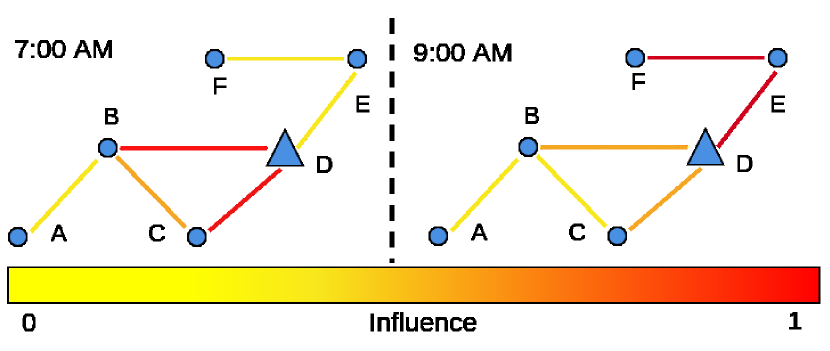
Figure 1: Dynamic Interactions

Traffic on different roads often has an impact of the neighbour roads. An accident on one road might cause congestion on the others. Most of the related work capture such interactions as a graph which is pre-computed based on different metrics such as road or euclidean distance between pairwise entities. Although such methods are easy to implement, they only capture static interactions between entities. In contrast, the interactions among entities are often dynamic and evolve across time. Figure 1 shows a graph of 6 vertices representing 6 entities, e.g., speed sensors. At 7 AM vertex $D$ has strong connections with vertices $B$ and $C$, while at 9 AM, the connections with vertices $B$ and $C$ become weaker but vertex $D$ has a stronger connection with vertex $E$ instead. However, most of the recent studies fall short on capturing such dynamics [13, 14, 15, 3].

To enable accurate and robust correlated time series forecasting, it is essential to model such spatio-temporal correlations among multiple time series. To this end, we propose graph attention recurrent neural networks (GA-RNNs).

We first build a graph among different entities by taking into account spatial proximity. In the graph, vertices represent entities and two vertices are connected by an edge if the two corresponding entities are nearby. After building the graph, we apply multi-head attention to learn an attention matrix. For each vertex, the attention matrix indicates, among all the vertex’s neighbor vertices, which neighboring vertices’ speeds are more relevant when predicting the speed of the vertex.

Next, since recurrent neural networks (RNNs) are able to well capture temporal dependency, we modify classic RNNs to capture spatio-temporal dependency. Specifically, we replace weight multiplications in classic RNNs with convolutions that take into account graph topology (e.g., graph convolution or diffusion convolution [13]). However, instead of using a static adjacency matrix, we employ the attention matrix learned from the first step to obtain adaptive adjacency matrices. Here, with the learned attention weight matrices and the inputs at different timestamps, we obtain different adjacency matrices at different timestamps, which are able to capture the dynamic correlations among different time series at different timestamps.

The main contribution is to utilize attention to derive adaptive adjacency matrices which are then utilized in RNNs to capture spatio-temporal correlations among time series to enable accurate forecasting for correlated time series. The proposed graph attention is a generic approach which can be applied to any graph-based convolution operations that utilizes adjacency matrices such as graph convolution and diffusion convolution [13]. Experiments on a large real-word traffic time series offer evidence that the proposed method is accurate and robust.

II Problem definition

We first consider the temporal aspects by introducing multiple time series and then the spatial aspects by defining graph signals. Finally, we define correlated time series forecasting.

II-A Time Series

Consider a cyber-physical system (CPS) where we have $N$ entities. The status of the $i$-th entity across time, e.g., from timestamps 1 to $T$, is represented by a time series $TS^{(i)}=\langle\mathbf{x}_{1}^{(i)},\mathbf{x}_{2}^{(i)},\ldots,\mathbf{x}_{T}^{(i)}\rangle$, where a $K$-dimensional vector $\mathbf{x}_{j}^{(i)}$ records $K$ features (e.g., speed and traffic flow) of the $i$-th entity at timestamp $j$.

Since we have a time series for each entity, we have in total $N$ time series: $TS^{(1)}$, $TS^{(2)}$, …, $TS^{(N)}$.

Given historical statuses of all entities, we aim at predicting the future statuses of all entities. More specifically, from the time series, we have historical statuses covering a window $[t_{a-L+1},t_{a}]$ that contains $L$ time stamps, and we aim at predicting the future statuses in a future window $[t_{a+1},t_{a+P}]$ that contains $P$ time stamps. We call this problem $p$-step ahead forecasting.

II-B Graph Signals

We still consider the CPS with $N$ entities. Now, we focus on the modeling of interactions among these entities.

We build a directed graph $G=(V,E)$ where each vertex $v\in V$ represents an entity in the CPS, which is often associated with spatial information such as longitude and latitude. Since we have $N$ entities in total, we have $|V|=N$. Edges are represented by adjacency matrix $E\in\mathbb{R}^{N\times N}$, where $E[i,j]=1$ represents an edge from the i-th to the j-th vertices.

If the entities are already embedded into a spatial network, e.g., camera sensors deployed in road intersections in a road network, we connect two entities by an edge if they are connected in the spatial network. Otherwise, we connect two entities by an edge if the distance between them is smaller then a threshold, which is shown to be effective [13].

At each timestamp $t$, each entity is associated with $K$ features (e.g., speed and traffic flow). We introduce a graph signal at $t$, as shown in Figure 2(a), where $\mathbf{X}_{t}\in\mathbb{R}^{N\times K}=[\mathbf{x}_{t}^{(1)},\mathbf{x}_{t}^{(2)},\ldots,\mathbf{x}_{t}^{(N)}]^{T}$ represent all features from all entities at timestamp $t$. Based on the concept of graph signals, the problem becomes learning a function that takes as input $L$ past graph signals and outputs $P$ future graph signals:

$$\mathbf{X}^{(L)}\rightarrow\mathbf{X}^{(P)},$$

where $\mathbf{X}^{(L)}=[\mathbf{X}_{(t-L+1)},\ldots,\mathbf{X}_{(t-1)},\mathbf{X}_{(t)}]$, $\mathbf{X}^{(P)}=[\mathbf{X}_{(t+1)},\mathbf{X}_{(t+2)},\ldots,\mathbf{X}_{(t+P)}]$, and $t$ is the current timestamp.

(a) Graph signal at a timestamp

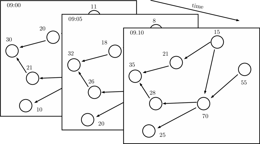
(b) Graph signals at different timestamps

Figure 2: A Time Series of Graph Signals, $K=3$.

III Graph Attention RNNs

We proceed to describe the proposed graph attention recurrent neural network (GARNN) to solve the $p$-step ahead forecasting.

III-A GARNN Framework

Figure 3: Graph Attention Recurrent Neural Network

The proposed GARNN consists of two parts, an attention part and an RNN part, which follow an encoder-decoder architecture as shown in Fig. 3. At each timestamp, we firstly model the spatial correlations among different entities using multi-head attention as two adjacency matrices $\mathbf{A}_{t}^{out}$ and $\mathbf{A}_{t}^{in}$, which consider the outgoing and incoming traffic, respectively. Next, the two attention weight matrices are fed into an RNN unit together with the input graph signal at the time stamp, which facilitate the RNN unit not only capture the temporal dependency but also the spatial correlations, making it is possible to capture the spatio-temporal correlations among different time series.

III-B Spatial Modeling

To capture the spatial correlations among different entities at a specific timestamp, we employ attention mechanism [16]. The idea is to determine, in order to predict the features of an entity, i.e., a vertex, how much should we consider the features of the vertex’s neighbour vertices. We may consider different neighbour vertices differently at different timestamps. Specifically, for each vertex $i$, we compute an attention score w.r.t. to each vertex in $NB(i)=\{j|E[i,j]=1\}\cup\{i\}$, i.e., vertex $i$’s neighbour vertices and itself.

We proceed to show how to compute an attention score for vertex $i$. Recall that for any vertex $i$ in the graph, its features at timestamp $t$ is represented by a $K$-dimensional vector $\mathbf{x}_{t}^{(i)}\in\mathbb{R}^{K}$. Vertex $j$ is a vertex from $NB(i)$. Attention score $\mathbf{A}_{t}[i,j]$ indicates how much attention should be paid to vertex $j$’s features in order to estimate vertex $i$’s features at timestamp $t$, which is computed based on Equation 1, where $[\cdot||\cdot]$ represents the concatenation operator.

$$\small A_{t}[i,j]=\frac{exp(LReLU(\mathbf{v}^{\intercal}[\mathbf{W}\mathbf{x}_{t}^{(i)}\;||\;\mathbf{W}\mathbf{x}_{t}^{(j)}]))}{\sum_{m\in NB(i)}exp(LReLU(\mathbf{v}^{\intercal}[\mathbf{W}\mathbf{x}_{t}^{(i)}\;||\;\mathbf{W}\mathbf{x}_{t}^{(m)}]))}$$ (1)

First, we embed the features from each vertex with an embedding matrix $\mathbf{W}\in\mathcal{R}^{F\times K}$, where $F$ is the size of the embedding. Then, we concatenate the embeddings of the two vertices’ features $\mathbf{Wx}_{t}^{(i)}$ and $\mathbf{Wx}_{t}^{(j)}$, which is fed into an attention network. The attention network is constructed as a single-layer feed forward neural network, parameterized by a weight matrix $\mathbf{v}\in\mathbb{R}^{2\cdot F\times 1}$. In addition, we apply a LeakyReLU function $\mathit{LReLU}$ with a negative input slope of $a=0.2$ as activation function (see Euqation  2). Finally, we apply softmax to normalize the final output to obtain $\mathbf{A}_{t}[i,j]$ so that the results are easier to interpret.

$$\mathit{LReLU}(x)=\begin{dcases}ax,&\text{if }x\leq 0\\ x,&\text{if }x\;\textgreater\;0\end{dcases}$$ (2)

Motivated by [17], we observe that stacking multiple attention networks, a.k.a., attention heads, is beneficial since each attention network can specialise on capturing different interactions. Assume that we use a total of $C$ attention networks, each network has its own embedding matrix $\mathbf{W}^{(c)}\in\mathcal{R}^{F\times K}$ and weight matrix $\mathbf{v}^{(c)}\in\mathbb{R}^{2\cdot F\times 1}$ in the feed forward neural network. There are multiple ways of combining the attention heads, in our experiments we use average according to Equation 3,

$$\small\mathbf{A}_{t}[i,j]=\frac{1}{C}\sum_{c=1}^{C}\frac{exp(LReLU(\mathbf{v}_{c}^{\intercal}[\mathbf{W}_{c}\mathbf{x}_{t}^{(i)}\;||\;\mathbf{W}_{c}\mathbf{x}_{t}^{(j)}]))}{\sum_{m\in NB(i)}exp(LReLU(v_{c}^{\intercal}[\mathbf{W}_{c}\mathbf{x}_{t}^{(i)}\;||\;\mathbf{W}_{c}\mathbf{x}_{t}^{(j)}]))}$$ (3)

So far, for each vertex, we have computed the attentions to all its neighbors, which captures the influence of the outgoing traffic. On the other hand, it is also of interest to capture the influence of the incoming traffic. To this end, we use the transpose of the adjacency matrix $E$ to define neighboring vertices and apply the same attention mechanism to obtain another attention matrix to represent the influence of incoming traffic. Finally, we obtain two attention matrices $\mathbf{A}_{t}^{out}\in\mathbb{R}^{N\times N}$ and $\mathbf{A}_{t}^{in}\in\mathbb{R}^{N\times N}$, which capture the influence from outgoing traffic and incoming traffic, respectively.

III-C Spatio-Temporal Modeling

We integrate the learned attention matrices into classical recurrent neural networks to capture spatio-temporal correlations. We follow an encoder-decoder architecture as shown in Figure 3, which is able to well capture the temporal dependencies across time. Next, we replace the matrix multiplications in RNN units by convolutions that take into account graph topology such as diffusion convolution or graph convolution. Here, instead of using a static adjacency matrix $E$ that only captures connectivity, the convolution here employs the learned adjacency matrices $\mathbf{A}_{t}^{out}$ and $\mathbf{A}_{t}^{out}$ at timestamp $t$. Note that although the attention embedding and weight matrices $\mathbf{W}_{c}$ and $\mathbf{v}_{c}$ are static across time, the input matrices $\mathbf{x}_{t}^{(i)}$ are changing across time. Thus, we are able to derive different adjacency matrices $\mathbf{A}_{t}^{out}$ and $\mathbf{A}_{t}^{out}$ at different timestamps.

More specifically, we proceed to define a diffusion convolution operator $\otimes$ on a graph signal $\mathbf{X}_{t}\in\mathcal{R}^{N\times K}$ using the learned attention matrices $\mathbf{A}_{t}^{out}$ and $\mathbf{A}_{t}^{in}$ at timestamp $t$ in Equation 4.

$$\small\begin{split}X_{t}\otimes\Theta=\alpha(\sum_{k=1}^{K}\sum_{h=1}^{H}(\theta_{k,h,1}(\mathbf{A}_{t}^{out})^{h}+&\theta_{k,h,2}(\mathbf{A}_{t}^{in})^{h})\mathbf{X}_{t}[\cdot,k])\end{split}$$ (4)

Here, $\alpha$ is an activation function, matrix $\Theta\in\mathcal{R}^{K\times H\times 2}$ is a filter to be learned, and $\mathbf{X}_{t}[\cdot,k]$ represents the $k$-th column of graph signal $\mathbf{X}_{t}$, which is the $k$-th features of all entities. We often apply $Q$ different filters to perform diffusion convolutions and then concatenate the results into a matrix $\mathbf{X}_{t}\otimes\mathbf{\Theta}=[\mathbf{X}_{t}\otimes\Theta_{1}||\mathbf{X}_{t}\otimes\Theta_{2}||\ldots||\mathbf{X}_{t}\otimes\Theta_{Q}]$. Finally, graph signal $\mathbf{X}_{t}$ is convoluted into matrix $\mathbf{X}_{t}\otimes\mathbf{\Theta}\in\mathcal{R}^{N\times Q}$.

Next, we integrate the proposed graph attention based convolution into an RNN. Here, we use a Gated Recurrent Unit (GRU) [18] as an RNN unit to illustrate the integration, where the matrix multiplications in classic GRU are replaced by the graph attention based diffusion convolutional process as defined in Equation 4.

$$r_{t} =\sigma(\mathbf{\Theta}_{r}\otimes[\mathbf{X}_{t}||\mathbf{H}_{t-1}]+b_{r})$$

$$u_{t} =\sigma(\mathbf{\Theta}_{u}\otimes[\mathbf{X}_{t}||\mathbf{H}_{t-1}]+b_{u})$$

$$\hat{h}_{t} =tanh(\mathbf{\Theta}_{\hat{h}}\otimes[\mathbf{X}_{t}||(r_{t}\odot\mathbf{H}_{t-1})]+b_{\hat{h}})$$

$$\mathbf{H}_{t} =u_{t}\odot\mathbf{H}_{t-1}+(1-u_{t})\odot\hat{h}_{t}$$

Here, $\mathbf{X}_{t}\in\mathcal{R}^{N\times K}$ is the graph signal at timestamp $t$, $\mathbf{H}_{t}$ is the output at timestamp $t$. $r_{t}$, $u_{t}$ and $\hat{h}_{t}$ represent the reset gate, update gate, and candidate context at time $t$. $\otimes$ indicates the proposed graph attention based diffusion convolution, and $\mathbf{\Theta}_{r}$, $\mathbf{\Theta}_{u}$, and $\mathbf{\Theta}_{\hat{h}}$ are the filters used in the three convolutions. $\odot$ is Hadamard product.

The proposed graph attention is generic in the sense that it provides a data-driven manner to produce dynamic adjacency matrices and thus can be integrated with different kinds of convolutions that utilize graph adjacency matrices. Such convolutions often use a static adjacency matrix, while the proposed graph attention allows us to employ dynamic adjacency matrices at different timestamps, which are expected to better capture the spatio-temporal correlations among different time series.

III-D Loss Function

The loss function measures the discrepancy between the estimated travel speed and the ground truth at each timestamp for each entity. Suppose that we have $Y$ training instances in total, we use Equation 5 to measure the discrepancy.

$$\mathit{loss}=\frac{1}{YNP}\sum_{y=1}^{Y}\sum_{n=1}^{N}\sum_{p=1}^{P}|\mathbf{x}_{p,y}^{(n)}-\mathbf{\hat{x}}_{p,y}^{(n)}|$$ (5)

where $\mathbf{x}_{p,y}^{(n)}$ and $\mathbf{\hat{x}}_{p,y}^{(n)}$ are the ground truth and the estimated speed for the $n$-th entity at timestamp $p$ in the $y$-th training instance.

IV Empirical Study

Data	Models	15 min			30 min			60 min
		MAE	RMSE	MAPE	MAE	RMSE	MAPE	MAE	RMSE	MAPE
METR-LA	HA	4.16	7.80	13.0%	4.16	7.80	13.0%	4.16	7.80	13.0%
	ARIMA	3.99	8.21	9.6%	5.15	10.45	12.7%	6.90	13.23	17.4%
	VAR	4.42	7.89	10.2%	5.41	9.13	12.7%	6.52	10.11	15.8%
	SVR	3.99	8.45	9.3%	5.05	10.87	12.1%	6.72	13.76	16.7%
	FC-LSTM	3.44	6.30	9.6%	3.77	7.23	10.9%	4.37	8.69	13.2%
	WaveNet	2.99	5.89	8.0%	3.59	7.28	10.2%	4.45	8.93	13.6%
	STGCN	2.88	5.74	7.6%	3.47	7.24	9.5%	4.59	9.40	12.7%
	GCRNN	2.80	5.51	7.5%	3.24	6.74	9.0%	3.70	8.16	10.9%
	GA-GCRNN	2.76	5.33	7.1%	3.21	6.45	8.8%	3.70	7.68	10.9%
	DCRNN	2.77	5.38	7.3%	3.15	6.45	8.8%	3.60	7.60	10.5%
	GA-DCRNN	2.75	5.28	7.0%	3.14	6.39	8.0%	3.72	7.64	11.0%

TABLE I: Accuracy at $p=3$, $p=6$, and $p=12$

IV-A Experimental Setup

We conducted experiments on a large real world traffic dataset METR-LA from [13]. The dataset consists of speed measurements from 207 loop detectors spread across Los Angeles highways. The data was collected between March 1st 2012 and June 30th 2012 with a frequency of every 5 minutes.

We follow the same experimental setup as [13]. We build a graph by connecting from sensors $i$ to $j$ if the road network distance from $i$ to $j$ is small [13]. Since road network distance is used, the distance from $i$ to $j$ may be different from the distance from $j$ to $i$, making the adjacency matrix $E$ asymmetric. We use 70% of the data for training, 10% for validation and 20% for testing. We consider three metrics to evaluate the prediction accuracy: Mean Absolute Error (MAE), Root Mean Square Error (RMSE), Mean Absolute Percentage Error (MAPE). We consider the same forecasting setting as [13] where we use $l=12$ past observations to predict the next $p=12$ steps ahead and report the errors at three different intervals (15, 30, and 60 mins) and also the average errors over $p=12$ steps.

IV-B Implementation Details

The method is implemented in Python 3.6 using Tensorflow 1.7. A server with Intel Xeon Platinum 8168 CPU and 2 Tesla V100 GPUS are used to conduct all experiments. We trained the model using Adam optimizer with 0.01 as learning rate which decreases every 10 epochs after the 40th iteration. We used a total of $C=2$ attention heads with an embedding size of $F=16$. In addition we used a 2 layer GRU, with 64 units, a batch size of 64, and the scheduled sampling technique as described in [13].

IV-C Experimental Results

Baselines: We compared our proposed model with the following methods:

• HA historical average [13]. HA models the data as a seasonal process and computes the predictions as a weighted average of the previous seasons.

• ARIMA [arima] integrated moving average model with Kalman filter which is widely used for time series forecasting.

• VAR [19] vector auto-regression.

• SVR support vector regression.

• FC-LSTM [20] recurrent neural network with fully connected LSTM units.

• WaveNet [21] a dilated causal convolution network.

• STGCN [14] spatial-temporal GCN that combines 1D convolution with graph convolution.

• GCRNN [13] graph convolutional recurrent neural network.

• DCRNN [13] diffusion convolutional recurrent neural network.

A more in-dept description of the baselines, along with hyper-parameters can be found in [13]. Since GCRNN and DCRNN employ graph based convolutions, where GCRNN uses graph convolution and DCRNN uses diffusion convolution [13], we incorporate the proposed graph attention based adaptive adjacency matrix into the two methods to obtain GA-GCRNN and GA-DCRNN.

Accuracy: We compare the proposed GA-GCRNN and GA-DCRNN with the baselines in Table I. Firstly, we observe that non-deep learning methods such as ARIMA, VAR and SVR perform poorly compared to the deep learning methods especially when $p$ is large. This is because the temporal dependencies becomes increasingly non-linear as the horizon increases and the aforementioned baselines are unable to capture such dynamics.

We also observe that by considering the underlying correlations among entities using a graph is very effective on improving the accuracy. Here, FC-LSTM and WaveNet do not consider such correlations and are outperformed by the other deep learning methods that consider the correlations.

Next, we evaluate the proposed graph attention method for generating the dynamic adjacency matrices. We first compare GA-GCRNN with GCRNN, where GA-GCRNN outperforms GCRNN in all settings (see the underline values in Table I). We then consider GA-DCRNN. GA-DCRNN outperforms DCRNN in most settings (see the bold values in Table I), especially in short term predictions at 15 and 30 minutes.

We also consider the average accuracy over all the 12 steps in the prediction, as shown in Table II. On average, GA-DCRNN is better when using RMSE and MAPE. This suggests that GA-DCRNN avoids having large prediction errors but may have more small prediction errors than does DCRNN. This shows that GA-DCRNN better captures the general trend of the underlying traffic data.

Models	Average
	MAE	RMSE	MAPE
GCRNN	3.28	6.80	9.13%
GA-GCRNN	3.22	6.48	8.93%
DCRNN	3.17	6.47	8.86%
GA-DCRNN	3.22	6.43	8.66%

TABLE II: Average Accuracy

The proposed graph attention based method for generating dynamic adjacency matrices is effective, which helps improve prediction accuracy, especially for short term prediction. In addition, the proposed method is generic as it can be used to boost the accuracy of both DCRNN and GCRNN.

Efficiency: While DCRNN takes on average 271 seconds for one epoch, GA-DCRNN requires 401 seconds. The discrepancy between the two models is due to the attention mechanism, which requires more computation. Note that when implementing the attention we followed [22], but a more efficient way is available [23]. For the same reason, GA-GCRNN also takes longer time than GCRNN does.

Summary: The results suggest that the proposed graph head attention based adaptive adjacency matrices can be easily integrated with convolutions that consider graph topology and has a great potential to enable more accurate predictions, especially for relatively short term predictions. It is of interest to further investigate how to improve long term predictions.

V Related work

For time series forcasting, auto-regressive models, e.g., ARIMA, is widely used as a baseline method. Hidden Markov models are also often used to enable time series forecasting. A so-called spatio-temporal HMM (STHMM) is able to consider spatio-temporal correlations among traffic time series from adjacent edges [3].

Neural networks are able to capture non-linear dependencies within the data, which enable non-linear forecasting models and this category of models started to receive greater attention in the last years. In particular, Recurrent Neural Networks (RNNs) are used with successes in multiple domains such as traffic time series prediction [13] or wind forecasting [24], due to their recurrent nature that is able to capture temporal relationships within the data. However they suffer from the well known vanishing gradient problem [25]. Different models such as Long-Short-Term-Memory (LSTM) or Gated-Recurrent-Unit (GRU) come as an extension to traditional RNNs. The core idea of RNN models is by integrating different gates to control what the network is going to learn and forget leading to better results and an elegant solution for the vanishing problem.

Another well known type of deep learning models are Convolutions Neural Networks (CNNs). CNNs are considered to be the state of the art when it comes to speech or image recognition. CNN based models are well known for their ability to capture spatial relationships, nearby elements, e.g., pixels in images, share local features by traversing the input multiple times and applying different filters. CNNs often work on grid-based inputs, limiting its applicability to graph-based inputs such as road networks. Recently, Bruna et al. [26] introduce Graph Convolutional Networks (GCNs) that combines spectral graphs theory with CNNs. Two recent studies employ GCNs to fill in missing values for uncertain traffic time series [27, 28]. [29] proposes Diffusion Convolution Neural Networks (DCNNs) which fall under the non-spectral methods. DCNN works on the assumption that the further two nodes are in terms of graph topology, the lower impact they should have.

DCRNN [13] extends DCNN with RNN so that it also captures time dependencies within the data. Our work is closely related and builds on top of DCRNN. The main difference is that DCRNN assumes that the adjacency matrix used in random walks is static. However, this assumption might not always hold and we propose to learn an adaptive adjacency matrix at each time stamp using attention mechanism that considers graph topology. Multi-task learning [30] has also been applied for correlated time series forecasting, where both a CNN and a RNN are combined to both forecast future values and reconstruct historical values [2]. Our work resembles [22] and [31]. The main difference is that our model tries to learn a dynamic adjacency matrix which can afterwards be used with any type of graph-RNN like structure to update each node embedding by taking into account its neighbours offering more flexibility.

From application perspectives, many smart transportation applications [32, 33, 34, 35, 36, 37] rely on accurate travel speed estimation, which can benefit from our work.

VI Conclusion and Outlook

We propose a generic method to obtain dynamic adjacency matrices using graph attention which can be integrated seamlessly with existing graph based convolutions such as graph convolution and diffusion convolution. More specifically, we show how the integration of adaptive adjacency matrices and recurrent neural networks is able to improve the correlated time series predictions where the relationships among different time series can be captured as a graph. Experimental results show great potential when using adaptive adjacency matrices, especially for short term predictions.

As future work, it is of interest to explore how speed up the attention computation using, e.g., parallel computation [38]. It is also of interest to explore how to incorporate additional knowledge of the entities, e.g., points of interest around the speed sensors.

References

- [1] R.-G. Cirstea, B. Yang, and C. Guo, “Graph attention recurrent neural networks for correlated time series forecasting.” in MileTS19@KDD, 2019.
- [2] R. Cirstea, D. Micu, G. Muresan, C. Guo, and B. Yang, “Correlated time series forecasting using multi-task deep neural networks,” in CIKM, 2018, pp. 1527–1530.
- [3] B. Yang, C. Guo, and C. S. Jensen, “Travel cost inference from sparse, spatio-temporally correlated time series using markov models,” PVLDB, vol. 6, no. 9, pp. 769–780, 2013.
- [4] B. Yang, J. Dai, C. Guo, C. S. Jensen, and J. Hu, “PACE: a path-centric paradigm for stochastic path finding,” VLDB J., vol. 27, no. 2, pp. 153–178, 2018.
- [5] Z. Ding, B. Yang, Y. Chi, and L. Guo, “Enabling smart transportation systems: A parallel spatio-temporal database approach,” IEEE Trans. Computers, vol. 65, no. 5, pp. 1377–1391, 2016.
- [6] J. Hu, B. Yang, C. Guo, and C. S. Jensen, “Risk-aware path selection with time-varying, uncertain travel costs: a time series approach,” VLDB J., vol. 27, no. 2, pp. 179–200, 2018.
- [7] C. Guo, C. S. Jensen, and B. Yang, “Towards total traffic awareness,” SIGMOD Record, vol. 43, no. 3, pp. 18–23, 2014.
- [8] J. Hu, B. Yang, C. S. Jensen, and Y. Ma, “Enabling time-dependent uncertain eco-weights for road networks,” GeoInformatica, vol. 21, no. 1, pp. 57–88, 2017.
- [9] T. Kieu, B. Yang, and C. S. Jensen, “Outlier detection for multidimensional time series using deep neural networks,” in MDM, 2018, pp. 125–134.
- [10] T. Kieu, B. Yang, C. Guo, and C. S. Jensen, “Outlier detection for time series with recurrent autoencoder ensembles,” in IJCAI, 2019.
- [11] H. Liu, C. Jin, B. Yang, and A. Zhou, “Finding top-k shortest paths with diversity,” IEEE Trans. Knowl. Data Eng., vol. 30, no. 3, pp. 488–502, 2018.
- [12] C. Guo, B. Yang, J. Hu, and C. S. Jensen, “Learning to route with sparse trajectory sets,” in ICDE, 2018, pp. 1073–1084.
- [13] Y. Li, R. Yu, C. Shahabi, and Y. Liu, “Diffusion convolutional recurrent neural network: Data-driven traffic forecasting,” in ICLR, 2018.
- [14] B. Yu, H. Yin, and Z. Zhu, “Spatio-temporal graph convolutional networks: A deep learning framework for traffic forecasting,” arXiv preprint arXiv:1709.04875, 2017.
- [15] C. Chen, K. Li, S. G. Teo, X. Zou, K. Wang, J. Wang, and Z. Zeng, “Gated residual recurrent graph neural networks for traffic prediction,” in Proceedings of the AAAI Conference on Artificial Intelligence, vol. 33, 2019, pp. 485–492.
- [16] D. Bahdanau, K. Cho, and Y. Bengio, “Neural machine translation by jointly learning to align and translate,” arXiv preprint arXiv:1409.0473, 2014.
- [17] A. Vaswani, N. Shazeer, N. Parmar, J. Uszkoreit, L. Jones, A. N. Gomez, L. Kaiser, and I. Polosukhin, “Attention is all you need,” CoRR, vol. abs/1706.03762, 2017.
- [18] J. Chung, Ç. Gülçehre, K. Cho, and Y. Bengio, “Empirical evaluation of gated recurrent neural networks on sequence modeling,” CoRR, vol. abs/1412.3555, 2014. [Online]. Available: http://arxiv.org/abs/1412.3555
- [19] J. D. Hamilton, Time series analysis. Princeton New Jersey, 1994, vol. 2.
- [20] I. Sutskever, O. Vinyals, and Q. V. Le, “Sequence to sequence learning with neural networks,” in Advances in neural information processing systems, 2014, pp. 3104–3112.
- [21] A. v. d. Oord, S. Dieleman, H. Zen, K. Simonyan, O. Vinyals, A. Graves, N. Kalchbrenner, A. Senior, and K. Kavukcuoglu, “Wavenet: A generative model for raw audio,” arXiv preprint arXiv:1609.03499, 2016.
- [22] P. Veličković, G. Cucurull, A. Casanova, A. Romero, P. Lio, and Y. Bengio, “Graph attention networks,” arXiv preprint arXiv:1710.10903, 2017.
- [23] Z. Liu, C. Chen, L. Li, J. Zhou, X. Li, L. Song, and Y. Qi, “Geniepath: Graph neural networks with adaptive receptive paths,” arXiv preprint arXiv:1802.00910, 2018.
- [24] A. Yadav and K. Sahu, “Wind forecasting using artificial neural networks: a survey and taxonomy,” International Journal of Research In Science & Engineering, vol. 3, 2017.
- [25] S. Hochreiter, Y. Bengio, P. Frasconi, J. Schmidhuber et al., “Gradient flow in recurrent nets: the difficulty of learning long-term dependencies.(2001),” Cited on, p. 114, 2001.
- [26] J. Bruna, W. Zaremba, A. Szlam, and Y. LeCun, “Spectral networks and locally connected networks on graphs,” CoRR, vol. abs/1312.6203, 2013. [Online]. Available: http://arxiv.org/abs/1312.6203
- [27] J. Hu, C. Guo, B. Yang, and C. S. Jensen, “Stochastic weight completion for road networks using graph convolutional networks,” in ICDE, 2019, pp. 1274–1285.
- [28] J. Hu, C. Guo, B. Yang, C. S. Jensen, and H. Xiong, “Stochastic origin-destination matrix forecasting using dual-stage graph convolutional, recurrent neural networks,” in ICDE, 2020, pp. 1417–1428.
- [29] J. Atwood and D. Towsley, “Search-convolutional neural networks,” CoRR, vol. abs/1511.02136, 2015. [Online]. Available: http://arxiv.org/abs/1511.02136
- [30] T. Kieu, B. Yang, C. Guo, and C. S. Jensen, “Distinguishing trajectories from different drivers using incompletely labeled trajectories,” in CIKM, 2018, pp. 863–872.
- [31] J. Zhang, X. Shi, J. Xie, H. Ma, I. King, and D.-Y. Yeung, “Gaan: Gated attention networks for learning on large and spatiotemporal graphs,” arXiv preprint arXiv:1803.07294, 2018.
- [32] S. A. Pedersen, B. Yang, and C. S. Jensen, “A hybrid learning approach to stochastic routing,” in ICDE, 2020, pp. 2010–2013.
- [33] C. Guo, B. Yang, J. Hu, C. S. Jensen, and L. Chen, “Context-aware, preference-based vehicle routing.” VLDB Journal, online first, 2020.
- [34] S. B. Yang and B. Yang, “Learning to rank paths in spatial networks,” in ICDE, 2020, pp. 2006–2009.
- [35] S. A. Pedersen, B. Yang, and C. S. Jensen, “Anytime stochastic routing with hybrid learning,” Proc. VLDB Endow., vol. 13, no. 9, pp. 1555–1567, 2020.
- [36] S. Aljubayrin, B. Yang, C. S. Jensen, and R. Zhang, “Finding non-dominated paths in uncertain road networks,” in SIGSPATIAL, 2016, pp. 15:1–15:10.
- [37] S. A. Pedersen, B. Yang, and C. S. Jensen, “Fast stochastic routing under time-varying uncertainty,” VLDB J., vol. 29, no. 4, pp. 819–839, 2020.
- [38] P. Yuan, C. Sha, X. Wang, B. Yang, A. Zhou, and S. Yang, “XML structural similarity search using mapreduce,” in WAIM, 2010, pp. 169–181.