Acoustic word embeddings for zero-resource languages using self-supervised contrastive learning and multilingual adaptation

Abstract

Acoustic word embeddings (AWEs) are fixed-dimensional representations of variable-length speech segments. For zero-resource languages where labelled data is not available, one AWE approach is to use unsupervised autoencoder-based recurrent models. Another recent approach is to use multilingual transfer: a supervised AWE model is trained on several well-resourced languages and then applied to an unseen zero-resource language. We consider how a recent contrastive learning loss can be used in both the purely unsupervised and multilingual transfer settings. Firstly, we show that terms from an unsupervised term discovery system can be used for contrastive self-supervision, resulting in improvements over previous unsupervised monolingual AWE models. Secondly, we consider how multilingual AWE models can be adapted to a specific zero-resource language using discovered terms. We find that self-supervised contrastive adaptation outperforms adapted multilingual correspondence autoencoder and Siamese AWE models, giving the best overall results in a word discrimination task on six zero-resource languages.

Index Terms—  Acoustic word embeddings, unsupervised speech processing, transfer learning, self-supervised learning.

1 Introduction

A zero-resource language is one for which no transcribed speech resources are available for developing speech systems [1, 2]. Although conventional speech recognition is not possible for such languages, researchers have shown how speech search [3, 4, 5], discovery [6, 7, 8, 9], and segmentation and clustering [10, 11, 12] applications can be developed without any labelled speech audio. In many of these applications, a metric is required for comparing speech segments of different durations. This is typically done using dynamic time warping (DTW). But DTW is computationally expensive and can be difficult to incorporate directly into downstream systems (see e.g. the alterations required in [13]). Acoustic word embeddings (AWEs) have emerged as an alternative. Instead of using alignment, speech segments are mapped to vectors in a fixed-dimensional space. Proximity in this embedding space should indicate similarity of the original acoustic segments [14].

Several AWE models have been proposed [15, 16, 17, 18, 19, 20, 21, 22, 23, 24, 25, 26]. For zero-resource settings, one approach is to train an unsupervised model on unlabelled data from the target language. Chung et al. [27] trained an autoencoding encoder-decoder recurrent neural network (RNN) on unlabelled speech segments and used (a projection of) the final encoder hidden state as embedding. Kamper [28] extended this approach: instead of reconstructing an input segment directly, the correspondence autoencoder RNN (CAE-RNN) attempts to reconstruct another speech segment of the same type as the input. Since labelled data isn’t available for zero-resource languages, the input-output pairs for the CAE-RNN are obtained from an unsupervised term discovery (UTD) system, which automatically finds recurring word-like patterns in an unlabelled speech collection [6, 7].

A recent alternative for obtaining embeddings on a zero-resource language is to use multilingual transfer learning [29, 30, 31, 32]. The idea is to train a supervised multilingual AWE model jointly on a number of well-resourced languages for which labelled data is available, but to then apply the model to an unseen zero-resource language. This multilingual transfer approach was found to outperform monolingual unsupervised learning approaches in [31, 32].

One question is whether unsupervised learning and multilingual transfer are complementary. More concretely, can multilingual transfer further benefit from incorporating unsupervised learning? In this paper we answer this question by using unsupervised adaptation: a multilingual AWE model is updated by fine-tuning (a subset of) its parameters to a particular zero-resource language. To obtain training targets, we use the same approach as for the unsupervised model in [28], and apply a UTD system to unlabelled data from the target language. We consider unsupervised adaptation of multilingual CAE-RNN models, SiameseRNN models [33], and a new AWE approach based on self-supervised contrastive learning.

Self-supervised learning involves using proxy tasks for which target labels can automatically be obtained from the data [34, 35]. Originally proposed for vision problems [36, 37, 38], it has since also been used as an effective pretraining step for supervised speech recognition [39, 40, 41, 42, 43, 44]. It is somewhat difficult to distinguish self-supervised from unsupervised learning. But, importantly for us, a number of loss functions have been introduced in the context of self-supervised learning which have not been considered for AWEs. Here we specifically consider the contrastive loss of [46, 47]. While a Siamese AWE model [48, 33] optimises the relative distance between one positive and one negative pair, our contrastive AWE model jointly embeds a number of speech segments and then attempts to select a positive item from among several negative items. We compare the ContrastiveRNN to CAE-RNN and SiameseRNN models in both the purely unsupervised monolingual and the supervised multilingual transfer settings. We use an intrinsic word discrimination task on six languages (which we treat as zero-resource).

Our main contributions are as follows. (i) For purely unsupervised monolingual AWEs, we show that a ContrastiveRNN using UTD segments as training targets outperforms previous unsupervised models by between 5% and 19% absolute in average precision (AP). (ii) We compare contrastive learning to other supervised AWE models for multilingual transfer (without adaptation) and find that the multilingual ContrastiveRNN only gives improvements on some (but not all) zero-resource languages compared to the multilingual CAE-RNN and SiameseRNN. (iii) However, when performing unsupervised adaptation, adapted multilingual ContrastiveRNNs outperform the other adapted models on five out of six zero-resource languages, with improvements of up to 12% absolute in AP on some languages, resulting in the best reported results on these data sets. (iv) We perform probing experiments which show that the ContrastiveRNN is generally better at abstracting away from speaker identity.

2 Acoustic word embedding models

We first provide an overview of two existing acoustic word embedding (AWE) models. We then introduce a new contrastive model. Each of these models can be trained using labelled word segments (making them supervised) or by using discovered words from a UTD system (making them unsupervised); in this section we are agnostic to the training method, but we discuss how we use the different models in detail in Section 3.

2.1 Correspondence autoencoder RNN

The correspondence autoencoder recurrent neural network (CAE-RNN) [28] is an extension of an autoencoder RNN [27]. Both models consist of an encoder RNN and a decoder RNN. The encoder produces a fixed-dimensional representation of a variable-length word segment which is then fed to the input of the decoder to reconstruct the original input sequence. In the CAE-RNN, unlike the autoencoder, the target output is not identical to the input, but rather an instance of the same word type. Figure 1 illustrates this model. Formally, the CAE-RNN is trained on pairs of speech segments $(X,X^{\prime})$, with $X=\mathbf{x}_{1},\ldots,\mathbf{x}_{T}$ and $X^{\prime}=\mathbf{x}^{\prime}_{1},\ldots,\mathbf{x}^{\prime}_{T}$, containing different instances of the same word type, with each $\mathbf{x}_{t}$ an acoustic feature vector. The loss for a single training pair is therefore $J=\sum_{t=1}^{T^{\prime}}\lVert\mathbf{x}_{t}^{\prime}-\boldsymbol{f}_{t}(X)\rVert^{2}$, where $\boldsymbol{f}_{t}(X)$ is the $t^{th}$ decoder output conditioned on the embedding $\mathbf{z}$. The embedding $\mathbf{z}$ is a projection of the final encoder RNN hidden state. As in [28], we first pretrain the CAE-RNN as an autoencoder and then switch to the loss function for correspondence training.

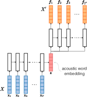
Fig. 1: The CAE-RNN is trained to reconstruct an instance $X^{\prime}$ of the same word type as the input sequence $X$. $T^{\prime}$ and $T$ are the lengths of $X^{\prime}$ and $X$, respectively.

2.2 Siamese RNN

Unlike the reconstruction loss used in the CAE-RNN, the SiameseRNN model explicitly optimises relative distances between embeddings [33]. Given input sequences $X_{a}$, $X_{p}$, $X_{n}$, the model produces embeddings $\mathbf{z}_{a}$, $\mathbf{z}_{p}$, $\mathbf{z}_{n}$, as illustrated in Figure 2. Inputs $X_{a}$ and $X_{p}$ are from the same word type (subscripts indicate anchor and positive) and $X_{n}$ is from a different word type (negative). For a single triplet of inputs, the model is trained using the triplet loss function, defined as [50, 51]: $J=\text{max}\{0,m+d(\mathbf{z}_{a},\mathbf{z}_{p})-d(\mathbf{z}_{a},\mathbf{z}_{n})\}$, with $m$ a margin parameter and $d(\mathbf{u},\mathbf{v})=1-\mathbf{u}^{\top}\mathbf{v}/\lVert\mathbf{u}\rVert\lVert\mathbf{v}\rVert$ denoting the cosine distance between two vectors $\mathbf{u}$ and $\mathbf{v}$. This loss is at a minimum when all embedding pairs $(\mathbf{z}_{a},\mathbf{z}_{p})$ of the same type are more similar by a margin $m$ than pairs $(\mathbf{z}_{a},\mathbf{z}_{n})$ of different types. To sample negative examples we use an online batch hard strategy [52]: for each item (anchor) in the batch we select the hardest positive and hardest negative example.

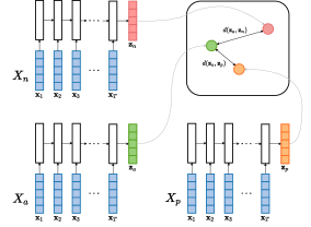
Fig. 2: In the SiameseRNN, three encoder RNNs use the same set of parameters to produce embeddings $\mathbf{z}_{a}$, $\mathbf{z}_{p}$, $\mathbf{z}_{n}$ from input segments $X_{a}$, $X_{p}$, $X_{n}$. The model is trained to minimise the distance between the anchor and the positive item while maximising the distance between the anchor and negative item.

2.3 Contrastive RNN

As an extension of the triplet loss function, we consider a loss that incorporates multiple negative examples for each positive pair. Concretely, given inputs $X_{a}$ and $X_{p}$ and multiple negative examples $X_{n_{1}},\ldots,X_{n_{K}}$, the ContrastiveRNN produces embeddings $\mathbf{z}_{a},\mathbf{z}_{p},\mathbf{z}_{n_{1}},\ldots,\mathbf{z}_{n_{K}}$. Let $\text{sim}(\mathbf{u},\mathbf{v})=\mathbf{u}^{\top}\mathbf{v}/\lVert\mathbf{u}\rVert\lVert\mathbf{v}\rVert$ denote the cosine similarity between two vectors $\mathbf{u}$ and $\mathbf{v}$. The loss given a positive pair $(X_{a},X_{p})$ and the set of negative examples is then defined as [46]:

$$J=-\text{log}\frac{\text{exp}\big{\{}\text{sim}(\mathbf{z}_{a},\mathbf{z}_{p})/\tau\big{\}}}{\sum_{j\in\{p,n_{1},\ldots,n_{K}\}}\text{exp}\big{\{}\text{sim}(\mathbf{z}_{a},\mathbf{z}_{j})/\tau\big{\}}}\,\text{,}$$

where $\tau$ is a temperature parameter. The difference between this loss and the triplet loss used in the SiameseRNN is illustrated in Figure 3. To sample negative examples we use an offline batch construction process. To construct a single batch, we choose $N$ distinct positive pairs. Given a positive pair $(X_{a},X_{p})$, the remaining $2(N-1)$ items are then treated as negative examples. The final loss is calculated as the sum of the loss over all $N$ positive pairs within the batch. As far as we are aware, the ContrastiveRNN has not been used as an AWE model in any previous work.

(a) Single negative example.

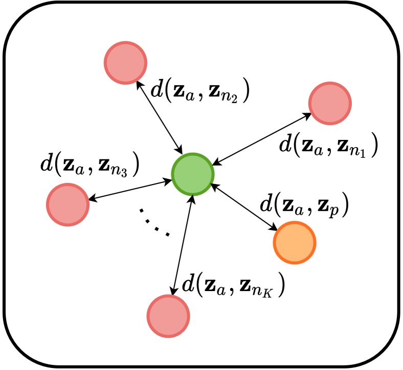
(b) Multiple negative examples.

Fig. 3: A visualisation of the difference in the optimisation of (a) the SiameseRNN and (b) the ContrastiveRNN for a single positive pair $(\mathbf{z}_{a},\mathbf{z}_{p})$ in the embedding space.

3 Acoustic word embeddings for zero-resource languages

In Section 2 we were agnostic to how training targets for the different AWE models are obtained. In this section we describe different strategies for training AWE models, specifically for zero-resource languages where labelled data is not available. One option is to train unsupervised monolingual models directly on unlabelled data (Section 3.1). Another option is to train a supervised multilingual model on labelled data from well-resourced languages and then apply the model to a zero-resource language (Section 3.2). All three of the AWE models in Section 2 can be used in both of these settings, as explained below. Finally, in Section 3.3 we describe a new combined approach where multilingual models are fine-tuned to a zero-resource language using unsupervised adaptation.

3.1 Unsupervised monolingual models

For any of the AWE models in Section 2, we need pairs of segments containing words of the same type; for the SiameseRNN and ContrastiveRNN we additionally need negative examples. In a zero-resource setting there is no transcribed speech to construct such pairs. But pairs can be obtained automatically [53]: we apply an unsupervised term discovery (UTD) system [7] to an unlabelled speech collection from the target zero-resource language. This system discovers pairs of word-like segments, predicted to be of the same unknown type. The discovered pairs can be used to sample positive and negative examples for any of the three models in Section 2. Since the UTD system has no prior knowledge of the language or word boundaries within the unlabelled speech data, the entire process can be considered unsupervised. Using this methodology, we consider purely unsupervised monolingual version of each of the three AWE models in Section 2.

3.2 Supervised multilingual models

Instead of relying on discovered words from the target zero-resource language, we can exploit labelled data from well-resourced languages to train a single multilingual supervised AWE model [31, 32]. This model can then be applied to an unseen zero-resource language. Since a supervised model is trained for one task and applied to another, this can be seen as a form of transfer learning [54, 55]. We consider supervised multilingual variants of the three models in Section 2. Experiments in [31] showed that multilingual versions of the CAE-RNN and SiameseRNN outperform unsupervised monolingual variants. A multilingual ContrastiveRNN hasn’t been considered in a previous study, as far as we know.

3.3 Unsupervised adaptation of multilingual models

While previous studies have found that multilingual AWE models (Section 3.2) are superior to unsupervised AWE models (Section 3.1), one question is whether multilingual models could be tailored to a particular zero-resource language in an unsupervised way. We propose to adapt a multilingual AWE model to a target zero-resource language: a multilingual model’s parameters (or a subset of the parameters) are fine-tuned using discovered word pairs. These discovered segments are obtained by applying a UTD system to unlabelled data from the target zero-resource language. The idea is that adapting the multilingual AWE model to the target language would allow the model to learn aspects unique to that language.

We consider the adaptation of multilingual versions of all three AWE models in Section 2. On development data, we experimented with which parameters to update and which to keep fixed from the source multilingual model. For the CAE-RNN, we found that it is best to freeze the multilingual encoder RNN weights and only update the weights between the final encoder RNN hidden state and the embedding; we also found that it is best to re-initialise the decoder RNN weights randomly before training on the target language. For the SiameseRNN and ContrastiveRNN, we update all weights during adaptation.

As far as we know, we are the first to perform unsupervised adaptation of multilingual AWE models for the zero-resource setting. However, [32] showed the benefit of supervised adaptation, where (limited) labelled data from a target language is used to update the parameters of a multilingual AWE model.

4 Experimental setup

We perform experiments using the GlobalPhone corpus of read speech [56]. As in [57, 31], we treat six languages as our target zero-resource languages: Spanish (ES), Hausa (HA), Croatian (HR), Swedish (SV), Turkish (TR) and Mandarin (ZH). Each language has on average 16 hours of training, 2 hours of development and 2 hours of test data. We apply the UTD system of [7] to the training set of each zero-resource language and use the discovered pairs to train unsupervised monolingual embedding models (Section 3.1). The UTD system discovers around 36k pairs for each language, where pair-wise matching precisions vary between $32\%$ (SV) and $79\%$ (ZH). Training conditions for the unsupervised monolingual CAE-RNN, SiameseRNN and ContrastiveRNN models are determined by doing validation on the Spanish development data. The same hyperparameters are then used for the five remaining zero-resource languages.

For training supervised multilingual embedding models (Section 3.2), six other GlobalPhone languages are chosen as well-resourced languages: Czech, French, Polish, Portuguese, Russian and Thai. Each well-resourced language has on average 21 hours of labelled training data. We pool the data from all six well-resourced languages and train a multilingual CAE-RNN, a SiameseRNN and a ContrastiveRNN. Instead of using the development data from one of the zero-resource languages, we use another well-resourced language, German, for validation of each model before applying it to the zero-resource languages. We only use 300k positive word pairs for each model, as further increasing the number of pairs did not give improvements on the German validation data.

As explained in Section 3.3, we adapt each of the multilingual models to each of the six zero-resource languages using the same discovered pairs as for the unsupervised monolingual models. We again use Spanish development data to determine hyperparameters.

All speech audio is parametrised as $D=13$ dimensional static Mel-frequency cepstral coefficients (MFCCs). All our models have a similar architecture: encoders and decoders consist of three unidirectional RNNs with 400-dimensional hidden vectors, and all models use an embedding size of 130 dimensions. Models are optimised using Adam optimisation [58]. The margin parameter $m$ in Section 2.2 and temperature parameter $\tau$ in Section 2.3 are set to $0.25$ and $0.1$, respectively. We implement all our models in PyTorch.

We use a word discrimination task [59] to measure the intrinsic quality of the resulting AWEs. To evaluate a particular AWE model, a set of isolated test word segments is embedded. For every word pair in this set, the cosine distance between their embeddings is calculated. Two words can then be classified as being of the same or different type based on some distance threshold, and a precision-recall curve is obtained by varying the threshold. The area under this curve is used as final evaluation metric, referred to as the average precision (AP). We are particularly interested in obtaining embeddings that are speaker invariant. We therefore calculate AP by only taking the recall over instances of the same word spoken by different speakers, i.e. we consider the more difficult setting where a model does not get credit for recalling the same word if it is said by the same speaker.

5 Experimental results

We start in Section 5.1 by evaluating the different AWE models using the intrinsic word discrimination task described above. Instead of only looking at word discrimination results, it is useful to also use other methods to try and better understand the organisation of AWE spaces [60], especially in light of recent results [45] showing that AP has limitations. We therefore look at speaker classification performance in Section 5.2, and give a qualitative analysis of adaptation in Section 5.3.

5.1 Word discrimination

We first consider purely unsupervised monolingual models (Section 3.1). We are particularly interested in the performance of the ContrastiveRNN, which has not been considered in previous work. The top section in Table 1 shows the performance for the unsupervised monolingual AWE models applied to the test data from the six zero-resource languages. As a baseline, we also give the results where DTW is used directly on the MFCCs to perform the word discrimination task. We see that the ContrastiveRNN consistently outperforms the CAE-RNN and SiameseRNN approaches on all six zero-resource languages. The ContrastiveRNN is also the only model to perform better than DTW on all six zero-resource languages, which is noteworthy since DTW has access to the full sequences for discriminating between words.

Table 1: AP (%) on test data for the six zero-resource languages. The purely unsupervised monolingual models are trained on discovered word segments (top). The multilingual models are trained on true words by pooling labelled training data from six well-resourced languages (middle). These models are adapted to each of the languages using discovered words from the target zero-resource language (bottom). The best approach in each subsection is shown in bold.

Model	ES	HA	HR	SV	TR	ZH
Unsupervised models:
DTW	$36.2$	$23.8$	$17.0$	$27.8$	$16.2$	$35.9$
CAE-RNN	$52.7$	$18.6$	$24.5$	$28.0$	$14.2$	$33.7$
SiameseRNN	$56.6$	$16.8$	$21.1$	$31.8$	$22.8$	$52.0$
ContrastiveRNN	70.6	36.4	27.8	37.9	31.3	57.1
Multilingual models:
CAE-RNN	$72.4$	$49.3$	$44.5$	52.7	$34.4$	53.9
SiameseRNN	$70.3$	$45.3$	$40.6$	$47.5$	$27.7$	$49.9$
ContrastiveRNN	73.3	50.6	45.1	$46.4$	34.6	$53.2$
Multilingual adapted:
CAE-RNN	$74.2$	$49.4$	45.9	$53.4$	$34.5$	$53.9$
SiameseRNN	$74.5$	$44.7$	$37.6$	$50.3$	$30.3$	$57.3$
ContrastiveRNN	76.6	56.7	$44.4$	54.4	40.5	60.4

Next, we consider the supervised multilingual models (Section 3.2). The middle section of Table 1 shows the performance for the supervised multilingual models applied to the six zero-resource languages. By comparing these supervised multilingual models to the unsupervised monolingual models (top), we see that in almost all cases the multilingual models outperform the purely unsupervised monolingual models, as also in [30, 31]. However, on Mandarin, the unsupervised monolingual ContrastiveRNN model outperforms all three multilingual models. Comparing the three multilingual models, we do not see a consistent winner between the ContrastiveRNN and CAE-RNN, with one performing better on some languages while the other performs better on others. The multilingual SiameseRNN generally performs worst, although it outperforms the ContrastiveRNN on Swedish.

Finally, we consider adapting the supervised multilingual models (Section 3.3). The results after adapting each multilingual model to each of the zero-resource languages are shown in the bottom section of Table 1. Comparing the middle and bottom sections of the table, we see that most of the adapted models outperform their corresponding source multilingual models, with the ContrastiveRNN and SiameseRNN improving substantially after adaptation on some of the languages. The adapted ContrastiveRNN models outperform the adapted CAE-RNN and SiameseRNN models on five out of the six zero-resource languages, achieving some of the best reported results on these data sets [ann+etal_csl20, 30]. We conclude that unsupervised adaptation of multilingual models to a target zero-resource language is an effective AWE approach, especially when coupled with the self-supervised contrastive loss.

Table 2: AP (%) on development data. The supervised monolingual models are trained on ground truth words from the target languages to determine an upper bound on performance. The adapted models are the same as those in Table 1 but applied to development data here for the purpose of analysis.

Model	ES	HA	HR	SV	TR	ZH
Supervised monolingual:
CAE-RNN	$70.2$	$79.7$	$63.0$	$55.8$	$65.6$	$84.2$
SiameseRNN	$78.6$	$85.2$	$79.3$	$68.6$	$77.6$	$93.1$
ContrastiveRNN	$81.8$	$82.4$	$80.3$	$70.9$	$80.5$	$92.1$
Multilingual adapted:
CAE-RNN	$51.7$	$59.5$	$44.3$	$38.6$	$40.9$	$52.2$
SiameseRNN	$51.5$	$52.7$	$38.4$	$40.3$	$33.0$	$56.5$
ContrastiveRNN	$58.0$	$60.5$	$40.5$	$43.8$	$46.9$	$60.2$

One question is whether adapted models close the gap between the zero-resource setting and the best-case scenario where we have labelled data available in a target language. To answer this, Table 2 compares multilingual models (bottom) to “oracle” supervised monolingual models trained on labelled data from the six evaluation languages (top) on development data. Although Table 1 shows that adaptation greatly improves performance in the zero-resource setting, Table 2 shows that multilingual adaptation still does not reach the performance of supervised monolingual models.

5.2 Speaker classification

Table 3: Speaker classification accuracy (%) on development data for the zero-resource languages using purely unsupervised monolingual models (top), multilingual models before adaptation (middle), and models after adaptation (bottom).

Model	ES	HA	HR	SV	TR	ZH
Unsupervised models:
CAE-RNN	$52.8$	$49.5$	$53.8$	$47.8$	$48.9$	$62.0$
SiameseRNN	$38.9$	$38.4$	37.2	$36.4$	$38.6$	$44.3$
ContrastiveRNN	34.6	33.1	$37.8$	33.6	35.5	39.9
Multilingual models:
CAE-RNN	$40.6$	$44.7$	$45.0$	$42.3$	$42.0$	$49.4$
SiameseRNN	$32.6$	$30.3$	$31.9$	28.6	30.3	$32.5$
ContrastiveRNN	27.6	28.7	26.9	$29.2$	$32.1$	31.9
Multilingual adapted:
CAE-RNN	$40.3$	$45.3$	$45.0$	$43.1$	$41.0$	$49.7$
SiameseRNN	$33.6$	$33.9$	$30.6$	29.4	33.7	$37.9$
ContrastiveRNN	30.3	32.1	26.9	$29.5$	$36.5$	35.1

To what extent do the different AWEs capture speaker information? How does adaptation affect speaker invariance? To measure speaker invariance, we use a linear classifier to predict a word’s speaker identity from its AWE. Specifically, we train a multi-class logistic regression model on 80% of the development data and test it on the remaining 20%.

The top section of Table 3 shows speaker classification results on development data for the three types of monolingual unsupervised models (Section 3.1). Since we are interested in how well models abstract away from speaker information, we consider lower accuracy as better (shown in bold). The ContrastiveRNN achieves the lowest speaker classification performance across all languages, except on Croatian where it performs very similarly to the SiameseRNN. This suggests that among the unsupervised monolingual models, the ContrastiveRNN is the best at abstracting away from speaker identity (at the surface level captured by a linear classifier).

Next, we consider speaker classification performance for the multilingual models (Section 3.2). Comparing the middle and top sections of Table 3, we see that for each multilingual model (middle) the speaker classification performance drops from its corresponding unsupervised monolingual version (top) across all six languages, again indicating an improvement in speaker invariance. Comparing the three multilingual models to each other (middle), the ContrastiveRNN has the lowest speaker classification performance on four out of the six evaluation languages.

Finally, we look at the impact of unsupervised adaptation (Section 3.3) on speaker invariance, shown at the bottom of Table 3. After adaptation (bottom) we see that speaker classification results improve consistently compared to their corresponding source multilingual model (middle). Although this seems to indicate that the adapted AWEs capture more speaker information, these embeddings still lead to better word discrimination performance (Table 1). A similar trend was observed in [31]: a model leading to better (linear) speaker classification performance does not necessarily give worse AP. Recent results in [45] showed that AP is limited in its ability to indicate downstream performance for all tasks. Further analysis is required to investigate this seeming contradiction.

Importantly for us, it seems that unsupervised adaptation using unlabelled data in a target zero-resource language leads to representations which better distinguish between speakers in that language.

5.3 Qualitative analysis of adaptation

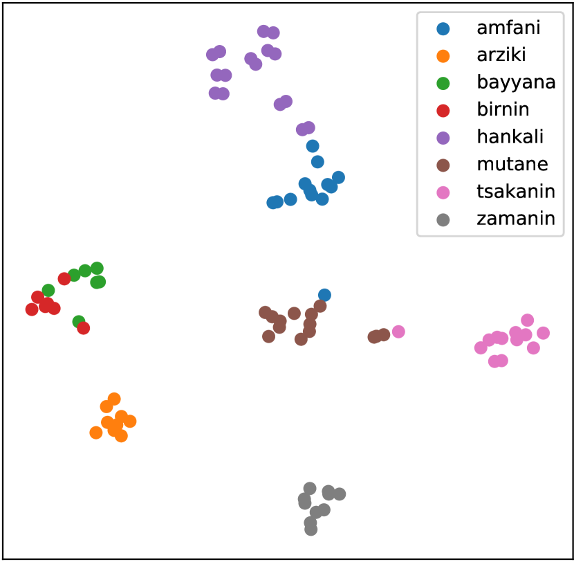
(a) Before adaptation.

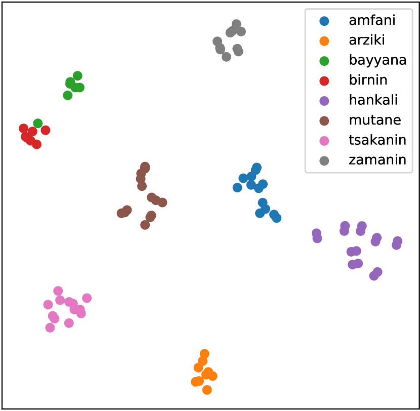
(b) After adaptation.

Fig. 4: t-SNE visualisations of acoustic embeddings for the most frequent words in the Hausa data, produced by (a) the multilingual ContrastiveRNN model and (b) the multilingual ContrastiveRNN model adapted to Hausa.

Figure 4 shows t-SNE visualisations [61] of the AWEs produced by the ContrastiveRNN on Hausa data before and after adaptation. In this curated example, we see how some of the words that are clustered together by the multilingual model (e.g. “amfani” and “hankali”) are separated after adaptation.

6 Conclusion

We have compared a self-supervised contrastive acoustic word embedding approach to two existing methods in a word discrimination task on six zero-resource languages. In a purely unsupervised setting where words from a term discovery system are used for self-supervision, the contrastive model outperformed unsupervised correspondence autoencoder and Siamese embedding models. In a multilingual transfer setting where a model is trained on several well-resourced languages and then applied to a zero-resource language, the contrastive model didn’t show consistent improvements. However, it performed best in a setting where multilingual models are adapted to a particular zero-resource language using the unsupervised discovered word segments, leading to the best reported results on this data. Analysis shows that the contrastive approach abstracts away from speaker identity more than the other two approaches. Future work will involve extending our analysis and performing comparative experiments in a downstream query-by-example search task.

References

- [1] A. Jansen et al., “A summary of the 2012 JHU CLSP workshop on zero resource speech technologies and models of early language acquisition,” in Proc. ICASSP, 2013.
- [2] E. Dunbar, R. Algayres, J. Karadayi, M. Bernard, J. Benjumea, X.-N. Cao, L. Miskic, C. Dugrain, L. Ondel, A. W. Black, et al., “The Zero Resource Speech Challenge 2019: TTS without T,” in Proc. Interspeech, 2019.
- [3] K. Levin, A. Jansen, and B. Van Durme, “Segmental acoustic indexing for zero resource keyword search,” in Proc. ICASSP, 2015.
- [4] S.-F. Huang, Y.-C. Chen, H.-y. Lee, and L.-s. Lee, “Improved audio embeddings by adjacency-based clustering with applications in spoken term detection,” arXiv preprint arXiv:1811.02775, 2018.
- [5] Y. Yuan, C.-C. Leung, L. Xie, H. Chen, B. Ma, and H. Li, “Learning acoustic word embeddings with temporal context for query-by-example speech search,” in Proc. Interspeech, 2018.
- [6] A. S. Park and J. R. Glass, “Unsupervised pattern discovery in speech,” IEEE Trans. Audio, Speech, Language Process., vol. 16, no. 1, pp. 186–197, 2008.
- [7] A. Jansen and B. Van Durme, “Efficient spoken term discovery using randomized algorithms,” in Proc. ASRU, 2011.
- [8] L. Ondel, H. K. Vydana, L. Burget, and J. Černockỳ, “Bayesian subspace hidden markov model for acoustic unit discovery,” arXiv preprint arXiv:1904.03876, 2019.
- [9] O. Räsänen and M. A. C. Blandón, “Unsupervised discovery of recurring speech patterns using probabilistic adaptive metrics,” arXiv preprint arXiv:2008.00731, 2020.
- [10] H. Kamper, K. Livescu, and S. Goldwater, “An embedded segmental k-means model for unsupervised segmentation and clustering of speech,” in Proc. ASRU, 2017.
- [11] S. Seshadri and O. Räsänen, “Sylnet: An adaptable end-to-end syllable count estimator for speech,” IEEE Signal Proc. Let., vol. 26, no. 9, pp. 1359–1363, 2019.
- [12] F. Kreuk, J. Keshet, and Y. Adi, “Self-supervised contrastive learning for unsupervised phoneme segmentation,” in Proc. Interspeech, 2020.
- [13] A. Anastasopoulos, D. Chiang, and L. Duong, “An unsupervised probability model for speech-to-translation alignment of low-resource languages,” in Proc. EMNLP, 2016.
- [14] K. Levin, K. Henry, A. Jansen, and K. Livescu, “Fixed-dimensional acoustic embeddings of variable-length segments in low-resource settings,” in Proc. ASRU, 2013.
- [15] S. Bengio and G. Heigold, “Word embeddings for speech recognition,” in Proc. Interspeech, 2014.
- [16] W. He, W. Wang, and K. Livescu, “Multi-view recurrent neural acoustic word embeddings,” in Proc. ICLR, 2017.
- [17] K. Audhkhasi, A. Rosenberg, A. Sethy, B. Ramabhadran, and B. Kingsbury, “End-to-end ASR-free keyword search from speech,” IEEE J. Sel. Topics Signal Process., vol. 11, no. 8, pp. 1351–1359, 2017.
- [18] Y.-H. Wang, H.-y. Lee, and L.-s. Lee, “Segmental audio word2vec: Representing utterances as sequences of vectors with applications in spoken term detection,” in Proc. ICASSP, 2018.
- [19] Y.-C. Chen, S.-F. Huang, C.-H. Shen, H.-y. Lee, and L.-s. Lee, “Phonetic-and-semantic embedding of spoken words with applications in spoken content retrieval,” in Proc. SLT, 2018.
- [20] N. Holzenberger, M. Du, J. Karadayi, R. Riad, and E. Dupoux, “Learning word embeddings: Unsupervised methods for fixed-size representations of variable-length speech segments,” in Proc. Interspeech, 2018.
- [21] Y.-A. Chung and J. R. Glass, “Speech2vec: A sequence-to-sequence framework for learning word embeddings from speech,” in Proc. Interspeech, 2018.
- [22] A. Haque, M. Guo, P. Verma, and L. Fei-Fei, “Audio-linguistic embeddings for spoken sentences,” in Proc. ICASSP, 2019.
- [23] Y. Shi, Q. Huang, and T. Hain, “Contextual joint factor acoustic embeddings,” arXiv preprint arXiv:1910.07601, 2019.
- [24] S. Palaskar, V. Raunak, and F. Metze, “Learned in speech recognition: Contextual acoustic word embeddings,” in Proc. ICASSP, 2019.
- [25] S. Settle, K. Audhkhasi, K. Livescu, and M. Picheny, “Acoustically grounded word embeddings for improved acoustics-to-word speech recognition,” in Proc. ICASSP, 2019.
- [26] M. Jung, H. Lim, J. Goo, Y. Jung, and H. Kim, “Additional shared decoder on Siamese multi-view encoders for learning acoustic word embeddings,” in Proc. ASRU, 2019.
- [27] Y.-A. Chung, C.-C. Wu, C.-H. Shen, and H.-Y. Lee, “Unsupervised learning of audio segment representations using sequence-to-sequence recurrent neural networks,” in Proc. Interspeech, 2016.
- [28] H. Kamper, “Truly unsupervised acoustic word embeddings using weak top-down constraints in encoder-decoder models,” in Proc. ICASSP, 2019.
- [29] M. Ma, H. Wu, X. Wang, L. Yang, J. Wang, and M. Li, “Acoustic word embedding system for code-switching query-by-example spoken term detection,” arXiv preprint arXiv:2005.11777, 2020.
- [30] H. Kamper, Y. Matusevych, and S. J. Goldwater, “Multilingual acoustic word embedding models for processing zero-resource languages,” in Proc. ICASSP, 2020.
- [31] H. Kamper, Y. Matusevych, and S. Goldwater, “Improved acoustic word embeddings for zero-resource languages using multilingual transfer,” arXiv preprint arXiv:2006.02295, 2020.
- [32] Y. Hu, S. Settle, and K. Livescu, “Multilingual jointly trained acoustic and written word embeddings,” arXiv preprint arXiv:2006.14007, 2020.
- [33] S. Settle and K. Livescu, “Discriminative acoustic word embeddings: Recurrent neural network-based approaches,” in Proc. SLT, 2016.
- [34] C. Doersch and A. Zisserman, “Multi-task self-supervised visual learning,” in Proceedings of the IEEE International Conference on Computer Vision, 2017.
- [35] Y. M. Asano, C. Rupprecht, and A. Vedaldi, “A critical analysis of self-supervision, or what we can learn from a single image,” in Proc. ICLR, 2020.
- [36] C. Doersch, A. Gupta, and A. A. Efros, “Unsupervised visual representation learning by context prediction,” in Proceedings of the IEEE international conference on computer vision, 2015.
- [37] M. Noroozi and P. Favaro, “Unsupervised learning of visual representations by solving jigsaw puzzles,” in Proc. ECCV, 2016.
- [38] S. Gidaris, P. Singh, and N. Komodakis, “Unsupervised representation learning by predicting image rotations,” arXiv preprint arXiv:1803.07728, 2018.
- [39] S. Pascual, M. Ravanelli, J. Serrà, A. Bonafonte, and Y. Bengio, “Learning problem-agnostic speech representations from multiple self-supervised tasks,” arXiv preprint arXiv:1904.03416, 2019.
- [40] G. Synnaeve, Q. Xu, J. Kahn, E. Grave, T. Likhomanenko, V. Pratap, A. Sriram, V. Liptchinsky, and R. Collobert, “End-to-end ASR: from supervised to semi-supervised learning with modern architectures,” arXiv preprint arXiv:1911.08460, 2019.
- [41] A. Baevski, S. Schneider, and M. Auli, “vq-wav2vec: Self-supervised learning of discrete speech representations,” in Proc. ICLR, 2020.
- [42] A. Baevski and A. Mohamed, “Effectiveness of self-supervised pre-training for asr,” in Proc. ICASSP, 2020.
- [43] W. Wang, Q. Tang, and K. Livescu, “Unsupervised pre-training of bidirectional speech encoders via masked reconstruction,” in Proc. ICASSP, 2020.
- [44] M. Ravanelli, J. Zhong, S. Pascual, P. Swietojanski, J. Monteiro, J. Trmal, and Y. Bengio, “Multi-task self-supervised learning for robust speech recognition,” in Proc. ICASSP, 2020.
- [45] R. Algayres, M. S. Zaiem, B. Sagot, and E. Dupoux, “Evaluating the reliability of acoustic speech embeddings,” arXiv preprint arXiv:2007.13542, 2020.
- [46] T. Chen, S. Kornblith, M. Norouzi, and G. E. Hinton, “A simple framework for contrastive learning of visual representations,” arXiv preprint arXiv: 2002.05709, 2020.
- [47] K. Sohn, “Improved deep metric learning with multi-class -pair loss objective,” in Proc. NeurIPS, 2016.
- [48] H. Kamper, W. Wang, and K. Livescu, “Deep convolutional acoustic word embeddings using word-pair side information,” in Proc. ICASSP, 2016.
- [49] S.-I. Ng and T. Lee, “Automatic detection of phonological errors in child speech using siamese recurrent autoencoder,” arXiv preprint arXiv: 2008.03193, 2020.
- [50] K. Q. Weinberger and L. K. Saul, “Distance metric learning for large margin nearest neighbor classification,” J. Mach. Learn. Res., vol. 10, no. Feb, pp. 207–244, 2009.
- [51] G. Chechik, V. Sharma, U. Shalit, and S. Bengio, “Large scale online learning of image similarity through ranking,” J. Mach. Learn. Res., vol. 11, pp. 1109–1135, 2010.
- [52] A. Hermans, L. Beyer, and B. Leibe, “In defense of the triplet loss for person re-identification,” arXiv preprint arXiv:1703.07737, 2017.
- [53] A. Jansen, S. Thomas, and H. Hermansky, “Weak top-down constraints for unsupervised acoustic model training,” in Proc. ICASSP, 2013.
- [54] S. J. Pan and Q. Yang, “A survey on transfer learning,” IEEE Trans. Knowl. Data Eng., vol. 22, no. 10, pp. 1345–1359, 2009.
- [55] S. Ruder, Neural transfer learning for natural language processing, Ph.D. thesis, NUI Galway, Ireland, 2019.
- [56] T. Schultz, N. T. Vu, and T. Schlippe, “GlobalPhone: A multilingual text & speech database in 20 languages,” in Proc. ICASSP, 2013.
- [57] E. Hermann, H. Kamper, and S. J. Goldwater, “Multilingual and unsupervised subword modeling for zero resource languages,” Comput. Speech Language, 2020.
- [58] D. Kingma and J. Ba, “Adam: A method for stochastic optimization,” in Proc. ICLR, 2015.
- [59] M. A. Carlin, S. Thomas, A. Jansen, and H. Hermansky, “Rapid evaluation of speech representations for spoken term discovery,” in Proc. Interspeech, 2011.
- [60] Y. Matusevych, H. Kamper, and S. Goldwater, “Analyzing autoencoder-based acoustic word embeddings,” in BAICS Workshop ICLR, 2020.
- [61] L. van der Maaten and G. Hinton, “Viualizing data using t-SNE,” J. Mach. Learn. Res., vol. 9, pp. 2579–2605, 2008.