Counting mapping class group orbits
under shearing coordinates

Abstract

Let $S_{g,n}$ be an oriented surface of genus $g$ with $n$ punctures, where $2g-2+n>0$ and $n>0$. Any ideal triangulation of $S_{g,n}$ induces a global parametrization of the Teichmüller space $\mathcal{T}_{g,n}$ called the shearing coordinates. We study the asymptotics of the number of the mapping class group orbits with respect to the standard Euclidean norm of the shearing coordinates. The result is based on the works of Mirzakhani.

1 Introduction

There are plenty of results about counting closed geodesics on hyperbolic surfaces. One of the most significant results is Mirzakhani’s count of simple closed geodesics. Let $X$ be a complete hyperbolic metric on $S_{g,n}$ and let $\gamma$ be a simple closed curve. Denote the hyperbolic length of the geodesic representation of $\gamma$ on $X$ by $\ell_{\gamma}(X)$. Let

$$s_{X}(L,\gamma):=\#\{\ \beta\in\mathrm{Mod}_{g,n}\cdot\gamma\ |\ \ell_{\beta}(X)\leqslant L\ \}$$

be the number of simple closed curves in the mapping class group orbit of $\gamma$ with hyperbolic length at most $L$. Mirzakhani [Mir08] proved that, as $L\rightarrow+\infty$,

$$s_{X}(L,\gamma)\sim\frac{n_{\gamma}\cdot B(X)}{b_{g,n}}L^{6g-6+2n}\ .$$

In the above formula, the coefficient $n_{\gamma}$ is determined by the topological type of the curve, and $B(X)$ is an integrable function on the moduli space, endowed with the Weil-Petersson volume form. The integration of $B(X)$ defines the constant $b_{g,n}$. The above result is extended to arbitrary closed curves or multi-curves by Mirzakhani [Mir16], see also [Ara21]. There is also a different proof from other viewpoint, see [ES19].

There are two well-known parametrizations of the Teichmüller space related to the Weil-Petersson symplectic form. One is the Fenchel-Nielsen coordinates, which is defined by choosing a pants decomposition. The other is the shearing coordinates associated to an ideal triangulation (or, in general, a maximal geodesic lamination) [Thu86]. As shown by Mirzakhani [Mir16], by counting the mapping class group orbit of a fixed hyperbolic surface in Teichmüller space, one can understand the distribution of lengths and twists of curves in a random pants decomposition. A similar question is how a random ideal triangulation of a hyperbolic surface looks like.

In this paper, we count the number of the mapping class group orbits in the shearing coordinates. The main result is the following:

Theorem 1.1.

Let $\Delta$ be a given ideal triangulation of $S_{g,n}$, where $2g-2+n>0$ and $n>0$. Let $Sh_{\Delta}:\mathcal{T}_{g,n}\rightarrow\mathbb{R}^{6g-6+3n}$ be the associated shearing coordinates of the Teichmüller space. Then for any $X\in\mathcal{T}_{g,n}$, as $L\rightarrow+\infty$, we have:

$$\#\left\{\ \phi\in\mathrm{Mod}_{g,n}\ \big{|}\ \|Sh_{\Delta}(\phi\cdot X)\|\leqslant L\ \right\}\ \sim\ \frac{n_{\Delta}\cdot B(X)}{b_{g,n}}{L^{6g-6+2n}}\ .$$ (1.1)

Moreover, the coefficient $n_{\Delta}$ is determined by the topological type of $\Delta$ and can be expressed as

$$n_{\Delta}=\mu_{wp}\{\ Y\in\mathcal{T}_{g,n}\ |\ \|Sh_{\Delta}(Y)\|\leqslant 1\ \}.$$

Here $\|\cdot\|$ is the standard Euclidean norm of $\mathbb{R}^{6g-6+3n}$, and $\mu_{wp}$ denotes the Weil-Petersson volume form on the Teichmüller space. Note that for any mapping class $\phi\in\mathrm{Mod}_{g,n}$, $Sh_{\Delta}(\phi\cdot X)=Sh_{\phi^{-1}\cdot\Delta}(X)$. Thus (1.1) counts the number of mapping class group orbit of a given ideal triangulations.

To prove Theorem 1.1, we use the following result of Mirzakhani [Mir16, Theorem 1.1], which is later generalized by Arana-Herrera [Ara20, Theorem 5.5].

Theorem 1.2.

[Mir16, Ara20] Let $\mathcal{F}:\mathcal{T}_{g,n}\rightarrow\mathbb{R}_{+}$ be a positive, continuous, proper function that is asymptotically piecewise linear and bounding with respect to the Fenchel-Nielsen coordinates. Then

$$\lim_{L\to+\infty}\frac{\#\left\{\ \phi\in\mathrm{Mod}_{g,n}\ \big{|}\ \mathcal{F}(\phi\cdot X)\leqslant L\ \right\}}{L^{6g-6+2n}}=\frac{B(X)\cdot r(\mathcal{F})}{b_{g,n}},$$ (1.2)

where

$$r(\mathcal{F}):=\lim_{L\to+\infty}\frac{\mu_{wp}\left\{Y\in\mathcal{T}_{g,n}\ \big{|}\ \mathcal{F}(Y)\leqslant L\right\}}{L^{6g-6+2n}}\ .$$ (1.3)

See §2.2 and §4.1 for the definitions of asymptotically piecewise linear and bounding functions, respectively. The most important examples are hyperbolic lengths of closed curves. To apply Theorem 1.2, we show that the shearing coordinates satisfy the following properties:

(C1) The shear on each edge of $\Delta$ is asymptotically piecewise linear with respect to the Fenchel-Nielsen coordinates. We observe that each shear can be described by an asymptotically piecewise linear function of the hyperbolic lengths of some closed curves. The proof is presented in §3.

(C2). The Euclidean norm of the shearing coordinates is bounding with respect to the Fenchel-Nielsen coordinates. The proof is presented in §4. We first give an equivalent definition of the bounding condition. Then we express the length functions in terms of the shearing coordinates, again in an asymptotically linear way.

To compute the coefficient $r(\mathcal{F})$ in Theorem 1.2 when $\mathcal{F}$ is the shearing norm, we show that the Weil-Petersson volume form is equal to Euclidean volume form under the shearing coordinates, up to a scaling constant. This is done in §5.

Acknowledgements. We would like to thank for useful discussions, and for numerous useful comments and corrections.

2 Preliminaries

2.1 Teichmüller space and Fenchel-Nielsen coordinates

We recall some basic notions from the theory of Teichmüller spaces. For more details, see [FM, Hu].

Given a topological surface $S_{g,n}$, its Teichmüller space $\mathcal{T}_{g,n}$ is the space of all complete hyperbolic metrics up to isotopy. More precisely, a point in $\mathcal{T}_{g,n}$ is an equivalence class of pairs $(f,\Sigma)$, where $f$ is an orientation-preserving homeomorphism from $S_{g,n}$ to a complete hyperbolic surface $\Sigma$. Two pairs $(f_{1},\Sigma_{1})$ and $(f_{2},\Sigma_{2})$ are equivalent if and only if $f_{2}\circ f_{1}^{-1}$ is homotopic to an isometry from $\Sigma_{1}$ to $\Sigma_{2}$.

Let $\gamma$ be a closed curve on $S_{g,n}$, which is neither homotopic to a point nor to a puncture. Given $X\in\mathcal{T}_{g,n}$ represented by a pair $(f,\Sigma)$, the curve $f(\gamma)$ is freely homotopic to a unique closed geodesic on $\Sigma$. The hyperbolic length of $f(\gamma)$ on $\Sigma$ depends on the equivalence class of the pair. Thus it defines a function on $\mathcal{T}_{g,n}$ called the length function of $\gamma$, denoted by $\ell_{\gamma}$.

The hyperbolic length can also be expressed by the trace of matrix. If $X\in\mathcal{T}_{g,n}$ is corresponding to a Fuchsian representation $\rho_{X}:\pi_{1}(S_{g,n})\to\mathrm{PSL}(2,\mathbb{R})$, then for any closed curve $\gamma\in\pi_{1}(S_{g,n})$, we have

$$\big{|}\mathrm{tr}\big{(}\rho_{X}(\gamma)\big{)}\big{|}=\cosh\left(\frac{\ell_{\gamma}(X)}{2}\right)\ .$$ (2.1)

Let $\mathrm{Mod}_{g,n}$ be the mapping class group of $S_{g,n}$, i.e. the group of isotopy classes of orientation-preserving self-homeomorphisms leaving each puncture fixed. Then $\mathrm{Mod}_{g,n}$ acts on $\mathcal{T}_{g,n}$ by changing the markings. If $X\in\mathcal{T}_{g,n}$ is represented by $(f,\Sigma)$ and $\phi\in\mathrm{Mod}_{g,n}$, then $\phi\cdot X\in\mathcal{T}_{g,n}$ is represented by $(f\circ\phi^{-1},\Sigma)$. In particular, for a closed curve $\gamma$, we have $\ell_{\gamma}(\phi\cdot X)=\ell_{\phi^{-1}\cdot\gamma}(X)$. The action of $\mathrm{Mod}_{g,n}$ on $\mathcal{T}_{g,n}$ is properly discontinuous, thus the orbit of any point is discrete.

Recall that a pair of pants is a topological surface homeomorphic to $S_{0,3}$. A pants decomposition of $S_{g,n}$ is a set of disjoint simple closed curves which decompose the surface into pairs of pants. Let $\mathcal{P}=\{\alpha_{i}\}_{i=1}^{3g-3+n}$ be a pants decomposition of $S_{g,n}$. The Fenchel-Nielsen coordinates adapted to $\mathcal{P}$ consist of the length functions of $\alpha_{i}$ and the twist parameters $\tau_{\alpha_{i}}$ along $\alpha_{i}$. For the precise definition of twist parameter, see [Bu, $\mathbf{\S}$3.3]. We have a homeomorphism

$$\mathrm{FN}_{\mathcal{P}}:\mathcal{T}_{g,n} \longrightarrow\mathbb{R}_{+}^{3g-3+n}\times\mathbb{R}^{3g-3+n}$$

$$X \longmapsto\big{(}l_{\alpha_{i}}(X),\tau_{\alpha_{i}}(X)\big{)}\ .$$

The Fenchel-Nielsen coordinates induce a canonical symplectic 2-form on $\mathcal{T}_{g,n}$, which is called the Weil-Petersson symplectic form. A remarkable fact due to Wolpert [Wol82] is that the Weil-Petersson symplectic form does not depend on the choice of the pants decomposition. Thus it gives a volume form $\mu_{wp}$ on $\mathcal{T}_{g,n}$ which is invariant under the action of the mapping class group.

2.2 Asymptotically piecewise linear functions

We introduce the notion of asymptotically piecewise linear function, following [Mir16, §4].

A closed cone $\mathcal{C}\subset\mathbb{R}^{k}$ is a noncompact closed region bounded by finitely many hyperplanes, that is,

$$\mathcal{C}=\bigcap_{i=1}^{m}\big{\{}\ \vec{x}\in\mathbb{R}^{k}\ \big{|}\ \mathcal{R}_{i}(\vec{x})\geqslant 0\ \big{\}},$$

where each $\mathcal{R}_{i}(\vec{x})=r_{i}^{1}x_{1}+\cdots+r_{i}^{k}x_{k}$ is a linear function.

We say that $\vec{x}$ tends to infinity in $\mathcal{C}$, denoted by $\vec{x}\to\mathcal{C}_{\infty}$, if $\vec{x}$ stays within the closed cone $\mathcal{C}$ and

$$\min_{i=1\cdots m}\big{\{}\ \mathcal{R}_{i}(\vec{x})\ \big{\}}\rightarrow+\infty\ .$$

Geometrically, this means that $\vec{x}$ stays asymptotically away from the boundary of $\mathcal{C}$.

Let $F:\mathcal{C}\to\mathbb{R}$ be a function on a closed cone. We say that $F$ is asymptotically linear if there exists a linear function $\mathcal{L}:\mathcal{C}\to\mathbb{R}$ and some real number $c$ such that

$$\lim_{\vec{x}\to\mathcal{C}_{\infty}}\big{(}F(\vec{x})-\mathcal{L}(\vec{x})\big{)}=c\ .$$

For this we write $F\sim\mathcal{L}$ in $\mathcal{C}$. Note that $F\sim\mathcal{L}$ in $\mathcal{C}$ if and only if for any $\varepsilon>0$, there exists $A>0$ such that

$$\big{|}F(\vec{x})-\big{(}\mathcal{L}(\vec{x})+c\big{)}\big{|}<\varepsilon$$

for any $\vec{x}\in\mathcal{C}$ satisfying $\min\{\mathcal{R}_{i}(\vec{x})\}>A$.

Roughly speaking, being asymptotically linear means that, far away from the hyperplanes, the function behaves asymptotically like a linear function. Simple examples of asymptotically linear functions are $\cosh^{-1}(e^{x})$ and $\sinh^{-1}(e^{x})$. We have

$$\cosh^{-1}(e^{x})\sim x,\ \sinh^{-1}(e^{x})\sim x\ \mathrm{in}\ \mathbb{R}_{+}\ .$$

A function is defined to be asymptotically piecewise linear, if one can divide its domain of definition into finitely many closed cones such that the function is asymptotically linear on each cone. Similarly, a vector-valued function $\mathbf{F}$ is asymptotically (piecewise) linear if each component is asymptotically (piecewise) linear. Equivalently, there exists a linear transformation $\mathcal{L}:\mathbb{R}^{k}\to\mathbb{R}^{l}$ and $\vec{c}\in\mathbb{R}^{l}$ such that

$$\|\mathbf{F}(\vec{x})-\big{(}\mathcal{L}(\vec{x})+\vec{c}\ \big{)}\|\to 0$$

as $\vec{x}\to\mathcal{C}_{\infty}$. We will use the abbreviation “A(P)L” for ”asymptotically (piecewise) linear” throughout this paper.

The following composition law is easy to prove.

Proposition 2.1 (Composition law for APL functions).

Let $\mathcal{C}$ be a closed cone in $\mathbb{R}^{k}$ and let $F_{i}:\mathcal{C}\to\mathbb{R}$ be APL functions for $i=1,\cdots,m$. Let $\mathcal{C}^{\prime}$ be a closed cone in $\mathbb{R}^{m}$ and let $G:\mathcal{C^{\prime}}\to\mathbb{R}$ be an APL function. Assume that for all $\vec{x}\in\mathcal{C}$, $\big{(}F_{1}(\vec{x}),\cdots,F_{m}(\vec{x})\big{)}\in\mathcal{C^{\prime}}$. Then $H:=G\big{(}F_{1},\cdots,F_{m}\big{)}$ is again an ALP function.

Given a family $\mathcal{M}$ of APL funcitons, let $\mathfrak{F}$ be the set of functions generated by $\mathcal{M}$, under arithmetic operations, rational multiplication or $N$-th root:

$$f\pm g\ ,\ f\cdot g\ ,\ \frac{f}{g}\ ,\ r\cdot f\ ,\ \sqrt[N]{f}\ .$$

Then for each $f\in\mathfrak{F}$, the functions $\sinh^{-1}(e^{f}),\cosh^{-1}(e^{f})$ are APL. In this paper, all APL functions we considered are obtained from such construction.

The following basic result is due to Mirzakhani [Mir16, Theorem 4.1]:

Proposition 2.2.

For any closed curve $\gamma$ on $S_{g,n}$, the hyperbolic length function $\ell_{\gamma}:\mathcal{T}_{g,n}\to\mathbb{R}_{+}$ is an APL function with respect to any given Fenchel-Nielsen coordinates.

In fact, Mirzakhani [Mir16] shows that the transformation between Fenchel-Nielsen coordinates associated to any two different pants decomposition is APL. Thus the property of being APL with respect to Fenchel-Nielsen coordinates does not depend on the the choice of the pants decomposition.

3 The Shearing Coordinates

The shearing coordinates of $\mathcal{T}_{g,n}$ was introduced by Thurston[Thu86]. We will show that, for any ideal triangulation, the shear on each edge is an APL function with respect to the Fenchel-Nielsen coordinates.

3.1 Shear between adjacent triangles

Let $T_{1},T_{2}$ be a pair of adjacent ideal geodesic triangles in the hyperbolic plane, with a common edge $c$. Note that all ideal geodesic triangles are isometric. An ideal triangle has a unique inscribed circle tangent to its three edges. Denote the tangent points of the inscribed circles on the common edge $c$ by $p_{i}\ (i=1,2)$.

Definition 3.1.

The shear on the common edge $c$ of two adjacent ideal triangles $T_{1},T_{2}$ is the signed distance from $p_{1}$ to $p_{2}$, denoted by $s_{c}$. Here $c$ is oriented such that $T_{1}$ is on the left and $T_{2}$ is on the right.

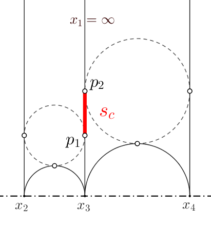
Figure 1: Shear between two adjacent ideal triangles. Here $s_{c}>0$ .

One can check that interchanging the order of $T_{1},T_{2}$ does not change the shear. See Figure 1 for the case of a positive shear.

The following formula relates shear with cross-ratio. We adopt the upper half plane model for the hyperbolic plane. The ideal boundary $\partial\mathbb{H}$ is identified with $\mathbb{R}\cup\{\infty\}$. Denote the geodesic with two different end points $x,y\in\partial\mathbb{H}$ by $[x,y]$. And denote the ideal triangle with three different ideal vertices $x,y,z\in\partial\mathbb{H}$ by $[x,y,z]$.

Proposition 3.2.

Let $x_{1},x_{2},x_{3},x_{4}$ be four distinct points on $\partial\mathbb{H}$, in counterclockwise order. Let $T_{1}=[x_{1},x_{2},x_{3}]$ and $T_{2}=[x_{1},x_{3},x_{4}]$, with the common edge $c=[x_{1},x_{3}]$. Then

$$s_{c}=\ln\frac{(x_{1}-x_{2})(x_{3}-x_{4})}{(x_{1}-x_{4})(x_{2}-x_{3})}\ .$$ (3.1)

3.2 The shearing coordinates

Let $\Delta$ be an ideal triangulation on $S_{g,n}$. For any $X\in\mathcal{T}_{g,n}$ represented by $(f,\Sigma)$, $f(\Delta)$ is homotopic to an ideal geodesic triangulation of $\Sigma$. For each edge $c\in\Delta$, the shearing on $f(c)$ under the hyperbolic metric of $\Sigma$ is denoted by $s_{c}(X)$. (To define $s_{c}(X)$, we can lift the map $f:S_{g,n}\to\Sigma$ to the universal covers.) Note that $s_{c}(X)$ is independent of the choice of the representation $(f,\Sigma)$, thus well-defined on $\mathcal{T}_{g,n}$.

We can recover the hyperbolic structure by gluing those hyperbolic ideal triangles with the data of triangulation and shears. See Figure 2 for an example, which shows an ideal triangulation of $S_{1,1}$ in the universal covering space.

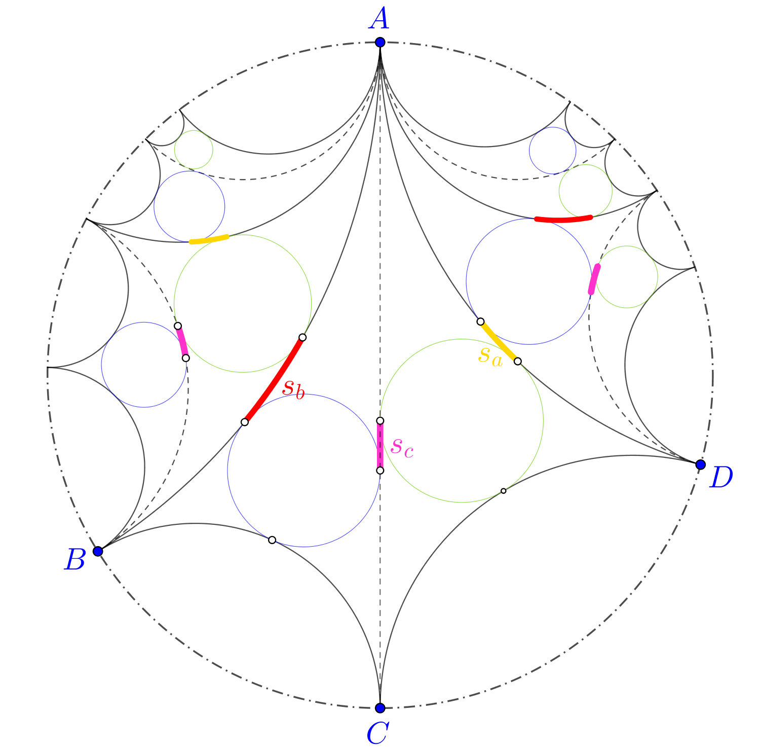
Figure 2: An ideal triangulation of $S_{1,1}$ in $\mathbb{D}$. The ideal quadrilateral $ABCD$ is a fundamental domain. The shear on each edge is labelled as a colored segment.

Theorem 3.3.

[BBFS13, Theorem 3.6] The map $Sh_{\Delta}$ $:\mathcal{T}_{g,n}\to\mathbb{R}^{6g-6+3n}$, defined by

$$Sh_{\Delta}(X):=(s_{c}(X))_{c\in\Delta}\ ,$$

is a homeomorphism onto its image.

The shear parameters are not all independent. At each puncture, the completeness of the hyperbolic structure induces a linear equation of the shears on the edges emitting from it. In fact the sum of these shears should be zero. Since there are $n$ punctures, there are $(6g-6+2n)$ independent parameters, which coincides with the dimension of $\mathcal{T}_{g,n}$.

Proposition 3.4.

The shearing coordinates reduces to a homeomorphism from $\mathcal{T}_{g,n}$ to a linear subspace $\mathcal{C}_{\Delta}$ of dimension $(6g-6+2n)$.

See [BBFS13] for the proofs.

3.3 Relation between shear and length

Let $X=(f,\Sigma)$ be a point in $\mathcal{T}_{g,n}$, and let $\Gamma$ be a Fuchsian group such that $\Sigma=\mathbb{H}/\Gamma$. In the following, we use the trace formula (2.1) to represent the shear as a function of hyperbolic lengths. $\Gamma$.

Since each ideal vertex is corresponding to a fixed point of some parabolic element in $\Gamma$, we first recall some basic properties of parabolic elements in $\mathrm{SL}_{2}(\mathbb{R})$.

Lemma 3.5.

Suppose that $g=\left[\begin{smallmatrix}A&B\\ C&D\\ \end{smallmatrix}\right]\in\mathrm{SL}_{2}(\mathbb{R})$ is a parabolic element. Then
1. $\left|\mathrm{tr}\left(g\right)\right|=\left|A+D\right|=2$;
2. The unique fixed point of $g$ on the ideal boundary is $x=\frac{A-D}{2C}$.

Proposition 3.6.

Suppose that

$${g}_{i}=\left[\begin{matrix}{{A}_{i}}&{{B}_{i}}\\ {{C}_{i}}&{{D}_{i}}\\ \end{matrix}\right]\in\mathrm{SL}_{2}(\mathbb{R}),\ i=1,2$$

represent two parabolic elements in the Fuchsian group $\Gamma$, with fixed point $x_{1},x_{2}\neq\infty$ on the boundary. Then

$${\rm tr}\left({{g}_{1}}\cdot{{g}_{2}}\right)=\frac{1}{2}{\rm tr}\left({{g}_{1}}\right){\rm tr}\left({{g}_{2}}\right)-{{C}_{1}}{{C}_{2}}{{\left({{x}_{1}}-{{x}_{2}}\right)}^{2}}.$$ (3.2)

In particular, ${{C}_{1}}{{C}_{2}}{{\left({{x}_{1}}-{{x}_{2}}\right)}^{2}}$ is invariant under conjugation.

Proof.

By Lemma 3.5, one gets the equations for $i=1,2$:

$$A_{i}D_{i}-B_{i}C_{i}=1,$$

$${{\left(A_{i}+D_{i}\right)}^{2}}=4,$$

$$A_{i}-D_{i}=2x_{i}C_{i}.$$

Note that $x_{i}\neq\infty$ implies $C_{i}\neq 0$. Solve for $B_{i},D_{i}$ :

$$D_{i}=A_{i}-2x_{i}C_{i},$$

$$B_{i}=-{{x_{i}}^{2}}C_{i}.$$

Then

$$\textrm{tr}\left({{g}_{1}}\cdot{{g}_{2}}\right) =A_{1}A_{2}+B_{1}C_{2}+B_{2}C_{1}+D_{1}D_{2}$$

$$=2(A_{1}-x_{1}C_{1})(A_{2}-x_{2}C_{2})-C_{1}C_{2}(x_{1}-x_{2})^{2}$$

$$=2\left(A_{1}-\frac{A_{1}-D_{1}}{2}\right)\left(A_{2}-\frac{A_{2}-D_{2}}{2}\right)-C_{1}C_{2}(x_{1}-x_{2})^{2}\ .$$

∎

Remark 3.7.

If $g_{1}$ and $g_{2}$ are distinct parabolic elements, then either $g_{1}g_{2}$ or $g_{1}g_{2}^{-1}$ is hyperbolic.

Corollary 3.8.

Let $T_{1},T_{2}$ be a pair of adjacent ideal triangles on $S_{g,n}$, with common edge $c$. There exist four closed curves $\gamma_{1},\gamma_{2},\gamma_{3},\gamma_{4}$ on $S_{g,n}$ such that $s_{c}(X)$ is an APL function of the hyperbolic length of $\gamma_{i}$:

$$s_{c}(X)=F_{c}\bigg{(}\ell_{\gamma_{1}}(X),\ell_{\gamma_{2}}(X),\ell_{\gamma_{3}}(X),\ell_{\gamma_{4}}(X)\bigg{)}\ .$$

The closed curves and the APL function depend only on the topology of $T_{1},T_{2}$.

Proof.

Denote $\Sigma$ by $\mathbb{H}/\Gamma$ as before. Let $\widetilde{T_{1}},\widetilde{T_{2}}$ be a pair of adjacent preimage of $T_{1},T_{2}$, with ideal vertices $x_{1},x_{2},x_{3},x_{4}$ in counterclockwise order and a common edge $[x_{1},x_{3}]$.

Each $x_{i}$ corresponds to a primitive parabolic element $g_{i}\in\Gamma$. We may also assume that all $C_{i}\neq 0$, otherwise we can replace $\Gamma$ by an appropriate conjugation. For $i\neq j$, let $\gamma_{ij}$ be the closed curve corresponding to the invariant geodesic axis of the hyperbolic element $g_{i}g_{j}$ or $g_{i}g_{j}^{-1}$. Combining formula (2.1) with Proposition 3.6, we have:

$$-{{C}_{i}}{{C}_{j}}\left({x}_{i}-{x}_{j}\right)^{2}=\pm 2\cosh\left(\frac{\ell_{\gamma_{ij}}(X)}{2}\right)-\frac{{\rm tr}(g_{i}){\rm tr}(g_{j})}{2},$$

where ${\rm tr}(g_{i})=\pm 2$ are constants.

Since $x_{i}\neq 0$, we can rewrite formula (3.1) as

$$s_{c}(X) =\frac{1}{2}\ln\frac{C_{1}C_{2}(x_{1}-x_{2})^{2}C_{3}C_{4}(x_{3}-x_{4})^{2}}{C_{1}C_{4}(x_{1}-x_{4})^{2}C_{2}C_{3}(x_{2}-x_{3})^{2}}\ .$$

It is easy to verify that $s_{c}(X)$ is APL with respect to the four length functions (using the discussion after Proposition 2.1).

Given a pair of ideal triangles, the choices of $g_{i}$’s and $\gamma_{ij}$’s only depend on the fundamental group of the surface. Since $\mathcal{T}_{g,n}$ is simply connected, when the hyperbolic structure on the surface changes continuously in $\mathcal{T}_{g,n}$, all signs appeared in the above function remains the same. As a result, the function is determined by topology. ∎

Given an ideal triangulation $\Delta$, for each edge $c\in\Delta$ we can choose four closed curves and a function $F_{c}$ as above. By Proposition 2.2, each variable in Corollary 3.8 is an APL function with respect to the Fenchel-Nielsen coordinates. By the composition law in Proposition 2.1, we obtain:

Theorem 3.9.

Given an ideal triangulation $\Delta$ on the surface $S_{g,n}$, the shearing coordinates  $Sh_{\Delta}:\mathcal{T}_{g,n}\to\mathbb{R}^{6g-6+3n}$ is APL with respect to the Fenchel-Nielsen coordinates.

4 Mirzakhani’s counting result and the bounding condition

The original bounding condition in Theorem 1.2 is proposed by Mirzakhani [Mir16]. It is used to reduce the counting problem in the Teichmüller space to a problem in some specific cone-shaped region. Here we adopt the definition in [Ara20].

4.1 Restatement of the bounding condition

Under the Fenchel-Nielsen coordinates $(\ell_{i},\tau_{i})_{i=1}^{3g-3+n}$ adapted to some pants decomposition $\mathcal{P}$, the Teichmüller space $\mathcal{T}_{g,n}$ admits a partition into countably many convex polytopes of the form

$$\mathcal{C}_{\mathcal{P}}^{\mathbf{m}}:=\bigg{\{}\ Y\in\mathcal{T}_{g,n}\ \bigg{|}\ m_{i}\cdot\ell_{i}(Y)\leqslant\tau_{i}(Y)\leqslant(m_{i}+1)\cdot\ell_{i}(Y)\ \bigg{\}}$$

with $\mathbf{m}:=(m_{1},\cdots,m_{3g-3+n})\in\mathbb{Z}^{3g-3+n}$.

Definition 4.1.

A funciton $\mathcal{F}:\mathcal{T}_{g,n}\rightarrow\mathbb{R}_{+}$ is bounding with respect to the Fenchel-Nielsen coordinates $(\ell_{i},\tau_{i})_{i=1}^{3g-3+n}$, if for every $Y\in\mathcal{T}_{g,n}$ there exists a constant $C>0$ such that for every $\mathbf{m}\in\mathbb{Z}^{3g-3+n}$ and every $Z\in\mathrm{Mod}_{g,n}\cdot Y\cap\mathcal{C}_{\mathcal{P}}^{\mathbf{m}}\cap\mathcal{F}^{-1}([0,L])$,

$$\ell_{i}(Z)\leqslant C\cdot\frac{L}{\max\{|m_{i}|,|m_{i}+1|\}}\ .$$ (4.1)

This means that, when the value of $\mathcal{F}$ grows, the length of the $i$-th pants curve grows at a linear rate, and it is also proportional to the twist component.

Proposition 4.2.

The bounding condition (4.1) is equivalent to the following condition:
for every $Y\in\mathcal{T}_{g,n}$,

$$\sup_{Z\in\mathrm{Mod}_{g,n}\cdot Y}\left\{\frac{\ell_{i}(Z)+|\tau_{i}(Z)|}{\mathcal{F}(Z)}\right\}<+\infty\ .$$ (4.2)

Proof.

We write $\ell_{i}=\ell_{i}(Z)$ and $\tau_{i}=\tau_{i}(Z)$ for simplicity.

Suppose (4.1) holds. When $m_{i}\geqslant 0$ and $Z\in\mathcal{C}_{\mathcal{P}}^{\mathbf{m}}$, we have $0\leqslant m_{i}\leqslant\tau_{i}/\ell_{i}\leqslant m_{i}+1$. Then

$$C\geqslant(m_{i}+1)\frac{\ell_{i}}{\mathcal{F}} \geqslant\frac{m_{i}+2}{2}\frac{\ell_{i}}{\mathcal{F}}$$

$$=\frac{\ell_{i}+(m_{i}+1)\ell_{i}}{2\mathcal{F}}\geqslant\frac{\ell_{i}+\tau_{i}}{2\mathcal{F}}\ .$$

Thus

$$\frac{\ell_{i}+\tau_{i}}{\mathcal{F}}\leqslant 2C\ .$$

When $m_{i}<0$, we have $0\leqslant-m_{i}-1\leqslant|\tau_{i}|/\ell_{i}\leqslant-m_{i}$. Then

$$C\geqslant(-m_{i})\frac{\ell_{i}}{\mathcal{F}} \geqslant\frac{-m_{i}+1}{2}\frac{\ell_{i}}{\mathcal{F}}$$

$$=\frac{\ell_{i}+(-m_{i})\ell_{i}}{2\mathcal{F}}\geqslant\frac{\ell_{i}+|\tau_{i}|}{2\mathcal{F}}\ .$$

So (4.2) holds.

Now suppose $\mathcal{F}$ satisfies (4.2), with upper bound $K>0$. If $Z\in\mathrm{Mod}_{g,n}\cdot Y$ with
$0\leqslant m_{i}\leqslant\tau_{i}/\ell_{i}\leqslant m_{i}+1$, then

$$K\geqslant\frac{\ell_{i}+\tau_{i}}{\mathcal{F}}\geqslant\frac{\ell_{i}+m_{i}\ell_{i}}{\mathcal{F}}\ .$$

If $m_{i}\leqslant\tau_{i}/\ell_{i}\leqslant m_{i}+1\leqslant 0$, then

$$K\geqslant\frac{\ell_{i}-\tau_{i}}{\mathcal{F}}\geqslant\frac{\ell_{i}-(m_{i}+1)\ell_{i}}{\mathcal{F}}=\frac{-m_{i}\ell_{i}}{\mathcal{F}}\ .$$

Thus (4.1) holds.

Note that each part of the proof utilizes one side of the condition $m_{i}\leqslant\tau_{i}/\ell_{i}\leqslant m_{i}+1$.

∎

4.2 Relation between length and shear

Our aim here is to prove that ${\mathcal{F}(X)}=\|Sh_{\Delta}(X)\|$ satisfies the inequality (4.2). In the following theorem, we have a formula of the length function in terms of shears. This is the key result in this paper.

Theorem 4.3.

Let $\gamma$ be a non-degenerated closed curve on $S_{g,n}$, and let $X\in\mathcal{T}_{g,n}$ represented by $\mathbb{H}/\Gamma$. Let $g\in\Gamma$ be a primitive hyperbolic element corresponding to $\gamma$. Let $(s_{1},\cdots,s_{K})=Sh_{\Delta}(X)$ be the shearing coordinates of $X$ associated to the triangulation $\Delta$. Then $|\mathrm{tr}(g)|=2\cosh(\ell_{\gamma}(X)/2)$ is a polynomial of variables $\{e^{\pm s_{j}/2}\}_{j=1}^{K}$ with rational coefficients:

$$\cosh(\ell_{\gamma}/2)\in\mathbb{Q}\big{[}e^{\pm s_{1}/2},\cdots,e^{\pm s_{K}/2}\big{]}\ .$$

The polynomial only depends on the topological type of $\Delta$ and $\gamma$.

Proof.

We will give a precise algorithm to compute the matrix $g\in\mathrm{SL}_{2}(\mathbb{R})$.

Passing to the universal cover, we fix an orientation of $\gamma$ and choose one intersection of $\gamma$ and $\Delta$ as an initial point (here we have identify $\gamma$ with the axis of $g$). Up to a conjugation, we may assume that the initial point of $\gamma$ is the complex number $i$ in the upper half plane, contained in the ideal triangle $T_{1}=[-1,1,\infty]$.

Traveling forward along $\gamma$, we have a sequence of triangles $(T_{1},\cdots,T_{N+1}=gT_{1})$. Let $a_{i}$ be the common ideal edge of $T_{i},T_{i+1}$, $i=1,\cdots,N$. The sequence $\left(a_{i}\right)_{i=1}^{N}$ depends only on the type of $\gamma$ and $\Delta$, thus a topological data. The shear on $a_{i}$ is denoted by $s_{i}$. Our algorithm consists of three steps:

(1) The initial data: “Left $\&$ Right sequences”.

If $\gamma$ enters $T_{i}$ through one edge, then it must leave through one of the other two edges. Given the orientation of $X$ and $\gamma$, one can tell $\gamma$ leave the triangle through the left edge or the right edge. Thus we can say that $T_{i+1}$ lies on the left or on the right hand side of $T_{i}$. Define $\varepsilon_{i}=+1$ if $T_{i+1}$ lies on the left, $\varepsilon_{i}=-1$ if on the right. See Figure 3 for illustration and examples.

(a) Turn left, or $\varepsilon=+$.

(b) Turn right, or $\varepsilon=-$.

(c) From $T_{1}$ to $T_{4}$, the sequence is $(-,+,-).$

Figure 3: The ’left-right sequences’.

Then we get a sequence of signatures $\left(\varepsilon_{i}\right)_{i=1}^{N}$, which tells how $\gamma$ passing through each triangles along the path.

(2) The basic matrices of shear.

The initial data characterizes how $\gamma$ passing through each triangle. Now we construct the basic matrices of Möbius transformation corresponding to the shear deformation.

If $\gamma$ leaves through the right edge, we may first apply a Möbius transformation $R$ to map $(-1,i,1)$ into $(\infty,1+2i,1)$. Then the two triangles $T_{1},R(T_{1})$ have a common edge $[1,\infty]$ with coincide tangent points. If $\gamma$ leaves through the left edge, we map $(-1,i,1)$ into $(-1,-1+2i,\infty)$. The corresponding matrices are

$$R:=\frac{1}{2}\left(\begin{array}[]{cc}3&-1\\ 1&1\\ \end{array}\right),\ L:=\frac{1}{2}\left(\begin{array}[]{cc}3&1\\ -1&1\\ \end{array}\right)$$

To unify them, we may define

$$P_{\varepsilon}:=\frac{1}{2}\left(\begin{array}[]{cc}3&\varepsilon\\ -\varepsilon&1\\ \end{array}\right),\ \varepsilon=\pm 1$$

Then $R=P_{-},\ L=P_{+}$.

We have mapped the entering edge onto the leaving edge by $P_{\varepsilon}$ as above. If $\gamma$ leave through the right edge, then shearing along the leaving edge means applying a hyperbolic transformation with fixed point $\{1,\infty\}$ and signed translation distance $s$. In complex coordinate, the function is $z\mapsto e^{s}(z-1)+1$. Similarly, for the left edge case, the complex function is $z\mapsto e^{-s}(z+1)-1$. The unified matrices are

$$H_{\varepsilon}(s):=\left(\begin{array}[]{cc}e^{\ -{\varepsilon s}/{2}}&-\sinh(s/2)\\ 0&e^{\ {\varepsilon s}/{2}}\\ \end{array}\right)$$

Some calculation shows that the third vertex of $(H_{\varepsilon}(s)\circ P_{\varepsilon})(T_{1})$ other than $\pm 1,\infty$ is
$-\varepsilon(1+2e^{-\varepsilon s})$.

In conclusion, we take ${V_{\varepsilon}(s)}:=H_{\varepsilon}(s)\circ P_{\varepsilon}$. It maps $T_{1}$ to the next triangle along $\gamma$.

(3) The composition diagram.

Let $g$ be a primitive hyperbolic element, corresponding to the translation along $\gamma$ for a single period. We now compute the matrix representation for $g$. It is a composition of basic matrices defined as above.

Let $\left(T_{i}\right)_{i=1}^{N},\left(a_{i}\right)_{i=1}^{N},\left(\varepsilon_{i}\right)_{i=1}^{N}$ as before. Denote by $a_{0}$ be the edge at which $\gamma$ enters $T_{1}$. For any $i=1,\cdots,N$, there is a unique isometry $f_{i}$ that maps $T_{i}$ into $T_{i+1}$ with the edge $a_{i-1}$ matching $a_{i}$. Then

$$g=f_{N}\circ\cdots\circ f_{1}.$$

Denote $V_{\varepsilon_{i}}(s_{\varepsilon_{i}})$ by $V_{i},i=1,\cdots,N$ to simplify notations. Note that $f_{1}=V_{1}$.

We have the following diagram:

By going to the bottom right corner diagonally and then going up, one get

$$g =V_{1}\circ V_{2}\circ\cdots V_{N-1}\circ V_{N}\circ V_{N-1}^{-1}\cdots\circ V_{2}^{-1}\circ V_{2}\circ V_{1}^{-1}\circ f_{1}$$

$$=V_{1}\circ V_{2}\circ\cdots V_{N-1}\circ V_{N}$$

$$=H_{\varepsilon_{1}}(s_{1})P_{\varepsilon_{1}}\cdots H_{\varepsilon_{N}}(s_{N})P_{\varepsilon_{N}}\ .$$

It is obvious that each element in the matrix is a polynomial of $e^{\ \pm s_{i}/2}$, with rational coefficients. The polynomials are determined by topology. ∎

For the twist $\tau_{i}$ on each pants curve, we have a similar result.

Corollary 4.4.

With the notations in Definition 4.1 and Theorem 4.3, we have:

$$\cosh^{2}(\tau_{i})\in\mathbb{Q}\big{(}{e}^{\pm s_{1}/2},\cdots,e^{\pm s_{K}/2}\big{)}\ .$$

Furthermore, on each mapping class group orbit, its denominator is bounded away from 0.

Proof.

It is known that the twist $\tau$ along each pants curve $\gamma$ can be described in terms of the length functions of some closed curves. See [Bu, Chapter 3] and [Mir16]. In the following, to simplify notation, the length of curve is denoted by the same notation as the curve itself.

The following formulae will be used later:

$$\cosh 2x=2\cosh^{2}x-1=2\sinh^{2}x+1,\ \sinh 2x=2\sinh x\cosh x\ .$$

There are two types of the curves:

(1) The curve $\gamma$ is contained in a (1,1)-type subsurface. See Figure 4(a).

We have:

$$\begin{cases}\ \cosh d\sinh^{2}(\gamma/2)=\cosh(\delta/2)+\cosh^{2}(\gamma/2)\\ \ \cosh(\mu/2)=\cosh(d/2)\cosh(\tau/2)\\ \end{cases}.$$

Here $\delta$ is the other boundary curve of the pants, $d$ is a segment perpendicular to $\gamma$, and $\mu$ is a simple closed curve. It follows that

$$1+\cosh\tau=\frac{(\cosh\mu+1)(\cosh\alpha-1)}{\cosh(\delta/2)+\cosh\alpha}\ .$$

(2) The curve $\gamma$ is contained in a (0,4)-type subsurface. See Figure 4(b).

We have:

$$\begin{cases}\ \cosh\frac{\mu}{2}=\cosh d\sinh\frac{{\beta}}{2}\sinh\frac{{\beta}^{\prime}}{2}-\cosh\frac{{\beta}}{2}\cosh\frac{{\beta}^{\prime}}{2}\\ \ \cosh d=\cosh{\tau}\sinh{h}\sinh{h^{\prime}}+\cosh{h}\cosh{h^{\prime}}\\ \ \cosh{h}\ \sinh\frac{\gamma}{2}\sinh\frac{\beta}{2}\ =\cosh\frac{\delta}{2}+\cosh\frac{\gamma}{2}\cosh\frac{{\beta}}{2}\\ \ \cosh{h^{\prime}}\sinh\frac{\gamma}{2}\sinh\frac{{\beta}^{\prime}}{2}=\cosh\frac{{\delta}^{\prime}}{2}+\cosh\frac{\gamma}{2}\cosh\frac{{\beta}^{\prime}}{2}\\ \end{cases}.$$

Here $\beta,\delta,\beta^{\prime},\delta^{\prime}$ are the other boundary curves of the pants, and $d,h,h^{\prime}$ are the common perpendicular segments, of certain topological type, from $\beta$ to $\beta^{\prime}$, $\beta$ to $\gamma$ and $\beta^{\prime}$ to $\gamma$, respectively. $\mu$ is a simple closed curve. We have

$$\cosh\tau=\frac{\cosh d-\cosh h\cosh h^{\prime}}{\sinh h\sinh h^{\prime}}\ .$$

Figure 4: Local closed curves describe the twist.

We have shown that $\cosh^{2}\tau$ is a rational function of desired form. Note that in a certain mapping class group orbit, the length of pants curves have a lower bound. In both of the above two cases, the denominator is a function of length of pants curves, which is bounded from below.

∎

Remark 4.5.

The results and proofs in this section also hold if $\Delta$ is a maximal lamination with only isolated and closed leaves.

According to [BBFS13], for each closed leaf, there is a liner equation about its length and the shear. And the shear on closed leaves are basically the same as twist. These facts ensure the APL property in both directions.

4.3 The norm of shearing coordinates is bounding.

Proposition 4.6.

The norm $\|Sh_{\Delta}\|$ is bounding with respect to the Fenchel-Nielsen coordinates.

Proof.

Let $\|\vec{s}\|$ be the Euclidean norm of a vector $\vec{s}$. By Theorem 4.3, for each $i$ there are positive rational numbers $M_{i},A_{i},N_{i},B_{i}$ such that

$$\cosh(\ell_{i}/2)\leqslant M_{i}e^{A_{i}\|\vec{s}\|},\ \cosh^{2}(\tau_{i})\leqslant N_{i}e^{B_{i}\|\vec{s}\|}$$

on a particular mapping class group orbit. Thus $\ell_{i},|\tau_{i}|$ are bounded by linear functions of $\|\vec{s}\|$, with positive leading coefficients. By Proposition 4.2, $\|Sh_{\Delta}\|$ is bounding with respect to the Fenchel-Nielsen coordinates. ∎

5 Weil-Petersson volume under shearing coordinates

The last task is to show that under the shearing coordinates, the Weil-Petersson volume form is the Euclidean volume form, up to a scaling constant. To see this, we use the cataclysms coordinates of Thurston [Thu86].

5.1 Weil-Petersson volume form

A measured foliation on a surface is a foliation with singularities together with a transverse measure, which is invariant under homotopic moving along the leaves of foliation. Two measured foliations are equivalent if one may be transformed to the other by isotopies moves and Whitehead moves, which allow to break down or combine the singularities. Usually, a measured foliation refers to an equivalence class. The space of all equivalence classes of measured foliations on a topological surface is denoted by $\mathcal{MF}$.

For surfaces with punctures, we shall only consider foliations with compact support. This means that the support of the transverse measure is bounded away from some neighbourhood of the punctures. Let $\mathcal{MF}_{0}$ be the space of all equivalence classes of compactly supported measured foliations on $S_{g,n}$.

The space $\mathcal{MF}_{0}$ has a piecewise linear structure. And it admits a 2-form called the Thurston symplecitc form. The symplectic form induces a natural volume form. We refer to [FLP] for more details on measured foliations, and to [PeH] for measured laminations and related topics.

There is a close relation between the Thurston symplectic forms and the Weil-Petersson symplectic form, via the shearing coordinates [SoB01]. In the special case of ideal triangulation, the relation is rather simple [PaP93]. Let us describe in the following.

Given an ideal triangulation $\Delta$ and a hyperbolic surface $X\in\mathcal{T}_{g,n}$, there is a foliation on $X$ whose leaves are segments of horocycles centred at the ideal vertices. The complement of its support in each ideal triangle is a small triangle bounded by three horocycle segments of length $1$, meeting tangentially at the tangent points of the inscribed circles. See Figure 5.

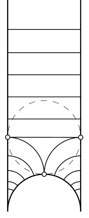
Figure 5: Horocycle foliation in a single ideal triangle.

We can endow the horocycle foliation with a transverse measure such that the measure of any geodesic arc $I$ contained in $\Delta$ is equal to its hyperbolic length. By collapsing each small unfoliated triangle to a 3-pronged singularity, we obtain a measured foliation in $\mathcal{MF}$.

This foliation is not compactly supported. However, the completeness of the hyperbolic metric guarantees that leaves near the cusped region must be closed. Thus we are able to obtain a compactly supported foliation by deleting all of these closed leaves paralleled to the punctures. Denote the resulted foliation by $\mathcal{F}_{\Delta}(X)$. See Figure 6 for an example of this process on $S_{1,2}$.

(a) An ideal triangulation of $S_{1,2}$ with the shear data.

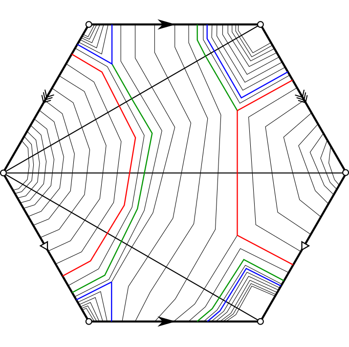
(b) The entire horocycle foliation, with colored singular leaves.

(c) The measured foliation $\mathcal{F}_{\Delta}(X)$. The boundary must consist of closed singular leaves.

Figure 6: From the shear data to a compactly supported measured foliation.

By [Thu86, Proposition 9.4] and [PaP93], the map

$$\mathcal{F}_{\Delta}:\mathcal{T}_{g,n} \longrightarrow\mathcal{MF}_{0}$$

$$X \mapsto\mathcal{F}_{\Delta}(X)$$

is a homeomorphism.

Denote the transverse measure of $\mathcal{F}_{\Delta}(X)$ on each edge $c\in\Delta$ by $m_{c}(X)$. We can embed $\mathcal{MF}_{0}$ into $\mathbb{R}_{\geq 0}^{6g-6+3n}$ as an Euclidean cone:

$$\mathcal{MF}_{0} \longrightarrow\mathbb{R}_{\geq 0}^{6g-6+3n}$$

$$\mathcal{F}_{\Delta}(X) \mapsto\left(m_{c_{i}}(X)\right)_{i=1}^{N}$$

We use the above map to define the symplectic form on $\mathcal{MF}_{0}$.

Proposition 5.1.

[PaP93, Corollary 4.2] The homeomorphism $\mathcal{F}_{\Delta}$ pulls back the Thurston’s symplectic form on $\mathcal{MF}_{0}$ to the Weil-Petersson form on $\mathcal{T}_{g,n}$.

Recall that $\mathcal{C}_{\Delta}$ is the image of the shearing coordinates, as a subspace of $\mathbb{R}^{6g-6+3n}$. By the above construction, we can consider the composition map $Sh_{\Delta}\circ\mathcal{F}_{\Delta}^{-1}$ as a map between Euclidean spaces. The following should be equivalent to [Thu86, Proposition 9.1].

Proposition 5.2.

The coordinate transformation $Sh_{\Delta}\circ\mathcal{F}_{\Delta}^{-1}$ from $\mathcal{MF}_{0}$ to $\mathcal{C}_{\Delta}$ is determined by

$$s_{e}(X)=\frac{1}{2}\bigg{(}m_{a}(X)+m_{c}(X)-m_{b}(X)-m_{d}(X)\bigg{)}$$

for each edge $e\in\Delta$. Here $a,b,e$ and $c,d,e$ are the edges of two adjacent ideal triangles, with $a,b,c,d$ in counterclockwise order.

Proof.

The formula follows immediately from the definition of shear and the construction of the measured foliation. See Figure 7. ∎

Figure 7: The measured foliation in a pair of adjacent ideal triangles.

A direct corollary is:

Theorem 5.3.

The Weil-Petersson volume form under the shearing coordinates is equal to the Euclidean volume form on $\mathcal{C}_{\Delta}$, up to a scaling constant.

5.2 Proof of Theorem 1.1

Proof.

It is obvious that the shear norm $\|Sh_{\Delta}\|$ is proper in $\mathcal{T}_{g,n}$. Applying Theorem 3.9 and Proposition 4.6 to Theorem 1.2, we have

$$\lim_{L\to+\infty}\frac{\#\left\{\ \phi\in\mathrm{Mod}_{g,n}\ \big{|}\ \|Sh_{\Delta}(\phi\cdot X)\|\leqslant L\ \right\}}{L^{6g-6+2n}}=\frac{n_{\Delta}\cdot B(X)}{b_{g,n}},$$

where

$$n_{\Delta}=\lim_{L\to+\infty}\frac{\mu_{wp}\left\{Y\in\mathcal{T}_{g,n}\ \big{|}\ \|Sh_{\Delta}(Y)\|\leqslant L\right\}}{L^{6g-6+2n}}\ .$$

We have shown in Theorem 5.3 that, up to a scaling constant, the Weil-Petersson volume form is equal to the Euclidean volume form on the image of the shearing coordinates, which is obviously homogenous. Thus the coefficient in (5.2) is equal to the volume of the unit ball. This finishes the proof.

∎

References

- [Ara20] Francisco Arana-Herrera, Counting hyperbolic multi-geodesics with respect to the lengths of individual components, arXiv:2002.10906 (2020).
- [Ara21] Francisco Arana-Herrera, Equidistribution of families of expanding horospheres on moduli spaces of hyperbolic surfaces, Geom. Dedicata 210 (2021), 65–102.
- [BBFS13] M. Bestvina, K. Bromberg, K. Fujiwara, And J. Souto, Shearing Coordinates And Convexity Of Length Functions On Teichmuller Space, Amer. J. Math. 135 (2013), no. 6, 1449–1476.
- [Bu] P. Buser, Geometry and spectra of compact Riemann surfaces, Birkhauser Boston, Boston, MA, 1992 (Reprinted in 2010).
- [ES19] Viveka Erlandsson, Juan Souto, Mirzakhani S Curve Counting (Research announcement), arXiv:1904.05091 (2019).
- [FLP] A. Fathi, F. Laudenbach, V. Poenaru, et al., Travaux de Thurston sur les surfaces, Astérisque, vol. 66–67, Société Mathématique de France, Paris, 1979.
- [FM] Benson Farb, Dan Margalit, A Primer on Mapping Class Groups, Princeton University Press, Princeton, NJ, 2012.
- [Hu] John H. Hubbard, Teichmüller Theory and Applications to Geometry, Topology, and Dynamics: Volume 1 Teichmiller Theory, Matrix Editions, Ithaca, NY, 2006.
- [Mir08] Maryam Mirzakhani, Growth of the number of simple closed geodesics on hyperbolic surfaces, Ann. of Math.(2), 168(1)(2008), 97–125.
- [Mir08b] Maryam Mirzakhani, Ergodic Theory of the Earthquake Flow, Int. Math. Res. Not. IMRN 2008, no. 3.
-
[Mir16]
Maryam Mirzakhani, Counting Mapping Class group orbits on hyperbolic surfaces,
arXiv:1601.03342 (2016). - [PaP93] A. Papadopoulos, R. C. Penner, The Weil-Petersson symplectic structure at Thurston’s boundary, Trans. Amer. Math. Soc. 335 (1993), no. 2, 891–904.
- [PeH] R. C. Penner, J. L. Harer, Combinatorics of Train Tracks, Annals of Mathematics Studies 125, Princeton University Press, Princeton, NJ, 1992.
- [SoB01] Yaşar Sözen, Francis Bonahon, The Weil-Petersson and Thurston symplectic forms, Duke Math. J. 108 (2001), no. 3, 581–597.
- [Thu86] William P. Thurston, Minimal stretch maps between hyperbolic surfaces, arxiv:9801039.
- [Wol82] Scott A. Wolpert, The Fenchel-Nielsen deformation, Ann. of Math.(2) 115 (1982), no. 3, 501–528.