Masked Conditional Random Fields for Sequence Labeling

Abstract

Conditional Random Field (CRF) based neural models are among the most performant methods for solving sequence labeling problems. Despite its great success, CRF has the shortcoming of occasionally generating illegal sequences of tags, e.g. sequences containing an “I-” tag immediately after an “O” tag, which is forbidden by the underlying BIO tagging scheme. In this work, we propose Masked Conditional Random Field (MCRF), an easy to implement variant of CRF that impose restrictions on candidate paths during both training and decoding phases. We show that the proposed method thoroughly resolves this issue and brings consistent improvement over existing CRF-based models with near zero additional cost.

1 Introduction

Sequence labeling problems such as named entity recognition (NER), part of speech (POS) tagging and chunking have long been considered as fundamental NLP tasks and drawn researcher’s attention for many years.

Traditional work is based on statistical approaches such as Hidden Markov Models (Baum and Petrie, 1966) and Conditional Random Fields (Lafferty et al., 2001), where handcrafted features and task-specific resources are used. With advances in deep learning, neural network based models have achieved dominance in sequence labeling tasks in an end-to-end manner. Those models typically consist of a neural encoder that maps the input tokens to embeddings capturing global sequence information, and a CRF layer that models dependencies between neighboring labels. Popular choices of neural encoder have been convolutional neural network (Collobert et al., 2011), and bidirectional LSTM (Huang et al., 2015). Recently, pretrained language models such as ELMo (Peters et al., 2018) or BERT (Devlin et al., 2019) have been proven far superior as a sequence encoder, achieving state-of-the-art results on a broad range of sequence labeling tasks.

Most sequence labeling models adopt a BIO or BIOES tag encoding scheme (Ratinov and Roth, 2009), which forbids certain tag transitions by design. Occasionally, a model may yield sequence of predicted tags that violates the rules of the scheme. Such predictions, subsequently referred to as illegal paths, are erroneous and must be dealt with. Existing methods rely on hand-crafted post-processing procedure to resolve this problem, typically by retaining the illegal segments and re-tagging them. But as we shall show in this work, such treatment is arbitrary and leads to suboptimal performance.

Dataset	legal & TP	illegal & TP	legal & FP	illegal & FP	$\frac{\textrm{illegal \& TP}}{\textrm{illegal}}$	$\frac{\textrm{illegal \& FP}}{\textrm{FP}}$	$\frac{\textrm{illegal}}{\textrm{total}}$
Resume	1445	1	68	17	1.4%	20%	1.2%
MSRA	5853	6	318	107	1.9%	25%	1.8%
Ontonotes	5323	5	1336	314	1.6%	19%	4.6%
Weibo	277	2	124	46	1.6%	27%	10.7%
ATIS	1643	0	70	24	0.0%	26%	1.4%
SNIPS	1542	13	237	156	5.2%	40%	8.7%
CoNLL2000	22957	36	888	100	3.9%	10%	0.6%
CoNLL2003	5131	2	535	74	0.4%	12%	1.3%

Table 1: Statistics of the predicted text segments by category over a variety of sequence labeling datasets. A BERT-CRF model with BIO scheme is trained for each of the dataset, and the statistics are computed on the respective dev set. When the model generates an illegal path, we determine the predicted segments as in (Sang et al., 2000), see Section 2.2 for more details. In the table “TP” and “FP” refer to “True Positive” and “False Positive” respectively. The column named “$\frac{\textrm{illegal \& TP}}{\textrm{illegal}}$” indicates the proportion of illegal segments that are correct predictions. The column named “$\frac{\textrm{illegal \& FP}}{\textrm{FP}}$” indicates the proportion of erroneous predictions that are due to illegal segments. The column named “$\frac{\textrm{illegal}}{\textrm{total}}$” stands for the proportion of illegal segments over all predictions.

The main contribution of this paper is to give a principled solution to the illegal path problem. More precisely:

1. We show that in the neural-CRF framework the illegal path problem is intrinsic and may accounts for non-negligible proportion (up to 40%) of total errors. To the best of our knowledge we are the first to conduct this kind of study.

2. We propose Masked Conditional Random Field (MCRF), an improved version of the CRF that is by design immune to the illegal paths problem. We also devise an algorithm for MCRF that requires only a few lines of code to implement.

3. We show in comprehensive experiments that MCRF performs significantly better than its CRF counterpart, and that its performance is on par with or better than more sophisticated models. Moreover, we achieve new State-of-the-Arts in two Chinese NER datasets.

The remainder of the paper is organized as follows. Section 2 describes the illegal path problem and existing strategies that resolve it. In Section 3 we propose MCRF, its motivation and an approximate implementation. Section 4 is devoted to numerical experiments. We conclude the current work in Section 5.

2 The illegal path problem

2.1 Problem Statement

As a common practice, most sequence labeling models utilize a certain tag encoding scheme to distinguish the boundary and the type of the text segments of interest. An encoding scheme makes it possible by introducing a set of tag prefixes and a set of tag transition rules. For instance, the popular BIO scheme distinguishes the Beginning, the Inside and the Outside of the chunks of interest, imposing that any I-$*$ tag must be preceded by a B-$*$ tag or another I-$*$ tag of the same type. Thus “O O O I-LOC I-LOC O” is a forbidden sequence of tags because the transition O $\to$ I-LOC directly violates the BIO scheme design. Hereafter we shall refer to a sequence of tags that contains at least one illegal transition an illegal path.

As another example, the BIOES scheme further identifies the Ending of the text segments and the Singleton segments, thereby introducing more transition restrictions than BIO. e.g. an I-$*$ tag must always be followed by an E-$*$ tag of the same type, and an S-$*$ tag can only be preceded by an O, an E-$*$ or another S-$*$ tag, etc. For a comparison of the performance of the encoding schemes, we refer to (Ratinov and Roth, 2009) and references therein.

When training a sequence labeling model with an encoding scheme, generally it is our hope that the model should be able to learn the semantics and the transition rules of the tags from the training data. However, even if the dataset is noiseless, a properly trained model may still occasionally make predictions that contains illegal transitions. This is especially the case for the CRF-based models, as there is no hard mechanism built-in to enforce those rules. The CRF ingredient by itself is only a soft mechanism that encourages legal transitions and penalizes illegal ones.

The hard transition rules might be violated when the model deems it necessary. To see this, let us consider a toy corpus where every occurrence of the token “America” is within the context of “North America”, thus the token is always labeled as I-LOC. Then, during training, the model may well establish the rule “America $\Rightarrow$ I-LOC” (Rule 1), among many other rules such as “an I-LOC tag does not follow an O tag” (Rule 2), etc. Now consider the test sample “Nathan left America last month”, which contains a stand-alone “America” labeled as B-LOC. During inference, as the model never saw a stand-alone “America” before, it must generalize. If the model is more confident on Rule 1 than Rule 2, then it may yield an illegal output “O O I-LOC O O”.

2.2 Strategies

The phenomenon of illegal path has already been noticed, but somehow regarded as trivial matters. For the BIO format, Sang et al. (2000) have stated that

The output of a chunk recognizer may contain inconsistencies in the chunk tags in case a word tagged I-X follows a word tagged O or I-Y, with X and Y being different. These inconsistencies can be resolved by assuming that such I-X tags starts a new chunk.

This simple strategy has been adopted by CoNLL-2000 as a standard post-processing procedure for the evaluation of the models’ performance, and gain its popularity ever since.

We argue that such treatment is not only arbitrary, but also suboptimal. In preliminary experiments we have studied the impact of the illegal path problem using the BERT-CRF model for a number of tasks and datasets. Our findings (see Table 1) suggest that although the illegal segments only account for a small fraction (typically around 1%) of total predicted segments, they constitute approximately a quarter of the false positives. Moreover, we found that only a few illegal segments are actually true positives. This raises the question of whether retaining the illegal segments is beneficial. As a matter of fact, as we will subsequently show, a much higher macro F1-score can be obtained if we simply discard every illegal segments.

Although the strategy of discarding the illegal segments may be superior to that of (Sang et al., 2000), it is nonetheless a hand-crafted, crude rule that lacks some flexibility. To see this, let us take the example in Fig. 1. The prediction for text segment World Boxing Council is (B-MISC, I-ORG, I-ORG), which contains an illegal transition B-MISC$\to$I-ORG. Clearly, neither of the post-processing strategies discussed above is capable of resolving the problem. Ideally, an optimal solution should convert the predicted tags to either (B-MISC, I-MISC, I-MISC) or (B-ORG, I-ORG, I-ORG), whichever is more likely. This is exactly the starting point of MCRF, which we introduce in the next section.

3 Approach

Figure 1: An example of CRF decoded path vs. MCRF decoded path. The CRF decoded path is represented as black arrows in the figure. This path contains one illegal transition (black dashed arrow) B-MISC$\to$I-ORG, which results in two erroneous predictions: MISC for “World” and ORG for “Boxing Council”. When using MCRF instead, the decoding algorithm has to search for an alternative path (red arrows), as all illegal transitions are blocked. In this example, MCRF correctly predicts MISC for the entity “World Boxing Council”.

In this section we introduce the motivation and implementation of MCRF. We first go over the conventional neural-based CRF models in Section 3.1. We then introduce MCRF in Section 3.2. Its implementation will be given in Section 3.3.

3.1 Neural CRF Models

Conventional neural CRF models typically consist of a neural network and a CRF layer. The neural network component serves as an encoder that usually first maps the input sequence of tokens to a sequence of token encodings, which is then transformed (e.g. via a linear layer) into a sequence of token logits. Each logit therein models the emission scores of the underlying token. The CRF component introduces a transition matrix that models the transition score from tag $i$ to tag $j$ for any two consecutive tokens. By aggregating the emission scores and the transition scores, deep CRF models assign a score for each possible sequence of tags.

Before going any further, let us introduce some notations first. In the sequel, we denote by $x=\{x_{1},x_{2},\ldots,x_{T}\}$ a sequence of input tokens, by $y=\{y_{1},\ldots,y_{T}\}$ their ground truth tags and by $l=\{l_{1},\ldots,l_{T}\}$ the logits generated by the encoder network of the model. Let $d$ be the number of distinct tags and denote by $[d]:=\{1,\ldots,d\}$ the set of tag indices. Then $y_{i}\in[d]$ and $l_{i}\in\mathbb{R}^{d}$ for $1\leq i\leq T$. We denote by $W$ the set of all trainable weights in the encoder network, and by $A=(a_{ij})\in\mathbb{R}^{d\times d}$ the transition matrix introduced by the CRF, where $a_{ij}$ is the transition score from tag $i$ to tag $j$. For convenience we call a sequence of tags a path. For given input $x$, encoder weights $W$ and transition matrix $A$, we define the score of a path $p=\{n_{1},\ldots,n_{T}\}$as

$$\halign to=0.0pt{\relax\global\advance\@IEEEeqncolcnt by 1\relax\begingroup\csname @IEEEeqnarraycolPREr\endcsname#\relax\relax\relax\relax\relax\relax\relax\relax\relax\relax\csname @IEEEeqnarraycolPOSTr\endcsname\relax\relax\relax\relax\relax\relax\relax\relax\relax\relax\endgroup&\relax\global\advance\@IEEEeqncolcnt by 1\relax\begingroup\csname @IEEEeqnarraycolPREC\endcsname#\relax\relax\relax\relax\relax\relax\relax\relax\relax\relax\csname @IEEEeqnarraycolPOSTC\endcsname\relax\relax\relax\relax\relax\relax\relax\relax\relax\relax\endgroup&\relax\global\advance\@IEEEeqncolcnt by 1\relax\begingroup\csname @IEEEeqnarraycolPREl\endcsname#\relax\relax\relax\relax\relax\relax\relax\relax\relax\relax\csname @IEEEeqnarraycolPOSTl\endcsname\relax\relax\relax\relax\relax\relax\relax\relax\relax\relax\endgroup&\global\advance\@IEEEeqncolcnt by 1\relax\bgroup#\egroup&\global\advance\@IEEEeqncolcnt by 1\relax\hbox to\z@\bgroup\hss#\egroup\cr\hfil$\displaystyle s(p, x, W, A) = \sum_{i=1}^{T} l_{i, n_{i}} + \sum_{i=1}^{T-1} a_{n_{i}, n_{i+1}} , $&\hfil$\displaystyle{}{}$\hfil&$\displaystyle$\hfil&{\vrule width=0.0pt,height=0.0pt,depth=0.0pt}&0.0pt{\hss{\normalcolor(1)}}\cr}$$

where $l_{i,j}$ denotes the $j$-th entry of $l_{i}$. Let $\mathcal{S}$ be the set of all training samples, and $\mathcal{P}$ be the set of all possible paths. Then the loss function of neural CRF model is the average of negative log-likelihood over $\mathcal{S}$:

$$\mathcal{L}(W,A)=-\frac{1}{|\mathcal{S}|}\!\!\sum_{(x,y)\in\mathcal{S}}\!\!\!\log\frac{\exp{s(y,x)}}{\sum_{p\in\mathcal{P}}\exp{s(p,x)}}$$ (2)

where we have omitted the dependence of $s(\cdot,\cdot)$ on $(W,A)$ for conciseness. One can easily minimize $\mathcal{L}(W,A)$ using any popular first-order methods such as SGD or Adam.

Let $(W_{\textrm{opt}},A_{\textrm{opt}})$ be a minimizer of $\mathcal{L}$. During decoding phase, the predicted path for a test sample $x_{\textrm{test}}$ is the path having the highest score, i.e.

$$y_{\textrm{opt}}=\underset{p\in\mathcal{P}}{\operatorname{argmax\,\,}}s(p,x_{\textrm{test}},W_{\textrm{opt}},A_{\textrm{opt}}).$$ (3)

The decoding problem can be efficiently solved by the Viterbi algorithm.

3.2 Masked CRF

Our major concern on conventional neural CRF models is that no hard mechanism exists to enforce the transition rule, resulting in occasional occurrence of illegal predictions.

Our solution to this problem is very simple. Denote by $\mathcal{I}$ the set of all illegal paths. We propose to constrain the “path space” in the CRF model to the space of all legal paths $\mathcal{P}/\mathcal{I}$, instead of the entire space of all possible paths $\mathcal{P}$. To this end,

1. during training, the normalization term in (2) should be the sum of the exponential scores of the legal paths;

2. during decoding, the optimal path should be searched over the space of all legal paths.

The first modification above leads to the following new loss function:

$$\mathcal{L}^{\prime}(W,A)\!\!\!\! := \!\!\!\!-\frac{1}{|\mathcal{S}|}\!\!\sum_{(x,y)\in\mathcal{S}}\!\!\!\log\frac{\exp{s(y,x)}}{\sum_{p\in\mathcal{P}/\mathcal{I}}\exp{s(p,x)}},$$

which is obtained by replacing the $\mathcal{P}$ in (2) by $\mathcal{P}/\mathcal{I}$.

Similarly, the second modification leads to

$$\halign to=0.0pt{\relax\global\advance\@IEEEeqncolcnt by 1\relax\begingroup\csname @IEEEeqnarraycolPREr\endcsname#\relax\relax\relax\relax\relax\relax\relax\relax\relax\relax\csname @IEEEeqnarraycolPOSTr\endcsname\relax\relax\relax\relax\relax\relax\relax\relax\relax\relax\endgroup&\relax\global\advance\@IEEEeqncolcnt by 1\relax\begingroup\csname @IEEEeqnarraycolPREC\endcsname#\relax\relax\relax\relax\relax\relax\relax\relax\relax\relax\csname @IEEEeqnarraycolPOSTC\endcsname\relax\relax\relax\relax\relax\relax\relax\relax\relax\relax\endgroup&\relax\global\advance\@IEEEeqncolcnt by 1\relax\begingroup\csname @IEEEeqnarraycolPREl\endcsname#\relax\relax\relax\relax\relax\relax\relax\relax\relax\relax\csname @IEEEeqnarraycolPOSTl\endcsname\relax\relax\relax\relax\relax\relax\relax\relax\relax\relax\endgroup&\global\advance\@IEEEeqncolcnt by 1\relax\bgroup#\egroup&\global\advance\@IEEEeqncolcnt by 1\relax\hbox to\z@\bgroup\hss#\egroup\cr\hfil$\displaystyle y'_{\mathrm{opt}} = \underset{p\in\mathcal{P}/ \mathcal{I}}{\operatorname{argmax\,\,}} s(p, x_{\mathrm{test}}, W_{\mathrm{opt}}', A_{\mathrm{opt}}') $&\hfil$\displaystyle{}{}$\hfil&$\displaystyle$\hfil&{\vrule width=0.0pt,height=0.0pt,depth=0.0pt}&0.0pt{\hss{\normalcolor(5)}}\cr}$$

obtained by replacing the $\mathcal{P}$ in (3) by $\mathcal{P}/\mathcal{I}$, where $(W_{\textrm{opt}}^{\prime},A_{\textrm{opt}}^{\prime})$ is a minimizer of (LABEL:mcrfloss).

Note that the decoding objective (3.2) alone is enough to guarantee the complete elimination of illegal paths. However, this would create a mismatch between the training and the inference, as the model would attribute non-zero probability mass to the ensemble of the illegal paths. In Section 4.1, we will see that a naive solution based on (3.2) alone leads to suboptimal performance compared to a proper solution based on both (LABEL:mcrfloss) and (3.2).

3.3 Algorithm

Figure 2: An example of the masked transition matrix under the BIO scheme. The entries in the red cells are masked as they correspond to illegal transitions. Under the BIO scheme, there are two types of illegal transitions: O $\to$ I-X for any X and B-X $\to$ I-Y for any X, Y such that X $\neq$ Y.

Although in principle it is possible to directly minimize (LABEL:mcrfloss), thanks to the following proposition we can also achieve this via reusing the existing tools originally designed for minimizing (2), thereby saving us from making extra engineering efforts.

Proposition 1.

Denote by $\Omega\subset[d]\times[d]$ the set of all illegal transitions. For a given transition matrix $\mathbf{A}$, we denote by $\bar{A}(c)=\big{(}\bar{a}_{ij}(c)\big{)}$ the masked transition matrix of $A$ defined as (see Fig. 2)

$$\bar{a}_{ij}(c)=\left\{\begin{array}[]{ll}c&\textrm{if }(i,j)\in\Omega,\\ a_{ij}&\textrm{otherwise},\end{array}\right.$$ (8)

where $c\ll 0$ is the transition mask. Then for arbitrary model weights $(W_{0},A_{0})$, we have

$$\halign to=0.0pt{\relax\global\advance\@IEEEeqncolcnt by 1\relax\begingroup\csname @IEEEeqnarraycolPREr\endcsname#\relax\relax\relax\relax\relax\relax\relax\relax\relax\relax\csname @IEEEeqnarraycolPOSTr\endcsname\relax\relax\relax\relax\relax\relax\relax\relax\relax\relax\endgroup&\relax\global\advance\@IEEEeqncolcnt by 1\relax\begingroup\csname @IEEEeqnarraycolPREC\endcsname#\relax\relax\relax\relax\relax\relax\relax\relax\relax\relax\csname @IEEEeqnarraycolPOSTC\endcsname\relax\relax\relax\relax\relax\relax\relax\relax\relax\relax\endgroup&\relax\global\advance\@IEEEeqncolcnt by 1\relax\begingroup\csname @IEEEeqnarraycolPREl\endcsname#\relax\relax\relax\relax\relax\relax\relax\relax\relax\relax\csname @IEEEeqnarraycolPOSTl\endcsname\relax\relax\relax\relax\relax\relax\relax\relax\relax\relax\endgroup&\global\advance\@IEEEeqncolcnt by 1\relax\bgroup#\egroup&\global\advance\@IEEEeqncolcnt by 1\relax\hbox to\z@\bgroup\hss#\egroup\cr\hfil$\displaystyle\lim_{c\to- \infty} \mathcal{L}(W_{0}, \bar{A}_{0}(c)) $&\hfil$\displaystyle{}= {}$\hfil&$\displaystyle\mathcal{L}'(W_{0}, A_{0}) $\hfil&{{}\vrule width=0.0pt,height=0.0pt,depth=0.0pt}&0.0pt{\hss{\normalcolor(9)}}\cr\penalty 100\vskip 3.0pt\vskip 0.0pt\cr\hfil$\displaystyle\!\!\!\!\!\!\!\!\! \lim_{c\to- \infty}\!\! \nabla_{W} \mathcal{L}(W_{0}, \bar{A}_{0}(c)) $&\hfil$\displaystyle{}= {}$\hfil&$\displaystyle\nabla_{W} \mathcal{L}'(W_{0}, A_{0}) $\hfil&{\vrule width=0.0pt,height=0.0pt,depth=0.0pt}&0.0pt{\hss{\normalcolor(10)}}\cr}$$

and for all $(i,j)\in\Omega$

$$\halign to=0.0pt{\relax\global\advance\@IEEEeqncolcnt by 1\relax\begingroup\csname @IEEEeqnarraycolPREr\endcsname#\relax\relax\relax\relax\relax\relax\relax\relax\relax\relax\csname @IEEEeqnarraycolPOSTr\endcsname\relax\relax\relax\relax\relax\relax\relax\relax\relax\relax\endgroup&\relax\global\advance\@IEEEeqncolcnt by 1\relax\begingroup\csname @IEEEeqnarraycolPREC\endcsname#\relax\relax\relax\relax\relax\relax\relax\relax\relax\relax\csname @IEEEeqnarraycolPOSTC\endcsname\relax\relax\relax\relax\relax\relax\relax\relax\relax\relax\endgroup&\relax\global\advance\@IEEEeqncolcnt by 1\relax\begingroup\csname @IEEEeqnarraycolPREl\endcsname#\relax\relax\relax\relax\relax\relax\relax\relax\relax\relax\csname @IEEEeqnarraycolPOSTl\endcsname\relax\relax\relax\relax\relax\relax\relax\relax\relax\relax\endgroup&\global\advance\@IEEEeqncolcnt by 1\relax\bgroup#\egroup&\global\advance\@IEEEeqncolcnt by 1\relax\hbox to\z@\bgroup\hss#\egroup\cr\hfil$\displaystyle\!\!\!\!\!\!\!\!\!\!\!\! \lim_{c\to- \infty}\!\! \nabla_{a_{ij}} \mathcal{L}(W_{0}, \bar{A}_{0}(c)) = \nabla_{a_{ij}} \mathcal{L}'(W_{0}, A_{0}). $&\hfil$\displaystyle{}{}$\hfil&$\displaystyle$\hfil&{\vrule width=0.0pt,height=0.0pt,depth=0.0pt}&0.0pt{\hss{\normalcolor(11)}}\cr}$$

Moreover, for negatively large enough $c$ we have

$$\halign to=0.0pt{\relax\global\advance\@IEEEeqncolcnt by 1\relax\begingroup\csname @IEEEeqnarraycolPREr\endcsname#\relax\relax\relax\relax\relax\relax\relax\relax\relax\relax\csname @IEEEeqnarraycolPOSTr\endcsname\relax\relax\relax\relax\relax\relax\relax\relax\relax\relax\endgroup&\relax\global\advance\@IEEEeqncolcnt by 1\relax\begingroup\csname @IEEEeqnarraycolPREC\endcsname#\relax\relax\relax\relax\relax\relax\relax\relax\relax\relax\csname @IEEEeqnarraycolPOSTC\endcsname\relax\relax\relax\relax\relax\relax\relax\relax\relax\relax\endgroup&\relax\global\advance\@IEEEeqncolcnt by 1\relax\begingroup\csname @IEEEeqnarraycolPREl\endcsname#\relax\relax\relax\relax\relax\relax\relax\relax\relax\relax\csname @IEEEeqnarraycolPOSTl\endcsname\relax\relax\relax\relax\relax\relax\relax\relax\relax\relax\endgroup&\global\advance\@IEEEeqncolcnt by 1\relax\bgroup#\egroup&\global\advance\@IEEEeqncolcnt by 1\relax\hbox to\z@\bgroup\hss#\egroup\cr\hfil$\displaystyle\underset{p\in\mathcal{P}}{\operatorname{argmax\,\,}} s(p, x_{{test}}, W, A) = \underset{p\in\mathcal{P}/\mathcal{I}}{\operatorname{argmax\,\,}} s(p, x_{{test}}, W, A) $&\hfil$\displaystyle{}{}$\hfil&$\displaystyle$\hfil&{\vrule width=0.0pt,height=0.0pt,depth=0.0pt}&0.0pt{\hss}\cr}$$

Proof. See Appendix.

Proposition 1 states that for any given model state $(W,A)$, if we mask the entries of $A$ that correspond to illegal transitions (see Figure 2) by a negatively large enough constant $c$, then the two objectives (2) and (LABEL:mcrfloss), as well as their gradients, can be arbitrarily close. This suggests that the task of minimizing (LABEL:mcrfloss) can be achieved via minimizing (2) combined with keeping $A$ masked (i.e. making $a_{ij}=c$ constant for all $(i,j)\in\Omega$) throughout the optimization process.

Intuitively, the purpose of transition masking is to penalize the illegal transitions in such a way that they will never be selected during the Viterbi decoding, and the illegal paths as a whole only constitutes negligible probability mass during training.

Based on Proposition 1, we propose the Masked CRF approach, formally described in Algorithm 1.

Algorithm 1 (MCRF)

1:Input: Library for computing the gradients of conventional CRF loss (2), training dataset $\mathcal{S}$, stopping criterion $\mathcal{C}$, set of illegal transitions $\Omega$, masking constant $c\ll 0$.

2:Initialize: model weight $W$ and tag transition matrix $A=(a_{ij})$.

3:while $\mathcal{C}$ is not met do

4:     Sample a mini-batch from $\mathcal{S}$

5:     Update $W$ and $A$ based on batch gradient

6:     for $(i,j)\in\Omega$ do

7:         $a_{ij}\leftarrow c$ $\triangleright$ maintain the mask

8:     end for

9:end while

10:Output: Optimized $W$ and $A$.

4 Experiments

In this section, we run a series of experiments to evaluate the performance of MCRF. The datasets used in our experiments are listed as follows:

• Chinese NER: OntoNotes 4.0 (Weischedel et al., 2011), MSRA (Levow, 2006), Weibo (Peng and Dredze, 2015) and Resume (Zhang and Yang, 2018).

• English NER: CoNLL2003 (Tjong Kim Sang and De Meulder, 2003)

• Slot Filling: ATIS (Hemphill et al., 1990) and SNIPS (Coucke et al., 2018)

• Chunking: CoNLL2000 (Sang et al., 2000)

The statistics of these datasets are summarized in Table 2.

dataset	task	lan.	labels	train	dev	test
Resume	NER	CN	8	3.8k	472	477
MSRA	NER	CN	3	46.3k	-	4.3k
Ontonotes	NER	CN	4	15.7k	4.3k	4.3k
Weibo	NER	CN	7	1.3k	270	270
ATIS	SF	EN	79	4.5k	500	893
SNIPS	SF	EN	39	13.0k	700	700
CoNLL2000	Chunk.	EN	11	8.9k	-	2.0k
CoNLL2003	NER	EN	4	14.0k	3.2k	3.5k

Table 2: Statistics of the datasets.

For Chinese NER tasks, we use the public-available $\textrm{BERT}_{\textrm{BASE}}$ as the pretrained model. For English NER and Chunking tasks, we use the cased version of $\textrm{BERT}_{\textrm{BASE}}$ model. We use uncased $\textrm{BERT}_{\textrm{BASE}}$ for English slot filling tasks.

	Resume	MSRA	Ontonotes	Weibo
Lattice (Zhang and Yang, 2018)	94.5	93.2	73.9	58.8
Glyce (Meng et al., 2019)†	96.5	95.5	81.6	67.6
SoftLexicon (Ma et al., 2020)†	96.1	95.4	82.8	70.5
FLAT (Li et al., 2020a)†	95.9	96.1	81.8	68.6
MRC (Li et al., 2020b)†	-	95.7	82.1	-
DSC (Li et al., 2020c)†	-	96.7	84.5	-
BERT-tagger-retain	95.7 (94.7)	94.0 (92.7)	78.1 (76.8)	67.7 (65.3)
BERT-tagger-discard	96.2 (95.5)	94.6 (93.6)	80.7 (79.2)	69.7 (67.5)
BERT-CRF-retain	95.9 (94.8)	94.2 (93.7)	81.8 (81.2)	70.8 (64.5)
BERT-CRF-discard	97.2 (96.6)	95.5 (94.9)	83.1 (82.4)	71.9 (65.7)
BERT-MCRF-decoding	97.3 (96.6)	95.6 (95.0)	83.2 (82.5)	72.2 (65.8)
BERT-MCRF-training	97.6 (96.9)	95.9 (95.3)	83.7 (82.7)	72.4 (66.5)

Table 3: Results on Chinese NER datasets. The “$\dagger$” symbol implies that the reported result is based on BERT. The numbers in the parenthesis and the numbers next to it indicate the average and max F1-score, respectively.

In preliminary experiments, we found out that the discriminative fine-tuning approach (Howard and Ruder, 2018) yields slightly better results than the standard fine-tuning as recommended by (Devlin et al., 2019). In discriminative fine-tuning, one uses different learning rates for each layer. Let $r_{L}$ be the learning rate for the last ($L$-th) layer and $\eta$ be the decay factor. Then the learning rate for the $(L-n)$-th layer is given by $r_{L-n}=r_{L}\eta^{n}$. In our experiments, we use $r_{L}\in\{1e-4,5e-5\}$ and $\eta\in\{1/2,2/3\}$ depending on the dataset. The standard Adam optimizer is used throughout, and the mini-batch size is fixed to be 32. We always fine-tune for 5 epochs or 10000 iterations, whichever is longer.

4.1 Main results

In this section we present the MCRF results on 8 sequence labeling datasets. The baseline models are the following:

• BERT-tagger: The output of the final hidden representation for to each token is fed into a classification layer over the label set without using CRF. This is the approach recommended in (Devlin et al., 2019).

• BERT-CRF: BERT followed by a CRF layer, as is described in Section 3.1.

We use the following strategies to handle the illegal segments (See Table 4 for an example):

• retain: Keep and retag the illegal segments. This strategy agrees with (Sang et al., 2000).

• discard: Discard the illegal segments completely.

original:	O	I-PER	O	B-LOC	I-MISC
retain:	O	B-PER	O	B-LOC	B-MISC
discard:	O	O	O	B-LOC	O

Table 4: An example illustrating the difference between “retain” strategy and “discard” strategy.

We distinguish two versions of MCRF:

• MCRF-decoding: A naive version of MCRF that does masking only in decoding. The training process is the same as that in conventional CRF.

• MCRF-training: The proper MCRF approach proposed in this work. The masking is maintained in the training, as is described in Section 3.3. We also refer to it as the MCRF for simplicity.

For each dataset and each model we ran the training 10 times with different random initializations and selected the model that performed best on the dev set for each run. We report the best and the average test F1-scores as the final results. If the dataset does not provide an official development set, we randomly split the training set and use 10% of the samples as the dev set.

4.1.1 Results on Chinese NER

The results on Chinese NER tasks are presented in Table 3. It can be seen that the MCRF-training approach significantly outperforms all baseline models and establishes new State-of-the-Arts for Resume and Weibo datasets. From these results we can assert that the improvement brought by MCRF is mainly due to the effect of masking in training, not in decoding. Besides, we notice that the “discard” strategy substantially outperforms the “retain” strategy, which agrees with the statistics presented in Table 1.

We also plotted in Fig. 3 the loss curves of CRF and MCRF on the development set of MSRA. It can be clearly seen that MCRF incurs a much lower loss during training. This confirms our hypothesis that the CRF model attributes non-zero probability mass to the ensemble of the illegal paths, as otherwise the denominators in (LABEL:mcrfloss) and in (2) would have been equal, and in that case the loss curves of CRF and MCRF would have converged to the same level.

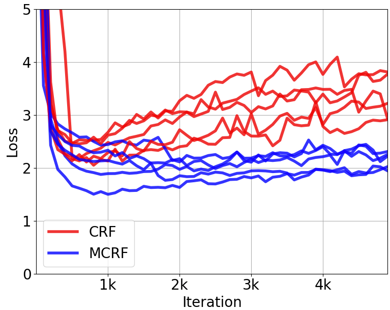
Figure 3: Curves of dev loss for CRF and MCRF.

Note that some of the results listed in Table 3 are based on models that utilize additional resources. Zhang and Yang (2018) and Ma et al. (2020) utilized Chinese lexicon features to enrich the token representations. Meng et al. (2019) combined Chinese glyph information with BERT pre-training. In contrast, the proposed MCRF approach is simple yet performant. It achieves comparable or better results without relying on additional resources.

4.1.2 Results on Slot Filling

One of the main features of the AITS and SNIPS datasets is the large number of slot labels (79 and 39 respectively) with relatively small training set (4.5k and 13k respectively). This requires the sequence labeling model learn the transition rules in a sample-efficient manner. Both ATIS and SNIPS provide an intent label for each utterance in the datasets, but in our experiments we did not use this information and rely solely on the slot labels.

The results are reported in Table 5. It can be seen that MCRF-training outperforms the baseline models and achieves competitive results compared to previous published results.

Model	ATIS	SNIPS
(Goo et al., 2018)	95.4	89.3
(Li et al., 2018)	96.5	-
(Zhang et al., 2019)	95.2	91.8
(E et al., 2019)	95.8	92.2
(Siddhant et al., 2019)	95.6	93.9
BERT-tagger-retain	95.2 (92.9)	93.2 (92.1)
BERT-tagger-discard	95.6 (93.1)	93.5 (92.3)
BERT-CRF-retain	95.5 (93.5)	94.6 (93.7)
BERT-CRF-discard	95.8 (93.9)	95.1 (94.3)
BERT-MCRF-decoding	95.8 (93.9)	95.1 (94.4)
BERT-MCRF-training	95.9 (94.4)	95.3 (94.6)

Table 5: Test F1-scores on slot filling datasets.

4.1.3 Results on Chunking

The results on CoNLL2000 chunking task are reported in Table. 6. The proposed MCRF-training outperforms the CRF baseline by 0.4 in F1-score.

Model	F1
ELMo (Peters et al., 2017)	96.4
CSE (Akbik et al., 2018)	96.7
GCDT (Liu et al., 2019)	97.3
BERT-tagger-retain	96.1 (95.7)
BERT-tagger-discard	96.3 (96.0)
BERT-CRF-retain	96.5 (96.2)
BERT-CRF-discard	96.6 (96.3)
BERT-MCRF-decoding	96.6 (96.4)
BERT-MCRF-training	96.9 (96.5)

Table 6: Results on CoNLL2000 chunking task.

4.2 Ablation Studies

In this section, we investigate the influence of various factors that may impact the performance of MCRF. In particular, we are interested in the quantity MCRF gain, which we denote by $\Delta$, defined simple as the difference of F1-score of MCRF-training and that of the conventional CRF (with either “retain” or “discard” strategy).

4.2.1 Effect of Tagging Scheme

In the previous experiments we have always used the BIO scheme. It is of interest to explore the performance of MCRF under other tagging schemes such as BIOES. The BIOES scheme is considered more expressive than BIO as it introduces more labels and more transition restrictions.

We have re-run the experiments in Section 4.1.1 using the BIOES scheme. Our results are reported in Fig. 4 and Table 7. It is clearly seen that under the BIOES scheme MCRF still always outperforms the CRF baselines. Note that compared to the case under BIO scheme, the MCRF gain is less significant against the CRF-retain baseline, but larger against CRF-discard.

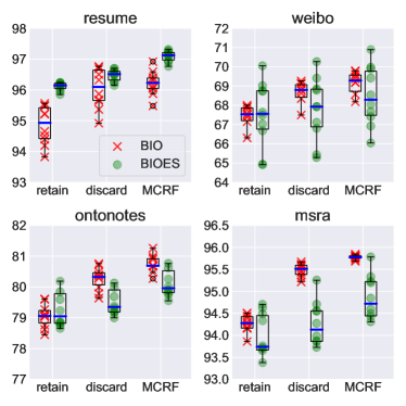
Figure 4: Ablation over the tagging scheme (BIO vs. BIOES). The F1-scores on the dev sets are plotted.

	BIO		BIOES
	$\Delta_{\textrm{ret.}}$	$\Delta_{\textrm{disc.}}$	$\Delta_{\textrm{ret.}}$	$\Delta_{\textrm{disc.}}$
Resume	2.1	0.3	1.0	0.6
MSRA	1.6	0.4	0.8	0.6
Ontonotes	1.5	0.3	0.9	0.6
Weibo	2.0	0.8	0.9	0.8

Table 7: A comparison of the average MCRF gain under BIO and BIOES schemes. The symbols $\Delta_{\textrm{ret.}}$ and $\Delta_{\textrm{disc.}}$ stand for the gain against BERT-retain and BERT-discard, respectively.

4.2.2 Effect of Sample Size

One may hypothesize that the occurrence of illegal paths might be due to the scarcity of training data, i.e. a model should be less prone to illegal paths if the training dataset is larger. To test this hypothesis, we randomly sample 10% of the training data from MSRA and Ontonotes, creating a smaller version of the respective dataset. We compare the proportion of the illegal segments produced by BERT-CRF trained on the original dataset with the one trained on the smaller dataset. We also report the performance gain brought by MCRF in these two scenarios. Our findings are summarized in Table 8. As can be seen from the table, the models trained with fewer data do yield slightly more illegal segments, but the MCRF gains under the two scenarios are close.

	MSRA-full			MSRA-10%
	ill.	F1	$\Delta$	ill.	F1	$\Delta$
retain	1.8%	94.2	1.6	2.4%	90.4	1.2
discard	-	95.4	0.5	-	90.7	0.9
MCRF	0%	95.8	-	0%	91.6	-
	Ontonotes-full			Ontonotes-10%
	ill.	F1	$\Delta$	ill.	F1	$\Delta$
retain	4.2%	79.2	1.6	4.7%	78.7	1.2
discard	-	80.4	0.4	-	79.1	0.8
MCRF	0%	80.8	-	0%	79.9	-

Table 8: Ablation over the training set size. The column named “ill.” indicates the proportion of illegal segments over all predicted segments.

4.2.3 Effect of Encoder Architecture

So far we have experimented with BERT-based models. Now we explore effect of neural architecture. We trained a number of models on CoNLL2003 with varying encoder architectures. The key components are listed as follows:

• ELMo: pretrained language model that serves as an sequence encoder.

• CNN: CNN-based character embedding layer, with weights extracted from pretrained ELMo. It is used to generate word embeddings for arbitrary input tokens.

• LSTM-$n$: $n$-layer bidirectional LSTM with hidden dimension $h=200$.

The results of our experiments are given in Table 9. We observe that the encoder architecture has a large impact on the occurrence of illegal paths, and the BERT-based models appear to generate much more illegal paths than ELMo-based ones. This is probably due to the fact that transformer-encoders are not sequential in nature. A further study is needed to investigate this phenomenon, but it is beyond the scope of the current work. We also notice that the MCRF gain seems to be positively correlated with the proportion of the illegal paths generated by the underlying model. This is expected, since the transition-blocking mechanism of MCRF will (almost) not take effect if the most probable path estimated by the underlying CRF model is already legal.

Encoder	ill.	err.	CRF	MCRF	$\Delta$
LSTM-1	3.1%	11.7%	82.2	83.2	1.0
LSTM-2	1.4%	8.3%	84.3	85.1	0.8
CNN + LSTM-1	0.4%	4.0%	94.1	94.3	0.2
CNN + LSTM-2	0.3%	2.3%	94.0	94.5	0.5
ELMo + LSTM-1	0.4%	3.3%	95.1	95.3	0.2
ELMo + LSTM-2	0.6%	5.5%	95.0	95.3	0.3
BERT	1.3%	12.5%	94.5	95.4	0.9
BERT + LSTM-1	1.0%	13.1%	94.7	95.3	0.6
BERT + LSTM-2	0.9%	10.3%	93.9	95.0	1.1

Table 9: Ablation over the encoder models. The column named “err.” indicates the proportion of erroneous predictions that are due to illegal segments.

4.3 Related Work

Some models are able to solve sequence labeling tasks without relying on BIO/BIOES type of tagging scheme to distinguish the boundary and the type of the text segments of interest, thus do not suffer from the illegal path problems. For instance, Semi-Markov CRF (Sarawagi and Cohen, 2005) uses an additional loop to search for the segment spans, and directly yields a sequence of segments along with their type. The downside of Semi-Markov CRF is that it incurs a higher time complexity compared to the conventional CRF approach. Recently, Li et al. (2020b) proposed a Machine Learning Comprehension (MRC) framework to solve NER tasks. Their model uses two separate binary classifiers to predict whether each token is the start or end of an entity, and an additional module to determine which start and end tokens should be matched.

We notice that the CRF implemented in PyTorch-Struct (Rush, 2020) has a different interface than usual CRF libraries and it takes not two tensors for emission and transition scores, but rather one score tensor of the shape (batch size, sentence length, number of tags, number of tags). This allows one to incorporate even more prior knowledge in the structured prediction by setting a constraint mask as a function of not only a pair of tags, but also words on which the tags are assigned. Such feature may be exploited in future work.

Finally, we acknowledge that the naive version of MCRF that does constrained decoding has already been implemented in AllenNLP (Gardner et al., 2018). As shown in Section 4.1, such approach is suboptimal compared to the proposed MCRF-training method.

5 Conclusion

Our major contribution is the proposal of MCRF, a constrained variant of CRF that masks illegal transitions during CRF training, eliminating illegal outcomes in a principled way.

We have justified MCRF from a theoretical perspective, and shown empirically in a number of datasets that MCRF consistently outperforms the conventional CRF. As MCRF is easy to implement and incurs zero additional overhead, we advocate always using MCRF instead of CRF when applicable.

Appendix A Appendices

A.1 Proof of Proposition 1

Denote by $L$ and $L^{\prime}$ the likelihood function of sample $(x,y)$ for CRF and MCRF model respectively:

$$\halign to=0.0pt{\relax\global\advance\@IEEEeqncolcnt by 1\relax\begingroup\csname @IEEEeqnarraycolPREr\endcsname#\relax\relax\relax\relax\relax\relax\relax\relax\relax\relax\csname @IEEEeqnarraycolPOSTr\endcsname\relax\relax\relax\relax\relax\relax\relax\relax\relax\relax\endgroup&\relax\global\advance\@IEEEeqncolcnt by 1\relax\begingroup\csname @IEEEeqnarraycolPREC\endcsname#\relax\relax\relax\relax\relax\relax\relax\relax\relax\relax\csname @IEEEeqnarraycolPOSTC\endcsname\relax\relax\relax\relax\relax\relax\relax\relax\relax\relax\endgroup&\relax\global\advance\@IEEEeqncolcnt by 1\relax\begingroup\csname @IEEEeqnarraycolPREl\endcsname#\relax\relax\relax\relax\relax\relax\relax\relax\relax\relax\csname @IEEEeqnarraycolPOSTl\endcsname\relax\relax\relax\relax\relax\relax\relax\relax\relax\relax\endgroup&\global\advance\@IEEEeqncolcnt by 1\relax\bgroup#\egroup&\global\advance\@IEEEeqncolcnt by 1\relax\hbox to\z@\bgroup\hss#\egroup\cr\hfil$\displaystyle L(W, A) $&\hfil$\displaystyle{}= {}$\hfil&$\displaystyle\frac{\exp{s(y, x, W, A)}}{\sum_{p\in\mathcal{P}} \exp{s(p, x, W, A)}}, $\hfil&{{}\vrule width=0.0pt,height=0.0pt,depth=0.0pt}&0.0pt{\hss{\normalcolor(12)}}\cr\penalty 100\vskip 3.0pt\vskip 0.0pt\cr\hfil$\displaystyle L'(W, A) $&\hfil$\displaystyle{}= {}$\hfil&$\displaystyle\frac{\exp{s(y, x, W, A)}}{\sum_{p\in\mathcal{P}/\mathcal{I}} \exp{s(p, x, W, A)}} . $\hfil&{\vrule width=0.0pt,height=0.0pt,depth=0.0pt}&0.0pt{\hss{\normalcolor(13)}}\cr}$$

To simplify the notations, we also write

$$\halign to=0.0pt{\relax\global\advance\@IEEEeqncolcnt by 1\relax\begingroup\csname @IEEEeqnarraycolPREr\endcsname#\relax\relax\relax\relax\relax\relax\relax\relax\relax\relax\csname @IEEEeqnarraycolPOSTr\endcsname\relax\relax\relax\relax\relax\relax\relax\relax\relax\relax\endgroup&\relax\global\advance\@IEEEeqncolcnt by 1\relax\begingroup\csname @IEEEeqnarraycolPREC\endcsname#\relax\relax\relax\relax\relax\relax\relax\relax\relax\relax\csname @IEEEeqnarraycolPOSTC\endcsname\relax\relax\relax\relax\relax\relax\relax\relax\relax\relax\endgroup&\relax\global\advance\@IEEEeqncolcnt by 1\relax\begingroup\csname @IEEEeqnarraycolPREl\endcsname#\relax\relax\relax\relax\relax\relax\relax\relax\relax\relax\csname @IEEEeqnarraycolPOSTl\endcsname\relax\relax\relax\relax\relax\relax\relax\relax\relax\relax\endgroup&\global\advance\@IEEEeqncolcnt by 1\relax\bgroup#\egroup&\global\advance\@IEEEeqncolcnt by 1\relax\hbox to\z@\bgroup\hss#\egroup\cr\hfil$\displaystyle L(W, A) = \frac{N(W, A)}{D(W, A)},\quad L'(W, A) = \frac{N(W, A)}{D'(W, A)}, $&\hfil$\displaystyle{}{}$\hfil&$\displaystyle$\hfil&{\vrule width=0.0pt,height=0.0pt,depth=0.0pt}&0.0pt{\hss}\cr}$$

where

$$\halign to=0.0pt{\relax\global\advance\@IEEEeqncolcnt by 1\relax\begingroup\csname @IEEEeqnarraycolPREr\endcsname#\relax\relax\relax\relax\relax\relax\relax\relax\relax\relax\csname @IEEEeqnarraycolPOSTr\endcsname\relax\relax\relax\relax\relax\relax\relax\relax\relax\relax\endgroup&\relax\global\advance\@IEEEeqncolcnt by 1\relax\begingroup\csname @IEEEeqnarraycolPREC\endcsname#\relax\relax\relax\relax\relax\relax\relax\relax\relax\relax\csname @IEEEeqnarraycolPOSTC\endcsname\relax\relax\relax\relax\relax\relax\relax\relax\relax\relax\endgroup&\relax\global\advance\@IEEEeqncolcnt by 1\relax\begingroup\csname @IEEEeqnarraycolPREl\endcsname#\relax\relax\relax\relax\relax\relax\relax\relax\relax\relax\csname @IEEEeqnarraycolPOSTl\endcsname\relax\relax\relax\relax\relax\relax\relax\relax\relax\relax\endgroup&\global\advance\@IEEEeqncolcnt by 1\relax\bgroup#\egroup&\global\advance\@IEEEeqncolcnt by 1\relax\hbox to\z@\bgroup\hss#\egroup\cr\hfil$\displaystyle N(W, A) $&\hfil$\displaystyle{}= {}$\hfil&$\displaystyle\exp{s(y, x, W, A)} $\hfil&{{}\vrule width=0.0pt,height=0.0pt,depth=0.0pt}&0.0pt{\hss}\cr\penalty 100\vskip 3.0pt\vskip 0.0pt\cr\hfil$\displaystyle D(W, A) $&\hfil$\displaystyle{}= {}$\hfil&$\displaystyle\sum_{p\in\mathcal{P}} \exp{s(p, x, W, A)} $\hfil&{{}\vrule width=0.0pt,height=0.0pt,depth=0.0pt}&0.0pt{\hss}\cr\penalty 100\vskip 3.0pt\vskip 0.0pt\cr\hfil$\displaystyle D'(W, A) $&\hfil$\displaystyle{}= {}$\hfil&$\displaystyle\sum_{p\in\mathcal{P}/\mathcal{I}} \exp{s(p, x, W, A)} $\hfil&{\vrule width=0.0pt,height=0.0pt,depth=0.0pt}&0.0pt{\hss}\cr}$$

Proposition 1 is a direct corollary of the following result:

Lemma 2.

Let $(x,y)$ be a sample with $y\in\mathcal{P}/\mathcal{I}$. Then for arbitrary $(W_{0},A_{0})$, we have

$$\halign to=0.0pt{\relax\global\advance\@IEEEeqncolcnt by 1\relax\begingroup\csname @IEEEeqnarraycolPREr\endcsname#\relax\relax\relax\relax\relax\relax\relax\relax\relax\relax\csname @IEEEeqnarraycolPOSTr\endcsname\relax\relax\relax\relax\relax\relax\relax\relax\relax\relax\endgroup&\relax\global\advance\@IEEEeqncolcnt by 1\relax\begingroup\csname @IEEEeqnarraycolPREC\endcsname#\relax\relax\relax\relax\relax\relax\relax\relax\relax\relax\csname @IEEEeqnarraycolPOSTC\endcsname\relax\relax\relax\relax\relax\relax\relax\relax\relax\relax\endgroup&\relax\global\advance\@IEEEeqncolcnt by 1\relax\begingroup\csname @IEEEeqnarraycolPREl\endcsname#\relax\relax\relax\relax\relax\relax\relax\relax\relax\relax\csname @IEEEeqnarraycolPOSTl\endcsname\relax\relax\relax\relax\relax\relax\relax\relax\relax\relax\endgroup&\global\advance\@IEEEeqncolcnt by 1\relax\bgroup#\egroup&\global\advance\@IEEEeqncolcnt by 1\relax\hbox to\z@\bgroup\hss#\egroup\cr\hfil$\displaystyle\lim_{c\to- \infty} L(W_{0}, \bar{A}_{0}(c)) $&\hfil$\displaystyle{}= {}$\hfil&$\displaystyle L'(W_{0}, A_{0}) $\hfil&{{}\vrule width=0.0pt,height=0.0pt,depth=0.0pt}&0.0pt{\hss{\normalcolor(14)}}\cr\penalty 100\vskip 3.0pt\vskip 0.0pt\cr\hfil$\displaystyle\!\!\!\!\!\!\!\!\! \lim_{c\to- \infty}\!\! \nabla_{W} L(W_{0}, \bar{A}_{0}(c)) $&\hfil$\displaystyle{}= {}$\hfil&$\displaystyle\nabla_{W} L'(W_{0}, A_{0}) $\hfil&{\vrule width=0.0pt,height=0.0pt,depth=0.0pt}&0.0pt{\hss{\normalcolor(15)}}\cr}$$

and for all $(i,j)\in\Omega$

$$\halign to=0.0pt{\relax\global\advance\@IEEEeqncolcnt by 1\relax\begingroup\csname @IEEEeqnarraycolPREr\endcsname#\relax\relax\relax\relax\relax\relax\relax\relax\relax\relax\csname @IEEEeqnarraycolPOSTr\endcsname\relax\relax\relax\relax\relax\relax\relax\relax\relax\relax\endgroup&\relax\global\advance\@IEEEeqncolcnt by 1\relax\begingroup\csname @IEEEeqnarraycolPREC\endcsname#\relax\relax\relax\relax\relax\relax\relax\relax\relax\relax\csname @IEEEeqnarraycolPOSTC\endcsname\relax\relax\relax\relax\relax\relax\relax\relax\relax\relax\endgroup&\relax\global\advance\@IEEEeqncolcnt by 1\relax\begingroup\csname @IEEEeqnarraycolPREl\endcsname#\relax\relax\relax\relax\relax\relax\relax\relax\relax\relax\csname @IEEEeqnarraycolPOSTl\endcsname\relax\relax\relax\relax\relax\relax\relax\relax\relax\relax\endgroup&\global\advance\@IEEEeqncolcnt by 1\relax\bgroup#\egroup&\global\advance\@IEEEeqncolcnt by 1\relax\hbox to\z@\bgroup\hss#\egroup\cr\hfil$\displaystyle\!\!\!\!\!\!\!\!\!\!\!\! \lim_{c\to- \infty}\!\! \nabla_{a_{ij}} L(W_{0}, \bar{A}_{0}(c)) = \nabla_{a_{ij}} L'(W_{0}, A_{0}). $&\hfil$\displaystyle{}{}$\hfil&$\displaystyle$\hfil&{\vrule width=0.0pt,height=0.0pt,depth=0.0pt}&0.0pt{\hss{\normalcolor(16)}}\cr}$$

Proof. First, we recall that

$$\halign to=0.0pt{\relax\global\advance\@IEEEeqncolcnt by 1\relax\begingroup\csname @IEEEeqnarraycolPREr\endcsname#\relax\relax\relax\relax\relax\relax\relax\relax\relax\relax\csname @IEEEeqnarraycolPOSTr\endcsname\relax\relax\relax\relax\relax\relax\relax\relax\relax\relax\endgroup&\relax\global\advance\@IEEEeqncolcnt by 1\relax\begingroup\csname @IEEEeqnarraycolPREC\endcsname#\relax\relax\relax\relax\relax\relax\relax\relax\relax\relax\csname @IEEEeqnarraycolPOSTC\endcsname\relax\relax\relax\relax\relax\relax\relax\relax\relax\relax\endgroup&\relax\global\advance\@IEEEeqncolcnt by 1\relax\begingroup\csname @IEEEeqnarraycolPREl\endcsname#\relax\relax\relax\relax\relax\relax\relax\relax\relax\relax\csname @IEEEeqnarraycolPOSTl\endcsname\relax\relax\relax\relax\relax\relax\relax\relax\relax\relax\endgroup&\global\advance\@IEEEeqncolcnt by 1\relax\bgroup#\egroup&\global\advance\@IEEEeqncolcnt by 1\relax\hbox to\z@\bgroup\hss#\egroup\cr\hfil$\displaystyle s(p, x, W, A) = \sum_{i=1}^{T} l_{i, n_{i}} + \sum_{i=1}^{T-1} a_{n_{i}, n_{i+1}} , $&\hfil$\displaystyle{}{}$\hfil&$\displaystyle$\hfil&{\vrule width=0.0pt,height=0.0pt,depth=0.0pt}&0.0pt{\hss{\normalcolor(17)}}\cr}$$

and the masked transition matrix $\bar{A}(c)=\big{(}\bar{a}_{ij}(c)\big{)}$ is defined as

$$\bar{a}_{ij}(c)=\left\{\begin{array}[]{ll}c&\textrm{if }(i,j)\in\Omega,\\ a_{ij}&\textrm{otherwise},\end{array}\right.$$ (20)

where $\Omega$ is the set of illegal transitions.

Since $\bar{A}(c)$ differs from $A$ only on entries corresponding to illegal transitions and a legal path contains only legal transitions, it follows from (A.1) that $\forall p\in\mathcal{P}/\mathcal{I}$

$$\halign to=0.0pt{\relax\global\advance\@IEEEeqncolcnt by 1\relax\begingroup\csname @IEEEeqnarraycolPREr\endcsname#\relax\relax\relax\relax\relax\relax\relax\relax\relax\relax\csname @IEEEeqnarraycolPOSTr\endcsname\relax\relax\relax\relax\relax\relax\relax\relax\relax\relax\endgroup&\relax\global\advance\@IEEEeqncolcnt by 1\relax\begingroup\csname @IEEEeqnarraycolPREC\endcsname#\relax\relax\relax\relax\relax\relax\relax\relax\relax\relax\csname @IEEEeqnarraycolPOSTC\endcsname\relax\relax\relax\relax\relax\relax\relax\relax\relax\relax\endgroup&\relax\global\advance\@IEEEeqncolcnt by 1\relax\begingroup\csname @IEEEeqnarraycolPREl\endcsname#\relax\relax\relax\relax\relax\relax\relax\relax\relax\relax\csname @IEEEeqnarraycolPOSTl\endcsname\relax\relax\relax\relax\relax\relax\relax\relax\relax\relax\endgroup&\global\advance\@IEEEeqncolcnt by 1\relax\bgroup#\egroup&\global\advance\@IEEEeqncolcnt by 1\relax\hbox to\z@\bgroup\hss#\egroup\cr\hfil$\displaystyle s(p, x, W_{0}, \bar{A}_{0}(c)) = s(p, x, W_{0}, {A}_{0}). $&\hfil$\displaystyle{}{}$\hfil&$\displaystyle$\hfil&{\vrule width=0.0pt,height=0.0pt,depth=0.0pt}&0.0pt{\hss{\normalcolor(21)}}\cr}$$

Thus

$$\halign to=0.0pt{\relax\global\advance\@IEEEeqncolcnt by 1\relax\begingroup\csname @IEEEeqnarraycolPREr\endcsname#\relax\relax\relax\relax\relax\relax\relax\relax\relax\relax\csname @IEEEeqnarraycolPOSTr\endcsname\relax\relax\relax\relax\relax\relax\relax\relax\relax\relax\endgroup&\relax\global\advance\@IEEEeqncolcnt by 1\relax\begingroup\csname @IEEEeqnarraycolPREC\endcsname#\relax\relax\relax\relax\relax\relax\relax\relax\relax\relax\csname @IEEEeqnarraycolPOSTC\endcsname\relax\relax\relax\relax\relax\relax\relax\relax\relax\relax\endgroup&\relax\global\advance\@IEEEeqncolcnt by 1\relax\begingroup\csname @IEEEeqnarraycolPREl\endcsname#\relax\relax\relax\relax\relax\relax\relax\relax\relax\relax\csname @IEEEeqnarraycolPOSTl\endcsname\relax\relax\relax\relax\relax\relax\relax\relax\relax\relax\endgroup&\global\advance\@IEEEeqncolcnt by 1\relax\bgroup#\egroup&\global\advance\@IEEEeqncolcnt by 1\relax\hbox to\z@\bgroup\hss#\egroup\cr\hfil$\displaystyle N(W_{0}, \bar{A}_{0}(c)) = N(W_{0}, A_{0}). $&\hfil$\displaystyle{}{}$\hfil&$\displaystyle$\hfil&{\vrule width=0.0pt,height=0.0pt,depth=0.0pt}&0.0pt{\hss{\normalcolor(22)}}\cr}$$

Next, we show

$$\halign to=0.0pt{\relax\global\advance\@IEEEeqncolcnt by 1\relax\begingroup\csname @IEEEeqnarraycolPREr\endcsname#\relax\relax\relax\relax\relax\relax\relax\relax\relax\relax\csname @IEEEeqnarraycolPOSTr\endcsname\relax\relax\relax\relax\relax\relax\relax\relax\relax\relax\endgroup&\relax\global\advance\@IEEEeqncolcnt by 1\relax\begingroup\csname @IEEEeqnarraycolPREC\endcsname#\relax\relax\relax\relax\relax\relax\relax\relax\relax\relax\csname @IEEEeqnarraycolPOSTC\endcsname\relax\relax\relax\relax\relax\relax\relax\relax\relax\relax\endgroup&\relax\global\advance\@IEEEeqncolcnt by 1\relax\begingroup\csname @IEEEeqnarraycolPREl\endcsname#\relax\relax\relax\relax\relax\relax\relax\relax\relax\relax\csname @IEEEeqnarraycolPOSTl\endcsname\relax\relax\relax\relax\relax\relax\relax\relax\relax\relax\endgroup&\global\advance\@IEEEeqncolcnt by 1\relax\bgroup#\egroup&\global\advance\@IEEEeqncolcnt by 1\relax\hbox to\z@\bgroup\hss#\egroup\cr\hfil$\displaystyle D'(W_{0}, \bar{A}_{0}(c)) \xrightarrow[c\to-\infty]{} D(W_{0}, A_{0}). $&\hfil$\displaystyle{}{}$\hfil&$\displaystyle$\hfil&{\vrule width=0.0pt,height=0.0pt,depth=0.0pt}&0.0pt{\hss{\normalcolor(23)}}\cr}$$

By (A.1) (A.1) and (A.1), it suffices to demonstrate for any illegal path $p\in\mathcal{I}$

$$\halign to=0.0pt{\relax\global\advance\@IEEEeqncolcnt by 1\relax\begingroup\csname @IEEEeqnarraycolPREr\endcsname#\relax\relax\relax\relax\relax\relax\relax\relax\relax\relax\csname @IEEEeqnarraycolPOSTr\endcsname\relax\relax\relax\relax\relax\relax\relax\relax\relax\relax\endgroup&\relax\global\advance\@IEEEeqncolcnt by 1\relax\begingroup\csname @IEEEeqnarraycolPREC\endcsname#\relax\relax\relax\relax\relax\relax\relax\relax\relax\relax\csname @IEEEeqnarraycolPOSTC\endcsname\relax\relax\relax\relax\relax\relax\relax\relax\relax\relax\endgroup&\relax\global\advance\@IEEEeqncolcnt by 1\relax\begingroup\csname @IEEEeqnarraycolPREl\endcsname#\relax\relax\relax\relax\relax\relax\relax\relax\relax\relax\csname @IEEEeqnarraycolPOSTl\endcsname\relax\relax\relax\relax\relax\relax\relax\relax\relax\relax\endgroup&\global\advance\@IEEEeqncolcnt by 1\relax\bgroup#\egroup&\global\advance\@IEEEeqncolcnt by 1\relax\hbox to\z@\bgroup\hss#\egroup\cr\hfil$\displaystyle \lim_{c\to-\infty}\exp s(p, x, W_{0}, \bar{A}_{0}(c)) = 0. $&\hfil$\displaystyle{}{}$\hfil&$\displaystyle$\hfil&{\vrule width=0.0pt,height=0.0pt,depth=0.0pt}&0.0pt{\hss{\normalcolor(24)}}\cr}$$

To achieve this, we rewrite $s(p,x,W_{0},\bar{A}_{0}(c))$ as a product of three terms:

$$\halign to=0.0pt{\relax\global\advance\@IEEEeqncolcnt by 1\relax\begingroup\csname @IEEEeqnarraycolPREr\endcsname#\relax\relax\relax\relax\relax\relax\relax\relax\relax\relax\csname @IEEEeqnarraycolPOSTr\endcsname\relax\relax\relax\relax\relax\relax\relax\relax\relax\relax\endgroup&\relax\global\advance\@IEEEeqncolcnt by 1\relax\begingroup\csname @IEEEeqnarraycolPREC\endcsname#\relax\relax\relax\relax\relax\relax\relax\relax\relax\relax\csname @IEEEeqnarraycolPOSTC\endcsname\relax\relax\relax\relax\relax\relax\relax\relax\relax\relax\endgroup&\relax\global\advance\@IEEEeqncolcnt by 1\relax\begingroup\csname @IEEEeqnarraycolPREl\endcsname#\relax\relax\relax\relax\relax\relax\relax\relax\relax\relax\csname @IEEEeqnarraycolPOSTl\endcsname\relax\relax\relax\relax\relax\relax\relax\relax\relax\relax\endgroup&\global\advance\@IEEEeqncolcnt by 1\relax\bgroup#\egroup&\global\advance\@IEEEeqncolcnt by 1\relax\hbox to\z@\bgroup\hss#\egroup\cr\hfil$\displaystyle$&\hfil$\displaystyle{}{}$\hfil&$\displaystyle\exp s(p, x, W_{0}, \bar{A}_{0}(c)) $\hfil&{{}\vrule width=0.0pt,height=0.0pt,depth=0.0pt&0.0pt{\hss}\cr\penalty 100\vskip 3.0pt\vskip 0.0pt\cr}&\quad=\prod_{i=1}^{T}e^{l_{i,n_{i}}}\!\!\!\!\!\!\!\underbrace{\prod_{(i,j)\in\mathcal{T}/\Omega\atop(i,j)\sim p}}_{\text{legal transitions}}\!\!\!\!\!\!\!e^{\bar{a}_{ij}(c)}\!\!\!\!\!\!\!\underbrace{\prod_{(i,j)\in\Omega\atop(i,j)\sim p}}_{\text{ illegal transitions}}\!\!\!\!\!\!\!e^{\bar{a}_{ij}(c)}\vrule width=0.0pt,height=0.0pt,depth=0.0pt\cr}$$

where $(i,j)\sim p$ means that $(i,j)$ is a transition contained in path $p$. Let $E(p)$ be the number of illegal transitions in $p$. If $p$ is illegal, then $E(p)>0$; otherwise $E(p)=0$. Since $\bar{a}_{ij}(c)=c$ for $(i,j)\in\Omega$ by definition,

$$\halign to=0.0pt{\relax\global\advance\@IEEEeqncolcnt by 1\relax\begingroup\csname @IEEEeqnarraycolPREr\endcsname#\relax\relax\relax\relax\relax\relax\relax\relax\relax\relax\csname @IEEEeqnarraycolPOSTr\endcsname\relax\relax\relax\relax\relax\relax\relax\relax\relax\relax\endgroup&\relax\global\advance\@IEEEeqncolcnt by 1\relax\begingroup\csname @IEEEeqnarraycolPREC\endcsname#\relax\relax\relax\relax\relax\relax\relax\relax\relax\relax\csname @IEEEeqnarraycolPOSTC\endcsname\relax\relax\relax\relax\relax\relax\relax\relax\relax\relax\endgroup&\relax\global\advance\@IEEEeqncolcnt by 1\relax\begingroup\csname @IEEEeqnarraycolPREl\endcsname#\relax\relax\relax\relax\relax\relax\relax\relax\relax\relax\csname @IEEEeqnarraycolPOSTl\endcsname\relax\relax\relax\relax\relax\relax\relax\relax\relax\relax\endgroup&\global\advance\@IEEEeqncolcnt by 1\relax\bgroup#\egroup&\global\advance\@IEEEeqncolcnt by 1\relax\hbox to\z@\bgroup\hss#\egroup\cr\hfil$\displaystyle$&\hfil$\displaystyle{}{}$\hfil&$\displaystyle\exp s(p, x, W_{0}, \bar{A}_{0}(c)) $\hfil&{{}\vrule width=0.0pt,height=0.0pt,depth=0.0pt&0.0pt{\hss}\cr\penalty 100\vskip 3.0pt\vskip 0.0pt\cr}&\quad\quad=\Big{(}\prod_{i=1}^{T}e^{l_{i,n_{i}}}\prod_{(i,j)\in\mathcal{T}/\Omega\atop(i,j)\sim p}e^{a_{ij}}\Big{)}\cdot e^{cE(p)}.\vrule width=0.0pt,height=0.0pt,depth=0.0pt\cr}$$

Now that the terms in the parenthesis do not depend on $c$ and $e^{cE(p)}$ vanishes as $c\to-\infty$, we achieve (A.1). Then (2) of Lemma 2 is proved.

Now we turn to the proof of (2). By elementary calculus we have

$$\halign to=0.0pt{\relax\global\advance\@IEEEeqncolcnt by 1\relax\begingroup\csname @IEEEeqnarraycolPREr\endcsname#\relax\relax\relax\relax\relax\relax\relax\relax\relax\relax\csname @IEEEeqnarraycolPOSTr\endcsname\relax\relax\relax\relax\relax\relax\relax\relax\relax\relax\endgroup&\relax\global\advance\@IEEEeqncolcnt by 1\relax\begingroup\csname @IEEEeqnarraycolPREC\endcsname#\relax\relax\relax\relax\relax\relax\relax\relax\relax\relax\csname @IEEEeqnarraycolPOSTC\endcsname\relax\relax\relax\relax\relax\relax\relax\relax\relax\relax\endgroup&\relax\global\advance\@IEEEeqncolcnt by 1\relax\begingroup\csname @IEEEeqnarraycolPREl\endcsname#\relax\relax\relax\relax\relax\relax\relax\relax\relax\relax\csname @IEEEeqnarraycolPOSTl\endcsname\relax\relax\relax\relax\relax\relax\relax\relax\relax\relax\endgroup&\global\advance\@IEEEeqncolcnt by 1\relax\bgroup#\egroup&\global\advance\@IEEEeqncolcnt by 1\relax\hbox to\z@\bgroup\hss#\egroup\cr\hfil$\displaystyle\nabla_{W} L $&\hfil$\displaystyle{}= {}$\hfil&$\displaystyle\Big{(}{D\cdot\nabla_{W} N - N\cdot\nabla_{W} D}\Big{)}\cdot{D^{-2}} $\hfil&{{}\vrule width=0.0pt,height=0.0pt,depth=0.0pt}&0.0pt{\hss}\cr\penalty 100\vskip 3.0pt\vskip 0.0pt\cr\hfil$\displaystyle\nabla_{W} L' $&\hfil$\displaystyle{}= {}$\hfil&$\displaystyle\Big{(}{D'\cdot\nabla_{W} N - N\cdot\nabla_{W} D'}\Big{)}\cdot{D'^{-2}}. $\hfil&{\vrule width=0.0pt,height=0.0pt,depth=0.0pt}&0.0pt{\hss}\cr}$$

By (A.1) and (A.1), it remains to show

$$\halign to=0.0pt{\relax\global\advance\@IEEEeqncolcnt by 1\relax\begingroup\csname @IEEEeqnarraycolPREr\endcsname#\relax\relax\relax\relax\relax\relax\relax\relax\relax\relax\csname @IEEEeqnarraycolPOSTr\endcsname\relax\relax\relax\relax\relax\relax\relax\relax\relax\relax\endgroup&\relax\global\advance\@IEEEeqncolcnt by 1\relax\begingroup\csname @IEEEeqnarraycolPREC\endcsname#\relax\relax\relax\relax\relax\relax\relax\relax\relax\relax\csname @IEEEeqnarraycolPOSTC\endcsname\relax\relax\relax\relax\relax\relax\relax\relax\relax\relax\endgroup&\relax\global\advance\@IEEEeqncolcnt by 1\relax\begingroup\csname @IEEEeqnarraycolPREl\endcsname#\relax\relax\relax\relax\relax\relax\relax\relax\relax\relax\csname @IEEEeqnarraycolPOSTl\endcsname\relax\relax\relax\relax\relax\relax\relax\relax\relax\relax\endgroup&\global\advance\@IEEEeqncolcnt by 1\relax\bgroup#\egroup&\global\advance\@IEEEeqncolcnt by 1\relax\hbox to\z@\bgroup\hss#\egroup\cr\hfil$\displaystyle \!\!\!\!\!\!\!\!\!\!\!\!\!\! \nabla_{W} D'(W_{0}, \bar{A}_{0}(c)) \xrightarrow[c\to-\infty]{} \nabla_{W} D(W_{0}, A_{0}). $&\hfil$\displaystyle{}{}$\hfil&$\displaystyle$\hfil&{\vrule width=0.0pt,height=0.0pt,depth=0.0pt}&0.0pt{\hss{\normalcolor(25)}}\cr}$$

By the same argument as in the proof of (A.1) and (A.1), it is easily seen that for $p\in\mathcal{P}/\mathcal{I}$

$$\halign to=0.0pt{\relax\global\advance\@IEEEeqncolcnt by 1\relax\begingroup\csname @IEEEeqnarraycolPREr\endcsname#\relax\relax\relax\relax\relax\relax\relax\relax\relax\relax\csname @IEEEeqnarraycolPOSTr\endcsname\relax\relax\relax\relax\relax\relax\relax\relax\relax\relax\endgroup&\relax\global\advance\@IEEEeqncolcnt by 1\relax\begingroup\csname @IEEEeqnarraycolPREC\endcsname#\relax\relax\relax\relax\relax\relax\relax\relax\relax\relax\csname @IEEEeqnarraycolPOSTC\endcsname\relax\relax\relax\relax\relax\relax\relax\relax\relax\relax\endgroup&\relax\global\advance\@IEEEeqncolcnt by 1\relax\begingroup\csname @IEEEeqnarraycolPREl\endcsname#\relax\relax\relax\relax\relax\relax\relax\relax\relax\relax\csname @IEEEeqnarraycolPOSTl\endcsname\relax\relax\relax\relax\relax\relax\relax\relax\relax\relax\endgroup&\global\advance\@IEEEeqncolcnt by 1\relax\bgroup#\egroup&\global\advance\@IEEEeqncolcnt by 1\relax\hbox to\z@\bgroup\hss#\egroup\cr\hfil$\displaystyle$&\hfil$\displaystyle{}{}$\hfil&$\displaystyle\nabla_{W} \Big{(} \exp s(p, x, W, A) \Big{)} \Big{|}_{W_{0}, A_{0}}$\hfil&{{}\vrule width=0.0pt,height=0.0pt,depth=0.0pt&0.0pt{\hss}\cr\penalty 100\vskip 3.0pt\vskip 0.0pt\cr}&\quad=\nabla_{W}\Big{(}\exp s(p,x,W,A)\Big{)}\Big{|}_{W_{0},\bar{A}_{0}(c)}\vrule width=0.0pt,height=0.0pt,depth=0.0pt\cr}$$

and for $p\in\mathcal{I}$

$$\halign to=0.0pt{\relax\global\advance\@IEEEeqncolcnt by 1\relax\begingroup\csname @IEEEeqnarraycolPREr\endcsname#\relax\relax\relax\relax\relax\relax\relax\relax\relax\relax\csname @IEEEeqnarraycolPOSTr\endcsname\relax\relax\relax\relax\relax\relax\relax\relax\relax\relax\endgroup&\relax\global\advance\@IEEEeqncolcnt by 1\relax\begingroup\csname @IEEEeqnarraycolPREC\endcsname#\relax\relax\relax\relax\relax\relax\relax\relax\relax\relax\csname @IEEEeqnarraycolPOSTC\endcsname\relax\relax\relax\relax\relax\relax\relax\relax\relax\relax\endgroup&\relax\global\advance\@IEEEeqncolcnt by 1\relax\begingroup\csname @IEEEeqnarraycolPREl\endcsname#\relax\relax\relax\relax\relax\relax\relax\relax\relax\relax\csname @IEEEeqnarraycolPOSTl\endcsname\relax\relax\relax\relax\relax\relax\relax\relax\relax\relax\endgroup&\global\advance\@IEEEeqncolcnt by 1\relax\bgroup#\egroup&\global\advance\@IEEEeqncolcnt by 1\relax\hbox to\z@\bgroup\hss#\egroup\cr\hfil$\displaystyle\nabla_{W} \Big{(} \exp s(p, x, W, A) \Big{)} \Big{|}_{W_{0}, \bar{A}_{0}(c)} \xrightarrow[c\to-\infty]{} 0. $&\hfil$\displaystyle{}{}$\hfil&$\displaystyle$\hfil&{\vrule width=0.0pt,height=0.0pt,depth=0.0pt}&0.0pt{\hss}\cr}$$

Thus (A.1) is achieved and (2) follows.

Finally, the proof of (2) is similar to that of (2).

References

• Akbik et al. (2018) Alan Akbik, Duncan Blythe, and Roland Vollgraf. 2018. Contextual string embeddings for sequence labeling. In Proceedings of the 27th International Conference on Computational Linguistics, pages 1638–1649, Santa Fe, New Mexico, USA. Association for Computational Linguistics.
• Baum and Petrie (1966) Leonard E. Baum and Ted Petrie. 1966. Statistical inference for probabilistic functions of finite state markov chains. The Annals of Mathematical Statistics, 37(6):1554–1563.
• Collobert et al. (2011) Ronan Collobert, Jason Weston, Léon Bottou, Michael Karlen, Koray Kavukcuoglu, and Pavel Kuksa. 2011. Natural language processing (almost) from scratch. The journal of machine learning research, 12(null):2493–2537.
• Coucke et al. (2018) Alice Coucke, Alaa Saade, Adrien Ball, Théodore Bluche, Alexandre Caulier, David Leroy, Clément Doumouro, Thibault Gisselbrecht, Francesco Caltagirone, Thibaut Lavril, Maël Primet, and Joseph Dureau. 2018. Snips voice platform: an embedded spoken language understanding system for private-by-design voice interfaces. CoRR, abs/1805.10190.
• Devlin et al. (2019) Jacob Devlin, Ming-Wei Chang, Kenton Lee, and Kristina Toutanova. 2019. BERT: Pre-training of deep bidirectional transformers for language understanding. In Proceedings of the 2019 Conference of the North American Chapter of the Association for Computational Linguistics: Human Language Technologies, Volume 1 (Long and Short Papers), pages 4171–4186, Minneapolis, Minnesota. Association for Computational Linguistics.
• E et al. (2019) Haihong E, Peiqing Niu, Zhongfu Chen, and Meina Song. 2019. A novel bi-directional interrelated model for joint intent detection and slot filling. In Proceedings of the 57th Annual Meeting of the Association for Computational Linguistics, pages 5467–5471, Florence, Italy. Association for Computational Linguistics.
• Gardner et al. (2018) Matt Gardner, Joel Grus, Mark Neumann, Oyvind Tafjord, Pradeep Dasigi, Nelson F. Liu, Matthew Peters, Michael Schmitz, and Luke Zettlemoyer. 2018. AllenNLP: A deep semantic natural language processing platform. In Proceedings of Workshop for NLP Open Source Software (NLP-OSS), pages 1–6, Melbourne, Australia. Association for Computational Linguistics.
• Goo et al. (2018) Chih-Wen Goo, Guang Gao, Yun-Kai Hsu, Chih-Li Huo, Tsung-Chieh Chen, Keng-Wei Hsu, and Yun-Nung Chen. 2018. Slot-gated modeling for joint slot filling and intent prediction. In Proceedings of the 2018 Conference of the North American Chapter of the Association for Computational Linguistics: Human Language Technologies, Volume 2 (Short Papers), pages 753–757, New Orleans, Louisiana. Association for Computational Linguistics.
• Hemphill et al. (1990) Charles T. Hemphill, John J. Godfrey, and George R. Doddington. 1990. The ATIS spoken language systems pilot corpus. In Speech and Natural Language: Proceedings of a Workshop Held at Hidden Valley, Pennsylvania, June 24-27,1990.
• Howard and Ruder (2018) Jeremy Howard and Sebastian Ruder. 2018. Universal language model fine-tuning for text classification. In Proceedings of the 56th Annual Meeting of the Association for Computational Linguistics (Volume 1: Long Papers), pages 328–339, Melbourne, Australia. Association for Computational Linguistics.
• Huang et al. (2015) Zhiheng Huang, Wei Xu, and Kai Yu. 2015. Bidirectional LSTM-CRF Models for Sequence Tagging. arXiv:1508.01991 [cs]. 00487 arXiv: 1508.01991.
• Lafferty et al. (2001) John D. Lafferty, Andrew McCallum, and Fernando C. N. Pereira. 2001. Conditional random fields: Probabilistic models for segmenting and labeling sequence data. In Proceedings of the Eighteenth International Conference on Machine Learning, ICML ’01, page 282–289, San Francisco, CA, USA. Morgan Kaufmann Publishers Inc.
• Levow (2006) Gina-Anne Levow. 2006. The third international Chinese language processing bakeoff: Word segmentation and named entity recognition. In Proceedings of the Fifth SIGHAN Workshop on Chinese Language Processing, pages 108–117, Sydney, Australia. Association for Computational Linguistics.
• Li et al. (2018) Changliang Li, Liang Li, and Ji Qi. 2018. A self-attentive model with gate mechanism for spoken language understanding. In Proceedings of the 2018 Conference on Empirical Methods in Natural Language Processing, pages 3824–3833, Brussels, Belgium. Association for Computational Linguistics.
• Li et al. (2020a) Xiaonan Li, Hang Yan, Xipeng Qiu, and Xuanjing Huang. 2020a. FLAT: Chinese NER using flat-lattice transformer. In Proceedings of the 58th Annual Meeting of the Association for Computational Linguistics, pages 6836–6842, Online. Association for Computational Linguistics.
• Li et al. (2020b) Xiaoya Li, Jingrong Feng, Yuxian Meng, Qinghong Han, Fei Wu, and Jiwei Li. 2020b. A unified MRC framework for named entity recognition. In Proceedings of the 58th Annual Meeting of the Association for Computational Linguistics, pages 5849–5859, Online. Association for Computational Linguistics.
• Li et al. (2020c) Xiaoya Li, Xiaofei Sun, Yuxian Meng, Junjun Liang, Fei Wu, and Jiwei Li. 2020c. Dice loss for data-imbalanced nlp tasks. In Proceedings of the 58th Annual Meeting of the Association for Computational Linguistics, pages 465–476.
• Liu et al. (2019) Yijin Liu, Fandong Meng, Jinchao Zhang, Jinan Xu, Yufeng Chen, and Jie Zhou. 2019. GCDT: A global context enhanced deep transition architecture for sequence labeling. In Proceedings of the 57th Annual Meeting of the Association for Computational Linguistics, pages 2431–2441, Florence, Italy. Association for Computational Linguistics.
• Ma et al. (2020) Ruotian Ma, Minlong Peng, Qi Zhang, Zhongyu Wei, and Xuanjing Huang. 2020. Simplify the usage of lexicon in Chinese NER. In Proceedings of the 58th Annual Meeting of the Association for Computational Linguistics, pages 5951–5960, Online. Association for Computational Linguistics.
• Meng et al. (2019) Yuxian Meng, Wei Wu, Fei Wang, Xiaoya Li, Ping Nie, Fan Yin, Muyu Li, Qinghong Han, Xiaofei Sun, and Jiwei Li. 2019. Glyce: Glyph-vectors for chinese character representations. In Advances in Neural Information Processing Systems 32, pages 2746–2757.
• Peng and Dredze (2015) Nanyun Peng and Mark Dredze. 2015. Named entity recognition for Chinese social media with jointly trained embeddings. In Proceedings of the 2015 Conference on Empirical Methods in Natural Language Processing, pages 548–554, Lisbon, Portugal. Association for Computational Linguistics.
• Peters et al. (2017) Matthew Peters, Waleed Ammar, Chandra Bhagavatula, and Russell Power. 2017. Semi-supervised sequence tagging with bidirectional language models. In Proceedings of the 55th Annual Meeting of the Association for Computational Linguistics (Volume 1: Long Papers), pages 1756–1765, Vancouver, Canada. Association for Computational Linguistics.
• Peters et al. (2018) Matthew E. Peters, Mark Neumann, Mohit Iyyer, Matt Gardner, Christopher Clark, Kenton Lee, and Luke Zettlemoyer. 2018. Deep contextualized word representations. arXiv:1802.05365 [cs]. 00277 arXiv: 1802.05365.
• Ratinov and Roth (2009) Lev Ratinov and Dan Roth. 2009. Design challenges and misconceptions in named entity recognition. In Proceedings of the Thirteenth Conference on Computational Natural Language Learning (CoNLL-2009), pages 147–155, Boulder, Colorado. Association for Computational Linguistics.
• Rush (2020) Alexander Rush. 2020. Torch-struct: Deep structured prediction library. In Proceedings of the 58th Annual Meeting of the Association for Computational Linguistics: System Demonstrations, pages 335–342, Online. Association for Computational Linguistics.
• Sang et al. (2000) Tjong Kim Sang, Erik F., and Sabine Buchholz. 2000. Introduction to the CoNLL-2000 shared task chunking. In Fourth Conference on Computational Natural Language Learning and the Second Learning Language in Logic Workshop.
• Sarawagi and Cohen (2005) Sunita Sarawagi and William W Cohen. 2005. Semi-markov conditional random fields for information extraction. In Advances in Neural Information Processing Systems, volume 17. MIT Press.
• Siddhant et al. (2019) Aditya Siddhant, Anuj Goyal, and Angeliki Metallinou. 2019. Unsupervised transfer learning for spoken language understanding in intelligent agents. In AAAI.
• Tjong Kim Sang and De Meulder (2003) Erik F. Tjong Kim Sang and Fien De Meulder. 2003. Introduction to the CoNLL-2003 shared task: Language-independent named entity recognition. In Proceedings of the Seventh Conference on Natural Language Learning at HLT-NAACL 2003, pages 142–147.
• Weischedel et al. (2011) Ralph Weischedel, Sameer Pradhan, Lance Ramshaw, Martha Palmer, Nianwen Xue, Mitchell Marcus, Ann Taylor, Craig Greenberg, Eduard Hovy, and Robert Belvin. 2011. Ontonotes release 4.0.
• Zhang et al. (2019) Chenwei Zhang, Yaliang Li, Nan Du, Wei Fan, and Philip Yu. 2019. Joint slot filling and intent detection via capsule neural networks. In Proceedings of the 57th Annual Meeting of the Association for Computational Linguistics, pages 5259–5267, Florence, Italy. Association for Computational Linguistics.
• Zhang and Yang (2018) Yue Zhang and Jie Yang. 2018. Chinese NER using lattice LSTM. In Proceedings of the 56th Annual Meeting of the Association for Computational Linguistics (Volume 1: Long Papers), pages 1554–1564, Melbourne, Australia. Association for Computational Linguistics.