Recent Advances in Deep Learning Techniques for Face Recognition

Abstract

In recent years, researchers have proposed many deep learning (DL) methods for various tasks, and particularly face recognition (FR) made an enormous leap using these techniques. Deep FR systems benefit from the hierarchical architecture of the DL methods to learn discriminative face representation. Therefore, DL techniques significantly improve state-of-the-art performance on FR systems and encourage diverse and efficient real-world applications. In this paper, we present a comprehensive analysis of various FR systems that leverage the different types of DL techniques, and for the study, we summarize 171 recent contributions from this area. We discuss the papers related to different algorithms, architectures, loss functions, activation functions, datasets, challenges, improvement ideas, current and future trends of DL-based FR systems. We provide a detailed discussion of various DL methods to understand the current state-of-the-art, and then we discuss various activation and loss functions for the methods. Additionally, we summarize different datasets used widely for FR tasks and discuss challenges related to illumination, expression, pose variations, and occlusion. Finally, we discuss improvement ideas, current and future trends of FR tasks.

=-15pt

I Introduction

The human face is a crucial aspect of social communication and interaction. Humans need to recognize the face of others for these purposes. Throughout his whole life, a person has to recognize thousands of other persons’ faces surrounding him. For human-computer interaction, face recognition is also essential. Nowadays, it is also widely used in access control, security, surveillance systems, the entertainment industry. Improvement of face recognition makes those work easier and faster. Face recognition can be divided into two types: face verification and face identification. Face verification is a 1:1 matching where it simply detects from two images, whether both images are from the same person or not. On the other hand, face identification 1:N matching, where it is needed to determine who this person is in the image among all possible outputs. Figure 1 shows us the pipeline of Face Recognition (FR) and Figure 2 shows the block diagram of FR. FR is a combination of three sub-tasks: face detection, feature extraction or alignment, and face verification or identification. Our work mainly focuses on feature extraction from face images and how those can be classified. Figure 3 shows the percentage of different face recognition techniques in our review and Figure 4 shows the year wise distribution of the papers.

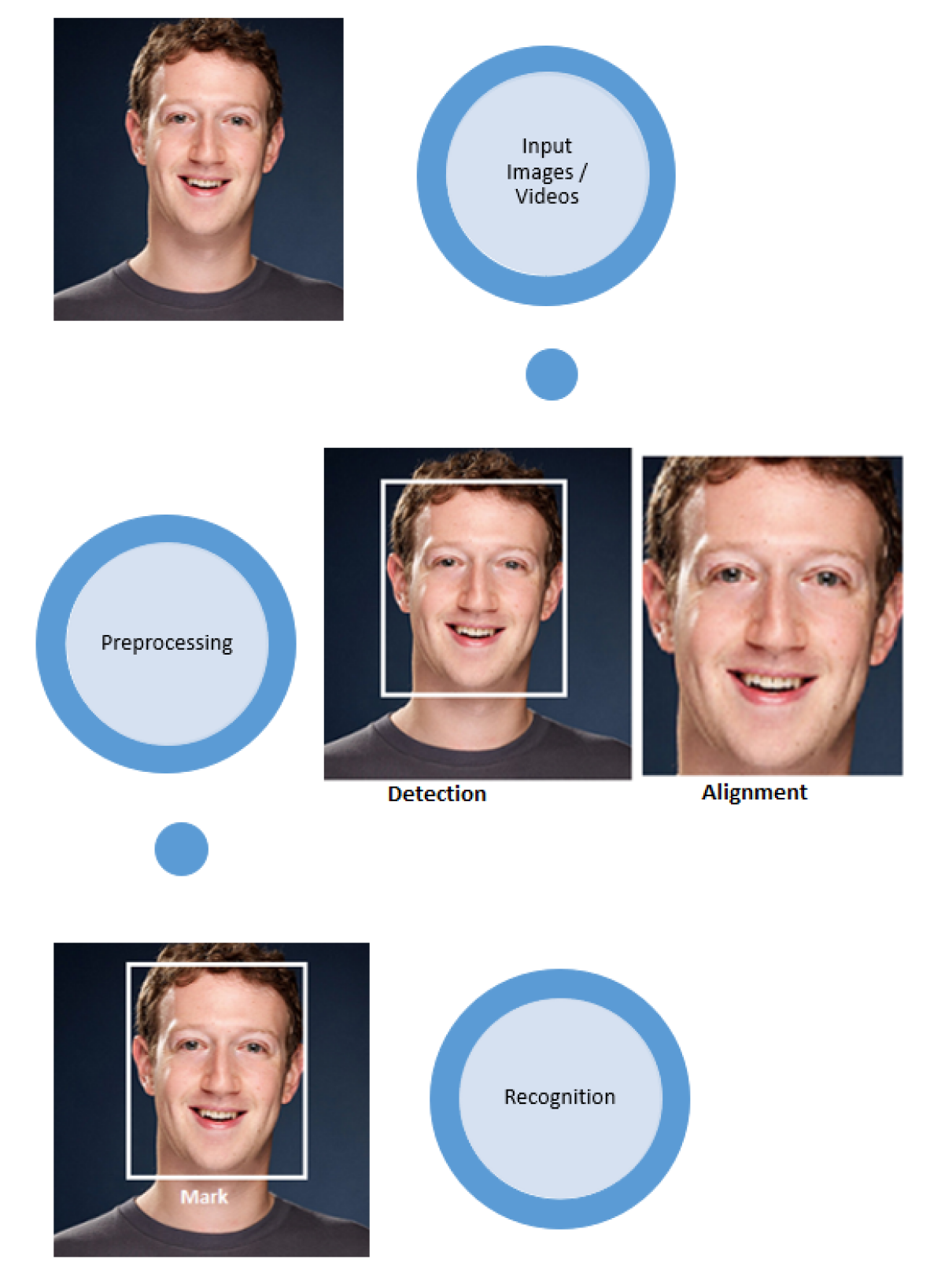
Figure 1: Face Recognition Pipeline.

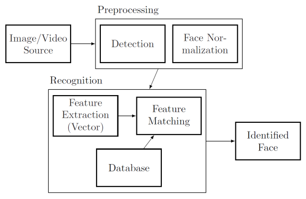
Figure 2: Face Recognition Block Diagram.

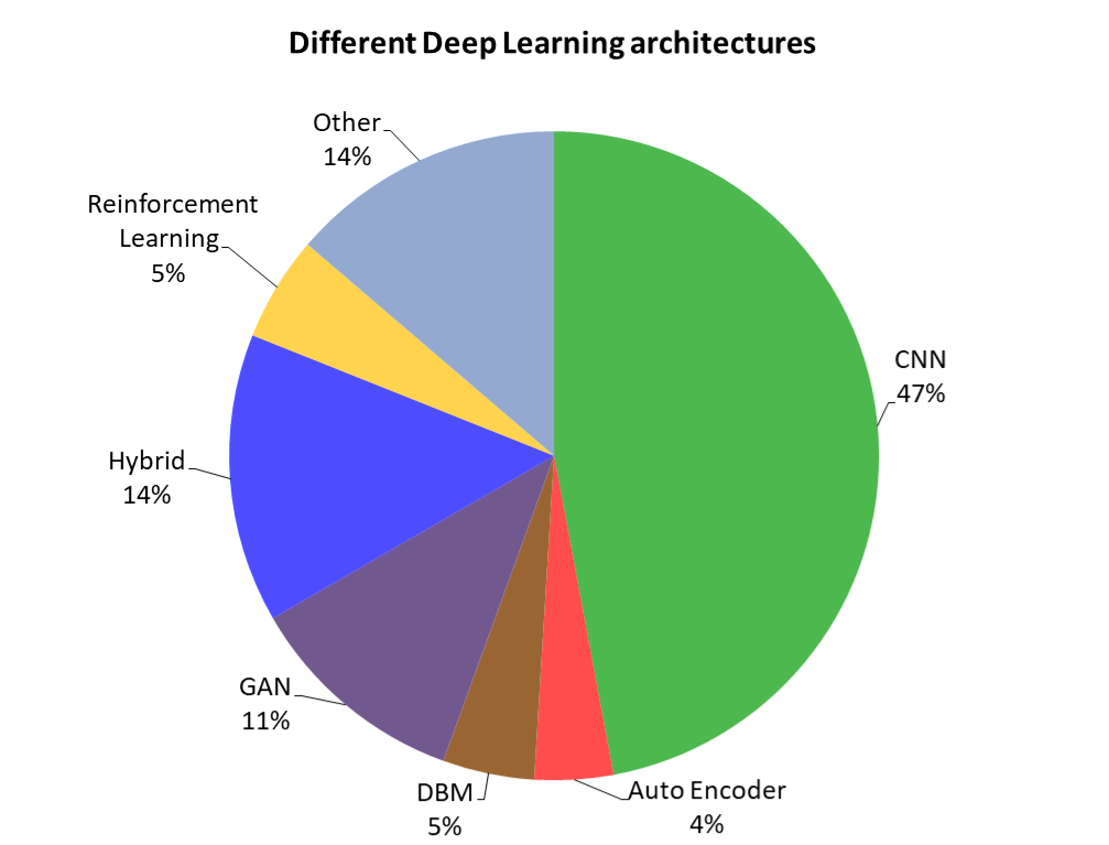
Figure 3: Different Deep Learning Architectures for Face Recognition.

Figure 4: Paper Distribution by Year.

I-A classical face detection

Face detection with a machine was started with some simple statistical techniques. Eigenfaces[1] was one of the most popular among them. It represents every image as a vector of weights obtained by projecting on eigenfaces components[2]. Researchers also tried to use some other traditional methods like elastic graph matching[3], Karhunen-Loeve based methods[4], singular value decomposition[5] for face recognition. Those methods were mostly tested on small datasets. Even in some cases, the size of the dataset was less than 100. Though statistical methods are not quite efficient, it gives the confidence that the machine itself can recognize the human face without external interference. It has a long-lasting certain impact on further improvement.

I-B feature extraction

The performance of any model on any particular dataset largely depends on the features extracted from the data. After using various methods on face detection, face alignment is also done using various statistical methods. Some face alignment methods are Active Appearance Model (AAM)[6], Active Shape Model (ASM)[7]. Those aligned faces are used for feature extraction. Some traditional methods for feature extraction are Local Binary Pattern[8], Fisher vectors[9]. Some dimensionality reduction methods like Principal Component Analysis (PCA)[10], Subclass Discriminant Analysis (SDA)[11] can be used for feature extraction. Depending on the priority area for feature extraction, it can be divided into local feature extraction and global feature extraction. Global feature generalizes the whole image; for example, Histogram of Gradient (HoG) and Bag of Words (BoW) use global feature extraction. On the other hand, local features extract the key points from the image, and one example of this method is Local Binary Patterns (LBP)[8]. Depending on how the features are extracted, feature extraction can be divided into many types; geometry-based technique, holistic approach, template-based technique, appearance-based approach, and color-based method are some of them. Also, several hybrid and hand-crafted[12] methods are traditionally used for face recognition. From time to time, feature extraction methods have been improved and robustly extracted more advanced features. So that face recognition methods can do their job more efficiently. Nowadays, Convolutional Neural Network (CNN) or Deep Convolutional Neural Network (DCNN) based methods are primarily used for feature extraction. Taking advantage of these feature extraction methods, we can implement face recognition efficiently using traditional machine learning methods like SVM[13].

I-C Artificial Neural Network

Artificial Neural Network (ANN), a network which is inspired by the biological neurons, got attention from various researchers. They tried to use it in face recognition in multiple forms. ANN was constructed for some specific purposes like data classification or pattern recognition. The main idea of using ANN for face recognition is to use extract features with different feature extraction methods and use them in different ANN combinations. WISARD (WIlkie, Stoneham and Aleksander’s Recognition Device)[14] was one of the initial models of ANN, which was used for face recognition[15]. It has a single-layer adaptive neural network structure. Taking advantage of Gabor features and LDA feature extraction models, ANN can recognize persons from images[16]. Fernandez et al.[17] started with detecting the face using Viola-Jones Algorithm and cropped it. Then they extracted the skin color, eyes color, the distance between the two eyes, the width of the nose, the height and width of the lips, and the distance between the nose and the lips from those cropped images. Those features are used in an ANN to identify a specific person.

I-D Deep Neural Network

Development of Deep Neural Network (DNN) and applying them into face recognition systems push recognition further ahead. DNN can extract more diverse features effectively from inputs which are never possible for ANN or other statistical methods. DNN is an extended version of ANN with multiple hidden layers in it. With some disadvantages, the more hidden layers in the DNN network, the more robust feature it can extract. Shepley[18] provided a critical analysis and comparison of different state-of-the-art DNN based face recognition methods in his survey paper and showed their benefits and problems. Learned-Miller et al.[19] discussed different approaches on the LFW dataset in their work. Balaban et al. [20] provided a brief introduction to the influences of the state-of-the-art deep learning methods in face recognition.

I-E Convolutional Neural Network

Due to the recent progress of Deep Convolutional Neural Networks (CNNs)[21], [22], the performance of state-of-the-art methods on image processing has significantly increased. Most of the CNN-based face recognition tasks are done by following the conventional pipeline of two steps. First is face detection and then recognition of those detected faces using different network architecture [23], [24], [25], [26]. However, there are some exceptions too [27]. CNN-based models mainly extract features from images and use them in face recognition. CNN can extract handy high-label features that are hard for a human to understand and different studies did the extraction in different ways. FaceNet[28] extract high-quality features from images and predict 128 elements from them and represent them in a vector named face embedding. This face embedding is used as the basis for training classifier systems. Some researchers [29], [25] also tried to recognize face from videos. Face tracking is the additional step to recognize a face from different frames of a video. In some controlled environments, CNN-based face recognition can do much better than humans.

I-F Deep Reinforcement learning

Reinforcement learning (RL) comes from the eagerness to mimic humans’ decision-making process. RL agents decide their behavior from environment experience using Markov Decision Process (MDP)[30]. Generally, RL is not used directly in face recognition. It is used as a part of a hybrid method like CNN and RL or GAN (Generative Adversarial Network) and RL. The researchers used RL to solve some problems, for instance, adaptation of loss functions[31], skewness embedding[32], user authentication [33], and searching a set of dominant features [34].

I-G loss function

Different deep learning-based face recognition models mainly differ in three main positions: dataset, network architecture, and loss function. A loss function is used to evaluate how well the model can predict the output by mapping with the actual output. If the model can predict the output properly, it produces a small value; otherwise, it provides a high value. Historically, with CNN, traditional softmax[35], [36] can be used for face recognition. However, some studies[37], [38] show that traditional softmax is not always quite sufficient for classification task. So, the researchers pay attention to develop more powerful loss functions. Most of the loss functions share the same idea of maximizing inter-class distance and/or minimizing intra-class distance [26] [38]. The preference of the loss function used in a model also depends on the neural networks activation function.

I-H Dataset

Finding a properly labeled and large dataset is another important criterion for developing a new and more accurate face recognition technique. Early dataset like CASIA-WebFace [39] to recent datasets like MS-Celeb-1M [40], VggFace2 [41] and IMDb [42] are playing their role to develop new techniques. With the improvement of multimedia technology, both datasets and the number of images are increasing. CASIA-WebFace [39] contains 0.5M images from 10,575 individuals. On the other hand, MSCeleb-1M [40] has about 10M images of 100K identities. As a result, there are some problems in the labeling of the data. The researchers like

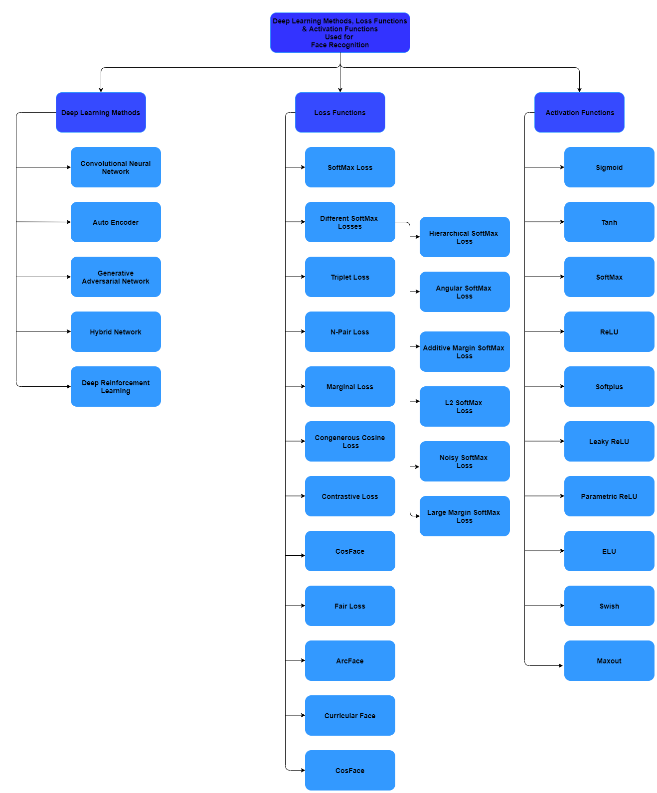
Figure 5: Taxonomy of the Deep Learning Methods, Loss Functions & Activation Functions used for Face Recognition.

Wang et al. [43], Wu et al. [44], and Deng et al.[45] tried to solve this problem. Depending on the labeled data, those face dataset can be divided into two types: open-set and close-set.

I-I 3D Face Recognition

3D face recognition can perform face recognition more efficiently than 2D face recognition. Because it does not face problems with light, pose, rotation, make-up, or blur images. Also, geometric information of 3D faces is more reliable than 2D faces. Initially, LDA, PCA, color-based methods, Gaussian, Gabor wavelet approach [46], [3] were mostly used for 3D face recognition. Most of the current methods are depending on DCNN, GAN, or pose variations. As 3D face data can not be used directly in face recognition, some pre-processing and feature extraction makes those data usable. 3D FR can be divided into two types depending on the extracted features: local feature-based methods[47] and global [48] feature-based methods. There is another technique called hybrid that is also used in feature extraction. It is a combination of local and global feature-based methods. It performs better than each technique individually. However, the main problem with 3D face recognition is, it does not have a large dataset. It is also not possible to collect data from websites like 2D faces. Also, it is a hard and time-consuming task to create dataset using infrared laser beams or 3D scanning. As a result, Bosphorus database[49] contains 4,652 scans of 105 individuals and CASIA-3D FaceV1 dataset [50] contains 4,624 scans of 123 individuals. Researches like [24], [51] provide ways to generate 3D dataset form 2D dataset.

I-J Paper summary

We have presented various types of deep learning architecture of face recognition system. In this paper, we have discussed different types of models, datasets, loss functions, and lots of occlusion handling techniques for FR task. A taxonomy of the deep learning methods, loss functions and activation functions used for Face Recognition is shown in Figure 5. Figure 4 shows the year-based distribution of the discussed papers and the most recent DL-based tasks for face recognition system have been discussed. Figure 3 shows the discussed DL methods of this paper. In the DL-based FR system, we have found that CNN plays an important role. Many types of FR tasks have been proposed based on the CNN model. Some of them are ResNet50, LightCNN-v9, SqueezeNetResNet-50, VGG16 and so on [52]. Other Deep Learning-based algorithms such as Autoencoder (AE), Generative Adversarial Networks, Deep Belief Networks, Hybrid Networks, and Deep Reinforcement Learning [53] have been briefly discussed in this paper. A Table has been constructed that merged the DL-based FR tasks with datasets, architectures, and accuracy.

Datasets are an essential factor in a machine learning system. DL algorithms can not do their job according to the user requirements without sufficient features in the datasets. LFW, YTF, YTC, IJB-A, IJB-B, IJB-C, CASIA-WebFace, MS-Celeb-1M, IMDb, VggFace2 and Celebrity-1000 datasets [52] are vastly used to train the DL-based FR system and test the performance of the model. We have also categorized some activation functions that are generally used in FR tasks. Most of these are Sigmoid, Tanh, Softmax, ReLu, Softplus, Leaky RelU, Parametric ReLU, ELU, Swish and Maxout [54]. Moreover, we have discussed Hierarchical Softmax Loss, Contrastive Loss, Triplet Loss, N-pair Loss, Marginal Loss, Ring Loss, COCO Loss and Softmax Loss [52]. Still image-based datasets and video-based datasets are also discussed. We have also took the most popular LFW dataset for comparing the accuracy of various models. In conclusion, recent Deep Learning-based face recognition methods have been thoroughly discussed in our paper.

I-K contributions

The highlighted points of this paper are noted below:

• Recent works on DL-based FR tasks have been discussed in our paper.

• Briefly introduce the new DL-based FR Models. e.g., Deep Belief Network, Deep Reinforcement Learning.

• Detail discussion of the loss functions and activation functions.

I-L organization

We have organized the rest of this paper in the following manner.

• II Deep Learning Methods: Face recognition models based on Deep Learning.

• III Comparison of Different Deep Networks: Comparison of Different Deep Networks by accuracy on a dataset.

• IV Loss functions and Activation functions: Different types of Loss functions and Activation functions are discussed in this section.

• V Challenges in Face Recognition Using Deep Learning: Occlusion and other various types of challenges has been discussed.

• VI Face Datasets: Most used still images and video datasets for Face Recognition tasks have been discussed in this section.

• VII Future Trends:Various types of application of DL-based FR tasks with the direction of Future Trends have been discussed here.

• VIII Conclusion: Overall summary of our work.

II Deep Learning Methods

II-A Convolutional Neural Network

Convolutional Neural Network [55] is the most popular Deep learning algorithm for image recognition, image classification, pattern recognition, and other feature extraction operation from an image[56]. There are many types of CNN algorithm. But basically, two types are presented here to explain the CNN algorithm. One is feature extractor and the other is the classifier. The name of CNN comes from a mathematical linear operation between two matrices known as convolution. In CNN, one matrix is the image and the other is the kernel (operator). Actually, an image is a simple single channel (gray-scale image) or three-channel (colour image) matrix, each entry in this matrix is one pixel of the image. The dimension of the image matrix is (HxWxD). Here, H=height, W=width and D=RGB channel for RGB colour image. The Grayscale image channel contains one and the colour image channel contains three RGB colour channel. The kernel (operator) is also a matrix that has dimension of (MxNxD). Here M and N are arbitrary but most popular kernels such as Edge detectors or other operators use 3x3 size kernel. Here, D means the depth or dimension of the kernel. The dimension of the kernel is similar to the image colour channel. Figure 6 describes the architecture of CNN. In Face Recognition systems, CNN shows an excellent performance and many models have been built from CNN architecture. Table I shows overview of CNN-based face recognition systems.

Figure 6: Basic CNN Architecture [57].

The basic CNN architecture contains four layers: the convolutional layer, pooling layer, non-linear, and fully-connected layer. The first two layers are parameterized, and the other two are non-parameterized [58]. Parameterized layers are convolutional layers and fully-connected layers. However, non-parameterized layers are nonlinear layers and pooling layers. However, this architecture may change according to the problem requirements. After modifying the CNN architecture, the researchers build many FR architectures, e.g. VGGNet, GoogLeNet, and ResNet, etc.[52] Most deep face recognition systems work in a supervised fashion[59].

Resnet50 is a CNN-based architecture that contains 50 layers and used for the supervised learning. A new dataset has been created manually named VGGFace2[41], which was used to train ResNet50 and SqueezeNet-ResNet-50[52] models. Wen and Li.[60] proposed a novel approach for age-invariant face recognition. The author claimed it as the first deep CNN-based age-invariant work. They used the largest dataset of age-invariant for training and tested and discussed the accuracy on various datasets.

TABLE I: Overview of CNN based Deep learning Models.

Algorithm	Dataset	Accuracy (%)	Description
ResNet50 [41]	IJB	0.995±0.001	A large-scale dataset named as VGGFace2 has been created and the authors compared its performance with CelebFaces+, LFW , and MegaFace datasets using the ResNet50 model.
SqueezeNet-ResNet-50 [41]	IJB	0.996±0.001	This model shows excellent performance on pose and age variation.
ResNet-64[26]	IJB-A	93.22	An elegant normalization approach for deep neural network called Ring loss.
ResNet-27[61]	LFW	99.48	The marginal loss simultaneously minimises the intra-class variances as well as maximises the inter-class distances by focusing on the marginal samples.
LightCNN-v29[62]	LFW	98.98	A low-resolution face recognition (LRFR) model which can perform nicely at the low resolution.
Deep CNN [63]	LFW	99.77	Deep Embedding Ensemble Model with 9 Convolution layers and a Softmax layer have been used to increase the performance.
MTCNN [37]	YTF	95	This model can be used in hyperspherical spaces when euclidean loss can be implemented into only euclidean spaces.
ReST[27]	LFW	93.4	An end-to-end face identification method inspired by a spatial transformer called ReST.
VGG16 [64]	300WLP	98	Feature learning-based face recognition model that used data synthesizing strategy to improve the accuracy on the diversity of pose.
NAN [29]	YouTube Face	95.72	Two attention blocks have been added with the CNN model.
DDRL[65]	YTF	94.2	Contains two parts a DCNN based encoding network and a distance metric module.
PDA[66]	VGGFace2-FP	95.32	Introduced multiple attention-based local branches at different scales to emphasize different discriminated facial regions.

Hu et al.[67] presented a CNN-based process, which improved face recognition performance. They added an extra layer with CNN, which was equivalent to Gated Two stream Neural Network (GTNN). Here, the authors proposed a robust nonlinear tensor-based fusion framework for face recognition, which can optimize Face Recognition Feature (FRF) and Face Attribute Feature (FAF) using low-rank tensor optimization and a GTNN. First, they systematically investigated and verified the various face recognition scenario, such as pose and illumination. Then, the authors applied a low-rank Tucker-decomposition of a tensor-based fusion framework, equivalent to GTNN, optimized by a neural network. The authors got 99.65% accuracy on the LFW dataset and 99.94% on CASIA NIR-VIS2.0 (Cross-modality environment). However, 100% accuracy was achieved using ±45º pose angle.

Face recognition accuracy has been improved using a pre-trained model of VGG-Face net and Lightened CNN[68]. A comprehensive analysis has been done based on some occlusion conditions. These conditions are upper and lower face occlusion, varying head pose angles, misalignment due to erroneous facial feature localization, and changing illumination of different strengths. Five popular datasets are used in this experiment. These datasets are AR face database, CMU PIE, Extended Yale dataset, Color FERET database and FRGC database. The authors[68] claimed that the FaceNet model achieved 95.12% accuracy on the YTF dataset and 99.63% accuracy on the LFW dataset. Again, applying the DeepFace Network increases the LFW datasets’ accuracy, which is 97.35% and the accuracy for the YTF dataset is 91.4%. DeepID network was trained on the Celebrity Faces dataset (CelebFaces) and tested on the LFW dataset, and achieved an accuracy of 97.45%. After modifying some architecture of the VGG-Face net and Lightened CNN model, the performance was also evaluated. Some factors such as illumination, occlusion, misalignment, and head pose had reduced the face recognition accuracy of the Deep learning model. In these cases, VGG-Face has achieved better performance than Lightened CNN. Five popular datasets, the AR face database, CMU PIE, Extended Yale dataset, Color FERET database, and the FRGC database, had been used in this experiment.

A new face identification-verification technique using a Deep Convolution Network was proposed, known as Deep IDentification-verification features (DeepID2)[69], by increasing inter-personal variations and reducing intra-personal variations of images. LDA, Bayesian face, and unified subspace models have limitations. These models are developed to handle inter and intra-personal variations. However, when the variations are more complex, these models show limited performance and achieved 99.15 ± 0.13% accuracy gain on the LFW dataset.

Chen et al.[62] proposed a low-resolution face recognition (LRFR) model. LRFR can perform creditably at the low resolution of the face smaller than 32*32 pixels. The authors gave priority to both angle discrepancy and magnitude discrepancy or magnitude gap between high resolution (HR) and corresponding low resolution (LR) face pairs. The purpose of the article was to recover the identity-aware information for LRFR. LR faces increase the angle and magnitude gap of the features. The authors claimed that all super resolution-based methods reduce the angled gap and magnitude gap among the features. That is why the super-resolution network achieved 98.46% accuracy on LightCNN-v9 and 98.98% on LightCNN-v29, which outperformed other renowned methods.

TABLE II: Overview of Auto-Encoder based Deep learning Models.

Algorithm	Dataset	Accuracy (%)	Description
U-net [70]	EURECOM	88.33	This mode deals with Illusion problem in thermal to visible cross-domain face matching.
DC-SSDA [71]	CMU-PIE	85	30% mouth occlusion and sunglass occlusion has been removed successfully from CMU-PIE face dataset.
$D^{2}$AE[72]	CelebA	87.82	Dispelling Autoencoder ($D^{2}$AE), a new framework that does not require previous knowledge to restore the occlusion part of the images.
CAN[73]	CACD-VS	92.3	Build the auto-encoder network that improve the face recognition performances by handling the Age variant problems.

To perform face verification and face re-identification task, Yu et al.[65] proposed a Deep Discriminative Representation Learning (DDRL) network. It has two parts a DCNN based encoding network and a distance metric module. Here, they used $l2$ distance to verify the two images were the same or not. On the other hand, they used softmax for face identification. Pointing out some problems with two folds face recognition, Wu et al.[27] proposed an end-to-end face identification method. Gathering inspiration from the spatial transformer, they proposed a module called Recursive Spatial Transformer (ReST). Their model has three parts: convolution layers, localization network, and spatial transformation layer. A DCNN (modified AlexNet) network with a softmax layer follows ReST and identifies the faces from the images. They also mentioned three different types of HiReST depending on the number of hierarchies (0-2).

On the other hand, Wang et al.[66] used an advanced CNN network for face recognition. They used a pyramid diverse attention to introduce multiple attention-based local branches at different scales to emphasize different discriminated facial regions at various scales automatically and adaptively. They presented a hierarchical bilinear pooling to combine features from different hierarchical layers. Lai et al.[23] used the idea to detect pores from face images for face recognition called PoreNet. At first, They extracted the pore features from high regulation face image using a scale-normalized Laplacian of Gaussian (LoG) blob detector. Then they matched those features with other images to classify them. They used Grid-based Motion Statistics (GMS)[74] to reject outline. PoreNet is modified version of HardNet[75]. A novel approach was proposed by Wen et al. [60] for Age Invariant Face Recognition (AIFR). This approach is a robust age-invariant deep face recognition framework. It is the first deep CNN-based age-invariant work, as they claimed. The coupled learning of latent factor-guided CNN (LIA-CNN) is beneficial to AIFR. It minimizes the classification error and maximizes the likelihood probability that latent factors generate from the training samples.

Yang et al.[29] presented a method for face identification and verification with a variable number of inputs face from image or video called Neural Aggregation Network (NAN). They extracted features from the image using CNN (GoogLeNet) network. Those features were passed through two attention blocks and assigned linear weights for them. For face verification, they used Siamese neural aggregation network and minimized average contrastive loss. Moreover, for face identification, they used a fully-connected layer followed by a softmax and minimize average classification loss. On the other hand, Kim et al.[25] mainly developed a method for face recognition from the video. This method also considers the upper body along with the face. In that paper, face detection was done by the same method as mentioned in[76] with some improvement in the network. Then they associated the body pose detected by OpenPose[77] with face information. Finally, these two data are used for face recognition with ResFace101[21]. Besides mentioning a method for augmenting the 3D face dataset, Gilani et al.[24] proposed a method to recognize them called FR3DNet. Their method maintains the same CNN-based architecture as [69] with some changes in convolution layers.

II-B Auto Encoder

Reconstructing an image from a noisy image is one of the great challenges for face recognition systems. Noisy images decrease the performance of a recognition system. Auto-Encoder is an excellent way to reconstruct a image. Table II shows the summary of auto-encoder techniques and performance. Auto-encoder is an unsupervised feature learning-based deep neural network which encodes and decodes the data efficiently[78]. It can automatically learn robust features from the large size of unlabeled data[79] and for this reason, the researchers use the autoencoder to encode the input into dimension reduction and represent it with significance. This technique has two stages: one is encoding, and the other is decoding. The entire architecture contained one or more hidden layers with an input and an output layer. In the encoding stage, the input compresses into a lower-dimensional feature with a meaningful representation. This process is continued until the required dimension is achieved. The next stage is the decoding phase. In this phase, the process is reversed to generate essential features from the encoded stage. The back-propagation is applied at the time of training models. The setting is set in the layer-by-layer decoding stage according to the input target size; thus, the error can be minimized. It decodes again, reconstructing the output similar to the original input. There are many variations in autoencoder techniques, for example, the denoising autoencoder[80] technique was proposed to improve the image representation ability of the autoencoder. A basic architecture is shown in Figure 7.

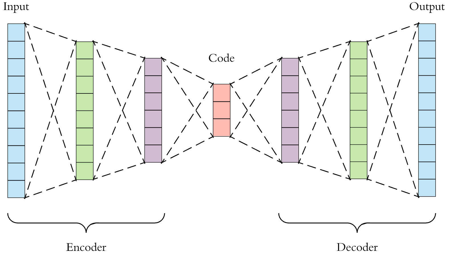
Figure 7: Basic Auto Encoder Architecture [81].

Though autoencoder combines the generative and learning properties to learn in an unsupervised manner, sometimes it can learn disentangled representations. Adversarial Latent Autoencoder (ALAE) [82] was proposed to handle this type of limitation. ALAE architecture improves the training procedure of GAN. Manifold-value data comes from the medical image. Higher-dimensional data arise when Magnetic Resonance Imaging (MRI) on brain connectomes in cognitive neuroscience. This higher dimensional space cannot reduce using PCA and for this reason, uncertainty arises when analyzing manifold-value. To overcome this situation Miolane et al.[83] proposed a Riemannian variational autoencoder but in low light condition, face recognition models can not perform properly. To solve the problem, Face matching in cross-domain thermal to visible techniques have been proposed. A deep autoencoder[70] based method learns from mapping between thermal and visible face images. Extensive works have been done using the Deep autoencoders and facial expression that can recognize images by reducing the dimensions[84].

The age-invariant problem in face recognition systems was solved by a couple of autoencoder-based face recognition techniques (CAN)[73]. CAN is constructed from two autoencoders and performed well for aging and de-aging on the complex nonlinear process using two shallow neural networks.

TABLE III: Overview of GAN based Deep learning Models.

Algorithm	Dataset	Accuracy (%)	Description
R3AN[85]	MegaFace	98.46	For cross model FR problems and experimented on public datasets.
ACSFC[86]	CASIA NIR-VIS 2.0	99.8±0.09	Improved the performance of NIR-VIS heterogeneous samples.
AFRN-GAN[87]	MULTIPIE	95.7	Combination of transfer learning and adversarial learning, proposed for cross-age FR.
Age-cGAN[88]	IMDB-Wiki cleaned	82.9	Improved the face aging system but can’t improve the face verification problem.
Age-cGAN+LMA[89]	LFW	88.7	Solve the drawbacks of Age-cGAN, and perform better in face verification.
DA-GAN[90]	IJB-A	99.1 ± 00.3	A face synthesis based model for extreme poses. Projects 3D face image to 2D using the learned knowledge from GAN.
TR-GAN[91]	Tufts Face	88.65	A cross model over thermal to RGB. GAN is used mainly for training the loss function.
DR-GAN[92]	CFP	93.41 ± 1.17	Solved the large pose variation. Performed well on both single and multi-image.
CpGAN[93]	CASIA NIR-VIS 2.0	96.63	For heterogeneous FR and Used perceptual loss in the model.
FI-GAN[94]	LFW	99.6	Improved the performance on large face pose based images.
PA-GAN[95]	IJB-A	99.0 ± 0.2	Increase the accuracy on raw surveillance of FR. Discriminativeness of a face is enhanced.

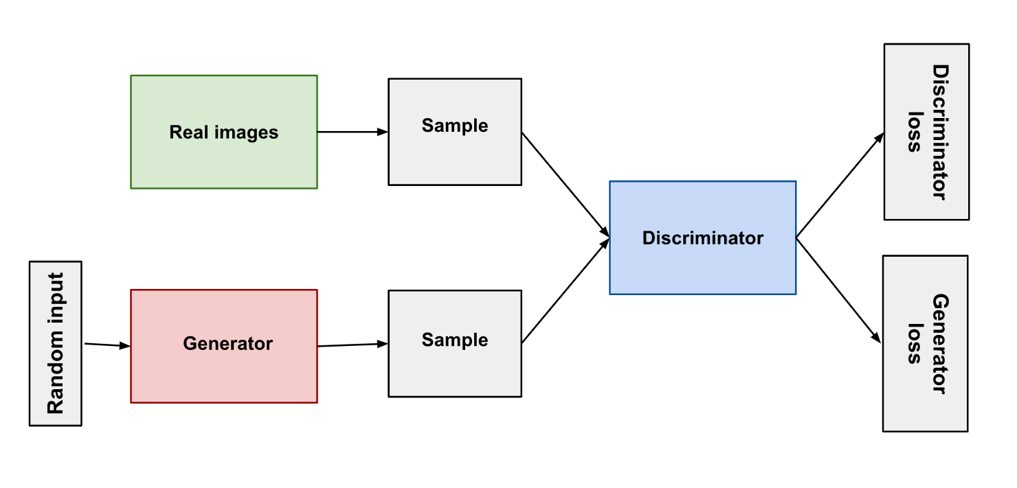
Figure 8: Basic GAN Diagram [96].

II-C Generative Adversarial Network

Generative Adversarial Networks are another kind of unsupervised deep learning method. It automatically discovers and learns the regularities or patterns from the input data. Figure 8 shows the block diagram of a GAN. The GAN model includes two sub-models: a generator model for generating new features and a discriminator model for classifying whether generated features are actual, taken from the domain, or fake, generated by the generator model. GANs are based on a game-theoretical schema where the generator network has to contend against an adversary. The generator part generates features and examples directly from its adversary, and the discriminator part tries to differentiate among the samples taken from the training data and the samples taken from the generator[97]. Table III describes the overview of GAN methods.

GANs are utilized in solving general face recognition problems as cross-age face recognition, face synthesis, pose-invariant face recognition, video-based face recognition, makeup-invariant face recognition, and so on. For example, R3AN architecture[85] was proposed for cross model FR problem. It divides the method into three paths: reconstruction, representation, and regression for training. Moreover, using a mapping function, it maximizes the conditional probability. TR-GAN[91] was proposed as a cross model over thermal to RGB. Here, GAN is used for loss training, and the generator part synthesizes images with fine details. For improving the performance of NIR-VIS heterogeneous samples, ACSFC[86] was proposed. It prototypes a high-resolution heterogeneous[98] face synthesis with two components: a texture inpainting component and a pose correction component. A novel 3D pose correction loss, two adversarial losses, and a pixel loss are used for generating results. DA-GAN[90] was proposed to do face synthesis under extreme poses. It merges the knowledge from adversarial training and domain from perception losses and projects 3D face image into 2D face image space.

A novel framework AFRN-GAN[87] was proposed for cross-age face recognition. It combines transfer learning (TL) and adversarial learning (AL). The discriminator part is trained to discriminate the age information, and the generator part extracts features using TL and suppresses age information using AL. Age-cGAN[88] was proposed to improve the aging system. However, it fails to improve much in the face verification sector. For overcoming this, Age-cGAN+LMA[89] was proposed. This combination improves the drawbacks of Age-cGAN. An encoder-decoder structure-based Disentangled Representation learning-Generative Adversarial Network, DR-GAN[92], was proposed to solve the large pose variation. Here, generator takes a face image, a pose-code $c$, and a random noise vector $z$ as the inputs to generate a face of the same identity with the target pose that can fool the discriminator. It works on both single image and multi-image. CpGAN[93] was proposed for heterogeneous face recognition. This model has two sub-networks; each has a separate GAN. The first sub-network is for the visible spectrum, and the other one is for the non-visible spectrum. The authors used a dense encoder-decoder structure with multiple loss functions to keep the features from each sub-network close to each other. They also used perceptual loss function in the coupling loss function.

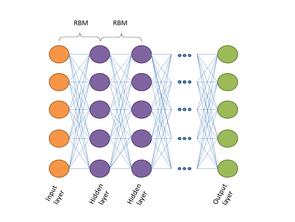
Figure 9: Deep Belief Network Architecture.

II-D Deep Belief Network

Traditional DNN-based networks have some problems such as stuck at local optima, slow learning and require a lot of training datasets. A type of DNN was proposed to cope with those problems, a composite of multiple hidden units called Deep Belief Network (DBN) [99]. In DBN, hidden units of different layers are internally connected, but the units of the same layers are not connected. It can be treated as a sequence of restricted Boltzmann machines (RBMs) or autoencoder where each hidden sub-layer works as a visible layer for the next hidden sub-layer. It generally ends with a softmax layer for classification. Figure 9 describes the Deep Belief Architecture. Table IV shows a brief overview of the deep belief network works on face recognition.

Taking advantage of convolutional restricted Boltzmann machines (CRBM), Huang et al.[100] developed a novel method to learn face recognition features. It is a local CRBM and applied to high-resolution images. They cropped the images into three different sizes and used them as inputs. Then, they divided the images into some overlapping regions and assigned a different set of weights for a different region. After that, they applied Information-Theoretic Metric Learning (ITML)[101] to produce a Mahalanobis matrix[102]. Finally, a linear SVM[13] was applied to perform face verification.

TABLE IV: Overview of Deep Belief Network based Models.

Algorithm	Dataset	Accuracy (%)	Description
Fan et al.[103]	ORL	93.5	Deep belief network with 2 hidden layers and 500 nodes each and 50% dropout.
Huang et al.[100]	LFW	87.77 ± 0.62	Novel local convolutional Restricted Boltzmann Machines, Information-Theoretic Metric Learning, Cholesky decomposition, SVM.
Annamalai and	ORL	98.92	Feature extraction using BRISK and LTP and
Prakash[104]	YALE	97.92	optimization with enhanced fire-fly.
Bouchra et al.[105]	BOSS	98.86	4 layers of neural network for DBN.
	MIT	98.04

Fan et al.[103] used DBN on a small Olivetti Research Laboratory (ORL)[106] dataset with two hidden layers with 500 units per layer for face recognition. As the dataset is small, the model might overfit. So, they randomly added 50% dropout to reduce that. As a result, their model achieved high accuracy, as they claimed. However, they did not mention how the dropout would react on a larger dataset.

On the other hand, Annamalai[104] divided the face recognition task into five sub-steps: image collection, image de-noising, feature extraction, optimization, and classification. The collected images are from ORL[106], YALE[107], and Face Semantic Segmentation (FASSEG)[108] databases. They used Histogram equalization for image de-noising, Local Ternary Pattern (LTP)[109] and Binary Robust Invariant Scalable Keypoints (BRISK)[110] for feature extraction and enhanced fire-fly[111] for optimization. Finally, a DBN network is used to classify the facial images. Bouchra et al.[105] made a comparison between three models on BOSS[105] and MIT[112] dataset. Those models are DBN with four layers, Stacked Auto-Encoder (SAE) with three layers, and Back Propagation Neural Networks (BPNN) with three layers. DBN outperformed the other two models on both datasets. DBM is sometimes used for liveness detection as an extended part of face recognition[113].

TABLE V: Overview of Hybrid Models based Face Recognition.

Algorithm	Dataset	Accuracy (%)	Description
CNN+RBM [114]	LFW	91.75	Deep ConvNets find the relation of a feature and Restricted Boltzmann Machine calculates the inference of feature extraction data.
DBMs + AEs [115]	WhoIsIt	28.53	Significantly increases the face recognition performance on weight and age variations.
MDLFace [116]	PaSC	93.4	Face recognition from Video datasets.
CAN [117]	FRGC Ver2.0	97.92	A cross modal based Deep learning method that can perform heterogeneous matching between depth and color of images.
DeepID3 [118]	LFW	99.52	VGG-net and GoogLenet Based hybrid model for Face Recognition.
CNN and deep metric learning [63]	LFW	99.77	This system performs on discriminative low dimensional features that improve the performance of face recognition.

II-E Hybrid Network

A hybrid model is a combination of two or more generic machine learning models to improve the overall performance of the model. In this technique, one algorithm augments another algorithm to solve problems precisely. Most of the time, a single machine learning algorithm is designed for a particular task. However, when two or more algorithms are combined, the performance of the hybrid model significantly increases. Some hybrid models are CNN+GAN, CNN+AE, GAN+RL, etc. Table V shows the summary of a Deep learning-based hybrid models for the face recognition system.

Sun et al.[114] proposed a combining ConvNet Restricted Boltzmann Machine for face verification. Generally, when the dataset comes with a high dimension and more complex feature vector, the dataset is needed to be compressed for feature extraction. Hybrid models are more robust process than a single algorithm for extracting features. CNN extracts features from two images; hence we can compare that both are similar or not. Here, the RBM method calculates the inference of image features to overcome the complexity. Sing et al. combined DBMs and AEs for face recognition[115]. This model follows the regularize-based process that easily learns facial-invariant problems. This method improves accuracy significantly. Goswami et al.[116] proposed a hybrid model named MLDFace. It is a combination of DBM and a stack of Denoising Autoencoders for the video-based face recognition framework. Another face recognition hybrid model, Conditional Adversarial Networks [117], was proposed to combine DCNN and GAN for cross-modality learning.

Instead of using traditional handcrafted features such as LBP or HOG, Liu et al.[63] introduced a two-stage face recognition method. It shows high-performance in the real-world face recognition system. Multi-patch deep CNN and deep metric learning methods are combined to build this model. This method can recognize faces with variant poses, occlusions, and expressions correctly. However, the number of faces and identities, data size, and the number of patches in training data are crucial for achieving the final performance. After a certain number of patches, the error rate of test data increases due to overfitting issues. When the authors combined ten models and train the data with that combined model, it showed the best result.

TABLE VI: Overview of Deep RL based Models.

Algorithm	Dataset	Accuracy (%)	Description
Fair Loss[31]	LFW	99.57	Learns margin adaptive strategy to make the additive margin more reasonable and solves the class imbalance problem.
ADRL[119]	YTF	96.52 ± 0.54	For video FR and use MDP for finding the attention of videos.
RL-RBN[32]	RFW[120]	95.79	Reduce racial bias by using RL.
AFA[121]	AGFW-v2	83.67	Face aging technique to generate a future face in old age from a young face in a video frame.
Xiaofeng et al.[122]	IJB-A	0.976±0.01	Focuses on set-based face verification and uses actor-critic reinforcement learning to create a dependency-aware attention control network.

Yang et al.[29] proposed Neural Aggregation Network (NAN) for video database based face recognition. This hybrid network is made using GoogleNet and Siamese neural aggregation networks. The authors extracted features from the image using CNN (GoogleNet), which passed through two attention blocks. For face verification, they used Siamese neural aggregation network and minimized average contrastive loss. For face identification, they used a fully connected layer followed by a softmax and minimize average classification loss. A hybrid network was proposed combining VGG-net and GoogLenet, named DeepID3[118], that improved face verification and identification accuracy using very DNN architecture. DeepID3 network is rebuilt from VGG-net and GoogLenet to change their exterior architecture. DeepID3 network shows excellent performance on LFW faces in verification and identification. When training on large-scale data, the efficiency will be increased. When the face labels are accurate, the accuracy of DeepID3 is 99.52% on the LFW dataset and 96.0% on the LFW Rank-1 dataset. DeepID3 net1 and DeepID3 net2 reduce the error rate by 0.81% and 0.26% compared to DeepID2+ net.

II-F Deep Reinforcement Learning

Reinforcement Learning learns from the adjacent environment. It originated from humans’ decision-making procedure[30], enabling the agent to decide the behavior from its experiences by trial and error. Figure 10 describes the basic Reinforcement Learning state diagram. The combination of Deep Learning and Reinforcement Learning is used mainly in face recognition. Researchers use it in various sectors of Face Recognition. Table VI shows a brief overview of RL in the face recognition method.

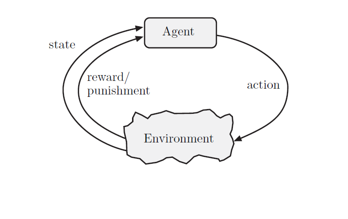
Figure 10: Basic RL Diagram [123].

In RL-RBN[32], the racial bias of face recognition has been reduced. The authors also proposed an optimal margin loss for this model. The authors had created two train datasets and applied the RL-based race-balance network. They also used the Markov decision process (MDP) to find the optimal margin for non-Caucasians. They worked on the self-created dataset. Chi et al.[121] used Deep RL for the face aging technique. It generates a future face of old age from a young face in a video frame. Here, the first step is to take feature embedding using CNN and normalize using VGG-19 with an additional extra conv3_1, conv4_1, conv5_1 layers. In this model, deep RL is used for neighbor selection. It can exploit the temporal relation among two consecutive frames. Here, each 900x700 resolution video frame needs 4.5 minutes.

In Fair Loss[31], the authors used Deep Q-Learning to train an agent to learn a margin-adaptive strategy to make the additive margin more reasonable for various classes. Moreover, it solves the class imbalance problem. In this model, first, they trained a CNN by manually changing the margin in the loss to collect a series of samples. Then, the samples were used to train an agent for the margin-adaptive strategy. Finally, they trained fair loss networks with margins changing by the action outputs from the agent. They used a two-layer fully connected network with proposed Q-function; a ReLU activation function follows each layer.

For video face recognition, an attention-aware deep reinforcement learning (ADRL)[119] was proposed. The authors made a system of finding videos’ attention as a Markov decision process and used deep RL for training the attention model. They took a pair of face videos as the input of the attention model. This framework has two parts: feature learning and attention learning. The first part is processed with a deep CNN model, a recurrent layer, and a temporal pooling layer, and the second part is a frame evaluation network, which produces the values of the frames. They introduced a flexible local bi-directional recurrent layer and a local temporal-pooling layer using long short-term memory (LSTM). They tried to adopt a human strategy using reinforcement learning to remove the worst frames step by step. The remaining frames are the most sensitive ones.

III Comparison of Different Deep Networks

We have set LFW dataset as the benchmark dataset and compared all the proposed methods’ accuracy in Table LABEL:tab:AllOverTable. In the Table, we place the FR methods from different years. In Figure 11, we have shown a gradually increasing graph of the performances. Though in 2016, the accuracy dropped by 0.1%.

TABLE VII: Verification Accuracy of the Deep Learning Methods on LFW Dataset.

Method	Category or	Training	Accuracy	Description
	Architecture	images	(%)
ConvNet-RBM[114]	Hybrid deep learning	240k	91.75	CNN for feature extraction and the RBM method calculates the inference of feature of two images.
HPEN[124]	3D Morphable Model		95.80	High -Fidelity Pose and Expression Normalization that automatically generates the face from frontal pose and expression.
Joint Bayesian[125]	Transfer learning	-	96.33	Invariance in feature-transform, low computational cost, robustness, subspace learning.
DeepFace[36]	Modified Deep CNN	2.6M	97.35	Training the model with a large-scale dataset of face images by a combination of automation and human with a small noise label.
Aug[126]	Data augmentation	2.4M	98.06	Increasing the amount of data by data augmentation and training them with deep CNN.
Cascaded Algorithm[127]	LightCNN	5M	98.19	Purifies noisy faces.
Multibatch[128]	Metric learning	2.6M	98.20	Reduced computational cost and increased precision.
FI-GAN[129]	GAN, Feature-Mapping Block	-	98.30	Face recognition and frontalization under large poses.
Multimodal[130]	Modified CNN	-	98.43	Extracts multimodal information from the holistic face, renders frontal pose, uniformly samples image using a set of CNN.
LF-CNN[131]	MTCNN	78k	98.50	Robust age-invariant deep face recognition framework, minimizes loss.
GaussianFace[132]	Gaussian Process	40k	98.52	Multi-task learning approach and self-acting adaption of complex data distribution form multiple source domains.
L-Softmax[133]	Modified loss function	-	98.71	Increased inter-class variation, adjusted margin and avoidance of overfitting.
VGGFace[69]	Modified CNN architecture	2.6M	98.95	A large-scale dataset with a minor small noise label was created and decreased annotation and fed them into a deep CNN.
DDRL[65]	Siamese network	-	99.07	DDRL consists of an encoding network and the distance metric module.
Baidu[63]	9 Convolution layers and a Softmax layer	1.3M	99.15	Deep CNN for multi patch feature extraction and metric learning for reducing the dimensionality.
DeepID2[134]	Multi-scale Deep Convolution network	202k	98.71	Increasing inter-personal variations and reducing intra-personal variations of image.
NormFace[135]	L2 normalization	-	99.15	Cosine similarity optimized by modifying Softmax loss and metric learning brings in agent vector of each class.
PSNet50[136]	Modified CNN	494k	99.26	Parametric Sigmoid-Norm (PSN) layer increases the gradient flow and performs better .
Center Loss[38]	Modified loss fuction	0.7M	99.28	Finds a vector called center for deep features of each class and decreases the distance between center and deep features during training.
SphereFace[37]	MTCNN, Advance Softmax loss	-	99.42	Used in hyperspherical spaces when the euclidean loss was implemented into only euclidean spaces.
DeepID2+[137]	Modified version of multiscale Deep CNN	290k	99.47	Dimensionality of the hidden layers of ConvNets increased and added supervision to early convolutional layers.
MarginalLoss[61]	Modified loss fuction, ResNet	4M	99.48	27 convolutional layers including batch normalization layers.
Face++[138]	Naive deep CNN	5M	99.50	Mainly focused on the importance of large labelled training dataset.
Range Loss [139]	Modified loss function	-	99.52	Finds the impact of imbalanced training dataset on deep learning model and handling methods.
DeepID3[118]	Modified CNN	290k	99.53	Architectural change in VGG net and GoogLeNet.
Fair Loss[31]	ResNet50, 64-layer CNN	-	99.57	Margin-aware reinforcement learning-based loss function.
DMHSL[140]	Improved triplet loss fuction	3.31M	99.60	A dynamic margin that decreases the number of triplets.
RegularFace[141]	Attention map created from low-rank bilinear pooling	3.1M	99.61	Finds the identical and relational pair features from attention score of local appearance block features of faces.
AdaptiveFace[142]	Modified Softmax loss function	5M	99.62	Adapted margin for various class variation and Hard Prototype Mining.
FaceNet[28]	CNN based ZF-Net and Inception architecture	-	99.63	Generates a high-quality face mapping from the images and provides a unified embedding through face image into a euclidean space.
GTNN[67]	Neural Tensor Fusion Networks	-	99.65	A robust nonlinear and low-rank Tucker-decomposition of tensor-based fusion framework.
CosFace[143]	Large margin cosine loss	-	99.73	A cosine margin term $m$ was introduced to maximize the decision margin in the angular space.
MobiFace[144]	Modified CNN architecture	3.8M	99.73	Deep neural network with lighter weight and low cost operator, low computational cost, high accuracy on mobile devices.
PRN[145]	ResNet-101	2.8M	99.76	Discriminate classes by unique pairwise relation and patches of local appearance in the region of landmark points into feature maps.
URFace[146]	Confidence-aware identification loss	4.8M	99.78	Handle different variation such as low resolution, occlusion and head pose by dividing the embedding into multiple sub-embeddings.
UniformFace[147]	Modified loss function	6.1M	99.80	Equidistributed representation in loss function to maximize discriminability between two classes.
HPDA[66]	Advanced CNN	-	99.80	Learns multiscale diverse local representation automatically and adaptively and also reduces problems like pose variations or large expressions, or similar local patches.
CurricularFace[148]	Adaptive Curriculum Learning	-	99.80	Connects positive and negative cosine similarity simultaneously without manual tuning and additional hyper-parameter.
FSENet[149]	Face Segmentor	8M	99.82	The local and global information of facial part utilized and structural correlation of them was built by face segmentor.
ArcFace[45]	ResNet100	-	99.83	A modified loss function, obtain highly discriminative features for FR and stabilize the training process.
AFRN[150]	Attention map created from low-rank bilinear pooling	3.1M	99.85	Finds the identical and relational pair features from the attention score of local appearance block features of faces.
GroupFace[151]	ResNet-100 and Group Decision Network	10M	99.85	Instance-based Representation and Group-aware Representation which provide self-distributed labels.
NAS[152]	Neural network search and modified loss function	5.8M	99.89	Combining reinforcement learning with neural network search.

However, this comparison is based on the data from the renowned models. After this, we take methods tested in the YTF dataset and present their accuracy in Table no VIII.

Figure 11: Accuracy distribution by year on LFW dataset.

TABLE VIII: Verification Accuracy of the Deep Learning Methods on YTF Dataset.

Method	Training Dataset	Accuracy (%)
DeepID[35]	CelebFaces	92.20
DeepFace[36]	-	92.50
DeepID2+[137]	CelebFaces+, WDRef	93.20
Range Loss[139]	VGGs	93.70
L-Softmax[133]	MNIST, CIFAR10, CIFAR100	94.00
NormFace[135]	-	94.72
CenterFace[38]	CASIA-WebFace, CACD2000, Celebrity+	94.90
TBE-CNN[153]	-	94.96
SphereFace[37]	CASIA-WebFace	95.00
FaceNet[28]	-	95.12
NAN[29]	-	95.72
MarginalLoss[61]	MS-Celeb-1M	95.98
DeepVisage[154]	MS-Celeb-1M	96.24
PRN[145]	VGGFace2	96.30
RegularFace[141]	CASIA-WebFace, VGGFace2	96.70
AFRN[150]	VGGFace2	97.10
VGGFace[69]	-	97.30
CosFace[143]	CASIA-WebFace	97.60
UniformFace[147]	MS-Celeb-1M, VGGFace2	97.70
GroupFace[151]	MSCeleb-1M	97.80
FSENet[149]	Ms-Celeb-1M, VGGFace2	97.89
ArcFace[45]	-	98.02
BiometricNet[155]	Casia, MS1M-DeepGlint	98.06

IV Loss Functions & Activation Functions

IV-A Different Loss Functions

The use of loss functions is an essential factor in machine learning-based methods. It helps the machine to learn and predict the results. If the expected result defers from the actual result in the training time, then loss functions try to minimize the difference and help to generate a better prediction. In Table IX, the classical loss functions and recent loss functions are described shortly.

IV-A1 Contrastive loss

Contrastive loss is a distance-based loss function used to compute the distance between the actual output and the predicted output. It provides the pairwise distance between two points through an equation. Contrastive loss can be shown like this:

$$D_{w}(X_{1},X_{2})=||G_{w}(X_{1})-G_{w}(X_{2})||$$ (1)

Here, we need to optimize the shared parameters w. $G_{w}(X_{1})$ and $G_{w}(X_{2})$ are the two points in the low-dimension space that generated by mapping images $x_{1}$ and $x_{2}$. If $x_{1}$ and $x_{1}$ belong to different class then contrastive loss function value will be large. Otherwise, the value will be small.

IV-A2 Triplet loss

Triplet loss[156] mainly focuses on both intra-class and inter-class difference. It creates a triplet which consists of baseline $x_{b}$, positive image $x_{p}$ and negative image $x_{n}$. Mathematically it is defined by:

$$TL(x_{b},x_{p},x_{n})=max(||x_{b}-x_{p}||^{2}-||x_{b}-x_{p}||^{2}+\alpha,0)$$ (2)

At first, three face images are needed to be provided where two of them are from the same person, and the third one is from a different person. This loss function’s objective is to minimize the distance from the baseline to the positive image ($x_{b}-x_{p}$) and maximize the distance from the baseline to the negative image ($x_{b}-x_{n}$). The negative image should be away from the positive image by a margin $\alpha$, just like SVM. It is mainly used for face verification tasks. Liu et al.[63] used this loss in their matrix learning step to reduce the features’ dimension. FaceNet[28] also used this loss in their work.

IV-A3 N-pair loss

N-pair loss[157] is more general version of triplet loss. It is applied on $N+1$ images. Among them $N-1$ are negative images and one positive image. The N-pair loss with $N+1$ example is defined by:

$$NP({x,x^{+},\{x_{i}\}_{i=1}^{(N-1)}};f)=log(1+\sum_{i=1}^{N-1}exp(f^{T}f_{i}-f^{T}f^{+}))$$ (3)

Here, $f$ is an embedding kernel. The deep neural network defines it. $x^{+}$ is the only positive example, and $x_{1},...,x_{N-1}$ are negative examples. When the number of negative examples is one, it works similarly to triplet loss.

IV-A4 Marginal loss

By minimizing the intra-class variances and maximizing the inter-class distances of the in-depth features, Deng et al. proposed a loss function to enhance discriminative power called marginal loss[61]. It mainly focuses on the marginal example and tries to minimize the difference between them. The function of marginal loss can be shown like this:

$$L_{m}=\frac{1}{m^{2}-m}\sum_{i,j,i\neq j}^{m}(\xi-y_{ij}(\theta-||\frac{x_{i}}{||x_{i}||}-\frac{x_{j}}{||x_{j}||}||_{2}^{2}))_{+}$$ (4)

Here, $x_{i}$ and $x_{j}$ are input images. $\theta$ is the threshold margin, and $\xi$ is the error margin for classification. $y_{ij}$ becomes -1 or 1 depending on whether $x_{i}$ and $x_{j}$ are in the same class or not. $(u)_{+}$ indicates that u is positive or zero. For marginal loss, $||x_{i}-x_{j}||$ is close to $\theta$ when $x_{i}$ and $x_{j}$ are from the same class otherwise is considerably away from $\theta$. Marginal loss can work individually or along with other traditional loss functions like Softmax.

IV-A5 Ring loss

Feature normalization through traditional normalization results in a non-convex formulation. To solve this, Zheng et al.[26] proposed an elegant normalization approach for the deep neural network called Ring loss. Mathematically it can be written as $L_{R}$ and shown in equation 5.

$$L_{R}=\frac{\lambda}{2m}\sum_{i=1}^{m}(F(x_{i})-R)$$ (5)

For image $x_{i}$, $F(x_{i})$ is the feature from deep neural network. Here, $m$ is the batch size, and $\lambda$ is the variable weight that has significant impact on the main loss function $L_{R}$. Moreover, the target norm value $R$ is also learned. In Ring Loss, Softmax, large-margin Softmax, or SphereFace is used as the primary loss function.

TABLE IX: Loss Functions.

Name	Function
Contrastive Loss	$D_{w}(X_{1},X_{2})=||G_{w}(X_{1})-G_{w}(X_{2})||$
Triplet Loss[156]	$TL(x_{b},x_{p},x_{n})=max(||x_{b}-x_{p}||^{2}-||x_{b}-x_{p}||^{2}+\alpha,0)$
N-pair Loss[157]	$NP({x,x^{+},\{x_{i}\}_{i=1}^{(N-1)}};f)=\log(1+\sum_{i=1}^{N-1}e^{(f^{T}f_{i}-f^{T}f^{+})})$
Marginal Loss[61]	$L_{m}=\frac{1}{m^{2}-m}\sum_{i,j,i\neq j}^{m}(\xi-y_{ij}(\theta-||\frac{x_{i}}{||x_{i}||}-\frac{x_{j}}{||x_{j}||}||_{2}^{2}))_{+}$
Ring Loss[26]	$L_{R}=\frac{\lambda}{2m}\sum_{i=1}^{m}(F(x_{i})-R)$
COCO Loss[158]	$L^{COCO}=\sum_{i\epsilon\beta}L^{(\,i)\,}=-\sum_{k,i}{t_{k}}^{(}i)\log p_{k}^{(\,i)\,}=-\sum_{i\epsilon\beta}\log p_{l_{i}}^{(\,i)\,}$
Softmax Loss	$f(\,s)\,_{i}=\frac{e^{s_{i}}}{\sum_{j}^{C}e^{s_{j}}};CE=-\sum_{i}^{C}{t_{i}}{\log(\,f(\,s_{i})\,)\,}$
L-Softmax Loss[133]	$L_{i}=-\log(\,\frac{e^{||W_{y_{i}}||||x_{i}||\psi(\,\theta_{y_{i}})\,}}{e^{||W_{y_{i}}||||x_{i}||\psi(\,\theta_{y_{i}})\,}+\sum_{j\neq y_{i}}e^{||W_{j}||||x_{i}||\cos{\theta_{j}}}})\,$
Hierarchical SoftMax Loss	$p(\omega=\omega_{0})=\prod_{j=1}^{L(\omega)-1}\sigma([[n(\omega,j+1)=ch(n(\omega,j))]].v^{\prime T}_{n(\omega,j)}h)$
	$where[[x]]=\big{\{}_{-1\quad otherwise}^{1\quad if\>x\>is\>true}$
A-Softmax Loss[37]	$L_{ang}=\frac{1}{N}-\log(\,\frac{e^{||x_{i}||\cos{m\theta_{y_{i},i}}}}{e^{||x_{i}||\cos{m\theta_{y_{i},i}}}+{}\sum_{j\neq y_{i}}e^{||x_{i}||\cos{\theta_{j,i}}}})\,$
AM-Softmax Loss[159]	$L_{AMS}=-\frac{1}{n}\sum_{i=1}^{n}\log{\frac{e^{s.(\cos{(\theta_{y_{i}})}-m)}}{e^{s.(\cos{(\theta_{y_{i}})}-m)}+\sum_{j=1,j\neq y_{i}}^{c}e^{s.\cos{\theta_{j}}}}}$
	$=-\frac{1}{n}\sum_{i=1}^{n}\log{\frac{e^{s.(W_{y_{i}}^{T}f_{i}-m)}}{e^{s.(W_{y_{i}}^{T}f_{i}-m)}+\sum_{j=1,j\neq y_{i}}^{c}e^{s.W_{j}^{T}f_{i}}}}$;
	where, $m=\cos{\theta_{W_{1}},P_{1}}+\cos{\theta_{W_{1}},P_{2}}$
L2-Softmax Loss[160]	minimize $-\frac{1}{M}\sum_{i=1}^{M}\log\frac{e^{W^{T}_{y_{i}}f(x_{i})+b_{y_{i}}}}{\sum_{j=1}^{C}e^{W^{T}_{j}f(x_{i})+b_{j}}}$
	subject to $||f(x_{i})||_{2}=\alpha,\forall i=1,2,...M.$
ArcFace[45]	$L_{3}=\frac{1}{N}\sum_{i=1}^{N}\log\frac{e^{s(\cos{(\theta_{y_{i}}+m)})}}{e^{s(\cos{(\theta_{y_{i}}+m)})}+\sum_{j=1,j\neq y_{i}}^{n}e^{s\cos{\theta_{j}}}}$
Noisy Softmax Loss[161]	$L=-\frac{1}{N}\sum_{i}\log\frac{e^{f_{y_{i}}-\alpha||W_{y_{i}}||||X_{i}||(1-\cos{\theta_{y_{i}}})|\varepsilon|}}{\sum_{j\neq y_{i}}e^{f_{j}}+e^{f_{y_{i}}-\alpha||W_{y_{i}}||||X_{i}||(1-\cos{\theta_{y_{i}}})|\varepsilon|}}$
CosFace[143]	$L_{l}mc=\frac{1}{N}\sum_{i}-\log\frac{e^{s(\cos{(\theta_{y_{i}},i)}-m)}}{e^{s(\cos{(\theta_{y_{i}},i)}-m)}+\sum_{j}\neq y_{i}e^{s\cos(\theta_{j},i)}},$
	subject to, $W=\frac{W*}{||W*||},x=\frac{x*}{||x*||},\cos(\theta_{j},i)=W_{j}^{T}x_{i}$
Fair Loss[31]	$L=-\frac{1}{N}\sum_{i=1}^{N}\log\frac{P*_{y_{i}}(m_{i}(t),x_{i})}{P*_{y_{i}}(m_{i}(t),x_{i})+\sum_{j=1,j\neq y_{i}}^{n}P_{j}(x_{i})}$;where $x_{i}\epsilon\mathbb{R}^{d}$
CurricularFace[148]	$L=-\log\frac{e^{s\cos({\theta_{y_{i}}+m})}}{e^{s\cos({\theta_{y_{i}}+m})}+\sum_{j=1,j\neq y_{i}}^{n}e^{sN(t^{(k)},\cos{\theta_{j}})}},$
	where, $N(t,\cos{\theta_{j}})=\{_{\cos{\theta_{j}}(t+\cos{\theta_{j}}),T(\cos\theta_{y_{i}})-\cos\theta_{j}\geq 0}^{\cos\theta_{j},T(\cos\theta_{y_{i}})-\cos\theta_{j}<0}$
	and $T(\cos\theta_{y_{i}})=\cos(\theta_{y_{i}}+m)$

IV-A6 Congenerous Cosine Loss (COCO Loss)

Yu et al.[158] proposed this loss by minimizing the cosine distance between samples. It reduces the complexity and normalizes the inputs. It also enlarges the distinction between inter-class and decreases the variation between inner-class.

IV-A7 Softmax Loss

Figure 12: Softmax Diagram.

The Softmax or Softargmax function is a generalization of logistic function to multiple dimensions [162]. It is commonly used in deep learning and neural networks. It is a combination of Softmax activation and cross-entropy loss that outputs the probability for every class, and later these will be summed up, shown in Figure 12.

IV-A8 Large-Margin Softmax Loss (L-Softmax)

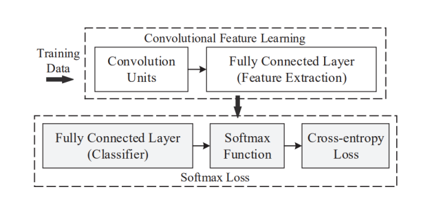
Figure 13: L-Softmax Diagram[133].

It is a modified softmax loss function that works with the distances between classes in CNN, proposed by Weiyang et al.[133]. It tries to maximize the distance between different classes and minimizes the distance between the same classes. As a result, intra-class compactness and inter-class separability boost the performance of recognition and detection tasks. It can also avoid overfitting. Figure 13 shows the workflow of L-Softmax.

IV-A9 Hierarchical Softmax

A faster and alternative loss function of Softmax is Hierarchical Softmax. The time complexity of Softmax is $O(n)$, where it can be done by Hierarchical Softmax in just $O(logn)$ time. In computation, it uses a multi-layer binary tree where each class is in the trees’ leaf node, and each edge contains a probability value. The probability is calculated with the product of values on each edge from the root to that node from that tree. The main advantage of hierarchical Softmax is that it works faster than the Softmax function. Wang et al.[163] used hierarchical Softmax with ABASNet in their multi-face recognition method.

IV-A10 Angular Softmax Loss (A-Softmax)

Weiyang et al.[37] proposed a model called SphereFace where they used a new loss that incorporates the angular margin. They changed the decision boundary of softmax loss to $||W_{1}||=||W_{2}||=1$ and $b_{1}=b_{2}=0$, which are weight and bias. So, the decision boundary becomes $||x||(cos(\theta_{1})-cos(\theta_{2}))=0$. Then, the decision boundary only depends on $\theta_{1}$ and $\theta_{2}$. It directly optimizes the angles, enabling CNNs to learn angularly distributed features. They used an integer $(m\geqslant 1)$ to quantitatively control the decision boundary and used it with $\theta_{1}$ and $\theta_{2}$ respectively in two classes, where $m$ controls the size of the angular margin.

IV-A11 Additive Margin Softmax Loss (AM-Softmax)

Wang et al.[159] proposed AM-Softmax for deep face verification. It is instinctively appealing and more efficient than the existing loss in margin-based work. It normalizes the weight and bias like A-Softmax. It uses an entirely new hyperparameter $s$, which measures the cosine value. The decision boundary is also adjusted according to the loss.

IV-A12 L2-Softmax Loss

For solving the performance gap of similarity score between positive pairs and negative pairs, Rajeev et al.[160] proposed a new loss L2-constrained Softmax Loss. It has an L2-constraint in feature descriptors which constricts the features to be on a fixed radius hypersphere by keeping the L2-norm constant. Forcing it to stay in a fixed radius minimizes the cosine similarity between the negative and positive pairs.

IV-A13 Additive Angular Margin Loss (ArcFace)

Jiankang et al.[45] proposed a new loss function called Additive Angular Margin Loss (ArcFace). It can obtain highly discriminative features for FR and stabilize the training process. Moreover, it also has a clear geometric interpretation due to its exact correspondence to geodesic distance on a hypersphere. The dot product between the DCNN feature and the last fully connected layer is equal to the cosine distance after feature and weight normalization. The arc-cosine function is used to determine the angle between the current feature and the target. The authors fixed the bias as zero, transformed the logit, fixed the individual weight by l2 normalization, fixed the embedding feature, and rescaled it.

IV-A14 Noisy Softmax Loss

Binghui et al.[161] tried to solve softmax loss’s early saturation behaviour by proposing noisy softmax loss. It migrates the early saturation problem by injecting annealed noise for every iteration and also brings continuous gradient propagation, which dramatically encourages the SGD solver.

IV-A15 CosFace: Large Margin Cosine Loss (LMCL)

Wang et al.[143] proposed a novel loss function, namely Large Margin Cosine Loss (LMCL). They applied L2 normalizing in both features and weight vectors and reformulated the softmax loss as a cosine loss. Then, a cosine margin term $m$ was introduced to maximize the decision margin in the angular space, dubbed Large Margin Cosine Loss (LMCL). The model, which is trained with LMCL, is named as CosFace. Authors contributed in 3 ways: (1) proposed a novel loss function called LMCL, (2) provided theoretical analysis for LMCL. (3) advanced the state-of-the-art performance over most of the famous face databases.

IV-A16 Fair Loss

For solving the imbalance problem, Bingyu et al.[31] proposed a new margin-aware reinforcement learning-based loss using Deep Q-Learning. They explored the adaptive boundaries between classes and proposed to balance the additive margins between various classes. They imitated all changes in additive margins for classes in the training process and collected influence on the training model. They concluded a strategy of adaptive margin by using Deep Q-learning.

IV-A17 CurricularFace: Adaptive Curriculum Learning Loss

Yuge et al.[148] proposed a credible method named CurricularFace using Adaptive Curricular Learning. CurricularFace solves convergence issues of features. It mainly addresses easy samples in preliminary stages and complex samples in later stages. Firstly, the curriculum construction is adaptive; the samples are randomly selected in each mini-batch. The curriculum is established adaptively via mining the hard online, which shows the diversity in samples with different importance. Secondly, the priority of complex samples is adaptive. The misclassified samples in mini-batch are chosen as complex samples and weighted by adjusting the modulation coefficients of cosine similarities between the sample and the non-ground class vectors.

IV-B Different Activation Functions

The activation function defines output depending on a given single input or a set of inputs in a node. It detects how much that node will contribute to the next node or nodes. The activation function can be both linear or non-linear. For deep learning, non-linear activation functions are highly preferable. Those can give a highly accurate output than the linear activation functions. There are many types of non-linear activation function. Table X shows a brief overview of commonly used activation functions.

TABLE X: Activation Functions.

Name	Function	Output Range
Sigmoid	$f(x)=\frac{1}{1+e^{-x}}$	(0, 1)
Tanh	$f(x)=\frac{e^{-x}-e^{x}}{e^{-x}+e^{x}}$	(-1, 1)
Softmax	$f(x)=\frac{e^{x_{i}}}{\sum_{i=0}^{N}e^{x_{i}}}$	(0, 1)
ReLU[164]	$f(x)=\big{\{}_{0\quad x\leq 0}^{x\quad x>0}$	$[0,\infty)$
Softplus[165]	$f(x)=ln(1+e^{x})$	$[0,\infty)$
Leaky RelU[166]	$f(x)=\big{\{}_{0.01x\quad x\leq 0}^{x\quad x>0}$	$(-\infty,\infty]$
Parametric ReLU[167]	$f(x)=\big{\{}_{ax\quad x\leq 0}^{x\quad x>0}$	$(-\infty,\infty]$
ELU[168]	$f(x)=\big{\{}_{a(e^{x}-1)\quad x\leq 0}^{x\quad x>0}$	-
Swish[169]	$f(x)=\frac{x}{1+e^{-\beta x}}$	-
Maxout[170]	$max(w_{1}^{T}x+b_{1},w_{2}^{(}T)x+b_{2})$	$[-\infty,\infty]$

IV-B1 Sigmoid

Sigmoid is one of the most popular probability functions. There are many types of sigmoid activation functions; one of them is the logistic activation function. It takes all possible values as input and provides output in the range of 0-1. Its output is an ”S”-shaped curve, also called a sigmoid curve. It is mainly used in the last layer to predict the output. It can show the probability of a new data point of being that class. The main problem with sigmoid is that it can not handle the vanishing gradient problem. It can only predict two classes; it is not possible to classify in multi-class with sigmoid activation. Some other sigmoid activations are used in face recognition are Adjustable Generalized Sigmoid, Sigmoidal selector.

IV-B2 Tanh

Hyperbolic tangent Activation Function, also known as Tanh activation function, is another sigmoid type activation function. Its output graph is also ’S’-shaped curve ranging between -1 to 1. It is mainly used in feed-forward neural networks. Being zero means it can handle both positive and negative values easily. It works better than the sigmoid activation function in almost all situations. Like sigmoid, it also cannot handle the vanishing gradient problem and can not classify in multi-class.

IV-B3 Softmax

Softmax is another popular activation function for DCNN, DNN, machine learning models. It is primarily used in the last layer for multi-class classification. It converts the output as a vector of probabilities of that data is in each class. The sum of the possibilities is one. It can take positive, negative, or zero, all possible values. It provides one output for every possible class in a normalized form in the range of 0 to 1. It solves the main problem of sigmoid and tanh activation function. It can classify into multi-class. Almost all CNN or DCNN based face identification researches, including [27], [65] used softmax in their last layer.

IV-B4 ReLU

Rectified Linear activation function or ReLU[164] is one of the most popular and sometimes default activation functions for many DCNN based models. It is a piecewise linear activation function that takes all possible values as input and output only when the values are positive and sets all negative values as zero. Its output range is 0 to infinity. Solving the vanishing gradient problem is not possible for Sigmoid and Tanh activation function, but it can be solved with ReLU. ReLU is faster than most of the other activation functions. ReLU also faces some problems. Its centre is not at zero and has no maximum limit. It sometimes comes to a state where the neuron becomes inactive and stuck there, especially in the first few layers. Also, no backpropagation can take the neuron out of it. It is called the dying ReLU problem. All popular DCNN based models for face recognition models use ReLU in their internal convolution layers. A smoother version of ReLU is Softplus[165]. Some other methods, including [171] use softplus as an activation function for their face recognition methods.

IV-B5 Leaky ReLU

Leaky Rectified Linear Activation, also known as Leaky ReLU or L-ReLU[166], is also a piecewise activation function that works with the same idea as ReLU. The only difference between ReLU and Leaky ReLU is when the input value is negative. Instead of setting zero like ReLU when the value is negative, Leaky ReLU multiplies the value with a small number $a$ (generally .01). So the negative portion gets a value but very small. It is an attempt to solve the dying ReLU problem. However, linearity is the main problem of leaky ReLU. So it can not be used in complicated classification tasks. Also, it is hardly possible to find out the perfect multiplayer value $a$.

IV-B6 Parametric ReLU

Parametric Rectified Linear Activation or Parametric ReLU or P-ReLU[167] is another version of Leaky ReLU. However, unlike Leaky ReLU, P-ReLU takes the slope of the negative portion as parameter $a$. The neural network finds it through gradient descent. It solves the problem of a predefined multiplier from Leaky ReLU. Nevertheless, it creates a new problem; it can act differently in a different situation.

TABLE XI: Overview of Still Image-based Face Recognition.

Algorithm	Method	Dataset	Accuracy (%)
ReST[27]	CNN	LFW	99.03
		YTF	95.40
DR-GAN[92]	GAN	IJB-A	94.7
		CFP	97.84 ± 0.79
Xiao et al.[172]	GAN	CMU MultiPIE	99.2
Peng et al.[64]	DNN	CMU MultiPIE	90.5
		300WLP	98.0
HPDA[66]	CNN	LFW	99.80
		CACD -VS	99.55
PW-GAN[173]	GAN	LFW	98.38
LF-CNN[131]	DCNN	LFW	99.5
		CACD	98.5
Li et al.[174]	CNN	MORPH	93.6
		CACD-VS	91.1
OE-CNNs[175]	CNN	Morph Album 2	98.67
		CACD-VS	99.5
		LFW	99.47
Wang et al.[176]	DAL	MORPH Album 2	98.93
		CACD -VS	99.40
Choi et al.[177]	DCNN	CMU Multi-PIE	96.24
Li et al.[174]	BLAN	Ms-celeb-1m	99.8
		Dataset 2[178]	82.7
		FAM [179]	97.0
RGMS[180]	DNN	ORL	98.75
		YALE	98.67
		AR dataset	92.30
NNAODL[181]	DL	LFW	93.1
		AR database	99.0
		ExYaleB	99.7

IV-B7 Exponential Linear Unit (ELU)

Exponential Linear Unit was also known as ELU[168]. It is also a piecewise activation function. It provides the same value as input, when the value is positive. However, when the input value is negative, its output is $\exp{(x)}-1$ multiplied by a constant value. The constant value is generally 0.1 or 0.3. As a result, it does not suffer from vanishing and exploding gradients problem. As it does not stick at zero on a negative value, so does not suffer from dying neuron as ReLU. Moreover, the most significant advantage is that it provides higher accuracy, and training timing is faster than ReLU in the neural network. Another type of ELU that also used in face recognition is Parametric ELU.

IV-B8 Swish

Swish[169] also provides a ReLU like output, where the input value is highly negative. The difference is that it does not change certainly at zero. From zero, it bends towards a negative value depending on a variable and creates a smooth curve. For positive values, it provides a positive output. In the Deep Neural Network test, swish always performs better than ReLU with every batch size. It is used in face recognition in [182].

IV-B9 Maxout

Maxout[170] is a simple piecewise activation function that provides the maximum of the input. It is a generalization of ReLU and Leaky ReLU activation functions. It takes advantage of the ReLU unit but does not have drawbacks. The main problem with maxout is that it doubles the number of computations in each neuron. As a result, it is much slower than ReLU. FaceNet[28] model used maxout activation in their fully connected layer for face recognition.

V Challenges in Face Recognition Using Deep Learning

Many challenges can be seen when we use face recognition in real-life scenarios. Those challenges keep us from getting the perfect accuracy. Deep learning methods try to solve the drawbacks and significantly improve accuracy. In recent years researchers focused on solving the challenges. We can notice several challenges in still image-based face recognition (SIFR), video-based face recognition (VFR), heterogeneous face recognition (HFR), etc.

V-A Still image-based face recognition

We can see more than half of the published papers on face recognition are on solving the SIFR challenges in the past. The problems are solved using CNN, AE, GAN, RL, etc. The researchers focus on solving pose variations problems, cross-age, illumination changes, facial makeup and expression variations. Table XI shows the summary of still image based face recognition methods.

V-A1 Pose-invariant

Nowadays, CNN-based models of face recognition have two-step pipeline: face detection and face recognition. In the ReST[27] paper, the authors discussed the problems of this two-step pipeline. Sometimes the alignment step transforms all faces into the same, and this causes geometrical information loss. We can see diversity when it comes to different poses, illumination, etc. However, in the two-step pipeline system, we lose this, which is essential for differentiation objects. To solve this problem, they design a novel Recursive Spatial Transformer module for CNN. It optimizes face alignment and recognition jointly in one network in an end-to-end system. The recursive structure has three parts: Convolutional layers, Localization network and Spatial Transformation layer. Here, the whole face is divided into hierarchical layers of regions, and each region is equipped with a ReST. It tries to handle large face variations and non-rigid transformations.

In DR-GAN[92], the author used Generative Adversarial Network for pose variations. They used an encoder-decoder structure-based Disentangled Representation Learning. In [172] Xiao et al. proposed a Geometric Structure Preserving-based GAN for multi-pose face frontalization. Here the perception loss compels the generator part to adjust the face image with the same input image. In the discriminator part, the self-attention block is used to preserve the geometry structure of a face. Sufang et al. [173] worked with large pose and photo-realistic frontal view synthesis variations in a generic manner and proposed a Pose-Weighted Generative Adversarial Network (PW-GAN). To solve problems like not being photo-realistic and losing ID information, they frontalized the face image through the 3D face and gave more attention to large poses, and they refined the pose code in the loss function.

Xiangyu et al.[124] proposed a method HPEN to recover the frontal face pose variation, which can recover the canonical-view of images using a 3D morphable model that automatically generates the face from frontal pose and expression. They created a 3D landmark from a 2D image using 3DMM (morphable method). Then, they used the mesh technique for the invisible position, and the invisible region was filled with the Trend fitting and Detail fitting method. However, this method’s main drawback is that it performs poorly when it comes to occluded images, and there is no clearance for large databases or real-time feedback. Peng et al.[64] tried to reconstruct from pose-invariant based images in their DNN based FR model. They reconstruct the 3D shape from a near-frontal face to generate new face images. They generate a non-frontal view from the frontal image and search the identity of the large embedded feature of identity and pose-variance. They also developed a feature reconstruction metric to learn the identity.

Wang et al.[66] proposed a pyramid diverse attention (PDA) to learn multiscale diverse local representation automatically and adaptively. They claimed this model reduces problems like pose variations or large expressions or similar local patches. They developed the model HPDA by fusing HBP and PDA. In HPDA, it can describe diverse local patches at various scales adaptively and automatically from varying hierarchical layers. Here, it guides multiple local branches in each pyramid scale to focus on diverse regions instead of face mark landing and a hierarchical bilinear pooling is combined. It also uses different cross-layer bilinear modules to integrate both high and low levels. This model has four parts: stem CNN, local CNN, global CNN, and classification. They use HSNet-61 in the background mainly. They also fused SENet and HSNet model. They used their own proposed divergence loss in diverse learning to guide multiple local branches to learn diverse attention masks. The diverse learning encourages each local branch to learn different attention masks by increasing their distances. Ding et al. [183] briefly discussed pose-invariant face recognition in their survey paper. The authors quoted the problems of PIFR as well as discussed possible future directions of Face Recognition tasks.

V-A2 Age-invariant

Age is always an essential factor in Face Recognition. We know that with the change of age, face changes. So, recognizing faces becomes more complicated when the test sample is aged. The researchers tried to solve this problem by experimenting with many deep learning models. Following it, Yandong et al.[131] proposed a deep CNN based age invariant face recognition named LF-CNN for deep face features. They extracted the age-invariant deep features from convolutional features by a carefully designed fully connected layer, termed as (LF-FC) layer. They developed a latent variable model, called latent identity analysis (LIA), to separate the variations caused by the aging process from the identity-related components in convolutional features. This model has two components: convolutional unit for feature learning and latent factor fully connected layer for age-invariant deep feature learning. They also used PReLU and max-pooling for enhancing robustness.

Li et al.[174] proposed a novel distance metric optimization technique that integrates feature extraction and the application of distance metrics and interaction between them using DCNN. It learns feature representation with an end-to-end decision function. They collected images from different age instances. Then they enlarged the differences between the unmatched pairs by reducing variations among matched pairs simultaneously. They used the mini-batch SGD algorithm to update the parameters, the top fully connected layer of the distance matrix, and the image features from the bottom layer.

TABLE XII: Overview of Video Face Recognition.

Algorithm	Method	Dataset	Accuracy (%)
NAN [29]	DCNN	IJB-A	0.986 ± 0.003
		YTF	95.72 ± 0.64
		Celebrity-1000	90.44
FBA [25]	DNN	JANUS CS3	85.3
ADRL[119]	RL	YTF	96.52 ± 0.54
		YTC	97.82 ± 0.51
Wang et al[184]	DCNN	Chinese citizen	98.92±0.005 (imbalanced)
		face image dataset[28]	94.36 ± 0.01 (balanced)
Liu et al [185]	RL	IJB-A	97.3±1.1
		YTF	96.01±0.48
		Celebrity-1000	91.37

The intra-class discrepancy has always been a problem in face recognition, especially in age-invariant problems. Wang et al.[175] proposed a novel Orthogonal Embedding CNNs (OE-CNNs) which decomposed the deep face features into two orthogonal components. It represents age-related and identity-related features. They used A-Softmax loss because different identities are discriminated by different angles and decomposed in spherical coordinates with radial coordinate and angular coordinates. The decomposed features improve performance. In reducing discrepancy on AIFR, Wang et al.[176] also proposed a novel algorithm. They tried to remove age-related components from features mixed with identity and age information. They factorized a new mixed face feature into two non-correlated elements: identity-dependent and age-dependent. They proposed the Decorrelated Adversarial Learning (DAL) algorithm, and a Canonical Mapping Module (CMM) was introduced, which found the maximum correlation of the paired features. The model learns the decomposed attributes of age and identity. To ensure the correct information, it simultaneously supervised the identity-dependent attribute and the age-dependent attribute. The proposed model has an extension of CCA, the Batch Canonical Correlation Analysis (BCCA). This method significantly increases the state-of-the-art (SOTA) on AIFR datasets.

Besides age and pose-invariant challenges in still image-based face recognition, we can see many challenges, such as facial makeup, illumination changes, partial face, facial expression, etc. Recently many researchers have started work on these challenges. Choi et al.[177] used a DCNN model for eliminating illumination effects and maximizing discriminative power. Zhao et al.[186] used a modified local binary pattern histogram (LBPH) for solving illumination diversification, expression variation and attitude deflection. Du et al.[181] proposed a framework for illumination changes and occlusion in face recognition named Nuclear Norm based Adapted Occlusion Dictionary Learning (NNAODL). They used a two-dimensional structure and dictionary learning (DL) in their framework. Li et al.[187] proposed a bi-level adversarial network (BLAN) for makeup problems in FR. To overcome posture, illumination and expression problems, Mona et al.[180] proposed a novel approach called Relative Gradient Magnitude Strength (RGMS) for feature extraction. This method is based on Deep Neural Networks (DNNs).

V-B Video-based face recognition

Video-based FR (VFR) is difficult in comparison with still image-based face recognition. When it comes to VFR, various problems come forward. Most of the videos usually come from mobile, which causes large pose variations, occlusions, out-of-focus blur, motion blur, etc. On the other hand, surveillance cameras, CCTV cameras cause cross-domain problems, and low-quality problems, etc. Researchers tried to partially solve pose-variations and occlusion in SIFR using the embedding technique [137], [63], but in VFR, the techniques are not extended. Some methods which are mainly proposed for SIFR but also work quite well for VFR, for example, DeepFace[36], DeepID2[134], FaceNet[28], VGGFace[69], C-FAN[188] etc. In C-FAN, Sixue et al. trained the model using CNN for SIFR and learned the quality value-added to an aggregation module. It performs well in VFR as it aggregates deep feature vectors in a single vector for face in the video. Table XII shows the overview of video based face recognition methods.

Jiaolong et al.[29] proposed a Neural Aggregation Net-work (NAN) for VFR. As input, it takes a set of face images or face video and produces a compact, fixed-dimension feature representation. They used DCNN for feature embedding, and for face verification, Siamese neural aggregation network and minimized average contrastive loss is used. On the other hand, a fully connected layer followed by a softmax and classification loss is used for identification. Kim et al.[25] proposed a novel approach, face and body association (FBA) in VFR. They used a retrained YOLO detector in face detection and a single DNN with ResNet-50 as backbone architecture in verification. For a video frame, they extract 18 key points in the 2D joints of the skeleton person. The data association stage has a scoring function, greedy data association, tracklet initialization and termination, tracklet filtering, and parameter settings like sub-stages. However, it treats the face and upper body as similar. Recently, there are some works on VFR using deep reinforcement learning such as ADRL[119], automatic face ageing[121] etc. For the real-time video, Wang et al.[184], and Grundstrom et al.[189] proposed DCNN based models. Liu et al.[185] proposed a dependency aware attention control (DAC) model, which used a reinforcement learning-based sequential attention decision of image embedding.

TABLE XIII: Image Datasets for Face Recognition.

Name	Number of	Total Images	Description
	Individuals
AgeDB[190]	570	16,516	Manually collected images of age range from 1 to 101. All of
			those images are taken from a uncontrolled environment with
			different pose, lighting, and noise.
Large Age-Gap (LAG)[191]	1,010	3,828	A dataset with images of people with large age difference.
CAF[175]	4,668	313,986	It is a noise free dataset containing images collected from
			Google. It also contains some images of Asian individuals.
CAFR[192]	25k	1,446,500	All images are annotated with identity, gender, age, and race.
			The age range is from 1 to 99 and divided into 7 age phases.
CPLFW[193]	5,749	11,652	Pose difference and the number of images are more balanced
			than LFW.
Trillion-Pairs[194]	5.7k	274k	Mainly used for testing. It is divided into two parts: ELFW,
			DELFW.
IMDb-Face[42]	59K	1.7M	Clean dataset collected from movie screenshots and posters.
MS1M-DeepGlint[194]	86,876	3,923,399	Large scale aligned face for training.
Asian-DeepGlint[194]	93,979	2,830,146	Large scale aligned face for training.
GANFaces-500k[195]	10k	500k	Synthetic dataset mainly used for training.
GANFaces-5M[195]	10k	5,000k	Synthetic dataset mainly used for training.
LFW[196]	5,749	13,233	Images with variation in pose, ethnicity, lighting, age,
			expression, background, gender, clothing, hairstyles, camera,
			quality, color saturation, and other parameters.
CelebFaces[114]	5, 436	87, 628	Images of celebrities collected from web used for training.
CASIA-WebFace[39]	10,575	494,414	Contains images of celebrities who were born between
			1940 to 2014 and mainly used for training.
VGG Face[69]	2,622	2.6M	A large dataset of publicly available images for training.
VGG Face2[41]	9,131	3.31M	A large dataset for training with a large variations in pose,
			age, illumination, ethnicity and profession.
MegaFace[197]	690k	1M	Used as a image gallery.
MS-Celeb-1M[40]	100k	10M	Images of celebrities, mainly for training set.
RMFRD[198]	525	95k	Two types of images for same persons: wearing mask and
			without wearing mask.
SMFRD[198]	10k	500k	Use of a software to automatically create faces with mask on
			popular face datasets.
KomNET[199]	-	39.6k	Those images are collected from 3 different sources: phone
			camera, digital camera and social media without
			considering lighting, mustache, beard, background, haircut,
			expression, and head covered glasses.

V-C Heterogeneous face recognition

Besides VFR and SIFR, Heterogeneous Face Recognition remains a challenging problem as cross-modality has limited training samples as well as complicated generation procedure of face images. Cao et al.[200] proposed a GAN-based asymmetric joint learning (AJL) process, which transforms the cross-modality variance. Wu et al.[201] proposed a CNN-based coupled deep learning (CDL) method to seek a shared feature space. In this method, heterogeneous images are treated as homogeneous images. Di et al.[202] proposed a hybrid model using GAN and CNN, which focused on extracting images from the visible range for synthesizing and took thermal images as input. He et al.[203] also proposed CFC, a GAN-based model for solving heterogeneous face synthesis problems. Jos et al. [204] proposed to extend the DL breakthrough for VIS face recognition to the NIR spectrum without retraining the underlying deep models that see only VIS faces. It has two core integrants, cross-spectral hallucination, and low-rank embedding. Cross-spectral hallucination produces VIS faces from NIR images through a DL approach. Low-rank embedding restores a low-rank structure for the deep features of faces across both the NIR and VIS spectrum. Ouyang et al.[98] discussed briefly in their survey paper on heterogeneous FR. Here, they quoted NIR-based faces, sketch-based faces, 3D faces, low-resolution images, etc. They also discussed their observation on the paper and some future directions, for example, computing time, datasets, alignment, technical methodologies, training volume, etc.

TABLE XIV: List of Video Datasets for Face Recognition.

Name	Total Videos	Number of Individuals	Description
IARPA Janus Benchmark A (IJB-A)[29]	2,042	500	The videos contain pose variation.
IARPA Janus Benchmark-B (IJB-B)[205]	7,011	1,845	Here, approximately 4 videos/subjects are available and average of 30 frames for each subject. This dataset contains more geographical distribution.
IARPA Janus Benchmark-C (IJB-C)[206]	11,779	3,531	This dataset have been created after removing the celebrity divergence. More pose variations are also included.
YouTube Face (YTF)[29]	3,425	1,595	The lengths of videos vary from 48 to 6,070 frames. The average video length is 181.3 frames.
YouTube Celebrities (YTC)[207]	1,910	47	All the entity has been converted into MPEG4 format. The videos has 25fps rate.
Celebrity-1000[29]	159,726	1,000	The videos contain celebrity images with 15 frames per second.
FaceSurv[208]	460	252	Benchmark face detection and face recognition dataset with different spectra and resolutions.
UMDFaces[209]	22,075	3,107	3,735,476 video frames have annotated from 22,075 videos. This dataset also figured out pose (pitch, roll, yaw), twenty-one key-points location and generated the gender information.
PaSC [210]	2,802	265	The videos have been collected based on many types of variations, such as location (inside and outside of buildings), pose, distance (both near and far from camera) and one video camera control with five held video cameras.
VDMFP[211]	958	297	The dataset contains two types of videos: walking and conversation. The videos were collected to avoid various constraints such as illumination and pose.

TABLE XV: Heterogeneous Face Datasets for Face Recognition.

Name	Number of	Total Images	Description
	Individuals	or Videos
CUHK VISNIR[212]	2,800	5,600	Each person has two images one is optical another is near
			infrared photo.
NIR-PF [213]	276	5,300	Contains 16-20 NRI images of each subject with different
			view, lighting condition, distance and scale.
Polarimetric thermal [214]	60	-	Contains LWIR and VIS data from 3 different distances.
MGDB [215]	100	400	Four face sketch of each subject; 3 of them are drawn after
			3 different time duration from viewing the mugshot by the
			artist and 1 by hearing face description from the eyewitness.
e-PRIP [216]	123	123	Extends PRIP [217] database by adding sketch images for
			each subject.
UoM-SGFS [218]	300	600	Contains software generated sketches.
Extended UoM-SGFS [219]	600	1,200	Contains software generated colored sketches.
UHDB31 [220]	77	1,617	Captured images form 21 viewpoints for each subject.
LS3DFace[221]	1,853	31,860	Contains 3D images.
Lock3DFace [222]	509	5,711	Contains video clips of RGBD face with different occlusion
			pose, time lapse and facial expression.
RGB-D DB [223]	747	845k	With a few illumination change and continuous pose
			variations in RGB-D format.
NJU-ID [224]	256	13,056	Fifty one images per subject in different resolution.
ID-Selfie-A [225]	-	20,000	Ten thousand pair of selfies are taken from a stationary
			camera and ID photos from chips.
ID-Selfie-B [225]	547	10,844	Individual ID card images and variable number of selfies
			for each individual.

VI Face Datasets

VI-A Image Datasets

Face recognition is a complex task in the real world scenario. To do it perfectly large and correctly labelled training dataset is required. Collecting face images and label them properly is a time-consuming task. There are a lot of publicly available datasets those can be used for this purpose. Earlier datasets were small in size, less than hundred identities. As time passes, more researchers and companies have come into this field. They are investing their time and money, so the size of the datasets is getting large. Some of the publicly available datasets have already crossed a few million face images[42], [195]. Nowadays, most of the images to create a new dataset are collected from different social media or websites[199]. The main problem for face recognition from the images is that most of the features from the face change with the change of the pose or age. Pointing out this problem, some researchers added images of different pose and age limit[196], [193]. Some datasets also contain synthetic face images to increase the number of images in their collection, for instance, GANFaces500k[195]. After covid-19 breaks out, face recognition with face masks getting researchers’ attention. Some datasets of people with masks and without masks like RMFRD[198], SMFRD[198] are already publicly available. Table XIII shows some of the recent available datasets.

VI-B Video Datasets

Face recognition from video data is a great issue in this era. So the video-based FR machine learning algorithm has become more popular nowadays. Many videos data have been generated through YouTube, Facebook, Instagram, and other social media. However, for this process, more videos data need to be trained through machines, so that the model can achieve excellent performance. It is obvious that large-scale datasets are needed to show better accuracy for face recognition from video data. To improve the Video-based FR task, some excellent work has been done and the researchers collected video data that helped to enhance the accuracy of the system. It is also noted that five groups from world renowned institutions work on Point-and-Shoot Challenge (PaSC) video data to evaluate the accuracy of PittPatt algorithm[226]. Here, Table XIV shows different video face datasets (e.g. IJB-A, YTF, IJB-B, YTC, and IJB-C etc.) for face recognition and explains their properties.

VI-C Heterogeneous Face Datasets

Heterogeneous face recognition is a challenging but important. It is used in different types of applications like security and law enforcement. HFR is a problem of recognizing face from images of nontraditional sources of light such as Near Infrared (NRI), Sketch, or 3D images. Images of NRI datasets are taken under infrared instead of visible light. CUHK VIS-NIR [212], NIR-PF[213] contains image under infrared. Sketch images are human art of other human’s face. MGDB[215], e-PRIP[216] are recent sketch face image datasets for face recognition. On the other hand, LS3DFace [221] and Lock3DFace [222] databases contain 3D faces. Although HFR is getting popular and some datasets are available, most of the datasets are small in size. Table XV shows a brief overview of the recently available HFR datasets.

VII Future Trends

VII-A Dataset size and training time

DNN based face recognition has come a long way. Currently, the state-of-the-art networks can take millions of images to train and manage hundreds of millions of parameters to generate output. Some of those methods showed incredible results on testing datasets. But still, DNN has a long way to go. Most of the methods took a long time and large dataset to train. Researchers can search the way to develop methods which can be trained with small dataset and take short time. Bio-inspired methods can be a great help for them.

VII-B COVID-19

As the COVID-19 has broken out in recent years, some security measures have been taken to save the human species from this pandemic. Wearing masks is one of them, and for this reason, traditional face recognition methods are mostly useless in this unexpected situation. So, researchers should pay attention and search for new ways to detect faces or persons. Some researchers [198] have already started their work. But more should come and join them. The use of infrared cameras can be a good solution. Moreover, researchers can think of this type of scenario for FR.

VII-C Face Recognition in Infrared Faces

Whenever obstacles come between face and camera, regular face photos are not adequate for FR. To overcome this issue, the researchers can focus on Infrared (IR) face images nowadays. IR images provide a multi-dimensional imaging system. The multi-dimensional imaging system is used to get more accurate results in unfavorable conditions like object illumination, expression changes, facial disguises, and dark environments[227]. So, the researchers can improve algorithms which are focused on IR-based FR.

VII-D COST FUNCTION

In recent times, researchers have tried to improve the cost functions. They can try to merge existing loss functions like Softmax loss and Centre loss[228], [38]. They can also try to use various cost functions in different layers like yang et al.[229]. Mainly, the researchers need to find more efficient cost functions to decrease the computational time.

VIII Conclusion

Our paper has demonstrated the recent advances of Deep learning-based face recognition systems that are mainly focused on algorithms, architecture, loss functions, activation functions, datasets, and varied types of occlusion such as pose-invariant, illusion, expression of face, age, and variations of ethnicity etc. Most of the Face Recognition systems has been built using Deep learning and the architecture may be changed according to the dataset variations and performance improvement issues. Deep learning architecture has shown excellent performance in the face recognition systems in recent decades. Different types of datasets like still image-based, heterogeneous face image-based, video-based, and occlusion-based datasets are shown in our paper as summarized forms. Our paper found that LFR, IJB, YTF and Ms-celeb-1M have shown near perfect performance in various FR tasks. Occlusion based challenges still appear in the FR task. This situation hampers the performance of the FR systems. More datasets and novel algorithms may reduce the occlusion based problems. Despite some limitations and challenges of the face recognition tasks, these systems are improved significantly in recent years.

Md. Tahmid Hasan Fuad was born in Rajshahi, Bangladesh. He is currently pursuing a B.Sc. degree in Computer Science and Engineering (CSE) with the Khulna University of Engineering & Technology (KUET), Khulna, Bangladesh. His research interests include Image Processing, Computer Vision, Artificial Intelligence, Machine Learning, and Deep Learning. He has already worked on some exciting Android Development and Machine Learning based mini-projects. He has also done some mini-projects using C++, Python, Java etc.

Awal Ahmed Fime was born in Jashore, Bangladesh. He is currently pursuing the B.Sc. degree in Computer Science and Engineering (CSE) with the Khulna University of Engineering & Technology (KUET), Khulna, Bangladesh. His research interests include Computer vision, Artificial Intelligence, Signal processing, Machine learning, and Deep learning. He has already worked on some Web and Mobile Application using ASP.NET, CSS, JavaScript, Android throughout his study using latest technology.

Delowar Sikder was born in Patuakhali, Bangladesh. He is currently pursuing the B.Sc. degree in Computer Science and Engineering (CSE) with the Khulna University of Engineering & Technology (KUET), Khulna, Bangladesh. His research interests include Computer vision, Artificial Intelligence, Machine learning, and Deep learning. He has also keen interested to Automated system design, Web and Mobile Application Development. He has already worked on some interesting projects throughout his study using latest technology.

MD.AKIL RAIHAN IFTEE was born in Joypurhat, Bangladesh. He is currently pursuing a B.Sc. degree in Computer Science and Engineering (CSE) with the Khulna University of Engineering & Technology (KUET), Khulna, Bangladesh. His research interests include Deep Learning, Data Science, Artificial Intelligence, Machine Learning, and Natural Language Processing. He has already developed some projects using C, C++, Python, Java, HTML, SQL, etc. He is a regular participant in machine learning and data science competitions on an online platform such as Kaggle, Hacker-Earth, etc.

Jakaria Rabbi received a master’s degree in Computing Science from University of Alberta, Edmonton, Canada. He is currently working as an Assistant Professor at the department of Computer Science and Engineering (CSE), Khulna University of Engineering & Technology (KUET), Khulna, Bangladesh. His research interests include Machine Learning, Deep Learning, Computer Vision Artificial Intelligence, Data Science and Remote Sensing. He has authored and coauthored several articles in peer-reviewed Remote Sensing journal and IEEE conferences.

MABROOK S. AL-RAKHAMI (M’20–SM’16) received a master’s degree in information systems from King Saud University, Riyadh, Saudi Arabia, where he is currently pursuing a Ph.D. degree with the Information Systems Department, College of Computer and Information Sciences. He has worked as a lecturer and taught many courses, such as programming languages in computer and information science, King Saud University, Muzahimiyah Branch. He has authored several articles in peer-reviewed IEEE/ACM/Springer/Wiley journals and conferences. His research interests include edge intelligence, social networks, cloud computing, Internet of things, big data and health informatics.

ABDUL GUMAEI received the Ph.D. degree in computer science from King Saud University, in 2019. He worked as a Lecturer and taught many courses, such as programming languages at the Department of Computer Science, Taiz University, Yemen. He is currently an Assistant Professor with the College of Computer and Information Sciences, King Saud University, Riyadh, Saudi Arabia. He has authored and coauthored more than 30 journal and conference papers in well-reputed international journals. He received a patent from the United States Patent and Trademark Office (USPTO) in 2013. His research interests include software engineering, image processing, computer vision, machine learning, networks, and the Internet of Things (IoT).

OVISHAKE SEN was born in Thakurgaon, Bangladesh. Currently, he is pursuing a B.Sc. degree in computer science and engineering (CSE) with the Khulna University of Engineering & Technology (KUET), Khulna, Bangladesh. He has developed some exciting projects using C, C++, Python, Java, HTML, CSS, ASP.net, SQL, Android, and iOS. His research interests include natural language processing, computer vision, speech processing, machine learning, deep learning, competitive programming, and data science.

Mohtasim Fuad was born in Chattrogram, Bangladesh. He is currently pursuing a B.Sc. degree in computer science and engineering (CSE) with the Khulna University of Engineering & Technology (KUET), Khulna, Bangladesh. His research interests include computer vision, natural language processing, data science, machine learning and deep learning. He is currently working on deep learning projects.

MD. NAZRUL ISLAM was born in Chandpur, Bangladesh. He is currently pursuing a B.Sc. degree in computer science and engineering (CSE) with the Khulna University of Engineering & Technology (KUET), Khulna, Bangladesh. He has worked on some exciting projects and some collaborative works throughout his study. He has worked sincerely at one of the data science projects of OneBlood Blood Centers in a concerted effort with success. His research interests include machine learning, arm architecture, data science, deep learning, computer vision, RISC architecture, and natural language processing.

References

- [1] M. Turk and A. Pentland, “Eigenfaces for recognition,” Journal of cognitive neuroscience, vol. 3, no. 1, pp. 71–86, 1991.
- [2] R. Chellappa, C. L. Wilson, and S. Sirohey, “Human and machine recognition of faces: A survey,” Proceedings of the IEEE, vol. 83, no. 5, pp. 705–741, 1995.
- [3] L. Wiskott, N. Krüger, N. Kuiger, and C. Von Der Malsburg, “Face recognition by elastic bunch graph matching,” IEEE Transactions on pattern analysis and machine intelligence, vol. 19, no. 7, pp. 775–779, 1997.
- [4] M. Kirby and L. Sirovich, “Application of the karhunen-loeve procedure for the characterization of human faces,” IEEE Transactions on Pattern analysis and Machine intelligence, vol. 12, no. 1, pp. 103–108, 1990.
- [5] Y.-Q. Cheng, K. Liu, J.-Y. Yang, and H.-F. Wang, “A robust algebraic method for human face recognition,” in 11th IAPR International Conference on Pattern Recognition. Vol. II. Conference B: Pattern Recognition Methodology and Systems, vol. 1. IEEE Computer Society, 1992, pp. 221–222.
- [6] T. F. Cootes, G. J. Edwards, and C. J. Taylor, “Active appearance models,” in European conference on computer vision. Springer, 1998, pp. 484–498.
- [7] T. F. Cootes and C. J. Taylor, “Data driven refinement of active shape model search.” in BMVC, 1996, pp. 1–10.
- [8] T. Ojala, M. Pietikainen, and D. Harwood, “Performance evaluation of texture measures with classification based on kullback discrimination of distributions,” in Proceedings of 12th international conference on pattern recognition, vol. 1. IEEE, 1994, pp. 582–585.
- [9] F. Perronnin and C. Dance, “Fisher kernels on visual vocabularies for image categorization,” in 2007 IEEE conference on computer vision and pattern recognition. IEEE, 2007, pp. 1–8.
- [10] I. T. Jolliffe, “Principal components in regression analysis,” in Principal component analysis. Springer, 1986, pp. 129–155.
- [11] M. Zhu and A. M. Martinez, “Subclass discriminant analysis,” IEEE transactions on pattern analysis and machine intelligence, vol. 28, no. 8, pp. 1274–1286, 2006.
- [12] C. Ding, J. Choi, D. Tao, and L. S. Davis, “Multi-directional multi-level dual-cross patterns for robust face recognition,” IEEE transactions on pattern analysis and machine intelligence, vol. 38, no. 3, pp. 518–531, 2015.
- [13] C. Cortes and V. Vapnik, “Support-vector networks,” Machine learning, vol. 20, no. 3, pp. 273–297, 1995.
- [14] I. Aleksander, W. Thomas, and P. Bowden, “Wisard· a radical step forward in image recognition,” Sensor review, 1984.
- [15] A. Tolba, A. El-Baz, and A. El-Harby, “Face recognition: A literature review,” International Journal of Signal Processing, vol. 2, no. 2, pp. 88–103, 2006.
- [16] C. MageshKumar, R. Thiyagarajan, S. P. Natarajan, S. Arulselvi, and G. Sainarayanan, “Gabor features and lda based face recognition with ann classifier,” in 2011 International Conference on Emerging Trends in Electrical and Computer Technology, 2011, pp. 831–836.
- [17] M. C. D. Fernandez, K. J. E. Gob, A. R. M. Leonidas, R. J. J. Ravara, A. A. Bandala, and E. P. Dadios, “Simultaneous face detection and recognition using viola-jones algorithm and artificial neural networks for identity verification,” in 2014 IEEE REGION 10 SYMPOSIUM, 2014, pp. 672–676.
- [18] A. J. Shepley, “Deep learning for face recognition: a critical analysis,” arXiv preprint arXiv:1907.12739, 2019.
- [19] E. Learned-Miller, G. B. Huang, A. RoyChowdhury, H. Li, and G. Hua, “Labeled faces in the wild: A survey,” in Advances in face detection and facial image analysis. Springer, 2016, pp. 189–248.
- [20] S. Balaban, “Deep learning and face recognition: the state of the art,” in Biometric and Surveillance Technology for Human and Activity Identification XII, vol. 9457. International Society for Optics and Photonics, 2015, p. 94570B.
- [21] K. He, X. Zhang, S. Ren, and J. Sun, “Deep residual learning for image recognition,” in 2016 IEEE Conference on Computer Vision and Pattern Recognition (CVPR), 2016, pp. 770–778.
- [22] K. Simonyan and A. Zisserman, “Very deep convolutional networks for large-scale image recognition,” arXiv preprint arXiv:1409.1556, 2014.
- [23] S.-C. Lai, M. Kong, K.-M. Lam, and D. Li, “High-resolution face recognition via deep pore-feature matching,” in 2019 IEEE International Conference on Image Processing (ICIP). IEEE, 2019, pp. 3477–3481.
- [24] S. Zulqarnain Gilani and A. Mian, “Learning from millions of 3d scans for large-scale 3d face recognition,” in 2018 IEEE/CVF Conference on Computer Vision and Pattern Recognition, 2018, pp. 1896–1905.
- [25] K. Kim, Z. Yang, I. Masi, R. Nevatia, and G. Medioni, “Face and body association for video-based face recognition,” in 2018 IEEE Winter Conference on Applications of Computer Vision (WACV). IEEE, 2018, pp. 39–48.
- [26] Y. Zheng, D. K. Pal, and M. Savvides, “Ring loss: Convex feature normalization for face recognition,” in Proceedings of the IEEE conference on computer vision and pattern recognition, 2018, pp. 5089–5097.
- [27] W. Wu, M. Kan, X. Liu, Y. Yang, S. Shan, and X. Chen, “Recursive spatial transformer (rest) for alignment-free face recognition,” in Proceedings of the IEEE International Conference on Computer Vision, 2017, pp. 3772–3780.
- [28] F. Schroff, D. Kalenichenko, and J. Philbin, “Facenet: A unified embedding for face recognition and clustering,” in Proceedings of the IEEE conference on computer vision and pattern recognition, 2015, pp. 815–823.
- [29] J. Yang, P. Ren, D. Zhang, D. Chen, F. Wen, H. Li, and G. Hua, “Neural aggregation network for video face recognition,” in Proceedings of the IEEE conference on computer vision and pattern recognition, 2017, pp. 4362–4371.
- [30] M. L. Littman, “Reinforcement learning improves behaviour from evaluative feedback,” Nature, vol. 521, no. 7553, pp. 445–451, 2015.
- [31] B. Liu, W. Deng, Y. Zhong, M. Wang, J. Hu, X. Tao, and Y. Huang, “Fair loss: margin-aware reinforcement learning for deep face recognition,” in Proceedings of the IEEE international conference on computer vision, 2019, pp. 10 052–10 061.
- [32] M. Wang and W. Deng, “Mitigating bias in face recognition using skewness-aware reinforcement learning,” in Proceedings of the IEEE/CVF Conference on Computer Vision and Pattern Recognition, 2020, pp. 9322–9331.
- [33] P. Wang, W.-H. Lin, K.-M. Chao, and C.-C. Lo, “A face-recognition approach using deep reinforcement learning approach for user authentication,” in 2017 IEEE 14th International Conference on e-Business Engineering (ICEBE). IEEE, 2017, pp. 183–188.
- [34] M. T. Harandi, M. N. Ahmadabadi, and B. N. Araabi, “Face recognition using reinforcement learning,” in 2004 International Conference on Image Processing, 2004. ICIP’04., vol. 4. IEEE, 2004, pp. 2709–2712.
- [35] Y. Sun, X. Wang, and X. Tang, “Deep learning face representation from predicting 10,000 classes,” in Proceedings of the IEEE conference on computer vision and pattern recognition, 2014, pp. 1891–1898.
- [36] Y. Taigman, M. Yang, M. Ranzato, and L. Wolf, “Deepface: Closing the gap to human-level performance in face verification,” in Proceedings of the IEEE conference on computer vision and pattern recognition, 2014, pp. 1701–1708.
- [37] W. Liu, Y. Wen, Z. Yu, M. Li, B. Raj, and L. Song, “Sphereface: Deep hypersphere embedding for face recognition,” in Proceedings of the IEEE conference on computer vision and pattern recognition, 2017, pp. 212–220.
- [38] Y. Wen, K. Zhang, Z. Li, and Y. Qiao, “A discriminative feature learning approach for deep face recognition,” in European conference on computer vision. Springer, 2016, pp. 499–515.
- [39] D. Yi, Z. Lei, S. Liao, and S. Z. Li, “Learning face representation from scratch,” arXiv preprint arXiv:1411.7923, 2014.
- [40] Y. Guo, L. Zhang, Y. Hu, X. He, and J. Gao, “Ms-celeb-1m: A dataset and benchmark for large-scale face recognition,” in European conference on computer vision. Springer, 2016, pp. 87–102.
- [41] Q. Cao, L. Shen, W. Xie, O. M. Parkhi, and A. Zisserman, “Vggface2: A dataset for recognising faces across pose and age,” in 2018 13th IEEE International Conference on Automatic Face & Gesture Recognition (FG 2018). IEEE, 2018, pp. 67–74.
- [42] F. Wang, L. Chen, C. Li, S. Huang, Y. Chen, C. Qian, and C. Change Loy, “The devil of face recognition is in the noise,” in Proceedings of the European Conference on Computer Vision (ECCV), 2018, pp. 765–780.
- [43] X. Wang, S. Wang, J. Wang, H. Shi, and T. Mei, “Co-mining: Deep face recognition with noisy labels,” in Proceedings of the IEEE international conference on computer vision, 2019, pp. 9358–9367.
- [44] X. Wu, R. He, Z. Sun, and T. Tan, “A light cnn for deep face representation with noisy labels,” IEEE Transactions on Information Forensics and Security, vol. 13, no. 11, pp. 2884–2896, 2018.
- [45] J. Deng, J. Guo, N. Xue, and S. Zafeiriou, “Arcface: Additive angular margin loss for deep face recognition,” in Proceedings of the IEEE/CVF Conference on Computer Vision and Pattern Recognition, 2019, pp. 4690–4699.
- [46] A. Scheenstra, A. Ruifrok, and R. C. Veltkamp, “A survey of 3d face recognition methods,” in International Conference on Audio-and Video-based Biometric Person Authentication. Springer, 2005, pp. 891–899.
- [47] D. Huang, G. Zhang, M. Ardabilian, Y. Wang, and L. Chen, “3d face recognition using distinctiveness enhanced facial representations and local feature hybrid matching,” in 2010 Fourth IEEE International Conference on Biometrics: Theory, Applications and Systems (BTAS). IEEE, 2010, pp. 1–7.
- [48] J. Zhu, R. San-Segundo, and J. M. Pardo, “Feature extraction for robust physical activity recognition,” Human-centric Computing and Information Sciences, vol. 7, no. 1, p. 16, 2017.
- [49] A. Savran, N. Alyüz, H. Dibeklioğlu, O. Çeliktutan, B. Gökberk, B. Sankur, and L. Akarun, “Bosphorus database for 3d face analysis,” in European workshop on biometrics and identity management. Springer, 2008, pp. 47–56.
- [50] February 2021. [Online]. Available: http://biometrics.idealtest.org/
- [51] F. Liu, R. Zhu, D. Zeng, Q. Zhao, and X. Liu, “Disentangling features in 3d face shapes for joint face reconstruction and recognition,” in Proceedings of the IEEE conference on computer vision and pattern recognition, 2018, pp. 5216–5225.
- [52] G. Guo and N. Zhang, “A survey on deep learning based face recognition,” Computer vision and image understanding, vol. 189, p. 102805, 2019.
- [53] L. Liu, W. Ouyang, X. Wang, P. Fieguth, J. Chen, X. Liu, and M. Pietikäinen, “Deep learning for generic object detection: A survey,” International journal of computer vision, vol. 128, no. 2, pp. 261–318, 2020.
- [54] A. Apicella, F. Donnarumma, F. Isgrò, and R. Prevete, “A survey on modern trainable activation functions,” Neural Networks, 2021.
- [55] Y. Lecun, L. Bottou, Y. Bengio, and P. Haffner, “Gradient-based learning applied to document recognition,” Proceedings of the IEEE, vol. 86, no. 11, pp. 2278–2324, 1998.
- [56] M. Coskun, A. Ucar, O. Yildirim, and Y. Demir, “Face recognition based on convolutional neural network,” in 2017 International Conference on Modern Electrical and Energy Systems (MEES), 2017, pp. 376–379.
- [57] V. H. Phung, E. J. Rhee et al., “A high-accuracy model average ensemble of convolutional neural networks for classification of cloud image patches on small datasets,” Applied Sciences, vol. 9, no. 21, p. 4500, 2019.
- [58] S. Albawi, T. A. Mohammed, and S. Al-Zawi, “Understanding of a convolutional neural network,” in 2017 International Conference on Engineering and Technology (ICET), 2017, pp. 1–6.
- [59] D. Scherer, A. Müller, and S. Behnke, “Evaluation of pooling operations in convolutional architectures for object recognition,” in Artificial Neural Networks – ICANN 2010, K. Diamantaras, W. Duch, and L. S. Iliadis, Eds. Berlin, Heidelberg: Springer Berlin Heidelberg, 2010, pp. 92–101.
- [60] Y. Wen, Z. Li, and Y. Qiao, “Latent factor guided convolutional neural networks for age-invariant face recognition,” in Proceedings of the IEEE conference on computer vision and pattern recognition, 2016, pp. 4893–4901.
- [61] J. Deng, Y. Zhou, and S. Zafeiriou, “Marginal loss for deep face recognition,” in Proceedings of the IEEE Conference on Computer Vision and Pattern Recognition Workshops, 2017, pp. 60–68.
- [62] J. Chen, J. Chen, Z. Wang, C. Liang, and C.-W. Lin, “Identity-aware face super-resolution for low-resolution face recognition,” IEEE Signal Processing Letters, vol. 27, pp. 645–649, 2020.
- [63] J. Liu, Y. Deng, T. Bai, Z. Wei, and C. Huang, “Targeting ultimate accuracy: Face recognition via deep embedding,” arXiv preprint arXiv:1506.07310, 2015.
- [64] X. Peng, X. Yu, K. Sohn, D. N. Metaxas, and M. Chandraker, “Reconstruction-based disentanglement for pose-invariant face recognition,” in Proceedings of the IEEE international conference on computer vision, 2017, pp. 1623–1632.
- [65] J. Yu, D. Ko, H. Moon, and M. Jeon, “Deep discriminative representation learning for face verification and person re-identification on unconstrained condition,” in 2018 25th IEEE International Conference on Image Processing (ICIP). IEEE, 2018, pp. 1658–1662.
- [66] Q. Wang, T. Wu, H. Zheng, and G. Guo, “Hierarchical pyramid diverse attention networks for face recognition,” in Proceedings of the IEEE/CVF Conference on Computer Vision and Pattern Recognition, 2020, pp. 8326–8335.
- [67] G. Hu, Y. Hua, Y. Yuan, Z. Zhang, Z. Lu, S. S. Mukherjee, T. M. Hospedales, N. M. Robertson, and Y. Yang, “Attribute-enhanced face recognition with neural tensor fusion networks,” in Proceedings of the IEEE International Conference on Computer Vision, 2017, pp. 3744–3753.
- [68] M. Mehdipour Ghazi and H. Kemal Ekenel, “A comprehensive analysis of deep learning based representation for face recognition,” in Proceedings of the IEEE conference on computer vision and pattern recognition workshops, 2016, pp. 34–41.
- [69] O. M. Parkhi, A. Vedaldi, and A. Zisserman, “Deep face recognition,” 2015.
- [70] A. Kantarcı and H. K. Ekenel, “Thermal to visible face recognition using deep autoencoders,” in 2019 International Conference of the Biometrics Special Interest Group (BIOSIG). IEEE, 2019, pp. 1–5.
- [71] L. Cheng, J. Wang, Y. Gong, and Q. Hou, “Robust deep auto-encoder for occluded face recognition,” in Proceedings of the 23rd ACM international conference on Multimedia, 2015, pp. 1099–1102.
- [72] Y. Liu, F. Wei, J. Shao, L. Sheng, J. Yan, and X. Wang, “Exploring disentangled feature representation beyond face identification,” in 2018 IEEE/CVF Conference on Computer Vision and Pattern Recognition, 2018, pp. 2080–2089.
- [73] C. Xu, Q. Liu, and M. Ye, “Age invariant face recognition and retrieval by coupled auto-encoder networks,” Neurocomputing, vol. 222, pp. 62–71, 2017.
- [74] J. Bian, W.-Y. Lin, Y. Matsushita, S.-K. Yeung, T.-D. Nguyen, and M.-M. Cheng, “Gms: Grid-based motion statistics for fast, ultra-robust feature correspondence,” in Proceedings of the IEEE conference on computer vision and pattern recognition, 2017, pp. 4181–4190.
- [75] A. Mishchuk, D. Mishkin, F. Radenovic, and J. Matas, “Working hard to know your neighbor’s margins: Local descriptor learning loss,” arXiv preprint arXiv:1705.10872, 2017.
- [76] Z. Yang and R. Nevatia, “A multi-scale cascade fully convolutional network face detector,” in 2016 23rd International Conference on Pattern Recognition (ICPR). IEEE, 2016, pp. 633–638.
- [77] Z. Cao, T. Simon, S.-E. Wei, and Y. Sheikh, “Realtime multi-person 2d pose estimation using part affinity fields,” in Proceedings of the IEEE conference on computer vision and pattern recognition, 2017, pp. 7291–7299.
- [78] M. Z. Alom, T. M. Taha, C. Yakopcic, S. Westberg, P. Sidike, M. S. Nasrin, M. Hasan, B. C. Van Essen, A. A. Awwal, and V. K. Asari, “A state-of-the-art survey on deep learning theory and architectures,” Electronics, vol. 8, no. 3, p. 292, 2019.
- [79] F.-N. Yuan, L. Zhang, J.-T. Shi, X. Xia, and G. Li, “Theories and applications of auto-encoder neural networks: A literature survey,” Jisuanji Xuebao/Chinese Journal of Computers, vol. 42, pp. 203–230, 01 2019.
- [80] W. Wang, Y. Huang, Y. Wang, and L. Wang, “Generalized autoencoder: A neural network framework for dimensionality reduction,” in 2014 IEEE Conference on Computer Vision and Pattern Recognition Workshops, 2014, pp. 496–503.
- [81] “Comprehensive introduction to autoencoders,” https://towardsdatascience.com/generating-images-with-autoencoders-77fd3a8dd368. [Online]. Available: https://towardsdatascience.com/generating-images-with-autoencoders-77fd3a8dd368
- [82] S. Pidhorskyi, D. A. Adjeroh, and G. Doretto, “Adversarial latent autoencoders,” in Proceedings of the IEEE/CVF Conference on Computer Vision and Pattern Recognition (CVPR), June 2020.
- [83] N. Miolane and S. Holmes, “Learning weighted submanifolds with variational autoencoders and riemannian variational autoencoders,” in Proceedings of the IEEE/CVF Conference on Computer Vision and Pattern Recognition (CVPR), June 2020.
- [84] M. U. Ilyas, S. Latif, and J. Qadir, “Using deep autoencoders for facial expression recognition,” CoRR, vol. abs/1801.08329, 2018. [Online]. Available: http://arxiv.org/abs/1801.08329
- [85] K. Chen, Y. Wu, H. Qin, D. Liang, X. Liu, and J. Yan, “R3 adversarial network for cross model face recognition,” in Proceedings of the IEEE Conference on Computer Vision and Pattern Recognition, 2019, pp. 9868–9876.
- [86] R. He, J. Cao, L. Song, Z. Sun, and T. Tan, “Adversarial cross-spectral face completion for nir-vis face recognition,” IEEE Transactions on Pattern Analysis and Machine Intelligence, vol. 42, no. 5, pp. 1025–1037, 2019.
- [87] L. Du, H. Hu, and Y. Wu, “Age factor removal network based on transfer learning and adversarial learning for cross-age face recognition,” IEEE Transactions on Circuits and Systems for Video Technology, vol. 30, no. 9, pp. 2830–2842, 2019.
- [88] Antipov, Grigory and Baccouche, Moez and Dugelay, Jean-Luc, “Face aging with conditional generative adversarial networks,” in 2017 IEEE international conference on image processing (ICIP). IEEE, 2017, pp. 2089–2093.
- [89] G. Antipov, M. Baccouche, and J.-L. Dugelay, “Boosting cross-age face verification via generative age normalization,” in 2017 IEEE International Joint Conference on Biometrics (IJCB). IEEE, 2017, pp. 191–199.
- [90] J. Zhao, L. Xiong, J. Karlekar, J. Li, F. Zhao, Z. Wang, S. Pranata, S. Shen, S. Yan, and J. Feng, “Dual-agent gans for photorealistic and identity preserving profile face synthesis.” in NIPS, vol. 2, 2017, p. 3.
- [91] L. Kezebou, V. Oludare, K. Panetta, and S. Agaian, “Tr-gan: thermal to rgb face synthesis with generative adversarial network for cross-modal face recognition,” in Mobile Multimedia/Image Processing, Security, and Applications 2020, vol. 11399. International Society for Optics and Photonics, 2020, p. 113990P.
- [92] L. Tran, X. Yin, and X. Liu, “Disentangled representation learning gan for pose-invariant face recognition,” in Proceedings of the IEEE conference on computer vision and pattern recognition, 2017, pp. 1415–1424.
- [93] S. M. Iranmanesh, B. Riggan, S. Hu, and N. M. Nasrabadi, “Coupled generative adversarial network for heterogeneous face recognition,” Image and Vision Computing, vol. 94, p. 103861, 2020.
- [94] C. Rong, X. Zhang, and Y. Lin, “Feature-improving generative adversarial network for face frontalization,” IEEE Access, vol. 8, pp. 68 842–68 851, 2020.
- [95] M. Liu, J. Liu, P. Zhang, and Q. Li, “Pa-gan: a patch-attention based aggregation network for face recognition in surveillance,” IEEE Access, vol. 8, pp. 152 780–152 789, 2020.
- [96] “Overview of gan structure — generative adversarial networks.” [Online]. Available: https://developers.google.com/machine-learning/gan/gan_structure
- [97] I. Goodfellow, Y. Bengio, A. Courville, and Y. Bengio, Deep learning. MIT press Cambridge, 2016, vol. 1, no. 2.
- [98] S. Ouyang, T. Hospedales, Y.-Z. Song, X. Li, C. C. Loy, and X. Wang, “A survey on heterogeneous face recognition: Sketch, infra-red, 3d and low-resolution,” Image and Vision Computing, vol. 56, pp. 28–48, 2016.
- [99] Y. Bengio, P. Lamblin, D. Popovici, H. Larochelle et al., “Greedy layer-wise training of deep networks,” Advances in neural information processing systems, vol. 19, p. 153, 2007.
- [100] G. B. Huang, H. Lee, and E. Learned-Miller, “Learning hierarchical representations for face verification with convolutional deep belief networks,” in 2012 IEEE Conference on Computer Vision and Pattern Recognition. IEEE, 2012, pp. 2518–2525.
- [101] J. V. Davis, B. Kulis, P. Jain, S. Sra, and I. S. Dhillon, “Information-theoretic metric learning,” in Proceedings of the 24th international conference on Machine learning, 2007, pp. 209–216.
- [102] A. Bar-Hillel, T. Hertz, N. Shental, D. Weinshall, and G. Ridgeway, “Learning a mahalanobis metric from equivalence constraints.” Journal of machine learning research, vol. 6, no. 6, 2005.
- [103] R. Fan and W. Hu, “Face recognition with improved deep belief networks,” in 2017 13th International Conference on Natural Computation, Fuzzy Systems and Knowledge Discovery (ICNC-FSKD). IEEE, 2017, pp. 1822–1826.
- [104] P. Annamalai, “Automatic face recognition using enhanced firefly optimization algorithm and deep belief network,” International Journal of Intelligent Engineering and Systems, vol. 13, no. 5, pp. 19–28, 2020.
- [105] N. Bouchra, A. Aouatif, N. Mohammed, and H. Nabil, “Deep belief network and auto-encoder for face classification,” IJIMAI, vol. 5, no. 5, pp. 22–29, 2019.
- [106] February 2021. [Online]. Available: http://www.cad.zju.edu.cn/home/dengcai/Data/FaceData.html
- [107] O. Belitskaya, “Yale face database,” February 2021. [Online]. Available: https://www.kaggle.com/olgabelitskaya/yale-face-database
- [108] “Fasseg,” February 2021. [Online]. Available: http://massimomauro.github.io/FASSEG-repository/
- [109] X. Tan and B. Triggs, “Enhanced local texture feature sets for face recognition under difficult lighting conditions,” IEEE transactions on image processing, vol. 19, no. 6, pp. 1635–1650, 2010.
- [110] S. Leutenegger, M. Chli, and R. Y. Siegwart, “Brisk: Binary robust invariant scalable keypoints,” in 2011 International conference on computer vision. Ieee, 2011, pp. 2548–2555.
- [111] X.-S. Yang, Nature-inspired metaheuristic algorithms. Luniver press, 2010.
- [112] “Cbcl face database.” [Online]. Available: http://www.ai.mit.edu/projects/cbcl.old/software-datasets/FaceData2.html
- [113] S. Garg, S. Mittal, P. Kumar, and V. A. Athavale, “Debnet: Multilayer deep network for liveness detection in face recognition system,” in 2020 7th International Conference on Signal Processing and Integrated Networks (SPIN). IEEE, 2020, pp. 1136–1141.
- [114] Y. Sun, X. Wang, and X. Tang, “Hybrid deep learning for face verification,” in Proceedings of the IEEE international conference on computer vision, 2013, pp. 1489–1496.
- [115] M. Singh, S. Nagpal, R. Singh, and M. Vatsa, “On recognizing face images with weight and age variations,” IEEE Access, vol. 2, pp. 822–830, 2014.
- [116] G. Goswami, R. Bhardwaj, R. Singh, and M. Vatsa, “Mdlface: Memorability augmented deep learning for video face recognition,” in IEEE International Joint Conference on Biometrics, 2014, pp. 1–7.
- [117] W. Zhang, Z. Shu, D. Samaras, and L. Chen, “Improving heterogeneous face recognition with conditional adversarial networks,” CoRR, vol. abs/1709.02848, 2017. [Online]. Available: http://arxiv.org/abs/1709.02848
- [118] Y. Sun, D. Liang, X. Wang, and X. Tang, “Deepid3: Face recognition with very deep neural networks,” arXiv preprint arXiv:1502.00873, 2015.
- [119] Y. Rao, J. Lu, and J. Zhou, “Attention-aware deep reinforcement learning for video face recognition,” in Proceedings of the IEEE international conference on computer vision, 2017, pp. 3931–3940.
- [120] M. Wang, W. Deng, J. Hu, X. Tao, and Y. Huang, “Racial faces in the wild: Reducing racial bias by information maximization adaptation network,” in Proceedings of the IEEE/CVF International Conference on Computer Vision, 2019, pp. 692–702.
- [121] C. N. Duong, K. Luu, K. G. Quach, N. Nguyen, E. Patterson, T. D. Bui, and N. Le, “Automatic face aging in videos via deep reinforcement learning,” in Proceedings of the IEEE Conference on Computer Vision and Pattern Recognition, 2019, pp. 10 013–10 022.
- [122] X. Liu, Z. Guo, J. You, and B. V. Kumar, “Dependency-aware attention control for image set-based face recognition,” IEEE Transactions on Information Forensics and Security, vol. 15, pp. 1501–1512, 2019.
- [123] H. R. Tizhoosh and G. W. Taylor, “Reinforced contrast adaptation,” International Journal of Image and Graphics, vol. 6, no. 03, pp. 377–392, 2006.
- [124] X. Zhu, Z. Lei, J. Yan, D. Yi, and S. Z. Li, “High-fidelity pose and expression normalization for face recognition in the wild,” in Proceedings of the IEEE conference on computer vision and pattern recognition, 2015, pp. 787–796.
- [125] X. Cao, D. Wipf, F. Wen, G. Duan, and J. Sun, “A practical transfer learning algorithm for face verification,” in Proceedings of the IEEE international conference on computer vision, 2013, pp. 3208–3215.
- [126] I. Masi, A. T. Tran, T. Hassner, J. T. Leksut, and G. Medioni, “Do we really need to collect millions of faces for effective face recognition?” in European conference on computer vision. Springer, 2016, pp. 579–596.
- [127] L. Wang and J. Guo, “Cascaded algorithm representation for purifying face dataset with labeled noise,” in 2019 International Conference on Cyber-Enabled Distributed Computing and Knowledge Discovery (CyberC). IEEE, 2019, pp. 139–142.
- [128] O. Tadmor, Y. Wexler, T. Rosenwein, S. Shalev-Shwartz, and A. Shashua, “Learning a metric embedding for face recognition using the multibatch method,” arXiv preprint arXiv:1605.07270, 2016.
- [129] C. Rong, X. Zhang, and Y. Lin, “Feature-improving generative adversarial network for face frontalization,” IEEE Access, vol. 8, pp. 68 842–68 851, 2020.
- [130] C. Ding and D. Tao, “Robust face recognition via multimodal deep face representation,” IEEE Transactions on Multimedia, vol. 17, no. 11, pp. 2049–2058, 2015.
- [131] Y. Wen, Z. Li, and Y. Qiao, “Latent factor guided convolutional neural networks for age-invariant face recognition,” in Proceedings of the IEEE conference on computer vision and pattern recognition, 2016, pp. 4893–4901.
- [132] C. Lu and X. Tang, “Surpassing human-level face verification performance on lfw with gaussianface,” in Proceedings of the AAAI Conference on Artificial Intelligence, vol. 29, no. 1, 2015.
- [133] W. Liu, Y. Wen, Z. Yu, and M. Yang, “Large-margin softmax loss for convolutional neural networks.” in ICML, vol. 2, no. 3, 2016, p. 7.
- [134] Y. Sun, X. Wang, and X. Tang, “Deep learning face representation by joint identification-verification,” arXiv preprint arXiv:1406.4773, 2014.
- [135] F. Wang, X. Xiang, J. Cheng, and A. L. Yuille, “Normface: L2 hypersphere embedding for face verification,” in Proceedings of the 25th ACM international conference on Multimedia, 2017, pp. 1041–1049.
- [136] Y. Srivastava, V. Murali, and S. R. Dubey, “Psnet: Parametric sigmoid norm based cnn for face recognition,” in 2019 IEEE Conference on Information and Communication Technology. IEEE, 2019, pp. 1–4.
- [137] Y. Sun, X. Wang, and X. Tang, “Deeply learned face representations are sparse, selective, and robust,” in Proceedings of the IEEE conference on computer vision and pattern recognition, 2015, pp. 2892–2900.
- [138] E. Zhou, Z. Cao, and Q. Yin, “Naive-deep face recognition: Touching the limit of lfw benchmark or not?” arXiv preprint arXiv:1501.04690, 2015.
- [139] X. Zhang, Z. Fang, Y. Wen, Z. Li, and Y. Qiao, “Range loss for deep face recognition with long-tailed training data,” in Proceedings of the IEEE International Conference on Computer Vision, 2017, pp. 5409–5418.
- [140] J. Yu, C. Hu, X. Jing, G. Zhou, and S. Jing, “Deep metric learning with dynamic margin hard sampling loss,” in 2019 Chinese Control Conference (CCC). IEEE, 2019, pp. 7901–7905.
- [141] K. Zhao, J. Xu, and M.-M. Cheng, “Regularface: Deep face recognition via exclusive regularization,” in Proceedings of the IEEE/CVF Conference on Computer Vision and Pattern Recognition, 2019, pp. 1136–1144.
- [142] H. Liu, X. Zhu, Z. Lei, and S. Z. Li, “Adaptiveface: Adaptive margin and sampling for face recognition,” in Proceedings of the IEEE/CVF Conference on Computer Vision and Pattern Recognition, 2019, pp. 11 947–11 956.
- [143] H. Wang, Y. Wang, Z. Zhou, X. Ji, D. Gong, J. Zhou, Z. Li, and W. Liu, “Cosface: Large margin cosine loss for deep face recognition,” in Proceedings of the IEEE conference on computer vision and pattern recognition, 2018, pp. 5265–5274.
- [144] C. N. Duong, K. G. Quach, I. Jalata, N. Le, and K. Luu, “Mobiface: A lightweight deep learning face recognition on mobile devices,” in 2019 IEEE 10th International Conference on Biometrics Theory, Applications and Systems (BTAS). IEEE, 2019, pp. 1–6.
- [145] B.-N. Kang, Y. Kim, and D. Kim, “Pairwise relational networks for face recognition,” in Proceedings of the European Conference on Computer Vision (ECCV), 2018, pp. 628–645.
- [146] Y. Shi, X. Yu, K. Sohn, M. Chandraker, and A. K. Jain, “Towards universal representation learning for deep face recognition,” in Proceedings of the IEEE/CVF Conference on Computer Vision and Pattern Recognition, 2020, pp. 6817–6826.
- [147] Y. Duan, J. Lu, and J. Zhou, “Uniformface: Learning deep equidistributed representation for face recognition,” in Proceedings of the IEEE/CVF Conference on Computer Vision and Pattern Recognition, 2019, pp. 3415–3424.
- [148] Y. Huang, Y. Wang, Y. Tai, X. Liu, P. Shen, S. Li, J. Li, and F. Huang, “Curricularface: adaptive curriculum learning loss for deep face recognition,” in proceedings of the IEEE/CVF conference on computer vision and pattern recognition, 2020, pp. 5901–5910.
- [149] X. Cheng, J. Lu, B. Yuan, and J. Zhou, “Face segmentor-enhanced deep feature learning for face recognition,” IEEE Transactions on Biometrics, Behavior, and Identity Science, vol. 1, no. 4, pp. 223–237, 2019.
- [150] B.-N. Kang, Y. Kim, B. Jun, and D. Kim, “Attentional feature-pair relation networks for accurate face recognition,” in Proceedings of the IEEE/CVF International Conference on Computer Vision, 2019, pp. 5472–5481.
- [151] Y. Kim, W. Park, M.-C. Roh, and J. Shin, “Groupface: Learning latent groups and constructing group-based representations for face recognition,” in Proceedings of the IEEE/CVF Conference on Computer Vision and Pattern Recognition, 2020, pp. 5621–5630.
- [152] N. Zhu, Z. Yu, and C. Kou, “A new deep neural architecture search pipeline for face recognition,” IEEE Access, vol. 8, pp. 91 303–91 310, 2020.
- [153] C. Ding and D. Tao, “Trunk-branch ensemble convolutional neural networks for video-based face recognition,” IEEE transactions on pattern analysis and machine intelligence, vol. 40, no. 4, pp. 1002–1014, 2017.
- [154] A. Hasnat, J. Bohné, J. Milgram, S. Gentric, and L. Chen, “Deepvisage: Making face recognition simple yet with powerful generalization skills,” in Proceedings of the IEEE International Conference on Computer Vision Workshops, 2017, pp. 1682–1691.
- [155] A. Ali, M. Testa, T. Bianchi, and E. Magli, “Biometricnet: deep unconstrained face verification through learning of metrics regularized onto gaussian distributions,” in European Conference on Computer Vision. Springer, 2020, pp. 133–149.
- [156] G. Chechik, V. Sharma, U. Shalit, and S. Bengio, “Large scale online learning of image similarity through ranking,” 2010.
- [157] K. Sohn, “Improved deep metric learning with multi-class n-pair loss objective,” in Proceedings of the 30th International Conference on Neural Information Processing Systems, 2016, pp. 1857–1865.
- [158] Y. Liu, H. Li, and X. Wang, “Learning deep features via congenerous cosine loss for person recognition,” arXiv preprint arXiv:1702.06890, 2017.
- [159] F. Wang, J. Cheng, W. Liu, and H. Liu, “Additive margin softmax for face verification,” IEEE Signal Processing Letters, vol. 25, no. 7, pp. 926–930, 2018.
- [160] R. Ranjan, C. D. Castillo, and R. Chellappa, “L2-constrained softmax loss for discriminative face verification,” arXiv preprint arXiv:1703.09507, 2017.
- [161] B. Chen, W. Deng, and J. Du, “Noisy softmax: Improving the generalization ability of dcnn via postponing the early softmax saturation,” in Proceedings of the IEEE Conference on Computer Vision and Pattern Recognition, 2017, pp. 5372–5381.
- [162] “Softmax function,” Feb 2021. [Online]. Available: https://en.wikipedia.org/wiki/Softmax_function
- [163] F. Wang, F. Xie, S. Shen, L. Huang, R. Sun, and J. Le Yang, “A novel multiface recognition method with short training time and lightweight based on abasnet and h-softmax,” IEEE Access, vol. 8, pp. 175 370–175 384, 2020.
- [164] V. Nair and G. E. Hinton, “Rectified linear units improve restricted boltzmann machines,” in ICML, 2010.
- [165] C. Dugas, Y. Bengio, F. Bélisle, C. Nadeau, and R. Garcia, “Incorporating second-order functional knowledge for better option pricing,” Advances in neural information processing systems, pp. 472–478, 2001.
- [166] A. L. Maas, A. Y. Hannun, and A. Y. Ng, “Rectifier nonlinearities improve neural network acoustic models,” in Proc. icml, vol. 30, no. 1, 2013, p. 3.
- [167] K. He, X. Zhang, S. Ren, and J. Sun, “Delving deep into rectifiers: Surpassing human-level performance on imagenet classification,” in Proceedings of the IEEE international conference on computer vision, 2015, pp. 1026–1034.
- [168] D.-A. Clevert, T. Unterthiner, and S. Hochreiter, “Fast and accurate deep network learning by exponential linear units (elus),” arXiv preprint arXiv:1511.07289, 2015.
- [169] N. Oliver, G. Smith, C. Thakkar, and A. C. Surendran, “Swish: semantic analysis of window titles and switching history,” in Proceedings of the 11th international conference on Intelligent user interfaces, 2006, pp. 194–201.
- [170] I. Goodfellow, D. Warde-Farley, M. Mirza, A. Courville, and Y. Bengio, “Maxout networks,” in International conference on machine learning. PMLR, 2013, pp. 1319–1327.
- [171] H. Chabanne, R. Lescuyer, J. Milgram, C. Morel, and E. Prouff, “Recognition over encrypted faces,” in International Conference on Mobile, Secure, and Programmable Networking. Springer, 2018, pp. 174–191.
- [172] X. Luan, H. Geng, L. Liu, W. Li, Y. Zhao, and M. Ren, “Geometry structure preserving based gan for multi-pose face frontalization and recognition,” IEEE Access, vol. 8, pp. 104 676–104 687, 2020.
- [173] S. Zhang, Q. Miao, X. Zhu, Y. Chen, Z. Lei, J. Wang et al., “Pose-weighted gan for photorealistic face frontalization,” in 2019 IEEE International Conference on Image Processing (ICIP). IEEE, 2019, pp. 2384–2388.
- [174] Y. Li, G. Wang, L. Nie, Q. Wang, and W. Tan, “Distance metric optimization driven convolutional neural network for age invariant face recognition,” Pattern Recognition, vol. 75, pp. 51–62, 2018.
- [175] Y. Wang, D. Gong, Z. Zhou, X. Ji, H. Wang, Z. Li, W. Liu, and T. Zhang, “Orthogonal deep features decomposition for age-invariant face recognition,” in Proceedings of the European conference on computer vision (ECCV), 2018, pp. 738–753.
- [176] H. Wang, D. Gong, Z. Li, and W. Liu, “Decorrelated adversarial learning for age-invariant face recognition,” in Proceedings of the IEEE/CVF Conference on Computer Vision and Pattern Recognition, 2019, pp. 3527–3536.
- [177] Y. Choi, H.-I. Kim, and Y. M. Ro, “Two-step learning of deep convolutional neural network for discriminative face recognition under varying illumination,” Electronic Imaging, vol. 2016, no. 11, pp. 1–5, 2016.
- [178] Y. Sun, L. Ren, Z. Wei, B. Liu, Y. Zhai, and S. Liu, “A weakly supervised method for makeup-invariant face verification,” Pattern Recognition, vol. 66, pp. 153–159, 2017.
- [179] J. Hu, Y. Ge, J. Lu, and X. Feng, “Makeup-robust face verification,” in 2013 IEEE International Conference on Acoustics, Speech and Signal Processing. IEEE, 2013, pp. 2342–2346.
- [180] M. N. ElBedwehy, G. Behery, and R. Elbarougy, “Face recognition based on relative gradient magnitude strength,” Arabian Journal for Science and Engineering, vol. 45, no. 12, pp. 9925–9937, 2020.
- [181] L. Du and H. Hu, “Nuclear norm based adapted occlusion dictionary learning for face recognition with occlusion and illumination changes,” Neurocomputing, vol. 340, pp. 133–144, 2019.
- [182] L. Guo, H. Bai, and Y. Zhao, “A lightweight and robust face recognition network on noisy condition,” in 2019 Asia-Pacific Signal and Information Processing Association Annual Summit and Conference (APSIPA ASC). IEEE, 2019, pp. 1964–1969.
- [183] C. Ding and D. Tao, “A comprehensive survey on pose-invariant face recognition,” ACM Transactions on intelligent systems and technology (TIST), vol. 7, no. 3, pp. 1–42, 2016.
- [184] G. Wang, Y. Sun, K. Geng, S. Li, and W. Chen, “Deep embedding for face recognition in public video surveillance,” in Chinese Conference on Biometric Recognition. Springer, 2017, pp. 31–39.
- [185] X. Liu, B. Kumar, C. Yang, Q. Tang, and J. You, “Dependency-aware attention control for unconstrained face recognition with image sets,” in Proceedings of the European Conference on Computer Vision (ECCV), 2018, pp. 548–565.
- [186] X. Zhao and C. Wei, “A real-time face recognition system based on the improved lbph algorithm,” in 2017 IEEE 2nd International Conference on Signal and Image Processing (ICSIP). IEEE, 2017, pp. 72–76.
- [187] Y. Li, L. Song, X. Wu, R. He, and T. Tan, “Anti-makeup: Learning a bi-level adversarial network for makeup-invariant face verification,” in Proceedings of the AAAI Conference on Artificial Intelligence, vol. 32, no. 1, 2018.
- [188] S. Gong, Y. Shi, N. D. Kalka, and A. K. Jain, “Video face recognition: Component-wise feature aggregation network (c-fan),” in 2019 International Conference on Biometrics (ICB). IEEE, 2019, pp. 1–8.
- [189] J. Grundström, “Face verification and open-set identification for real-time video applications,” Master’s Theses in Mathematical Sciences, 2015.
- [190] S. Moschoglou, A. Papaioannou, C. Sagonas, J. Deng, I. Kotsia, and S. Zafeiriou, “Agedb: the first manually collected, in-the-wild age database,” in Proceedings of the IEEE Conference on Computer Vision and Pattern Recognition Workshops, 2017, pp. 51–59.
- [191] S. Bianco, “Large age-gap face verification by feature injection in deep networks,” Pattern Recognition Letters, vol. 90, pp. 36–42, 2017.
- [192] J. Zhao, S. Yan, and J. Feng, “Towards age-invariant face recognition,” IEEE Transactions on Pattern Analysis and Machine Intelligence, pp. 1–1, 2020.
- [193] T. Zheng and W. Deng, “Cross-pose lfw: A database for studying cross-pose face recognition in unconstrained environments,” Beijing University of Posts and Telecommunications, Tech. Rep, vol. 5, 2018.
- [194] February 2021. [Online]. Available: http://trillionpairs.deepglint.com/overview.
- [195] B. Gecer, B. Bhattarai, J. Kittler, and T.-K. Kim, “Semi-supervised adversarial learning to generate photorealistic face images of new identities from 3d morphable model,” in Proceedings of the European conference on computer vision (ECCV), 2018, pp. 217–234.
- [196] G. B. Huang, M. Mattar, T. Berg, and E. Learned-Miller, “Labeled faces in the wild: A database forstudying face recognition in unconstrained environments,” in Workshop on faces in’Real-Life’Images: detection, alignment, and recognition, 2008.
- [197] I. Kemelmacher-Shlizerman, S. M. Seitz, D. Miller, and E. Brossard, “The megaface benchmark: 1 million faces for recognition at scale,” in Proceedings of the IEEE conference on computer vision and pattern recognition, 2016, pp. 4873–4882.
- [198] Z. Wang, G. Wang, B. Huang, Z. Xiong, Q. Hong, H. Wu, P. Yi, K. Jiang, N. Wang, Y. Pei et al., “Masked face recognition dataset and application,” arXiv preprint arXiv:2003.09093, 2020.
- [199] I. N. G. A. Astawa, I. K. G. D. Putra, M. Sudarma, and R. S. Hartati, “Komnet: Face image dataset from various media for face recognition,” Data in Brief, p. 105677, 2020.
- [200] B. Cao, N. Wang, X. Gao, and J. Li, “Asymmetric joint learning for heterogeneous face recognition,” in Proceedings of the AAAI Conference on Artificial Intelligence, vol. 32, no. 1, 2018.
- [201] X. Wu, L. Song, R. He, and T. Tan, “Coupled deep learning for heterogeneous face recognition,” in Proceedings of the AAAI Conference on Artificial Intelligence, vol. 32, no. 1, 2018.
- [202] X. Di, B. S. Riggan, S. Hu, N. J. Short, and V. M. Patel, “Polarimetric thermal to visible face verification via self-attention guided synthesis,” in 2019 International Conference on Biometrics (ICB). IEEE, 2019, pp. 1–8.
- [203] R. He, J. Cao, L. Song, Z. Sun, and T. Tan, “Cross-spectral face completion for nir-vis heterogeneous face recognition,” arXiv preprint arXiv:1902.03565, 2019.
- [204] J. Lezama, Q. Qiu, and G. Sapiro, “Not afraid of the dark: Nir-vis face recognition via cross-spectral hallucination and low-rank embedding,” in Proceedings of the IEEE conference on computer vision and pattern recognition, 2017, pp. 6628–6637.
- [205] C. Whitelam, E. Taborsky, A. Blanton, B. Maze, J. Adams, T. Miller, N. Kalka, A. K. Jain, J. A. Duncan, K. Allen, J. Cheney, and P. Grother, “Iarpa janus benchmark-b face dataset,” in 2017 IEEE Conference on Computer Vision and Pattern Recognition Workshops (CVPRW), 2017, pp. 592–600.
- [206] B. Maze, J. Adams, J. A. Duncan, N. Kalka, T. Miller, C. Otto, A. K. Jain, W. T. Niggel, J. Anderson, J. Cheney, and P. Grother, “Iarpa janus benchmark - c: Face dataset and protocol,” in 2018 International Conference on Biometrics (ICB), 2018, pp. 158–165.
- [207] Y. Li, W. Zheng, Z. Cui, and T. Zhang, “Face recognition based on recurrent regression neural network,” Neurocomputing, vol. 297, pp. 50–58, 2018.
- [208] S. Gupta, N. Gupta, S. Ghosh, M. Singh, S. Nagpal, M. Vatsa, and R. Singh, “Facesurv: A benchmark video dataset for face detection and recognition across spectra and resolutions,” in 2019 14th IEEE International Conference on Automatic Face & Gesture Recognition (FG 2019). IEEE, 2019, pp. 1–7.
- [209] A. Bansal, C. Castillo, R. Ranjan, and R. Chellappa, “The do’s and don’ts for cnn-based face verification,” arXiv preprint arXiv:1705.07426, 2017.
- [210] J. R. Beveridge, P. J. Phillips, D. S. Bolme, B. A. Draper, G. H. Givens, Y. M. Lui, M. N. Teli, H. Zhang, W. T. Scruggs, K. W. Bowyer, P. J. Flynn, and S. Cheng, “The challenge of face recognition from digital point-and-shoot cameras,” in 2013 IEEE Sixth International Conference on Biometrics: Theory, Applications and Systems (BTAS), 2013, pp. 1–8.
- [211] W. J. Scheirer, P. J. Flynn, C. Ding, G. Guo, V. Struc, M. Al Jazaery, K. Grm, S. Dobrisek, D. Tao, Y. Zhu et al., “Report on the btas 2016 video person recognition evaluation,” in 2016 IEEE 8th International Conference on Biometrics Theory, Applications and Systems (BTAS). IEEE, 2016, pp. 1–8.
- [212] D. Gong, Z. Li, W. Huang, X. Li, and D. Tao, “Heterogeneous face recognition: A common encoding feature discriminant approach,” IEEE Transactions on Image Processing, vol. 26, no. 5, pp. 2079–2089, 2017.
- [213] L. He, H. Li, Q. Zhang, Z. Sun, and Z. He, “Multiscale representation for partial face recognition under near infrared illumination,” in 2016 IEEE 8th International Conference on Biometrics Theory, Applications and Systems (BTAS). IEEE, 2016, pp. 1–7.
- [214] S. Hu, N. J. Short, B. S. Riggan, C. Gordon, K. P. Gurton, M. Thielke, P. Gurram, and A. L. Chan, “A polarimetric thermal database for face recognition research,” in Proceedings of the IEEE conference on computer vision and pattern recognition workshops, 2016, pp. 119–126.
- [215] S. Ouyang, T. M. Hospedales, Y.-Z. Song, and X. Li, “Forgetmenot: Memory-aware forensic facial sketch matching,” in Proceedings of the IEEE Conference on Computer Vision and Pattern Recognition, 2016, pp. 5571–5579.
- [216] P. Mittal, A. Jain, G. Goswami, M. Vatsa, and R. Singh, “Composite sketch recognition using saliency and attribute feedback,” Information Fusion, vol. 33, pp. 86–99, 2017.
- [217] H. Han, B. F. Klare, K. Bonnen, and A. K. Jain, “Matching composite sketches to face photos: A component-based approach,” IEEE Transactions on Information Forensics and Security, vol. 8, no. 1, pp. 191–204, 2012.
- [218] C. Galea and R. A. Farrugia, “A large-scale software-generated face composite sketch database,” in 2016 International Conference of the Biometrics Special Interest Group (BIOSIG). IEEE, 2016, pp. 1–5.
- [219] Galea, Christian and Farrugia, Reuben A, “Matching software-generated sketches to face photographs with a very deep cnn, morphed faces, and transfer learning,” IEEE Transactions on Information Forensics and Security, vol. 13, no. 6, pp. 1421–1431, 2017.
- [220] Y. Wu, S. K. Shah, and I. A. Kakadiaris, “Rendering or normalization? an analysis of the 3d-aided pose-invariant face recognition,” in 2016 IEEE International Conference on Identity, Security and Behavior Analysis (ISBA). IEEE, 2016, pp. 1–8.
- [221] S. Z. Gilani and A. Mian, “Learning from millions of 3d scans for large-scale 3d face recognition,” in Proceedings of the IEEE Conference on Computer Vision and Pattern Recognition, 2018, pp. 1896–1905.
- [222] J. Zhang, D. Huang, Y. Wang, and J. Sun, “Lock3dface: A large-scale database of low-cost kinect 3d faces,” in 2016 International Conference on Biometrics (ICB). IEEE, 2016, pp. 1–8.
- [223] J. Cui, H. Zhang, H. Han, S. Shan, and X. Chen, “Improving 2d face recognition via discriminative face depth estimation,” in 2018 International Conference on Biometrics (ICB). IEEE, 2018, pp. 140–147.
- [224] J. Huo, Y. Gao, Y. Shi, W. Yang, and H. Yin, “Ensemble of sparse cross-modal metrics for heterogeneous face recognition,” in Proceedings of the 24th ACM international conference on Multimedia, 2016, pp. 1405–1414.
- [225] Y. Shi and A. K. Jain, “Docface: Matching id document photos to selfies,” in 2018 IEEE 9th International Conference on Biometrics Theory, Applications and Systems (BTAS). IEEE, 2018, pp. 1–8.
- [226] J. R. Beveridge, H. Zhang, B. A. Draper, P. J. Flynn, Z. Feng, P. Huber, J. Kittler, Z. Huang, S. Li, Y. Li et al., “Report on the fg 2015 video person recognition evaluation,” in 2015 11th IEEE international conference and workshops on Automatic Face and Gesture Recognition (FG), vol. 1. IEEE, 2015, pp. 1–8.
- [227] S. Arya, N. Pratap, and K. Bhatia, “Future of face recognition: a review,” Procedia Computer Science, vol. 58, pp. 578–585, 2015.
- [228] S. Zhang, Z. Huang, D. P. Paudel, and L. Van Gool, “Facial emotion recognition with noisy multi-task annotations,” in Proceedings of the IEEE/CVF Winter Conference on Applications of Computer Vision, 2021, pp. 21–31.
- [229] J. Yang, A. Bulat, and G. Tzimiropoulos, “Fan-face: a simple orthogonal improvement to deep face recognition,” in Proceedings of the AAAI Conference on Artificial Intelligence, vol. 34, no. 07, 2020, pp. 12 621–12 628.