ChronoR: Rotation Based Temporal Knowledge Graph Embedding

Abstract

Despite the importance and abundance of temporal knowledge graphs, most of the current research has been focused on reasoning on static graphs. In this paper, we study the challenging problem of inference over temporal knowledge graphs. In particular, the task of temporal link prediction. In general, this is a difficult task due to data non-stationarity, data heterogeneity, and its complex temporal dependencies. We propose Chronological Rotation embedding (ChronoR), a novel model for learning representations for entities, relations, and time. Learning dense representations is frequently used as an efficient and versatile method to perform reasoning on knowledge graphs. The proposed model learns a k-dimensional rotation transformation parametrized by relation and time, such that after each fact’s head entity is transformed using the rotation, it falls near its corresponding tail entity. By using high dimensional rotation as its transformation operator, ChronoR captures rich interaction between the temporal and multi-relational characteristics of a Temporal Knowledge Graph. Experimentally, we show that ChronoR is able to outperform many of the state-of-the-art methods on the benchmark datasets for temporal knowledge graph link prediction.

1 Introduction

Figure 1: A timeline of events extracted from the ICEWS14 knowledge graph. The events are chronologically sorted from top to bottom, demonstrating interactions between, president Obama, NATO, Afghanistan and Russia.

Knowledge Graphs (KGs) organize information around entities (people, countries, organizations, movies, etc.) in the form of factual triplets, where each triplet represents how two entities are related to each other, for example (Washington DC, captialOf, USA).

There exists an ever growing number of publicly available KGs, for example DBPedia (Auer et al. 2007), Freebase (Bollacker et al. 2008), Google Knowledge Graph (Blog 2012), NELL (Carlson et al. 2010), OpenIE (Yates et al. 2007; Etzioni et al. 2011), YAGO (Biega, Kuzey, and Suchanek 2013; Hoffart et al. 2013; Mahdisoltani, Biega, and Suchanek 2013), and UMLS (Burgun and Bodenreider 2001). This structured way of representing knowledge makes it easy for computers to digest and utilize in various applications. For example KGs are used in recommender systems (Cao et al. 2019; Zhang et al. 2016), the medical domain (Sang et al. 2018; Abdelaziz et al. 2017), question-answering (Hao et al. 2017), information retrieval (Xiong, Power, and Callan 2017), and natural language processing (Yang and Mitchell 2017).

Though these graphs are continuously growing, they remain particularly incomplete. Knowledge Base Completion (KBC) focuses on finding/predicting missing relations between entities. A wide range of work explores various methods of finding extraction errors or completing KGs (Bordes et al. 2013; Yang et al. 2014; Trouillon et al. 2016; Sadeghian et al. 2019a; Zhou, Sadeghian, and Wang 2019; Sun et al. 2019; Zhang et al. 2019).

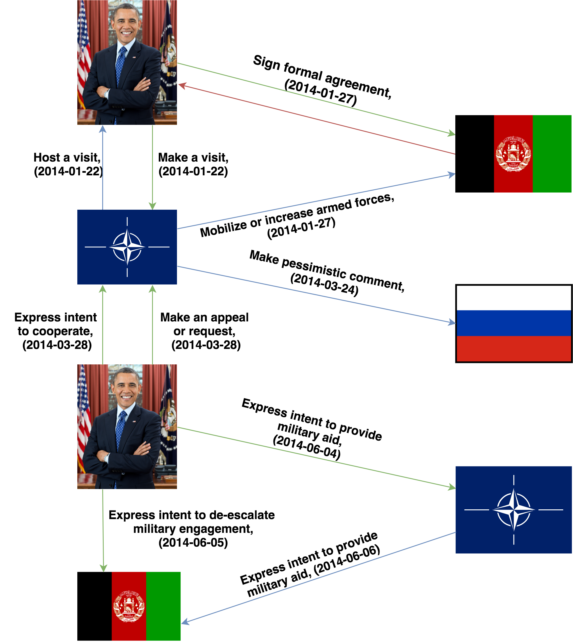
Different events and actions cause relations and entities to evolve over time. For example, Figure 1 illustrates a timeline of relations and events happening in 2014 involving entities like Obama (president of USA at the time), NATO, Afghanistan, and Russia. Here, an agreement between Obama and Afghanistan is happening concurrently with NATO increasing armed forces in Afghanistan; after Obama made a visit to NATO. A few months later, after NATO makes some pessimistic comments towards Russia and Obama wants to de-escalate the conflict, it appears that he provides military aid to NATO, and in turn, NATO provides military aid in Afghanistan.

Temporally-aware KGs are graphs that add a fourth dimension, namely time t, giving the fact a temporal context. Temporal KGs are designed to capture this temporal information and the dynamic nature of real-world facts. While many of the previous works study knowledge graph completion on static KGs, little attention has been given to temporally-aware KGs. Though recent work has begun to solve the temporal link prediction task, these models often utilize a large number of parameters, making them difficult to train (Garcia-Duran, Dumančić, and Niepert 2018; Dasgupta, Ray, and Talukdar 2018; Leblay and Chekol 2018). Furthermore, many use inadequate datasets such as YAGO2 (Hoffart et al. 2013), which are sparse in the time domain, or a time augmented version of FreeBase (Bollacker et al. 2008), where time is appended to some existing facts.

One of the most popular models used to solve the link prediction task involves embedding the KG, that is, mapping entities and relations in the KG to high dimensional vectors, in which each entity and relation mapping considers the structure of the graph as constraints (Bordes et al. 2013; Yang et al. 2014; Lin et al. 2015). These techniques have proven to be the state-of-the-art in modeling static knowledge graphs and inferring new facts from the KG based on the existing ones. Similarly, temporal knowledge graph embedding methods learn an additional mapping for time. Different methods differ based on how they map the elements in the knowledge graph and their scoring function.

In this paper, we propose ChronoR, a novel temporal link prediction model based on $k$-dimensional rotation. We formulate the link prediction problem as learning representations for entities in the knowledge graph and a rotation operator based on each fact’s relation and temporal elements. Further, we show that the proposed scoring function is a generalization of previously used scoring functions for the static KG link prediction task. We also provide insights into the regularization used in other similar models and propose a new regularization method inspired by tensor nuclear norms. Empirical experiments also confirm its advantages. Our experiments on available benchmarks show that ChronoR outperforms previous state-of-the-art methods.

The rest of the paper is organized as follows: Section 2 covers the relevant previous work, Section 3 formally defines the temporal knowledge graph completion problem, in Section 4 we go over the proposed model’s details and learning procedure, Section 5 details the loss and regulation functions, Section 6 discusses the experimental setup, and Section 7 concludes our work.

2 Related Work

2.1 Static KG Embeddings

There has been a substantial amount of research in KG embedding in the non-temporal domain. One of the earliest models, TransE (Bordes et al. 2013), is a translational distance-based model, which embeds the entities h and t, along with relation r, and maps them through the function: h + r = t. There have been several extensions to TransE, including TransH (Wang et al. 2014) which models relations as hyperplanes; TransR (Lin et al. 2015) which embed entities and relations in separate spaces and TransD (Ji et al. 2015) in which two vectors represent each element in a triple in order to represent the elements and construct mapping matrices. Other works, such as DistMult (Yang et al. 2014), represent relations as bilinear functions. ComplEx (Trouillon et al. 2016) extends DistMult to the complex space. RotatE (Sun et al. 2019) also embeds the entities in the complex space, and treats relations as planar rotations. QuatE (Zhang et al. 2019) embeds each element using quaternions.

2.2 Temporal Embeddings

There has been a wide range of approaches to the problem of temporal link prediction (Kazemi and Goel 2020). A straightforward technique is to ignore the timestamps and make a static KB by aggregating links across different times (Liben-Nowell and Kleinberg 2007), then learn a static embedding for each entity. There have been several attempts to improve along this direction by giving more weights to the links that are more recent (Sharan and Neville 2008; Ibrahim and Chen 2015; Ahmed and Chen 2016; Ahmed et al. 2016). In contrast to these methods, (Yao et al. 2016) first learn embeddings for each snapshot of the KB, then aggregate the embeddings by using a weighted average of them. Several techniques have been proposed for the choice of weights of the embedding aggregation, for instance, based on ARIMA (Güneş, Gündüz-Öğüdücü, and Çataltepe 2016) or reinforcement learning (Moradabadi and Meybodi 2017).

Some of the other works to extend sequence models to TKG. (Sarkar, Siddiqi, and Gordon 2007) employs a Kalman filter to learn dynamic node embeddings. (Garcia-Duran, Dumančić, and Niepert 2018) use recurrent neural nets (RNN) to accommodate for temporal data and extend DistMult and TransE to TKG. For each relation, a temporal embedding has been learned by feeding time characters and the static relation embedding to an LSTM. This method only learns dynamic embedding for relations, not entities. Furthermore, (Han et al. 2020) utilize a temporal point process parameterized by a deep neural architecture.

In one of the earliest works to employ representation learning techniques for reasoning over TKGs (Sadeghian et al. 2016), proposed both an embedding method as well as rule mining methods for reasoning over TKGs. Another related work, t-TransE  (Jiang et al. 2016), learns time-based embeddings indirectly by learning the order of time-sensitive relations, such as wasBornIn followed by diedIn. (Esteban et al. 2016) also impose temporal order constraints on their data by adding an element to their quadruple (s,p,o,t:Bool), where Bool indicates if the fact vanishes or continues after time t. However, the model is only demonstrated on medical and sensory data.

Inspired by the success of diachronic word embeddings, some methods have tried to extend them to the TKG problem (Garcia-Duran, Dumančić, and Niepert 2018; Dasgupta, Ray, and Talukdar 2018). Diachronic methods map every (node, timestamp) or (relation, timestamp) pair to a hidden representation. (Goel et al. 2020) learn dynamic embeddings by masking a fraction of the embedding weights with an activation function of frequencies and (Xu et al. 2019) embed the vectors as a direct function of time. Two con-current temporal reasoning methods TeRo (Xu et al. 2020) and TeMP (Wu et al. 2020) are also included in the empirical comparison table in Section 6.

Other methods, like (Ma, Tresp, and Daxberger 2019; Sadeghian et al. 2019b; Jain et al. 2020; Lacroix, Obozinski, and Usunier 2020), do not evolve the embedding of entities over time. Instead, by using a representation for time, learn the temporal behavior. For instance, (Ma, Tresp, and Daxberger 2019) change the scoring function based on the time embedding and (Lacroix, Obozinski, and Usunier 2020) perform tensor decomposition based on the time representation.

3 Problem Definition

In this section, we formally define the problem of temporal knowledge graph completion and specify the notations used throughout the rest of the paper.

We represent scalars with lower case letters $a$, vectors and matrices with bold lower case letters $\bm{a}$, higher order tensors with bold upper case letters $\bm{A}$, and the $i$^th element of a vector $\bm{a}$ as $a_{i}$. We use $\bm{a}\circ\bm{b}$ to denote the element wise product of two vectors and $[\bm{A}|\bm{B}]$ to denote matrix or vector concatenation. We denote the complex norm as $|\cdot|$ and $||\cdot||_{p}$ denotes the vector p-norm; we drop $p$ when $p=2$.

A Temporal Knowledge Graph is referred to a set of quadruples $\mathcal{K}=\{(h,r,t,\tau)\mid h,t\in\mathcal{E},r\in\mathcal{R},\tau\in\mathcal{T}\}$. Each quadruple represents a temporal fact that is true in a world. $\mathcal{E}$ is the set of all entities and $\mathcal{R}$ is the set of all relations in the ontology. The fourth element in each quadruple represents time, which is often discretized. $\mathcal{T}$ represents the set of all possible time stamps.

Temporal Knowledge Graph Completion (temporal link prediction) refers to the problem of completing a TKGE by inferring facts from a given subset of its facts. In this work, we focus on predicting temporal facts within the observed set $\mathcal{T}$, as opposed to the more general problem which also involves forecasting future facts.

4 Temporal KG Representation Learning

In this section, we present a framework for temporal knowledge graph representation learning. Given a TKG, we want to learn representations for entities, relations, and timestamps (e.g., $\bm{h},\bm{r},\bm{t},\bm{\tau}\in\mathds{R}^{n\times k}$) and a scoring function $g(\bm{h},\bm{r},\bm{t},\bm{\tau})\in\mathds{R}$, such that true quadruples receive high scores. Thus, given $g$, the embeddings can be learned by optimizing an appropriate cost function.

Many of the previous works use a variety of different objectives and linear/non-linear operators to adapt static KG completion’s scoring functions to the scoring function $g(\makebox[4.30554pt]{{$\cdot$}})$ in the temporal case (see Section 2).

One example, RotatE (Sun et al. 2019) learns embeddings $\bm{h},\bm{r},\bm{t}\in\mathds{C}^{n}$ by requiring each triplet’s head to fall close to its tail once transformed by an (element-wise) rotation parametrized by the relation vector: $\bm{h}\circ\bm{r}=\bm{t}$, where $|r_{i}|=1$. Thus, RotatE defines $g(h,r,t)=\lambda-||\bm{h}\circ\bm{r}-\bm{t}||$, for some $\lambda\in\mathds{R}$.

Our model is inspired by the success of rotation-based models in static KG completion (Sun et al. 2019; Zhang et al. 2019). For example, to carry out a rotation by an angle $\theta$ in the two dimensional space, one can use the well known Euler’s formula $e^{i\theta}=\cos(\theta)+i\sin(\theta)$, and the fact that if $(x,y)\in\mathds{R}^{2}$ is represented by its dual complex form $z=x+iy\in\mathds{C}$, then $R_{\theta}(x,y)\Leftrightarrow e^{i\theta}z$. We represent rotation by angle $\theta$ in the 2-dimensional space with $R_{\theta}(.)$.

4.1 ChronoR

In this paper, we consider a subset of the group of general linear transformations $\operatorname{GL}(k,\mathds{R})$ over the k-dimensional real space, consisting of rotation and scaling and parametrize the transformation by both time and relation. Intuitively, we expect that for true facts:

$$\operatorname{Q}_{r,\tau}(\bm{h})=\bm{t}$$ (1)

where $\bm{h},\bm{t}\in\mathds{R}^{n\times k}$ and $\operatorname{Q}_{r,\tau}$ represents the (row-wise) linear operator in k-dimensional space, parametrized by $\bm{r}$ and $\bm{\tau}$. Note that any orthogonal matrix $\bm{Q}\in\mathds{R}^{n\times n}$ (i.e., $\bm{Q}^{\mathsf{T}}\bm{Q}=\bm{Q}\bm{Q}^{\mathsf{T}}=I$) is equivalent to a k-dimensional rotation. However, we relax the unit norm constraint, thus extending rotations to a subset of linear operators which also includes scaling.

As previous work has noted, for 2 or 3 dimensional rotations, one can represent $Q$ using complex numbers $\mathds{C}$ and quaternions $\mathds{H}$ ($k=2\text{ and }4$), respectively. Higher dimensional transformations can also be constructed using the Aguilera-Perez Algorithm (Aguilera and Pérez-Aguila 2004) followed by a scalar multiplication.

4.2 Scoring Function

Unlike RotatE, that uses a scoring function based on the Euclidean distance of $\operatorname{Q_{r}}(\bm{h})$ and $\bm{t}$, we propose to use the angle between the two vectors.

Our motivations comes from observations in a variety of previous works (Aggarwal, Hinneburg, and Keim 2001; Zimek, Schubert, and Kriegel 2012) showing that in higher dimensions, the Euclidean norm suffers from the curse of high dimensionality and is not a good measure of the concept of proximity or similarity between vectors. We use the following well-known definition of inner product to define the angle between $\operatorname{Q}_{r,\tau}(\bm{h})$ and $\bm{t}$.

Definition 1.

If $\bm{A}$ and $\bm{B}$ are matrices in $\mathds{R}^{n\times k}$ we define:

$$\left\langle\bm{A},\bm{B}\right\rangle :=\operatorname{tr}(\mathbf{AB^{T}})$$ (2)

$$\cos(\theta) :=\frac{\left\langle\bm{A},\bm{B}\right\rangle}{\sqrt{\left\langle\bm{A},\bm{A}\right\rangle\left\langle\bm{B},\bm{B}\right\rangle}}$$ (3)

Based on the above definition, the angle between two matrices is proportional to their inner product. Hence, we define our scoring function as:

$$g(h,r,t,\tau):=\left\langle\operatorname{Q}_{r,\tau}(\bm{h})\,,\bm{t}\right\rangle$$ (4)

That is, we expect the $\cos$ of the relative angle between $\operatorname{Q}_{r,\tau}(\bm{h})$ and $\bm{t}$ to be higher (i.e., their angle close to $0$) when $(h,r,t,\tau)$ is a true fact in the TKG.

Some of the state of the art work in static KG completion, such as quaternion-based rotations QuatE (Zhang et al. 2019), complex domain tensor factorization (Trouillon et al. 2016), and also recent works on temporal KG completion like TNTComplEx (Lacroix, Obozinski, and Usunier 2020), use a scoring function similar to

$$g(h,r,t) =\operatorname{Re}\{\bm{h}\circ\bm{r}\circ\bm{\bar{t}}\}$$ (5)

$$\text{for }\,\bm{h} ,\bm{r},\bm{t}\in\mathds{C}\text{ or }\mathds{H}$$

and motivate it by the fact that the optimisation function requires the scores to be purely real (Trouillon et al. 2016).

However, it is interesting to note that this scoring method is in fact a special case of Equation 4. The following theorem proves the equivalence for scoring functions used in ComplEx to Equation 4 when $k=2$.

Theorem 1.

If $\bm{a},\bm{b}\in\mathds{C}^{n}$ and $\bm{A},\bm{B}\in\mathds{R}^{n\times 2}$ are their equivalent matrix forms, then $\operatorname{Re}(\bm{a}\circ\bm{\bar{b}})=\left\langle\bm{A},\bm{B}\right\rangle$ (proof in Appendix)

To fully define $g$ we also need to specify how the linear operator $\operatorname{Q}$ is parameterized by $h,\tau$. In the rest of the paper and experiments, we simply concatenate the head and relation embeddings to get $\operatorname{Q}_{r,\tau}=[\bm{r}|\bm{\tau}]$, where $\bm{r}\in\mathds{R}^{n_{r}\times k}$ and $\bm{\tau}\in\mathds{R}^{n_{\tau}\times k}$ are the representations of the fact’s relation and time elements and $n_{r}+n_{\tau}=n$. Since in many real world TKGs, there are a combination of static and dynamic facts, we also allow an extra rotation operator parametrized only by $r$, i.e., an extra term $\bm{R}_{2}\in\mathds{R}^{n\times k}$ in $\operatorname{Q}$ to better represent static facts.

To summarize, our scoring function is defined as:

$$g(h,r,t,\tau):=\left\langle\bm{h}\,\circ[\bm{r}|\bm{\tau}]\,\circ\bm{r}_{2},\bm{t}\right\rangle$$ (6)

where $\bm{r}\in\mathds{R}^{n_{r}\times k}$, $\bm{\tau}\in\mathds{R}^{n_{\tau}\times k}$ and $\bm{r}_{2}\in\mathds{R}^{n\times k}$.

5 Optimization

	ICEWS14				ICEWS05-15				YAGO15K
Model	MRR	Hit@1	Hits@3	Hit@10	MRR	Hit@1	Hit@3	Hit@10	MRR	Hit@1	Hit@3	Hit@10
TransE (2013)	28.0	9.4	-	63.70	29.4	8.4	-	66.30	29.6	22.8	-	46.8
DistMult (2014)	43.9	32.3	-	67.2	45.6	33.7	-	69.1	27.5	21.5	-	43.8
SimpIE (2018)	45.8	34.1	51.6	68.7	47.8	35.9	53.9	70.8	-	-	-	-
ComplEx (2016)	47.0	35.0	54.0	71.0	49.0	37.0	55.0	73.0	36.0	29.0	36.0	54.0
ConT (2018)	18.5	11.7	20.5	31.50	16.4	10.5	18.9	27.20	-	-	-	-
TTransE (2016)	25.5	7.4	-	60.1	27.1	8.4	-	61.6	32.1	23.0	-	51.0
TA-TransE (2018)	27.5	9.5	-	62.5	29.9	9.6	-	66.8	32.1	23.1	-	51.2
HyTE (2018)	29.7	10.8	41.6	65.5	31.6	11.6	44.5	68.1	-	-	-	-
TA-DistMult (2018)	47.7	-	36.3	68.6	47.4	34.6	-	72.8	29.1	21.6	-	47.6
DE-SimpIE (2020)	52.6	41.8	59.2	72.5	51.3	39.2	57.8	74.8	-	-	-	-
TIMEPLEX (2020)	60.40	51.50	-	77.11	63.99	54.51	-	81.81	-	-	-	-
TNTComplEx (2020)	60.72	51.91	65.92	77.17	66.64	58.34	71.82	81.67	35.94	28.49	36.84	53.75
TeRo (concurrent work)	56.2	46.8	62.1	73.2	58.6	46.9	66.8	79.5	-	-	-	-
TeMP-SA (concurrent work)	60.7	48.4	68.4	84.0	68.0	55.3	76.9	91.3	-	-	-	-
ChronoR (k=3)	59.39	49.64	65.40	77.30	68.41	61.06	73.01	82.13	36.50	29.16	37.63	53.53
ChronoR (k=2)	62.53	54.67	66.88	77.31	67.50	59.63	72.29	82.03	36.62	29.18	37.92	53.79

Table 1: Evaluation on the YAGO15k, ICEWS14, and ICEWS05-15 datasets. Results reported for previous related works are the best numbers reported in their respective paper.

Having an appropriate scoring function, one can model the likelihood of any $t_{i}\in\mathcal{E}$, correctly answering the query $g(h,r,?,\tau)$ as:

$$P(t=t_{i}\mid h,r,\tau)=\frac{\operatorname{exp}(g(h,r,t_{i},\tau))}{\sum_{k=1}^{K}\operatorname{exp}(g(h,r,t_{k},\tau))}$$ (7)

and similarly for $P(h=h_{i}\mid r,t,\tau)$.

To learn appropriate model parameters, one can minimize, for each quadruple in the training set, the negative log-likelihood of correct prediction:

$$L(\mathcal{K};\bm{\theta})={\sum}_{(h,r,t,\tau)\in\operatorname{\mathcal{K}}} \left(\sum_{t_{i},h_{i}\in\mathcal{E}}-\log(P_{t_{\scriptscriptstyle i}})-\log(P_{h_{\scriptscriptstyle i}})\right)$$ (8)

where $\bm{\theta}$ represents all the model parameters.

Formulating the loss function following Equation 8 requires computing the denominator of Equation 7 for every fact in the training set of the temporal KG; however it does not require generating negative samples (Armandpour et al. 2019) and has been shown in practice (if computationally feasible - for our experiments’ scale is) to perform better.

5.1 Regularization

Various embedding methods use some form of regularization to improve the model’s generalizability to unseen facts and prevent from overfitting to the training data. TNTComplEx (Lacroix, Obozinski, and Usunier 2020) treats the TKG as an order 3 tensor by unfolding the temporal and predicate mode together and adopts the regularization derived for static KGs in ComplEx (Lacroix, Usunier, and Obozinski 2018). Other methods, for example TIMEPLEX (Jain et al. 2020), use a sample-weighted L2 regularization penalty to prevent overfitting.

We also use the tensor nuclear norm due to its connection to tensor nuclear rank (Friedland and Lim 2018). However, we directly consider the TKG as an order 4 tensor with $\bm{E},\bm{R},\bm{T}$ containing the rank-one coefficients of its decomposition, and where $\bm{E},\bm{R},\bm{T}$ are the tensors containing entity, relation and time embeddings. Based on this connection, we propose the following regularization:

$$\Lambda_{4}(\bm{\theta})=\sum_{(h,r,t,\tau)\in\operatorname{\mathcal{K}}}(||\bm{h}||_{4}^{4}+||\bm{r_{2}}||_{4}^{4}+||[\bm{r}|\bm{\tau}]||_{4}^{4}+||\bm{t}||_{4}^{4})$$ (9)

We empirically compare different regularizations in Section 6 and show that $\Lambda_{4}(\bm{\theta})$ outperforms other methods. We provide the theoretical theorems required to drive Equation 9 in the Appendix.

5.2 Temporal Regularization

In addition, one would like the model to take advantage of the fact that most entities behave smoothly over time. We can capture this smoothness property of real datasets by encouraging the model to learn similar transformations for closer timestamps. Hence, following (Lacroix, Obozinski, and Usunier 2020) and (Sarkar and Moore 2006), we add a temporal smoothness objective to our loss function:

$$\Lambda_{\Upgamma}=\frac{1}{|\mathcal{T}|-1}\sum_{i=1}^{|\mathcal{T}|-1}||\bm{\tau_{i+1}}-\bm{\tau_{i}}||_{4}^{4}$$ (10)

Tuning the hyper-parameter $\lambda_{2}$ is related to the scale of $\Lambda_{\Upgamma}$ and other components of the loss function and finding an appropriate $\lambda_{2}$ can become difficult in practice if each component follows a different scale. Since we are using the 4-norm regularization in $\Lambda_{4}(\bm{\theta})$, we also use the 4-norm for $\Lambda_{\Upgamma}$. Similar phenomenal have been previously explored in other domains. For example, in (Belloni et al. 2014) the authors propose $\sqrt{\text{Lasso}}$, where they use the square root of the MSE component to match the scale of the 1-norm used in the sparsity regularization component of Lasso (Tibshirani 1996) and show improvements in handling the unknown scale in badly behaved systems.

Since we used a 4-norm in $\Lambda_{4}$, we also use the 4-norm for $\Lambda_{\Upgamma}$. We saw that in practice using the same order makes it easier to tune the hyperparameters $\lambda_{1}$ and $\lambda_{2}$ in $\mathcal{L}(\mathcal{K})$.

5.3 Loss Function

To learn the representations for any TKG $\mathcal{K}$, the final training objective is to minimize:

$$\mathcal{L}(\mathcal{K};\theta)=L(\mathcal{K};\bm{\theta})+\lambda_{1}\Lambda_{4}(\bm{\theta})+\lambda_{2}\Lambda_{\Upgamma}$$ (11)

where the first and the second terms encourage an accurate estimation of the edges in the TKG and the third term incorporates the temporal smoothness behaviour.

In the next section, we provide empirical experiments and compare ChronoR to various other benchmarks.

6 Experiments

We evaluate our proposed model for temporal link prediction on temporal knowledge graphs. We tune all the hyper-parameters using a grid search and each dataset’s provided validation set. We tune $\lambda_{1}$ and $\lambda_{2}$ from $\{10^{i}|-3\leq i\leq 1\}$ and the ratio of $\frac{n_{r}}{n_{\tau}}$ from $[0.1,0.9]$ with $0.1$ increments. For a fair comparison, we do not tune the embedding dimension; instead, in each experiment we choose $n$ such that our models have an equal number of parameters to those used in (Lacroix, Obozinski, and Usunier 2020). Table 3, in the Appendix, shows the dimensions used by each model for each of the datasets.

Training was done using mini-batch stochastic gradient descent with AdaGrad and a learning rate of 0.1 with a batch size of 1000 quadruples. We implemented all our models in Pytorch and trained on a single GeForce RTX 2080 GPU. The source code to reproduce the full experimental results will be made public on GitHub.

6.1 Datasets

We evaluate our model on three popular benchmarks for Temporal Knowledge graph completion, namely ICEWS14, ICEWS05-15, and Yago15K. All datasets contain only positive triples. The first two datasets are subsets of Integrated Crisis Early Warning System (ICEWS), which is a very popular knowledge graph used by the community. ICEWS14 is collected from 01/01/2014 to 12/31/2014, while ICEWS15-05 is the subset occurring between 01/01/2005 and 12/31/2015. Both datasets have timestamps for every fact with a temporal granularity of 24 hours. It is worth mentioning that these datasets are selected such that they only include the most frequently occurring entities (in both head and tail). Below are examples from ICEWS14:

(John Kerry, Praise or endorse,        Lawmaker (Iraq), 2014-10-18)(Iraq, Receive deployment of peacekeepers,        Iran, 2014-07-05)(Japan, Engage in negotiation,        South Korea, 2014-02-18)

To create YAGO15K, Garcia-Duran, Dumančić, and Niepert (2018) aligned the entities in FB15K (Bordes et al. 2013) with those from YAGO, which contains temporal information. The final dataset is the result of all facts with successful alignment. It is worth noting that since YAGO does not have temporal information for all facts, this dataset is also temporally incomplete and more challenging. Below are examples from this dataset:

(David_Beckham, isAffiliatedTo, Man_U)(David_B, isAffiliatedTo, Paris_SG)(David_B, isMarriedTo, Victoria_Beckham,                 occursSince, "1999-##-##")

	ICEWS14	ICEWS05-15	YAGO15k
Entities	7,128	10,488	15,403
Relations	230	251	34
Timestamps	365	4,017	198
Facts	90,730	479,329	138,056
Time Span	2014	2005 - 2015	1513 - 2017

Table 2: Statistics for the various experimental datasets.

	ICEWS14	ICEWS05-15	YAGO15k
ChronoR k=2	1600	1350	1900
ChronoR k=3	800	700	950

Table 3: The embedding dimension (n) for each dataset used in our experiments.

To adapt YAGO15 to our model, following (Lacroix, Obozinski, and Usunier 2020), for each fact we group the relations occureSince/occureUntil together, in turn doubling our relation size. Note that this does not effect the evaluation protocol. Table 2, summarizes the statistics of used temporal KG benchmarks.

Figure 2: Comparison of various regularizers with different weights on a ChronoR(k=2) trained on ICEWS14.

6.2 Evaluation Metrics and Baselines

We follow the experimental set-up described in (Garcia-Duran, Dumančić, and Niepert 2018) and (Goel et al. 2020). For each quadruple $(h,r,t,\tau)$ in the test set, we fill $(h,r,?,\tau)$ and $(?,r,t,\tau)$ by scoring and sorting all possible entities in $\mathscr{E}$. We report Hits@k for $k=1,3,10$ and filtered Mean Reciprocal Rank (MRR) for all datasets. Please see (Nickel, Rosasco, and Poggio 2016) for more details about filtered MRR.

We use baselines from both static and temporal KG embedding models. From the static KG embedding models, we use TransE, DistMult, SimplE, and ComplEx. These models ignore the timing information. It is worth noting that when evaluating these models on temporal KGs in the filtered setting, for each test quadruple, one must filter previously seen entities according to the fact and its time stamp, for a fair comparison.

To the best of our knowledge, we compare against every previously published temporal KG embedding models that have been evaluated on these datasets, which we discussed the details of in Section 2.

6.3 Results

In this section we analyze and perform a quantitative comparison of our model and previous state-of-the-art ones. We also experimentally verify the advantage of using Equation 9 for learning temporal embeddings.

Table 2 demonstrates link prediction performance comparison on all datasets. ChronoR consistently outperforms all competitors in terms of link prediction MRR and is greater than or equal to the previous work in terms of Hits@10 metric.

Our experiments with rotations in 3-dimensions show an improvement over ICEWS05-15, but lower performances compared to planar rotations on the other two datasets. We believe this is due to the more complex nature of this dataset (the higher number of relations and timestamps) compared to YAGO15K and ICEWS14. We do not see any significant gain on these three datasets using higher dimensional rotations. Similar to the observations in some static KG benchmarks (Toutanova and Chen 2015), this might suggest the need for more sophisticated detests. However, we leave further studying of these datasets for future work.

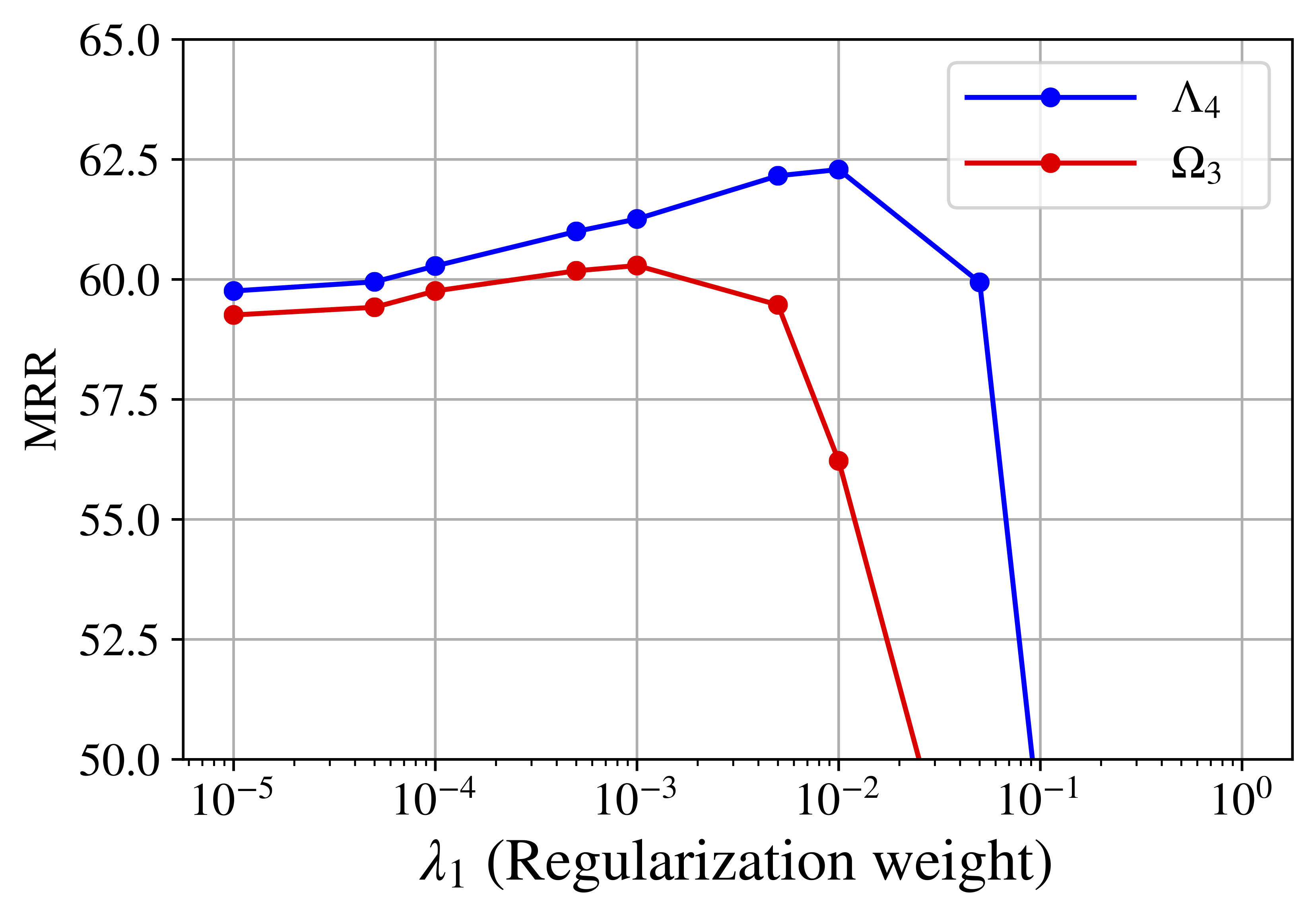
In Figure 2, we plot a detailed comparison of our proposed regularizer to $\Omega_{3}$, the regularizer used in TNTComplEx (Lacroix, Obozinski, and Usunier 2020). $\Omega_{3}$, is a variational form of the nuclear 3-norm and is based on folding the TKG (as a 4-tensor) on its relation and temporal axis to get an order 3 tensor.

We drive $\Lambda_{4}$ by directly linking the scoring function to the 4-tensors factorization and show that it is the natural regularizer to use when penalizing by tensor nuclear norm. Note that $\Lambda_{4}$ increases MRR by 2 points and carefully selecting regularization weight can increase MRR up to 7 points.

7 Conclusion

We propose a novel k-dimensional rotation based embedding model to learn useful representations from temporal Knowledge graphs. Our method takes into account the change in entities and relations with respect to time. The temporal dynamics of both subject and object entities are captured by transforming them in the embedding space through rotation and scaling operations. Our work generalizes and adopts prior rotation based models in static KGs to the temporal domain. Moreover, we highlight and establish previously unexplored connections between prior scoring and regularization functions. Experimentally, we showed that ChronoR provides state-of-the-art performance on a variety of benchmark temporal KGs and that it can model the dynamics of temporal and relational patterns while being very economical in the number of its parameters. In future work, we will investigate combining other geometrical transformations and rotations and also explore other regularization techniques as well as closely examine the current temporal datasets as discussed in the experiment section.

References

- Abdelaziz et al. (2017) Abdelaziz, I.; Fokoue, A.; Hassanzadeh, O.; Zhang, P.; and Sadoghi, M. 2017. Large-scale structural and textual similarity-based mining of knowledge graph to predict drug–drug interactions. Journal of Web Semantics 44: 104–117.
- Aggarwal, Hinneburg, and Keim (2001) Aggarwal, C. C.; Hinneburg, A.; and Keim, D. A. 2001. On the surprising behavior of distance metrics in high dimensional space. In International conference on database theory, 420–434. Springer.
- Aguilera and Pérez-Aguila (2004) Aguilera, A.; and Pérez-Aguila, R. 2004. General n-dimensional rotations .
- Ahmed and Chen (2016) Ahmed, N. M.; and Chen, L. 2016. An efficient algorithm for link prediction in temporal uncertain social networks. Information Sciences 331: 120–136.
- Ahmed et al. (2016) Ahmed, N. M.; Chen, L.; Wang, Y.; Li, B.; Li, Y.; and Liu, W. 2016. Sampling-based algorithm for link prediction in temporal networks. Information Sciences 374: 1–14.
- Armandpour et al. (2019) Armandpour, M.; Ding, P.; Huang, J.; and Hu, X. 2019. Robust negative sampling for network embedding. In Proceedings of the AAAI Conference on Artificial Intelligence, volume 33, 3191–3198.
- Auer et al. (2007) Auer, S.; Bizer, C.; Kobilarov, G.; Lehmann, J.; Cyganiak, R.; and Ives, Z. 2007. Dbpedia: A nucleus for a web of open data. In The semantic web.
- Belloni et al. (2014) Belloni, A.; Chernozhukov, V.; Wang, L.; et al. 2014. Pivotal estimation via square-root lasso in nonparametric regression. The Annals of Statistics 42(2): 757–788.
- Biega, Kuzey, and Suchanek (2013) Biega, J.; Kuzey, E.; and Suchanek, F. M. 2013. Inside YAGO2s: a transparent information extraction architecture. In Proceedings of the 22nd International Conference on World Wide Web.
- Blog (2012) Blog, G. 2012. Introducing the knowledge graph: thing, not strings. Introducing the Knowledge Graph: things, not strings .
- Bollacker et al. (2008) Bollacker, K.; Evans, C.; Paritosh, P.; Sturge, T.; and Taylor, J. 2008. Freebase: a collaboratively created graph database for structuring human knowledge. In Proceedings of the 2008 ACM SIGMOD international conference on Management of data.
- Bordes et al. (2013) Bordes, A.; Usunier, N.; Garcia-Duran, A.; Weston, J.; and Yakhnenko, O. 2013. Translating embeddings for modeling multi-relational data. In Advances in neural information processing systems.
- Burgun and Bodenreider (2001) Burgun, A.; and Bodenreider, O. 2001. Comparing terms, concepts and semantic classes in WordNet and the Unified Medical Language System. In Proceedings of the NAACL’2001 Workshop,“WordNet and Other Lexical Resources: Applications, Extensions and Customizations.
- Cao et al. (2019) Cao, Y.; Wang, X.; He, X.; Hu, Z.; and Chua, T.-S. 2019. Unifying knowledge graph learning and recommendation: Towards a better understanding of user preferences. In The world wide web conference.
- Carlson et al. (2010) Carlson, A.; Betteridge, J.; Kisiel, B.; Settles, B.; Hruschka Jr, E. R.; and Mitchell, T. M. 2010. Toward an architecture for never-ending language learning. In Aaai.
- Dasgupta, Ray, and Talukdar (2018) Dasgupta, S. S.; Ray, S. N.; and Talukdar, P. 2018. HyTE: Hyperplane-based Temporally aware Knowledge Graph Embedding. In Proceedings of the 2018 Conference on Empirical Methods in Natural Language Processing.
- Esteban et al. (2016) Esteban, C.; Tresp, V.; Yang, Y.; Baier, S.; and Krompaß, D. 2016. Predicting the co-evolution of event and knowledge graphs. In 2016 19th International Conference on Information Fusion (FUSION), 98–105. Ieee.
- Etzioni et al. (2011) Etzioni, O.; Fader, A.; Christensen, J.; Soderland, S.; and Mausam, M. 2011. Open information extraction: The second generation. In IJCAI.
- Friedland and Lim (2018) Friedland, S.; and Lim, L.-H. 2018. Nuclear norm of higher-order tensors. Mathematics of Computation .
- Garcia-Duran, Dumančić, and Niepert (2018) Garcia-Duran, A.; Dumančić, S.; and Niepert, M. 2018. Learning Sequence Encoders for Temporal Knowledge Graph Completion. In Proceedings of the 2018 Conference on Empirical Methods in Natural Language Processing, 4816–4821.
- Goel et al. (2020) Goel, R.; Kazemi, S.; Brubaker, M. A.; and Poupart, P. 2020. Diachronic Embedding for Temporal Knowledge Graph Completion. In Thirty-Fourth AAAI Conference on Artificial Intelligence.
- Güneş, Gündüz-Öğüdücü, and Çataltepe (2016) Güneş, İ.; Gündüz-Öğüdücü, Ş.; and Çataltepe, Z. 2016. Link prediction using time series of neighborhood-based node similarity scores. Data Mining and Knowledge Discovery 30(1): 147–180.
- Han et al. (2020) Han, Z.; Wang, Y.; Ma, Y.; Guünnemann, S.; and Tresp, V. 2020. The Graph Hawkes Network for Reasoning on Temporal Knowledge Graphs. arXiv preprint arXiv:2003.13432 .
- Hao et al. (2017) Hao, Y.; Zhang, Y.; Liu, K.; He, S.; Liu, Z.; Wu, H.; and Zhao, J. 2017. An end-to-end model for question answering over knowledge base with cross-attention combining global knowledge. In Proceedings of the 55th Annual Meeting of the Association for Computational Linguistics (Volume 1: Long Papers), 221–231.
- Hoffart et al. (2013) Hoffart, J.; Suchanek, F. M.; Berberich, K.; and Weikum, G. 2013. YAGO2: A spatially and temporally enhanced knowledge base from Wikipedia. Artificial Intelligence .
- Ibrahim and Chen (2015) Ibrahim, N. M. A.; and Chen, L. 2015. Link prediction in dynamic social networks by integrating different types of information. Applied Intelligence 42(4): 738–750.
- Jain et al. (2020) Jain, P.; Rathi, S.; Chakrabarti, S.; et al. 2020. Temporal Knowledge Base Completion: New Algorithms and Evaluation Protocols. arXiv preprint arXiv:2005.05035 .
- Ji et al. (2015) Ji, G.; He, S.; Xu, L.; Liu, K.; and Zhao, J. 2015. Knowledge graph embedding via dynamic mapping matrix. In Proceedings of the 53rd Annual Meeting of the Association for Computational Linguistics and the 7th International Joint Conference on Natural Language Processing (Volume 1: Long Papers), volume 1, 687–696.
- Jiang et al. (2016) Jiang, T.; Liu, T.; Ge, T.; Sha, L.; Li, S.; Chang, B.; and Sui, Z. 2016. Encoding temporal information for time-aware link prediction. In Proceedings of the 2016 Conference on Empirical Methods in Natural Language Processing, 2350–2354.
- Kazemi and Goel (2020) Kazemi, S. M.; and Goel, R. 2020. Representation Learning for Dynamic Graphs: A Survey. Journal of Machine Learning Research 21: 1–73.
- Lacroix, Obozinski, and Usunier (2020) Lacroix, T.; Obozinski, G.; and Usunier, N. 2020. Tensor Decompositions for temporal knowledge base completion. ICLR .
- Lacroix, Usunier, and Obozinski (2018) Lacroix, T.; Usunier, N.; and Obozinski, G. 2018. Canonical tensor decomposition for knowledge base completion. arXiv preprint arXiv:1806.07297 .
- Leblay and Chekol (2018) Leblay, J.; and Chekol, M. W. 2018. Deriving validity time in knowledge graph. In Companion of the The Web Conference 2018 on The Web Conference 2018. International World Wide Web Conferences Steering Committee.
- Liben-Nowell and Kleinberg (2007) Liben-Nowell, D.; and Kleinberg, J. 2007. The link-prediction problem for social networks. Journal of the American society for information science and technology 58(7): 1019–1031.
- Lin et al. (2015) Lin, Y.; Liu, Z.; Sun, M.; Liu, Y.; and Zhu, X. 2015. Learning entity and relation embeddings for knowledge graph completion. In Twenty-ninth AAAI conference on artificial intelligence.
- Ma, Tresp, and Daxberger (2019) Ma, Y.; Tresp, V.; and Daxberger, E. A. 2019. Embedding models for episodic knowledge graphs. Journal of Web Semantics 59: 100490.
- Mahdisoltani, Biega, and Suchanek (2013) Mahdisoltani, F.; Biega, J.; and Suchanek, F. M. 2013. Yago3: A knowledge base from multilingual wikipedias. In CIDR.
- Moradabadi and Meybodi (2017) Moradabadi, B.; and Meybodi, M. R. 2017. A novel time series link prediction method: Learning automata approach. Physica A: Statistical Mechanics and its Applications 482: 422–432.
- Nickel, Rosasco, and Poggio (2016) Nickel, M.; Rosasco, L.; and Poggio, T. 2016. Holographic embeddings of knowledge graphs. In Thirtieth Aaai conference on artificial intelligence.
- Sadeghian et al. (2019a) Sadeghian, A.; Armandpour, M.; Ding, P.; and Wang, D. Z. 2019a. DRUM: End-To-End Differentiable Rule Mining On Knowledge Graphs. In Wallach, H.; Larochelle, H.; Beygelzimer, A.; d'Alché-Buc, F.; Fox, E.; and Garnett, R., eds., Advances in Neural Information Processing Systems, volume 32. Curran Associates, Inc. URL https://proceedings.neurips.cc/paper/2019/file/0c72cb7ee1512f800abe27823a792d03-Paper.pdf.
- Sadeghian et al. (2019b) Sadeghian, A.; Minaee, S.; Partalas, I.; Li, X.; Wang, D. Z.; and Cowan, B. 2019b. Hotel2vec: Learning Attribute-Aware Hotel Embeddings with Self-Supervision. arXiv preprint arXiv:1910.03943 .
- Sadeghian et al. (2016) Sadeghian, A.; Rodriguez, M.; Wang, D. Z.; and Colas, A. 2016. Temporal reasoning over event knowledge graphs.
- Sang et al. (2018) Sang, S.; Yang, Z.; Wang, L.; Liu, X.; Lin, H.; and Wang, J. 2018. SemaTyP: a knowledge graph based literature mining method for drug discovery. BMC bioinformatics 19(1): 193.
- Sarkar and Moore (2006) Sarkar, P.; and Moore, A. W. 2006. Dynamic social network analysis using latent space models. In Advances in Neural Information Processing Systems, 1145–1152.
- Sarkar, Siddiqi, and Gordon (2007) Sarkar, P.; Siddiqi, S. M.; and Gordon, G. J. 2007. A latent space approach to dynamic embedding of co-occurrence data. In Artificial Intelligence and Statistics, 420–427.
- Sharan and Neville (2008) Sharan, U.; and Neville, J. 2008. Temporal-relational classifiers for prediction in evolving domains. In 2008 Eighth IEEE International Conference on Data Mining, 540–549. IEEE.
- Sun et al. (2019) Sun, Z.; Deng, Z.-H.; Nie, J.-Y.; and Tang, J. 2019. Rotate: Knowledge graph embedding by relational rotation in complex space. arXiv preprint arXiv:1902.10197 .
- Tibshirani (1996) Tibshirani, R. 1996. Regression shrinkage and selection via the lasso. Journal of the Royal Statistical Society: Series B (Methodological) 58(1): 267–288.
- Toutanova and Chen (2015) Toutanova, K.; and Chen, D. 2015. Observed versus latent features for knowledge base and text inference. In Proceedings of the 3rd Workshop on Continuous Vector Space Models and their Compositionality, 57–66.
- Trouillon et al. (2016) Trouillon, T.; Welbl, J.; Riedel, S.; Gaussier, É.; and Bouchard, G. 2016. Complex embeddings for simple link prediction. International Conference on Machine Learning (ICML).
- Wang et al. (2014) Wang, Z.; Zhang, J.; Feng, J.; and Chen, Z. 2014. Knowledge graph embedding by translating on hyperplanes. In Twenty-Eighth AAAI conference on artificial intelligence.
- Wu et al. (2020) Wu, J.; Cao, M.; Cheung, J. C. K.; and Hamilton, W. L. 2020. TeMP: Temporal Message Passing for Temporal Knowledge Graph Completion. arXiv preprint arXiv:2010.03526 .
- Xiong, Power, and Callan (2017) Xiong, C.; Power, R.; and Callan, J. 2017. Explicit semantic ranking for academic search via knowledge graph embedding. In Proceedings of the 26th international conference on world wide web, 1271–1279.
- Xu et al. (2019) Xu, C.; Nayyeri, M.; Alkhoury, F.; Lehmann, J.; and Yazdi, H. S. 2019. Temporal knowledge graph embedding model based on additive time series decomposition. arXiv preprint arXiv:1911.07893 .
- Xu et al. (2020) Xu, C.; Nayyeri, M.; Alkhoury, F.; Yazdi, H. S.; and Lehmann, J. 2020. TeRo: A Time-aware Knowledge Graph Embedding via Temporal Rotation. arXiv preprint arXiv:2010.01029 .
- Yang and Mitchell (2017) Yang, B.; and Mitchell, T. 2017. Leveraging knowledge bases in lstms for improving machine reading. Proceedings of the 55th Annual Meeting of the Association for Computational Linguistics .
- Yang et al. (2014) Yang, B.; Yih, W.-t.; He, X.; Gao, J.; and Deng, L. 2014. Embedding entities and relations for learning and inference in knowledge bases. arXiv preprint arXiv:1412.6575 .
- Yao et al. (2016) Yao, L.; Wang, L.; Pan, L.; and Yao, K. 2016. Link prediction based on common-neighbors for dynamic social network. Procedia Computer Science 83: 82–89.
- Yates et al. (2007) Yates, A.; Banko, M.; Broadhead, M.; Cafarella, M. J.; Etzioni, O.; and Soderland, S. 2007. Textrunner: open information extraction on the web. In (NAACL-HLT).
- Zhang et al. (2016) Zhang, F.; Yuan, N. J.; Lian, D.; Xie, X.; and Ma, W.-Y. 2016. Collaborative knowledge base embedding for recommender systems. In Proceedings of the 22nd ACM SIGKDD international conference on knowledge discovery and data mining, 353–362.
- Zhang et al. (2019) Zhang, S.; Tay, Y.; Yao, L.; and Liu, Q. 2019. Quaternion knowledge graph embeddings. In Advances in Neural Information Processing Systems, 2735–2745.
- Zhou, Sadeghian, and Wang (2019) Zhou, X.; Sadeghian, A.; and Wang, D. Z. 2019. Mining Rules Incrementally over Large Knowledge Bases. In Proceedings of the 2019 SIAM International Conference on Data Mining, 154–162. SIAM.
- Zimek, Schubert, and Kriegel (2012) Zimek, A.; Schubert, E.; and Kriegel, H.-P. 2012. A survey on unsupervised outlier detection in high-dimensional numerical data. Statistical Analysis and Data Mining: The ASA Data Science Journal 5(5): 363–387.