A framework for energy and carbon footprint analysis of distributed and federated edge learning

Abstract

Recent advances in distributed learning raise environmental concerns due to the large energy needed to train and move data to/from data centers. Novel paradigms, such as federated learning (FL), are suitable for decentralized model training across devices or silos that simultaneously act as both data producers and learners. Unlike centralized learning (CL) techniques, relying on big-data fusion and analytics located in energy hungry data centers, in FL scenarios devices collaboratively train their models without sharing their private data. This article breaks down and analyzes the main factors that influence the environmental footprint of FL policies compared with classical CL/Big-Data algorithms running in data centers. The proposed analytical framework takes into account both learning and communication energy costs, as well as the carbon equivalent emissions; in addition, it models both vanilla and decentralized FL policies driven by consensus. The framework is evaluated in an industrial setting assuming a real-world robotized workplace. Results show that FL allows remarkable end-to-end energy savings ($30\%\div 40\%$) for wireless systems characterized by low bit/Joule efficiency ($50$ kbit/Joule or lower). Consensus-driven FL does not require the parameter server and further reduces emissions in mesh networks ($200$ kbit/Joule). On the other hand, all FL policies are slower to converge when local data are unevenly distributed (often 2x slower than CL). Energy footprint and learning loss can be traded off to optimize efficiency.

I Introduction

Recent advances in machine learning (ML) have revolutionized many domains and industrial scenarios. However, such improvements have been achieved at the cost of large computational and communication resources, resulting in significant energy and CO2 (carbon) footprints. Traditional centralized learning (CL) requires all training procedures to be conducted inside data centers [1] that are in charge of collecting training data from data producers (e.g. sensors, machines and personal devices), fusing large datasets, and continuously learning from them [2]. Data centers are thus energy-hungry and responsible for significant carbon emissions that amount to about $15$% of the global emissions of the entire Information and Communication Technology (ICT) ecosystem [3].

An emerging alternative to centralized architectures is federated learning (FL) [4, 5]. Under FL, ML model parameters, e.g. weights and biases $\mathbf{W}$ of Deep Neural Networks (DNN), are collectively optimized across several resource-constrained edge/fog devices, that act as both data producers and local learners. FL distributes the computing task across many devices characterized by low-power consumption profiles, compared with data centers, and owning small datasets [2].

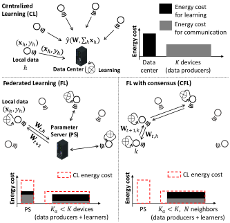
Figure 1: Centralized Learning (CL), Federated Learning (FL) with Parameter Server (PS), namely federated averaging (FA), and FL with consensus (i.e., without PS), namely consensus-driven federated learning (CFL).

As shown in Fig. 1, using FL policies, such as federated averaging [5], allows devices to learn a local model under the orchestration of a centralized parameter server (PS). The PS fuses the received local models to obtain a global model that is fed back to the devices. PS functions are substantially less energy-hungry compared to CL and can be implemented at the network edge. This suggests that FL could bring significant reduction in the energy footprints, as the consumption is distributed across devices obviating the need for a large infrastructure for cooling or power delivery. However, vanilla FL architectures still leverage the server-client architecture which not only represents a single-point of failure, but also lacks scalability and, if not optimized, can further increase the energy footprint. To tackle these drawbacks, recent developments in FL architectures target fully decentralized solutions relying solely on in-network processing, thus replacing PS functions with a consensus-based federation model. In consensus-based FL (CFL), the participating devices mutually exchange their local ML model parameters, possibly via mesh, or device-to-device (D2D) communication links [2], and implement distributed weighted averaging [6, 7, 8]. Devices might be either co-located in the same geographic area or distributed.

Contributions: the paper develops a novel framework for the analysis of energy and carbon footprints in distributed ML, including, for the first time, comparisons and trade-off considerations about vanilla FL, consensus-based (CFL) and data center based centralized learning. Despite an initial attempt to assess the carbon footprint for FL [3], the problem of quantifying an end-to-end analysis of the energy footprint still remains unexplored. To fill this void, we develop an end-to-end framework and validate it using real world data.

The paper is organized as follows: Sections II and III describe the framework for energy consumption and carbon footprint evaluation of different FL strategies, and the impact of energy efficiency in terms of communication and computing costs. In Section IV, we consider a case study in a real-world industrial workplace targeting the learning of a ML model to localize human operators in a human-robot cooperative manufacturing plant. Carbon emissions are quantified and discussed in continuous industrial workflow applications requiring periodic model training updates.

II Energy footprint modeling framework

The proposed framework provides insights into how different components of the FL architecture, i.e. the local learners, the core network and the PS, contribute to the energy bill. The learning system consists of $K$ devices and one data center ($k=0$). Each device $k>0$ has a dataset $\mathcal{E}_{k}$ of (labeled) examples $(\mathbf{x}_{h},y_{h})$ that are typically collected independently. The objective of the learning system is to train a DNN model $\hat{y}(\mathbf{W};\mathbf{x})$ that transforms the input data $\mathbf{x}$ into the desired outputs $\hat{y}\in\left\{y_{c}\right\}_{c=1}^{C}$ where $C$ is the number of the output classes. Model parameters are specified by the matrix $\mathbf{W}$ [5]. The training system uses the examples in $\bigcup_{k=1}^{K}\mathcal{E}_{k}$ to minimize the loss function $\xi(\mathbf{x}_{h},y_{h}|\mathbf{W})$ iteratively, over a pre-defined number $n$ of learning rounds.

Considering a device $k$, the total amount of energy consumed by the learning process can be broken down into computing and communication components. The energy cost is thus modelled as a function of the energy $E_{k}^{(\mathrm{C})}$ due to computing per learning round, and the energy $E_{k,h}^{(\mathrm{T})}$ per correctly received/transmitted bit over the wireless link ($k,h$). In particular, the latter can be further broken down into uplink (UL) communication ($E_{k,0}^{(\mathrm{T})}$) with the data center (or the PS), and downlink (DL) communication ($E_{0,k}^{(\mathrm{T})}$), from the PS to the device. The energy cost for communication includes the power dissipated in the RF front-end, in the conversion, baseband processing and transceiver stages. We neglect the cost of on-off radio switching. In addition, communication energy costs are quantified on average, as routing through the radio access and the core network can vary (but might be assumed as stationary apart from failures or replacements). Finally, the energy $E_{k}^{(\mathrm{C})}$ for computing includes the cost of the learning round, namely the local gradient-based optimizer and data storage. In what follows, we quantify the energy cost of model training implemented either inside the data center (CL) or distributed across multiple devices (FL). Numerical examples are given in Table I and in the case study in Section IV.

II-A Centralized Learning (CL)

Under CL, model training is carried out inside the data center $k=0$, while the energy cost per round $E_{0}^{(\mathrm{C})}=P_{0}\cdot T_{0}\cdot B$ depends on the GPU/CPU power consumption $P_{0}$ [3], the time span $T_{0}$ required for processing an individual batch of data, i.e. minimizing the loss $\xi(\cdot|\mathbf{W})$, and the number $B$ of batches per round. We neglect here the cost of initial dataset loading since it is a one-step process. For $n=n(\overline{\xi})$ rounds, and a target loss $\overline{\xi}$, the total, end-to-end, energy in Joule [J] is given by:

$$E_{CL}(\xi)=\gamma\cdot n\cdot E_{0}^{(\mathrm{C})}+\sum_{k=1}^{K}b(\mathcal{E}_{k})\cdot E_{k,0}^{(\mathrm{T})},$$ (1)

where $\gamma$ is the Power Usage Effectiveness (PUE) of the considered data center [10, 11]. The cost for UL communication for data fusion, $\sum_{k=1}^{K}b(\mathcal{E}_{k})\cdot E_{k,0}^{(\mathrm{T})}$, scales with the data size $b(\mathcal{E}_{k})$ of the $k$-th local database $\mathcal{E}_{k}$ and the number of devices $K$. PUE $\gamma>1$ accounts for the additional power consumed by the data center infrastructure for data storage, power delivery and cooling; values are typically $\gamma=1.1\div 1.8$ [11].

TABLE I: Computing costs and communication energy efficiency (EE) values for FL energy/carbon footprint evaluation.

Parameters	Data center/PS ($k=0$)	Devices ($k\geq 1$)
Comp. $P_{k}$:	$140\,\mathrm{W}$(CPU)$\,+\,42\,\mathrm{W}$(GPU)	$5.1\,\mathrm{W}$ (CPU)
Batch time $T_{k}$:	$20$ ms	$190$ ms
Batches $B$:	$3$	$3$
Raw data size:	$K\cdot b(\mathcal{E}_{k})$ MB	$b(\mathcal{E}_{k})\simeq 30$ MB
Model size:	$b(\mathbf{W})=290$ KB	$b(\mathbf{W})=290$ KB
PUE $\gamma$:	$1.67$	$1$
Utilization $\beta$:	$0.1$ (model averaging)
ML model:	DeepMind [9], $5$ layers, $C=6$. Optimizer: Adam
Comm. $\mathrm{EE}$:	Downlink (DL):	Uplink (UL):
	$\mathrm{EE_{D}}=0.02\div 1$Mb/J	$\mathrm{EE_{U}=0.02\div 1}$Mb/J
		Mesh or D2D (M):
		$\mathrm{EE_{M}=0.01\div 1}$Mb/J
Comp. $\mathrm{EE}$:	$\mathrm{EE_{C}}=0.9$ round/J	$\mathrm{\tfrac{EE_{C}}{\varphi}}$ round/J, $\varphi=0.22$

TABLE II: Communication and computing carbon footprints.

	Communication $C_{\mathrm{C}}$	Computing $C_{\mathrm{L}}$	Carbon footprint
CL (data center):	$\sum_{k=1}^{K}b(\mathcal{E}_{k})\cdot\frac{\mathrm{CI}_{k}}{\mathrm{EE_{U}}}$	$n\cdot\gamma\cdot\frac{\mathrm{CI}_{0}}{\mathrm{EE_{C}}}$	$C_{\mathrm{CL}}=C_{\mathrm{C}}+C_{\mathrm{L}}$
FL (with PS): $K_{a}\leq K$	$n\cdot b(\mathbf{W})\cdot\left(\sum_{k=1}^{K_{a}}\frac{\mathrm{CI}_{k}}{\mathrm{EE_{U}}}+\gamma\cdot K\cdot\frac{\mathrm{CI}_{0}}{\mathrm{EE_{D}}}\right)$	$n\cdot\left(\sum_{k=1}^{K_{a}}\frac{\varphi\cdot\mathrm{CI}_{k}}{\mathrm{EE_{C}}}+\beta\cdot\gamma\cdot\frac{\mathrm{CI}_{0}}{\mathrm{EE_{C}}}\right)$	$C_{\mathrm{FL}}=C_{\mathrm{C}}+C_{\mathrm{L}}$
CFL : $K_{a}\leq K$, $N\geq 1$	$n\cdot b(\mathbf{W})\cdot\left(\sum_{k=1}^{K_{a}}\frac{N\cdot\mathrm{CI}_{k}}{\mathrm{EE_{M}}}\right)$,	$n\cdot\sum_{k=1}^{K_{a}}\frac{\varphi\cdot\mathrm{CI}_{k}}{\mathrm{EE_{C}}}$	$C_{\mathrm{CFL}}=C_{\mathrm{C}}+C_{\mathrm{L}}$

II-B Federated Learning (FL)

Unlike CL, FL distributes the learning process across a selected subset $\mathcal{N}_{t}$ of $K_{a}<K$ active devices as shown in Fig. 1. At each round $t$, the local dataset $\mathcal{E}_{k}$ is used to train a local model $\mathbf{W}_{k,t}$, in order to minimize the local loss $\xi_{k}$ as $\mathbf{W}_{k,t}=\underset{\mathbf{W}}{\mathrm{arg}\mathrm{min}}\thinspace\xi_{k}(\cdot|\mathbf{W})$. The local model is then forwarded to the PS [5] over the UL. The PS is in charge of updating the global model $\mathbf{W}_{t+1}$ for the following round $t+1$ through the aggregation of the $K_{a}$ received models [4]: $\mathbf{W}_{t+1}=\tfrac{1}{K_{a}}\sum_{k\in\mathcal{N}_{t}}\Gamma_{k}\cdot\mathbf{W}_{k,t}$, with $\Gamma_{k}=\tfrac{Q_{k}}{Q}$ and ($Q_{k},Q$) being the number of local and global examples, respectively. The new model $\mathbf{W}_{t+1}$ is finally sent back to the devices over the DL. Other strategies are discussed in [5]. Notice that, while $K_{a}$ active devices run the local optimizer and share the local model with the PS on the assigned round, the remaining $K-K_{a}$ devices have their computing hardware turned off, while the communication interface is powered on to decode the updated global model.

For $n$ rounds, now consisting of learning and communication tasks, the total end-to-end energy includes both devices and PS consumption, namely:

$$E_{FL}(\xi)={} \gamma\cdot n\cdot\beta\cdot E_{0}^{(\mathrm{C})}\,+$$ (2)

$$+\gamma\cdot\sum_{t=1}^{n}\sum_{k=1}^{K}b(\mathbf{W})\cdot E_{0,k}^{(\mathrm{T})}\,+$$

$$+\sum_{t=1}^{n}\sum_{k\in\mathcal{N}_{t}}\left[E_{k}^{(\mathrm{C})}+b(\mathbf{W})\cdot E_{k,0}^{(\mathrm{T})}\right]\,.$$

PS energy is given by $\beta\cdot E_{0}^{(\mathrm{C})}$ and depends on the time, $\beta T_{0}$, needed for model averaging. This is considerably smaller than the batch time $T_{0}$ at the data center (i.e., $\beta\ll 1$). The energy cost per round for device $k$ is due to the local optimization over the data batches $\mathcal{E}_{k}$: $E_{k}^{(\mathrm{C})}=P_{k}\cdot B\cdot T_{k}$. Notice that, while data centers employ high-performance CPUs, GPUs or other specialized hardware (e.g., NPUs or TPUs), the devices are usually equipped with embedded low-consumption CPUs or microcontrollers. Thus, it is reasonable to assume $E_{k}^{(\mathrm{C})}<E_{0}^{(\mathrm{C})}$. Model size $b(\mathbf{W})$ quantifies the size in bits of model parameters to be exchanged, which is typically much smaller compared with the raw data [5]: $b(\mathbf{W})\ll b(\mathcal{E}_{k})$. In addition, the parameters size is roughly the same for each device, unless lossy/lossless compression [12][13] is implemented. Sending data regularly in small batches simplifies medium access control resource allocation and frame aggregation operations. As shown in [3], the PUE for all devices is set to $\gamma=1$.

II-C Consensus-driven Federated Learning (CFL)

In decentralized FL driven by consensus, devices mutually exchange the local model parameters using a low-power distributed mesh network as backbone [2, 7, 12]. As shown in the example of Fig. 1, devices exchange a compressed version [12, 13, 14] of their local models $\mathbf{W}_{k,t}$ following an assigned graph connecting the learners, and update them by distributed weighted averaging [7, 8]. Let $\mathcal{N}_{k,t}$ be the set that contains the $N$ chosen neighbors of node $k$ at round $t$, in every new round ($t>0$) the device updates the local model $\mathbf{W}_{k,t}$ using the parameters $\mathbf{W}_{h,t}$ obtained from the neighbor device(s) as $\mathbf{W}_{k,t+1}=\mathbf{W}_{k,t}+\sum_{h\in\mathcal{N}_{k,t}}\Gamma_{h}\cdot(\mathbf{W}_{h,t}-\mathbf{W}_{k,t}$). Weights can be chosen as $\Gamma_{h}=Q_{h}[N\cdot\sum_{h\in\mathcal{N}_{k,t}}Q_{h}]^{-1}$. Averaging is followed by gradient-based model optimization on $\mathcal{E}_{k}$.

For $K_{a}<K$ active devices in the set $\mathcal{N}_{t}$ and $n$ rounds, the energy footprint is captured only by device consumption:

$$E_{CFL}(\xi)={} \sum_{t=1}^{n}\sum_{k\in\mathcal{N}_{t}}E_{k}^{(\mathrm{C})}+$$ (3)

$$+\sum_{t=1}^{n}\sum_{k\in\mathcal{N}_{t}}\sum_{h\in\mathcal{N}_{k,t}}b(\mathbf{W})\cdot E_{k,h}^{(\mathrm{T})}\,.$$

The sum $\sum_{h\in\mathcal{N}_{k,t}}b(\mathbf{W})\cdot E_{k,h}^{(\mathrm{T})}$ models the total energy spent by the device $k$ to diffuse the local model parameters to $N$ selected neighbors at round $t$.

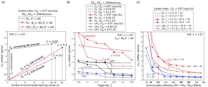
Figure 2: From left to right. (a) estimated carbon footprints of FL and CL for varying number of learning rounds: CL (black) is shown in dashed lines for $K=60$ devices, while FL (red with circle markers) and CFL (red with cross markers) are shown for $K=60$ devices and $K_{a}=40$ active ones on each round with $N=1$ neighbors; (b) estimated carbon emissions vs. target loss tradeoff ($K=60$, $K_{a}=40$, $N=1$) and varying CI: max EU (red), Italy (black) and Finland (blue); (c) estimated carbon emissions of CL, FL, and CFL for varying communication EE ranging from $50$ kbit/J to $400$ kbit/s, and networked devices: $K=30$ $(K_{a}=20)$, and $K=60$ ($K_{a}=40$). Optimal EE below which FL is more carbon efficient than CL is highlighted.

III Carbon footprint assessment

The carbon footprint evaluation assumes that each device $k$, including the server, is located in a specific geographical region characterized by a known carbon intensity ($\mathrm{CI}_{k}$) of electricity generation [15]. CI is measured in kg CO2-equivalent emissions per kWh (kgCO2-eq/kWh) which quantifies how much carbon emissions are produced per kilowatt hour of generated electricity. In the following, we consider the CI figures reported in EU back in 2019 [16]. Considering the energy models (1)-(3), carbon emission is evaluated by multiplying each individual energy contribution, namely $E_{k}^{(\mathrm{C})}$ and $E_{k,h}^{(\mathrm{T})}$ by the corresponding intensity values $\mathrm{CI}_{k}$. Carbon footprints and the proposed framework are summarized in Table II for CL ($C_{\mathrm{CL}}$) and FL policies ($C_{\mathrm{FL}}$) and ($C_{\mathrm{CFL}}$).

To analyze the main factors that impact the estimated carbon emissions, a few simplifications to the energy models (1)-(3) are introduced in the following. Communication and computing costs are quantified on average, in terms of the corresponding energy efficiencies (EE). Communication EE for DL ($\mathrm{EE}_{\mathrm{D}}=[E_{0,k}^{(\mathrm{T})}]^{-1}$), UL ($\mathrm{EE}_{\mathrm{U}}=[E_{k,0}^{(\mathrm{T})}]^{-1}$) and mesh networking ($\mathrm{EE}_{\mathrm{M}}=[E_{k,h}^{(\mathrm{T})}]^{-1}$) are measured in bit/Joule [bit/J] and describe how much energy is consumed per correctly received information bit [17]. Efficiencies depend on device/server consumption for communication $P_{\mathrm{T}}$ and net UL/DL or mesh throughput $R$. Depending on network implementations, we consider different choices of $\mathrm{EE}_{\mathrm{D}}$, $\mathrm{EE}_{\mathrm{U}}$ and $\mathrm{EE}_{\mathrm{M}}$. The computing efficiency, $\mathrm{EE}_{\mathrm{C}}=[E_{0}^{(\mathrm{C})}]^{-1}$, quantifies the number of rounds per Joule [round/J], namely how much energy per learning round is consumed at the data center (or PS). Devices equipped with embedded low-consumption CPUs typically experience a larger time span $T_{k}>T_{0}$ to process an individual batch of data; on the other hand, they use much lower power ($P_{k}$). Device computing $\mathrm{EE}$ is typically larger and modeled here as $\frac{\mathrm{EE_{\mathrm{C}}}}{\varphi}$ with $\varphi=E_{k}^{(\mathrm{C})}/E_{0}^{(\mathrm{C})}<1$. Typical values for communication and computing $\mathrm{EE}$ are in Table I.

In the proposed FL implementation, the set of $K_{a}$ active FL devices changes according to a round robin scheduling, other options are proposed in [19]. Considering typical CFL implementations, such as gossip [6], we let the devices choose up to $N=1$ neighbors per round. When ad-hoc mesh, or D2D, communication interfaces are not available, the energy cost to implement the generic peer-to-peer link ($k,h$) roughly corresponds to an UL transmission from the source $k$ to the core network access point (i.e., router), followed by a DL communication from the router(s) to the destination device $h$, namely $E_{k,h}^{(\mathrm{T})}\simeq E_{k,0}^{(\mathrm{T})}+E_{0,h}^{(\mathrm{T})}$, or equivalently $[\mathrm{EE}_{\mathrm{M}}]^{-1}\simeq[\mathrm{EE}_{\mathrm{D}}]^{-1}+[\mathrm{EE}_{\mathrm{U}}]^{-1}$. Router can be a host or base-station. In mesh networks, further optimization via power control [18] may be also possible depending on the node deployment. Since devices do not need the router to relay information to the PS, which may be located in a different country, substantial energy savings are expected.

TABLE III: Number of rounds (min-max), communication/computing energy costs and corresponding carbon footprints for selected cases, varying losses $\overline{\xi}$, and IID vs. non-IID data distributions. $\mathrm{EE}_{\mathrm{U}}=\mathrm{EE}_{\mathrm{D}}=100$ kbit/J

IV Industry 4.0 robotized environment

According to [20], in 2019 industry was responsible for about $30$% of the world greenhouse gas emissions. To counter this impact, Industry 4.0 (I4.0) and other mitigation policies have been recently introduced [21]. In line with the I4.0 paradigm, we resort to a common Industrial Internet of Things (IIoT) scenario where AI-based sensors and machines are interconnected and co-located in the same plant [22]. These sensors interact within an industrial workspace where human workers are co-present. Devices are served by a WiFi (IEEE 802.11ac) network and a router ($P_{\mathrm{T}}=6$ W [23]) is in charge of orchestrating the mesh communication or forwarding to the data center, or PS.

IV-A Case study: scenario-dependent setup

The goal of the training task is to learn a ML model for the detection (classification) of the position of the human operators sharing the workspace, namely the human-robot distance $d$ and the direction of arrival (DOA) $\theta$. Further details about the the robotic manipulators, the industrial environment and the deployed sensors are given in [2], [18]. Input data $\mathbf{x}_{h}$, available online [24], are range-azimuth maps obtained from $3$ time-division multiple-input-multiple output (TD-MIMO) frequency modulated continuous wave (FMCW) radars working in the $77$ GHz band [22]. During the on-line workflow, position ($d$, $\theta$) information are obtained from the trained ML model and sent to a programmable logic controller for robot safety control (e.g., emergency stop or replanning tasks). The ML model adopted for the classification of the operator location is a simplified version of the DeepMind [9]. It consists of $5$ trainable layers and $3$M parameters, of which $170$k are compressed, encoded by $16$ bits and exchanged during FL. Model outputs are reduced to $C=6$ for the detection of $6$ subject locations around the robot, detailed in [24]. Batch times and size of exchanged model parameters $b(\mathbf{W})$ (kB) are reported in Table I. Adam optimizer is used with a Huber loss [5]. The number of devices ($K$) is in the range $30\leq K\leq 60$, data can be identically distributed (IID) or non-IID. Moreover, $20\leq K_{a}\leq 40$ and $N=1$ are assumed.

Energy and carbon footprints are influenced by data center and device hardware configurations. The data center hardware consumption is reported in Table I and uses CPU (Intel i7 8700K, $3.7$ GHz, $64$ GB) and GPU (Nvidia Geforce GTX 1060, $1.5$ GHz, $3$ GB). For FL devices, we use Raspberry Pi 4 boards based on a low-power CPU (ARM-Cortex-A72 SoC type BCM2711, $1.5$ GHz, $8$ GB). These devices can be viewed as a realistic pool of FL learners embedded in various IIoT applications. FL is implemented using Tensorflow v$2.3$ backend (sample code available also in [24]). In what follows, rather than choosing a specific communication protocol, we follow a what-if analysis approach, and thus we quantify the estimated carbon emissions under the assumption of different DL/UL communication efficiencies ($\mathrm{EE}$). Since actual emissions may be larger than the estimated ones depending on the specific protocol overhead and implementation, we will highlight relative comparisons.

IV-B Case study: carbon footprint analysis

Fig. 2 provides an estimate of the carbon footprint under varying settings as detailed in Table I. Fig. 2(a) shows the carbon footprint for varying number of learning rounds ($n$), comparing CL with $K=60$ devices and FL with $K_{a}=40$. For CL (dashed line), an initial energy cost shall be paid for UL raw data transmission, which depends on the data size $b(\mathcal{E}_{k})$ and the communication EE; in this example, $\mathrm{EE}_{\mathrm{U}}=\mathrm{EE}_{\mathrm{D}}=200$ kbit/J. Next, the energy cost is only due to computing ($40$ J/round), unless new labelled data are produced by devices before the learning process ends on the data center. In contrast to CL, FL footprint depends on communication and computing energy costs per round. CFL (cross markers) has a cost of $224$ J/round, smaller than FL, namely $287$ J/round (circle markers) as PS is not required. Notice that mesh communication is replaced by UL and DL WiFi transmissions to/from a router.

Energy and accuracy loss $\xi$ can be traded off to optimize efficiency. For example, CL needs $n=25$ rounds at the data center to achieve a loss of $\xi=0.08$ and a carbon footprint of $2.9$ gCO2-eq. Model training should be typically repeated every $3$ hours to track modifications of the robotic cell layout, which corresponds to a total carbon emission of $8.4$ equivalent kgCO2-eq per year. CFL trains for more rounds (here $n=27$) to achieve a slightly larger loss ($\xi=0.2$), but reduces the emissions down to $1.7$ gCO2-eq, or $4.9$ kgCO2-eq per year, if training is repeated every $3$ hours. Finally, FL achieves a similar footprint, however this comes in exchange for a larger validation loss ($\xi=0.3$) due to communication with the PS. Although not considered here, tuning of model as well as changing the aggregation strategy at the PS [5] would reduce the training time and thus emissions.

The end-to-end energy cost is investigated in Figs. 2(b) and 2(c). Energy vs. loss trade-off is first analyzed in Fig. 2(b). We consider $3$ setups where the data center and the devices are placed in different geographical areas featuring different carbon indexes (CIs). In particular, the first scenario (max EU, red) is characterized by devices located in a region that produces considerable emissions as $\mathrm{CI}_{k}=0.97$ kgCO2-eq/kWh. This corresponds to the max emission rate in EU [16]. In the second (IT, black) and third (FI, blue) scenarios, devices and data center are located in Italy, $\mathrm{CI}_{k}=0.28$ kgCO2-eq/kWh, and Finland, $\mathrm{CI}_{k}=0.11$ kgCO2-eq/kWh, respectively. When the availability of green energy is small (i.e., max EU scenario, $\mathrm{CI}_{k}=0.97$), the learning loss and accuracy must be traded with carbon emissions. For example, for an amount of gas emission equal, or lower, than CL, the learning loss of CFL should be increased to $\overline{\xi}=0.1$, corresponding to an average accuracy of $90\%$. Considering FL, this should be increased to $\overline{\xi}=0.25$. For smaller carbon indexes, i.e. IT and FI scenarios, the cost per round reduces. Therefore, FL can train for all the required rounds and experience the same loss as in CL with considerable emission savings ($30\%\div 40\%$ for Finland). A promising roadmap for FL optimization is to let local learners contribute to the training process if, or when, green energy, namely small $\mathrm{CI}_{k}$, is made available.

In Fig. 2(c) we now quantify the carbon emissions of CL, FL and CFL for varying communication EE, ranging from $\mathrm{EE}_{\mathrm{U}}=\mathrm{EE}_{\mathrm{D}}=50$ kbit/J to $400$ kbit/J, and number of devices, $K=30$ $(K_{a}=20)$, and $K=60$ ($K_{a}=40$). An increase of the network size or a decrease of the network kb/J efficiency cause communication to emit much more CO2 than training. Since FL is more communication efficient as (compressed) model parameters are exchanged, in line with [3], the best operational condition of FL is under limited communication $\mathrm{EE}$ regimes. For the considered scenario, the optimal EE below which FL leaves a smaller carbon footprint than CL is in the range $50\%\div 100$ kbit/J for FL ($\overline{\xi}=0.2$) and $250\%\div 300$ kbit/J for CFL ($\overline{\xi}=0.1$). Finally, notice that for all cases FL can efficiently operate under $\mathrm{EE}=50$ kbit/J, typically observed in low power communications [25], and 4G/5G NB-IoT [26].

Table III compares the energy and carbon footprints for IID and non-IID data distributions. Computing, communication energy costs and corresponding carbon emissions for different target losses are evaluated with respect to the max EU scenario. Considering FL and CFL, federated computations are now distributed across $K_{a}$ devices, therefore larger computing costs are needed. Non-IID data generally penalizes both FL and CFL as energy consumption increases up to $40\%$ in some cases. For example, while CFL with IID data limits the number of required epochs (targeting $\overline{\xi}=0.1$) to a maximum of $n=43$, it is less effective for non-IID distributions as the required rounds now increase up to $n=62$ for some devices. CFL and FL thus experience an increase in energy costs, but CFL still emits lower carbon emissions. More advanced gradient-based CFL methods [7] might be considered when data distributions across devices are extremely unbalanced.

V Conclusions

This work developed a framework for the analysis of energy and carbon footprints in distributed and federated learning (FL). It provides, for the first time, a trade-off analysis between vanilla and consensus FL on local datasets, and centralized learning inside the data center. A simulation framework has been developed for the performance analysis over arbitrarily complex wireless network structures. Carbon equivalent emissions are quantified and discussed for a continual industrial workflow monitoring application that tracks the movements of workers inside human-robot shared workspaces. The ML model is periodically (re)trained to track changes in data distributions. In many cases, energy and accuracy should be traded to optimize FL energy efficiency. Furthermore, by eliminating the parameter server, as made possible by emerging decentralized FL architectures, further reducing the energy footprint is a viable solution. Novel opportunities for energy-aware optimizations are also highlighted. These will target the migration of on-device computations where the availability of green energy is larger. Finally, FL requires a frequent and intensive use of the communication interfaces. This mandates a co-design of the federation policy and the communication architecture, rooted in the novel 6G paradigms.

References

- [1] M. Dayarathna, et al., “Data Center Energy Consumption Modeling: A Survey,” IEEE Communications Surveys & Tutorials, vol. 18, no. 1, pp. 732-794, First quarter 2016.
- [2] S. Savazzi et al. “Opportunities of Federated Learning in Connected, Cooperative and Automated Industrial Systems,” IEEE Communications Magazine, vol. 52, no. 2, February 2021. [Online]. Available: https://arxiv.org/abs/2101.03367.
- [3] X. Qiu, et al.. “Can Federated Learning Save the Planet?” NeurIPS - Tackling Climate Change with Machine Learning, Dec. 2020, Vancouver, Canada. [Online]. Available: https://arxiv.org/abs/2010.06537
- [4] J. Konečný, et al. “Federated optimization: Distributed machine learning for on-device intelligence,” CoRR, 2016. [Online]. Available: http://arxiv.org/abs/ 1610.02527.
- [5] P. Kairouz, et al., “Advances and open problems in federated learning,” [Online]. Available: https://arxiv.org/abs/1912.04977.
- [6] M. Blot, et al., “Gossip training for deep learning,” 30th Conference on Neural Information Processing Systems (NIPS), Barcelona, Spain, 2016. [Online]. Available: https://arxiv.org/abs/1611.09726.
- [7] S. Savazzi, et al. “Federated Learning with Cooperating Devices: A Consensus Approach for Massive IoT Networks,” IEEE Internet of Things Journal, vol. 7, no. 5, pp. 4641-4654, May 2020.
- [8] Z. Chen, et al., “Consensus-Based Distributed Computation of Link-Based Network Metrics,” IEEE Signal Processing Letters, vol. 28, pp. 249-253, 2021.
- [9] V. Mnih, K. Kavukcuoglu, D. Silver, et al. “Human-level control through deep reinforcement learning,’ Nature 518, 529?533, 2015.
- [10] E. Masanet, et al., “Characteristics of low-carbon data centres,” Nature Climate Change, vol. 3, no. 7, pp. 627–630, 2013.
- [11] A. Capozzoli, et al. “Cooling systems in data centers: state of art and emerging technologies,” Energy Procedia, vol. 83, pp. 484–493, 2015.
- [12] H. Xing, et al., “Decentralized Federated Learning via SGD over Wireless D2D Networks,” Proc. IEEE 21st Int. Workshop on Signal Processing Advances in Wireless Comm. (SPAWC), Atlanta, GA, USA, pp. 1–5, 2020.
- [13] N. Shlezinger, et al. “Federated Learning with Quantization Constraints,” Proc. of IEEE International Conference on Acoustics, Speech and Signal Processing (ICASSP), Barcelona, Spain, pp. 8851–8855, 2020.
- [14] A. Elgabli, et al., “GADMM: Fast and Communication Efficient Framework for Distributed Machine Learning,” Journal of Machine Learning Research, vol. 21, no. 76, pp. 1–39, 2020.
- [15] L.F.W. Anthony, et al., “Carbontracker: Tracking and Predicting the Carbon Footprint of Training Deep Learning Models,” Proc of ICML Workshop on Challenges in Deploying and monitoring Machine Learning Systems, 2020.
- [16] European Environment Agency, Data and maps: “Greenhouse gas emission intensity of electricity generation,” Dec. 2020. [Online]. Available: https://tinyurl.com/36l5v5ht
- [17] E. Björnson and E. G. Larsson, “How Energy-Efficient Can a Wireless Communication System Become?,” Proc. 52nd Asilomar Conf. on Sig., Syst., and Comp., Pacific Grove, CA, USA, 2018, pp. 1252–1256.
- [18] S. Savazzi, et al. “A Joint Decentralized Federated Learning and Communications Framework for Industrial Networks,” Proc. of IEEE CAMAD, Pisa, Italy, pp. 1–7, 2020.
- [19] M. M. Amiri, et al., “Federated learning over wireless fading channels,” IEEE Trans. Wireless Commun., vol. 19, no. 5, pp. 3546–3557, May 2020.
- [20] J. G. J. Olivier, et al., “Trend in global CO2 and total greenhouse gas emissions,” 2020 Report, PBL Netherland Environmental Assessment Agency, Dec. 2020. [Online]. Available: https://tinyurl.com/xzz7btj6
- [21] H. Fekete, et al. “A review of successful climate change mitigation policies in major emitting economies and the potential of global replication,” Renewable and Sustainable Energy Reviews, vol. 137, art. 110602, 2021.
- [22] S. Kianoush, et al., “A Multisensory Edge-Cloud Platform for Opportunistic Radio Sensing in Cobot Environments,” IEEE Internet of Things Journal, vol. 8, no. 2, pp. 1154–1168, 2021.
- [23] The Power Consumption Database: WiFi routers. [Online]. Available: http://www.tpcdb.com/. Accessed: 08/03/2021.
- [24] Dataset: “Federated Learning: mmWave MIMO radar dataset for testing, ” IEEE Dataport, 2020. [Online]. Available: http://dx.doi.org/10.21227/0wmc-hq36 Accessed: March. 2021.
- [25] X. Vilajosana, et al., “IETF 6TiSCH: A Tutorial,” IEEE Communications Surveys & Tutorials, vol. 22, no. 1, pp. 595–615, Firstquarter 2020.
- [26] S. Zhang, et al., “Energy efficiency for NPUSCH in NB-IoT with guard band,” ZTE Commun., vol. 16, no. 4, pp. 46–51, Dec. 2018.