Probabilistic Forecasting of Regional Net-load with Conditional Extremes and Gridded NWP

Abstract

The increasing penetration of embedded renewables makes forecasting net-load, consumption less embedded generation, a significant and growing challenge. Here a framework for producing probabilistic forecasts of net-load is proposed with particular attention given to the tails of predictive distributions, which are required for managing risk associated with low-probability events. Only small volumes of data are available in the tails, by definition, so estimation of predictive models and forecast evaluation requires special attention. We propose a solution based on a best-in-class load forecasting methodology adapted for net-load, and model the tails of predictive distributions with the Generalised Pareto Distribution, allowing its parameters to vary smoothly as functions of covariates. The resulting forecasts are shown to be calibrated and sharper than those produced with unconditional tail distributions. In a use-case inspired evaluation exercise based on reserve setting, the conditional tails are shown to reduce the overall volume of reserve required to manage a given risk. Furthermore, they identify periods of high risk not captured by other methods. The proposed method therefore enables user to both reduce costs and avoid excess risk.

I Introduction

The nature of distribution networks is changing fundamentally as the penetration of generation, storage and flexible loads connected to them has grown over recent decades. Transmission networks are no longer simply supplying energy to meet the demand of connected consumers, but the net-load of consumption less production. Some distribution networks may even export energy to the transmission system during times of high renewable output. This complexity makes predicting future net-load far more challenging than conventional load forecasting, while such forecasts are increasingly valuable to both system operators and energy market participants. Furthermore, probabilistic forecasts have an important role to play in communicating forecast uncertainty which is impacted by the composition of net-load at any given time.

Our focus here is twofold: first, how to incorporate embedded generation in probabilistic load forecasts through use of weather forecasts and limited knowledge of installed capacities; and second, how to best describe the tails of predictive distributions which, while being valuable for many users, is challenging and has received little attention in the literature. While domestic solar is seen as the main challenge in some areas, in Great Britain and elsewhere small-scale wind, MW-scale solar arrays, batteries, and small thermal plant, such as waste-to-power plants and CHP, are often ‘embedded’ and only visible to network operators as negative load. In 2018, the last year of the case study presented in this paper, net-load on the Great Britain (GB) electricity transmission system (also called Transmission System Demand) ranged from 18GW to 50GW, with 13GW and 6GW of embedded solar and wind capacity, respectively, and a further 12GW of embedded conventional plant, mostly gas-fuelled. Periods of low load and high wind and solar generation present a significant challenge to the Transmission System Operator (TSO) due to their lack of visibility and control-ability of embedded generation [1].

There is a large literature on probabilistic load forecasting and such forecasts are increasingly being adopted by users in industry. Hong et al review the topic in [2] and highlight net-load forecasting as a new problem. Since then, day-ahead net-load forecasting at neighbourhood level has been studied in [3], but only deterministic predictions are considered. Probabilistic forecasts in the form of intervals are studied in [4] and [5] in the context of increasing embedded solar. While the former focuses on customer aggregation, the latter considers reserve scheduling and reaches the conclusion that greater reserves are required to manage increased uncertainty.

Regarding specific forecasting methodology, Hong et al conclude that that “a universally best technique simply does not exist”. Indeed, the implementation of prediction algorithms is of comparable importance to the choice of algorithm itself, with performance sensitive to hyper-parameter tuning, data preparation, and feature engineering, for example. That said, a high-level observation can be made that non-parametric probabilistic forecasting, and quantile regression in particular, is generally favoured [6, 7]. When considering net-load, it is reasonable to expect that innovations in wind and solar generation forecasting may enhance the accuracy of net-load forecasts. For instance, sky cameras has been used for 10–30 minute-ahead net-load forecasting with high penetrations of embedded solar [8]. Additionally, leveraging a grid of Numerical Weather Predictions (NWPs), rather than a single point, can improve day-ahead wind and solar forecasts markedly [9], a concept we adapt for net-load forecasting here, following the holistic variable selection approach of Xie and Hong [10].

For many users, the accuracy of extreme probabilities is an important aspect of probabilistic forecasting, i.e. the tails of predictive distributions. Quantile regression is widely used for probabilistic forecasting as it makes no assumptions about the shape of predictive distributions, but is not well suited to estimating conditional extremes as data is increasingly sparse in the tails, so special treatment is required. While there are well established practices modelling extreme events for planning purposes [11], such heat waves, the extremes of short-term forecast errors and uncertainty have received little attention. Panteli et al discuss the importance of short-term forecasts of extremes in power system resilience in [12] and highlighted this as an area where development of advanced tools is required. It should be noted that severe weather events are typically well forecast in the short-term, and that extremes of short-term forecast errors/uncertainty do not necessarily correspond to extreme weather.

Extreme value theory provides a theoretical framework for this task, particularly the peaks-over-threshold method and the resulting Generalised Pareto Distribution (GPD) [13]. The GPD has recently been applied to the tails of probabilistic wind power forecasts and shown to be effective where quantile regression fails [14]. We propose applying a similar technique for net-load here, but, while in [14] the GPD parameters are fixed, we allow them to depend on covariates along the lines of [15]. In the case of net-load, we suspect that, similarly to the central portion of the predictive distribution, the tails will depend on behavioural and weather effects. In the remainder of this paper we use ‘extreme’ refer to probability levels where standard quantile regression is not suitable.

Energy forecasts of varying levels of sophistication play an important role in reserve setting and procurement, a process that impacts the cost of operating a power system and its reliability [16, 17, 18]. Requirements for reserve services are set to meet a given risk appetite based on the probability of events such as unplanned plant outages and large forecast errors. In a risk-neutral setting, the relevant probability is the ratio of the marginal reserve cost to value of lost load, typically 0.01%–0.25%, which is approximately the same range bounded by common heuristics 1 hour and 1 day-per-year. Forecasts of net-load are therefore required at these probability levels. The impact of solar penetration on net-load and reserve setting was recently explored in [5] concluding that the need for reserve increases with solar penetration based on 95% prediction interval width. Here, we develop a similar approach to quantify the value of forecast improvement in terms of volume of reserve required to manage forecast uncertainty and compare regions with differing types and capacities of embedded generation.

This paper contributes a novel model structure for probabilistic net-load forecasts in the presence of embedded wind and solar generation, including a methodology for forecasting extreme quantiles; an evaluation framework for the tails of predictive distributions previously lacking; and the augmentation of net-load forecasts using features derived from gridded NWP data. These methods are demonstrated on large dataset which is published along with the paper, and their performance is evaluated in terms of both statistical metrics and practical value for procuring reserve services.

II Net-load Forecasting

Electricity load forecasting has been the focus of much research resulting in a range of models which may be considered ‘best-in-class’ for this task [2]. For the purposes of exploring the value of gridded NWP and estimation of extreme quantiles, we have selected one such approach for producing probabilistic forecasts of non-extreme quantiles, that of [19] based on Generalised Additive Models (GAMs) and linear quantile regression, which won the load track of GEFcom2014. We also consider Tao’s Vanilla Benchmark as an additional reference model [20], extended using linear quantile regression in the same way as the aforementioned GAMs.

II-A Generalised Additive Models for Location Shape and Scale

TABLE I: Description of forecasting models and feature sets used by each. Feature sets are detailed in Table II.

Model	Description
Vanilla-T	Tao’s Vanilla Benchmark [20]
GAM-T	GAM with date/time and temperature features only
Vanilla-Point	Tao’s Vanilla Benchmark with addition of linear wind speed and solar irradiance features
GAM-Point	GAM-T with additional standard NWP features
GAM-Grid	GAM-Point with additional features derived from gridded NWP

Let $y_{t}$ be the net-load at time $t$ and indicate with $F_{t}(y_{t})$ its cumulative probability distribution. In a distributional regression context, $F_{t}(y_{t})$ is modelled via a parametric model, $F(y_{t}|\bm{\theta}_{t})$, where $\bm{\theta}_{t}$ is an $m$-dimensional vector of parameters. In Generalised Additive Model for Location, Scale and Shape (GAMLSS) [21] the elements $j=1,...,m$ of $\bm{\theta}_{t}$ are modelled via

$$g_{j}(\theta_{j,t})=\mathbf{A}_{j,t}\bm{\beta}_{j}+\sum_{i}f_{j,i}({\bm{x}}^{S_{j,i}}_{t}),\;\;\;\text{for}\;\;\;j=1,\dots,m,$$ (1)

where $g_{j}$ is a monotonic function, $\mathbf{A}_{j,t}$ is the $t$-th row of the design matrix $\mathbf{A}_{j}$, $\bm{\beta}_{j}$ is a vector of regression coefficients, $\bm{x}_{t}$ is a $d$-dimensional vector of covariates and $S_{j,i}\subset\{1,\dots,d\}$. Hence, if $S_{j,i}=\{1,3\}$, then following our notation ${\bm{x}}_{t}^{S_{j,i}}$ is a two dimensional vector formed by the first and third element of $\bm{x}_{t}$. Each $f_{j,i}$ is a smooth function, built via

$$f_{j,i}(\bm{x}^{S_{j,i}})=\sum_{k=1}^{K_{j,i}}b^{ji}_{k}(\bm{x}^{S_{j,i}})\beta_{k}^{ji},$$ (2)

where $b^{ji}_{k}$ are spline basis functions of dimension $|S_{j,i}|$, while $\beta_{k}^{ji}$ are regression coefficients. The smoothness of each $f_{j,i}$ is controlled via ridge penalties, the definition of smoothness being dependent on the type of effect and penalty being used. In this work we will use the term generalised additive model (GAM) to indicate a restricted GAMLSS model where only one element of $\bm{\theta}_{t}$ is modelled as in (1), while the other elements are kept constant. See [22] for a detailed introduction to GAM/GAMLSS models, smoothing splines bases and penalties.

II-B Multiple Quantile Regression

Quantile regression enables the construction of a non-parametric predictive distribution by from multiple conditional quantiles. While [23] provides method for fitting quantile GAMs, these are too computationally demanding for the forecasting application considered here, which requires many complex model fits. Therefore, we apply linear quantile regression to the residuals of the main GAM (or Vanilla) model with a reduced feature set, $\mathbf{B}_{t}$. The predictive quantile for probability level $\alpha$ is given by

$$q_{\alpha,t} = \hat{y}_{t}+\mathbf{B}_{t}\beta_{\alpha}\quad,$$ (3)

where $\hat{y}_{t}$ is the deterministic forecast, which is an estimate of the conditional expectation produced by a Gaussian GAM (or Vanilla model) and $\beta_{\alpha}$ are model parameters to be estimated. The features $\mathbf{B}_{t}$ may be either exogenous variables or, following [19], the design matrix of linear terms from the fitted GAM model.

The predictive distribution $\hat{F}_{\text{QR},t}(y_{t})$ is constructed by estimating multiple quantiles at a range of probability levels $\alpha_{L},...,\alpha_{R}$ and interpolating between them to produce a continuous cumulative distribution function. An obvious drawback of this approach is that the predictive distribution is not defined for probabilities below $\alpha_{L}$ or above $\alpha_{R}$. For some applications this may be of no consequence, but where full support is required, such as sampling, modelling dependency using copulas, or setting reserves based on extreme quantiles, a solution is needed. One simple solution is to confine distribution within a upper and lower boundaries by assigning values to $q_{0,t}$ and $q_{1,t}$ and including them in the interpolation scheme. If the target variable is bounded by physical or other known restrictions, then this may be justified provided that $\alpha_{L}$ is close enough to 0 (and $\alpha_{R}$ to 1) for the resulting interpolation to result in a distribution of reasonable quality. The alternative is to specify a parametric function describing the tails of the predictive distribution, and this is the subject of Section III.

II-C Weather and Date/time Features

Conventional load forecasting typically considers the impact of temperature on electricity consumption, which is largely heating and cooling demand, and also influenced to a lesser extent by wind chill, precipitation, and illumination. Furthermore, a single-valued weather feature is typically assumed to be representative for the geographic region of interest. This may be derived from one or more weather forecast/measurement locations, typically meteorological stations close to population centres, and/or multiple variables, as in the case of so-called composite weather variables.

In order to explore the value of weather features targeting embedded wind and solar generation, and more sophisticated treatment of weather data in general, we compare GAM models with the same basic structure but with different sets of weather features. NWPs are produced on a regular spatial grid and therefore contain information beyond ‘average’ conditions for given region. Statistics derived from gridded NWP such as spatial standard deviation, min, max and so on, encode potentially valuable information for predicting net-load in a region, as demonstrated for wind and solar production in [24], so we consider including them here in net-load forecasting models.

We consider a progression of models with increasingly sophisticated weather features combining best-practice from load and generation forecasting: We first consider models that only include calendar and point temperature features (labeled ‘-T’). Point temperatures forecasts are those for the single NWP cell corresponding to highest population density in a region. Next, we add the spatially-averaged wind speed and solar irradiance forecasts for each region combined with embedded wind and solar capacity, which may change significantly over time (labeled ‘-Point’). Finally, we include statistics such as spatial standard deviation, min and max derived from gridded NWP (labeled ‘-Grid’). Full lists of models and features are provided in Tables I and II, respectively.

Date/time features play a central role in load forecasting to capture diurnal, weekly and annual seasonality. Here we use the GAM framework to estimate a smooth time-of-day profile for nine day-types: each day of the week, public holidays and school holidays following [25]. We also include interactions between time-of-day and weather effects as these are known to elicit a different response depending on the time of day [20]. Autoregressive terms are also a common feature of short-term load forecasting and can capture diurnal and weekly seasonality as well as level-changes in load. However, we found them to be detrimental here, possibly due to the impact of embedded generation polluting the seasonal cycles, and instead opted to include a two-week rolling mean of net-load to capture level-changes with less sensitivity to individual lagged observations.

TABLE II: List of explanatory variables, type (L=linear, D=dummy, P($n$)=polynomial of order $n$, S=smooth, BS=bivariate smooth), and details of the cubic spline basis dimension $K$ used in GAM modelling. Features labeled $\checkmark_{q}$ are also as linear features in quantile regression, $\mathbf{B}_{t}$ in Equation (3). Calculation of weather features is described in Section II-C.

Terms	Type	Vanilla-T	GAM-T	Vanilla-Point	GAM-Point	GAM-Grid
Linear trend (time since 2014-01-01)	L	$\checkmark$		$\checkmark$
Clock-time (local time zone)	D	$\checkmark_{q}$		$\checkmark_{q}$
Day-type {Mon,Tue,…,Sun, Public Holiday}	D	$\checkmark_{q}$	$\checkmark_{q}$	$\checkmark_{q}$	$\checkmark_{q}$	$\checkmark_{q}$
Trend	P($2$)		$\checkmark$		$\checkmark$	$\checkmark$
Two-week rolling average net-load	L		$\checkmark$		$\checkmark$	$\checkmark$
Second-order Fourier (annual)	L		$\checkmark$		$\checkmark$	$\checkmark$
School Holiday (region-specific)	D		$\checkmark$		$\checkmark$	$\checkmark$
Clock-time (decimal hour in local time zone)	S, $K$=35		$\checkmark$		$\checkmark$	$\checkmark$
Clock-time by day-type	S, $K$=30		$\checkmark$		$\checkmark$	$\checkmark$
Clock-time by school holiday	S, $K$=20		$\checkmark$		$\checkmark$	$\checkmark$
Point temperature	P($3$)	$\checkmark_{q}$		$\checkmark_{q}$
Point temperature by clock-time	P($3$)	$\checkmark$		$\checkmark$
Point temperature by month	P($3$)	$\checkmark$		$\checkmark$
Point temperature	S, $K$=35		$\checkmark$		$\checkmark$	$\checkmark$
48-hour rolling mean point temperature	S, $K$=35		$\checkmark$		$\checkmark$	$\checkmark$
Population-weighted temperature	S, $K$=35					$\checkmark_{q}$
48-hour rolling mean population-weighted temperature	S, $K$=35					$\checkmark$
Population-weighted temperature and clock-time	BS, $K$=17					$\checkmark$
Mean irradiance scaled by solar capacity	L			$\checkmark_{q}$
Mean irradiance scaled by solar capacity	S, $K$=5				$\checkmark$	$\checkmark$
Mean irradiance and 10m wind speed	BS, $K$=17				$\checkmark$	$\checkmark$
Max irradiance scaled by solar capacity	S, $K$=5					$\checkmark$
Standard deviation of irradiance scaled by solar capacity	S, $K$=5					$\checkmark_{q}$
Max cloud cover scaled by solar capacity	S, $K$=5					$\checkmark$
Mean 10m wind speed	L				$\checkmark$	$\checkmark$
Mean 100m wind speed	L			$\checkmark_{q}$
Mean 100m wind speed by embedded wind capacity	S, $K$=20				$\checkmark_{q}$	$\checkmark_{q}$
Standard deviation of 100m wind speed	L					$\checkmark_{q}$
Day-ahead electricity price (N2EX) and clock-time	BS, $K$=17				$\checkmark$	$\checkmark$
Mean precipitation	S, $K$=5				$\checkmark$	$\checkmark$
Mean precipitation and clock-time	BS, $K$=17				$\checkmark$	$\checkmark$
Standard deviation of precipitation	S, $K$=5					$\checkmark$

III Conditional Extremes

Quantile regression is not well suited to estimating extreme conditional quantiles due to the sparsity of data by definition, which is further exacerbated by conditioning on exogenous variables [26]. The peaks-over-threshold method provides a parametric estimator for extreme quantiles, namely the scaled GPD, given by

$$F_{\text{GPD}}(y|\sigma,\xi)=\begin{cases}1-\left(1+\frac{\xi y}{\sigma}\right)^{-1/\xi}&\text{for }\xi\neq 0,\\ 1-\exp\left(-\frac{y}{\sigma}\right)&\text{for }\xi=0,\end{cases}$$ (4)

where the support of $Y$ is $y\geqslant 0$ when $\xi\geqslant 0\,$, and $0\leqslant y\leqslant-\sigma/\xi$ when $\xi<0$ [13]. The parameters of the GPD can be allowed to vary with the covariates as described in Section II-A, thus leading to the following GAMLSS model

$$g_{1}(\sigma_{t}) = \mathbf{C}_{1,t}\bm{\beta}_{1}+\sum_{i}f_{1,i}(x_{i,t})+...$$ (5)

$$g_{2}(\xi_{t}) = \mathbf{C}_{2,t}\bm{\beta}_{2}+\sum_{i}f_{2,i}(x_{i,t})+...$$ (6)

which may be estimated using the general GAM methods of [27].

Integrating the GPD model with quantile regression provides full support for $\hat{F}$, which now comprises conditional quantiles between probability levels $\alpha_{L}$ and $\alpha_{R}$, and two GPDs for probabilities $\alpha<\alpha_{L}$ and $\alpha>\alpha_{R}$. The predictive distribution $\hat{F}(y|\bm{x})$ may be written

$$\begin{cases}\alpha_{L}F_{\text{GPD}}(q_{\alpha_{L}}-y|\sigma_{L}({\bm{x}}),\xi_{L}({\bm{x}}))\hfill~{}\text{for }y<q_{\alpha_{L}},\\ \hat{F}_{\text{QR}}(y|{\bm{x}})\hfill~{}\text{for }q_{\alpha_{L}}\leq y\leq q_{\alpha_{R}},\\ \alpha_{R}+(1-\alpha_{R})F_{\text{GPD}}(q_{\alpha_{R}}+y|\sigma_{R}({\bm{x}}),\xi_{R}({\bm{x}}))\hfill~{}\text{for }y>q_{\alpha_{R}},\end{cases}$$ (7)

and illustrated in Figure 1.

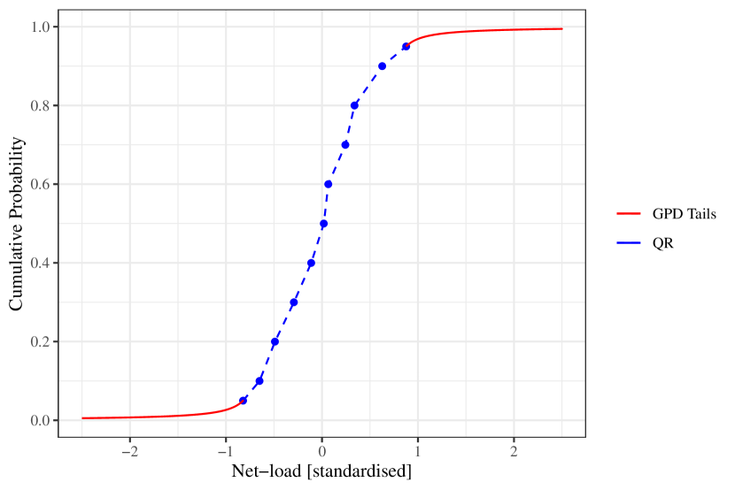
Figure 1: Illustration of predictive distribution comprising quantile regression (QR) between $\alpha_{L}=0.05$ and $\alpha_{R}=0.95$ and GPD tails described in Equation (7).

The choice of $\alpha_{L}$ and $\alpha_{R}$, which specify the points at which quantile regression meets the parametric tails, requires some consideration and depends on both data volume and complexity of the models involved (e.g. number of covariates). We suggest that quantile regression should be extended as far into the tail as possible, i.e. until $q_{\alpha_{L}}$ and $q_{\alpha_{R}}$ become unreliable or it becomes difficult to verify their reliability, based on a cross-validation exercise. This is the procedure we employ in the case study presented in Section V, but alternative strategies may be imagined.

In the context of net-load forecasting, we hypothesise that the tails of the predictive distribution depend on multiple factors, including time-of-day and weather effects (wind, solar, temperature), just as other conditional quantiles do. We therefore propose a model that allows the parameters of the tail distribution to depend on features that capture these effects.

We adopt a GAMLSS GPD model where the scale parameter is modelled via the link function $g_{1}(\cdot)=\log(\cdot)$, with linear effects for 100m wind speed and surface solar irradiation, and a smooth effect for the estimated expected net-load, built using four basis functions. The shape parameter $\xi$ is constant.

IV Evaluation Framework

This section introduces the methods and metrics we employ to evaluate and compare forecast performance. The objective of density forecasts it to be as sharp as possible while remaining reliable/calibrated [28]. A sharp forecast is synonymous with low uncertainty and is therefore of more value to decision makers. In addition to evaluating forecast based on this principle of ‘sharpness subject to calibration’, we consider the impact on a key use-case for net-load forecasting in Section V-C, namely reserve setting.

IV-A Pinball and Sharpness

The Pinball Score for an individual quantile matches the loss function minimised in quantile regression model estimation. The Pinball Score is given by

$$\frac{1}{T|\mathcal{A}|}\sum_{\alpha\in\mathcal{A}}\sum_{t=1}^{T}\left(q_{\alpha,t}-y_{t}\right)\left(\mathbb{1}(y_{t}\leq_{\alpha,t})-\alpha\right)$$ (8)

where $\mathcal{A}$ is the set of quantiles being estimated. A drawback of the Pinball Score is that it places greater weight on the performance of quantiles close to $\alpha=0.5$ and less on those in the tails of predictive distributions. While Pinball Scores for individual tail quantiles may be calculated, they suffer from high variance due to the sparsity of observations and are therefore not suitable for discriminating between different forecasting systems. Therefore, we also evaluate interval width, the average of the $(1-2\lambda)\%$ prediction interval $q_{1-\lambda,t}-q_{\lambda,t}$. In both cases, however, calibration must be verified separately.

IV-B Calibration

Calibration, also called ‘reliability’, is the property that forecast probabilities match the observed frequency of realisations. For example, if a forecast is calibrated, then 10% of observations should fall below the $\alpha=0.1$ predictive quantile, with some tolerance based on the finite number of available forecast-observation pairs. This property is necessary for forecast probabilities to be used in quantitative decision making. Calibration is typically evaluated visually using reliability diagrams, which plot the nominal coverage, $\alpha$, against observer frequency mean($\mathbb{1}(y_{t}\leq q_{\alpha,t})$).

Here we also examine so-called worm plots, a variant of the more familiar Q-Q plot, because they accentuate tail behaviours, which are of particular interest in this study [29]. We calculate consistency intervals considering the temporal correlation of net-load, as the usual assumption of independence between samples does not hold: if the data lies within the consistency interval then the forecast is consistent with being calibrated [30].

V Case Study

The proposed and benchmark methodologies described above are tested on a large dataset from GB which is attached to this article as supplementary material [31]. We define net-load as the load on the transmission system measured at the interface between transmission and distribution networks. In GB these interfaces are called Grid Supply Points, and are grouped into 14 regions called Grid Supply Point Groups (GSP Groups). Net-load is metered at half-hourly resolution and our dataset spans five years 2014–2018. Over this period the installed capacity of embedded solar in GB grew from 3GW to 13GW, presenting a particular challenge.

Historic weather forecasts from the operational ECMWF-HRES model are used. We use forecasts with a base time of 0000h UTC which become available at approximately 0600h UTC and are therefore suitable for day-ahead forecasting tasks where a new forecast is issued in the morning of day $D$ for all of $D+1$. Forecasts of wind speed at 10m and 100m, surface temperature, cloud cover, solar irradiation and total precipitation are extracted on a $0.1^{\circ}$ spatial grid and pre-processed as described in Section II-C. The spatial extent of each GSP Group is provided by National Grid ESO [32] and population density by the Office for National Statistics [33, 34]. We also include estimates of national embedded wind capacity from [32], estimates of regional solar capacity from [35], and public and school holidays.

Regions vary in size from maximum net-load of 6.3GW in Group A (East England) to 0.5GW in Group P (North Scotland), and minimum net-load of 1.9GW in Group C (Greater London) to significant export of -1.2GW in Group P. Prior to modelling and forecasting, all net-load data are standardised (converted to z-scores). A representative selection of results are presented here are in terms of standardised data for comparison between regions, in particular we highlight Groups C (city region), H (high solar) and P (high wind). Summary statistics of the dataset, the data itself and full results for all models and GSP Groups are available in [31].

Model development was carried out using three-fold cross-validation on data from 2014–2017 and final testing was performed on data from 2018. During the test phase GAMs were re-trained every two weeks in an expanding window fashion.

V-A Non-extreme Quantities

The central quantiles, $\alpha=0.1,0.2,...,0.9$, are evaluated to verify their calibration and compare performance in terms of the Pinball Score. The evaluation of reliability of the Vanilla-Point and GAM-Point models for all 14 GSP Groups is show in Figure 2. Both models have near perfect calibration of the cross-validation exercises (shown in [31]), which degrades a little for GAM-Point on the final test dataset but considerably more for Vanilla-Point. In the case of the latter’s forecasts, approximately half of the GSP Groups are clearly not calibrated, highlighting the value of the more flexible GAM modelling approach. This is the pattern for all GAM- and Vanilla- models (shown in [31]).

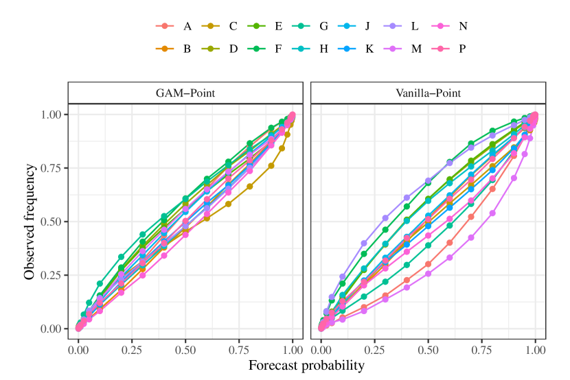
Figure 2: Reliability diagrams for GAM-Point and Vanilla-Point models and all GSP Groups on the Test set. If forecasts are calibrated the observed frequency of realisations falling below a given quantile $q_{\alpha}$ should match that quantile’s forecast probability $\alpha$.

The Pinball Score for all models and GSP Groups reveals similarly that the GAM approach results in superior forecasts compared to the Vanilla benchmarks, shown in Figure 3 and Table III. Furthermore, the importance of weather features related to embedded wind and solar generation are clear: Vanilla-T and GAM-T, the models with date/time and temperature features only, have extremely poor performance relative to their equivalents with additional wind and irradiance features. Comparing GAM-T and GAM-Point, the inclusion of additional weather forecast data results in a reduction of the Pinball Score by 40% overall, and the effect is more prominent the greater the capacity of embedded generation. For example the improvement is only 10% for Group C, the Greater London city region where there is little embedded generation but 60% for Group P, where the embedded wind capacity exceeds peak load. A small improvement from addition of features derived from gridded NWP is suggested by the cross-validation exercise but is not consistently reproduced on test data and therefore inconclusive (Not shown, see supplementary material for details [31]).

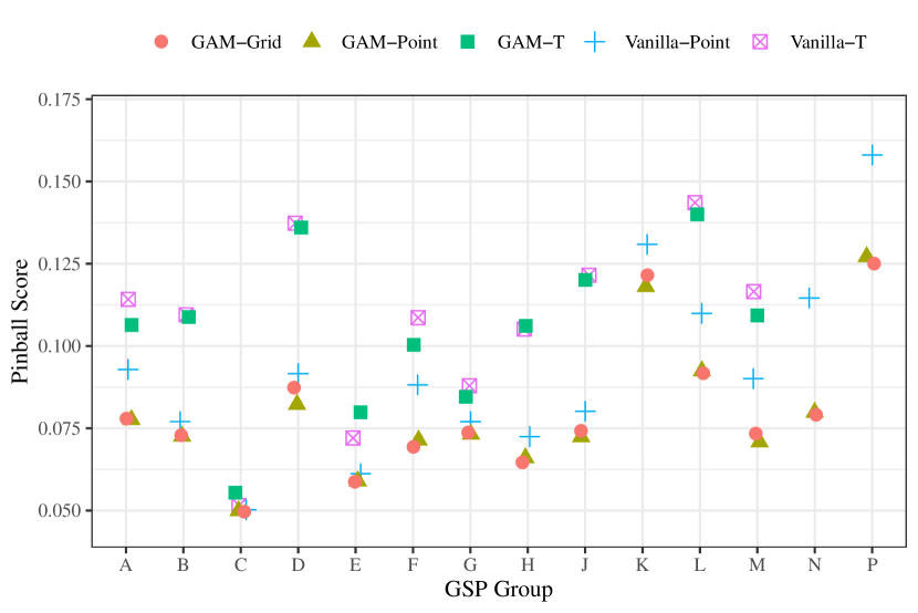
Figure 3: Pinball Score for each of the 14 GSP Groups form the cross-validation exercises averaged across quantiles $\mathcal{A}=\{0.1,0.2,...,0.9\}$. The score is calculated on standardised data so is unitless and comparable between regions of different size. Scores for GAM-T and Vanilla-T exceed 0.2 at GSP Groups K, N and P are not shown.

TABLE III: Pinball scores for cross-validation (CV) and Test exercises averages across all GSP Groups (All), and for Groups C, H and P. The score for the best performing model(s) in each case are emboldened. Where the difference between scores of the two best methods is not significant at the $p<0.05$ level both are emboldened or italicised.

	CV	Test
GSP Group	All	All	C	H	P
Vanilla-T	0.121	0.137	0.052	0.105	0.334
Vanilla-Point	0.083	0.092	0.050	0.072	0.158
GAM-T	0.120	0.134	0.055	0.106	0.324
GAM-Point	0.070	0.079	0.050	0.066	0.127
GAM-Grid	0.070	0.080	0.050	0.065	0.125

The significance of apparent differences in skill is examined using the Diebold-Mariano (DM) test [36]. For each GSP Group and pair of models we have calculated the Pinball Skill Score and associated $p$-value from the DM test. The result for average performance across all GSP Groups is shown in Figure 4. The $>10\%$ improvement of GAM-Point/-Grid over the Vanilla-Point benchmark is significant ($p<0.001$), and this is consistent across all GSP Groups. However, the skill of GAM-Grid relative to GAM-Point is more complex. Skill is positive and significant for GSP Groups F and H, significant and negative for Groups D, J and K, and not significantly different at GSP Groups the remaining nine (shown in [31]).

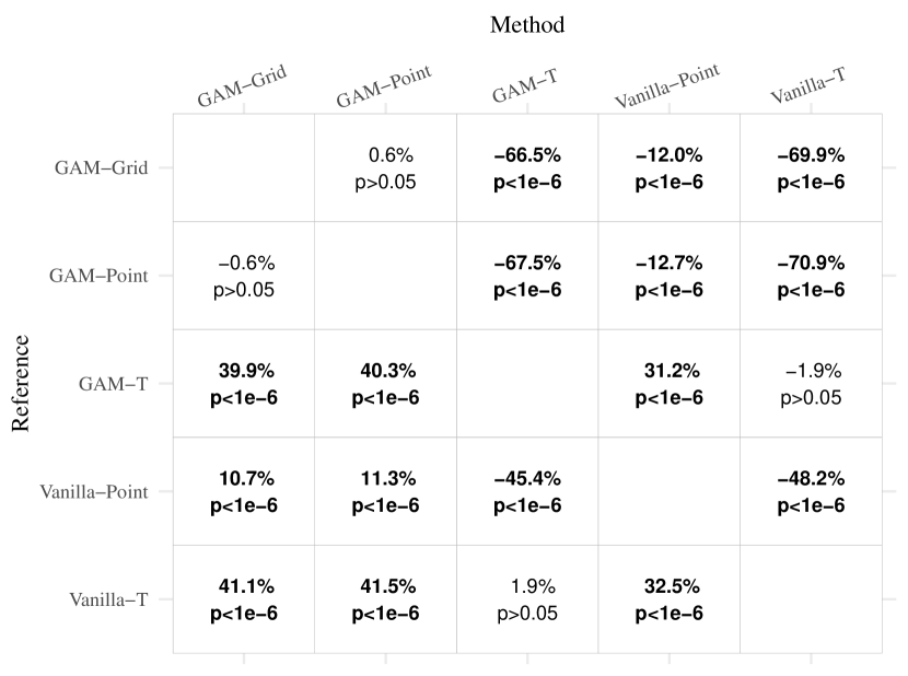
Figure 4: Pinball skill scores and significance ($p$-values from the Diebold-Mariano test [36]) for the all pairs of methods, computed on the test set. A value of $p<0.05$ indicates strong evidence that the skill of forecast produced by ‘Method’ relative to ‘Reference’ is not zero. These value are emboldened.

V-B Extreme Quantities

Extreme quantiles have been estimated using quantile regression in the same fashion as non-extreme quantiles for probability levels 0.05, 0.025, 0.01, 0.005, 0.0025, 0.001 and 0.0005, (and equivalent for right tail). Evaluation of their reliability in the cross-validation exercise identified the $\alpha_{L}=0.025$ and $\alpha_{R}=0.975$ (0.05 and 0.95, respectively, for GSP Groups E, F, L and P) as the last reliable quantiles in the present case study, so these are the probability levels beyond which GPD tails are used as an alternative approach to estimating extreme quantiles. We consider both a static GPD with constant parameters, and a conditional GPD (GAMLSS-type) where the scale parameter is a function of covariates and the shape parameter is constant, described in Section III.

The worm plots in Figure 5 evaluate the calibration of the predictive distributions, specifically the forecasts may be said to be ‘consistent with calibration’ if the lines are within the consistency intervals. This reveals that below 1% and above 99% the forecasts based on quantile regression only are not calibrated at any GSP Group. Therefore, these quantiles are not suitable for use in decision-making. However, those based on a combination of quantile regression and GPD tails are consistent with calibration.

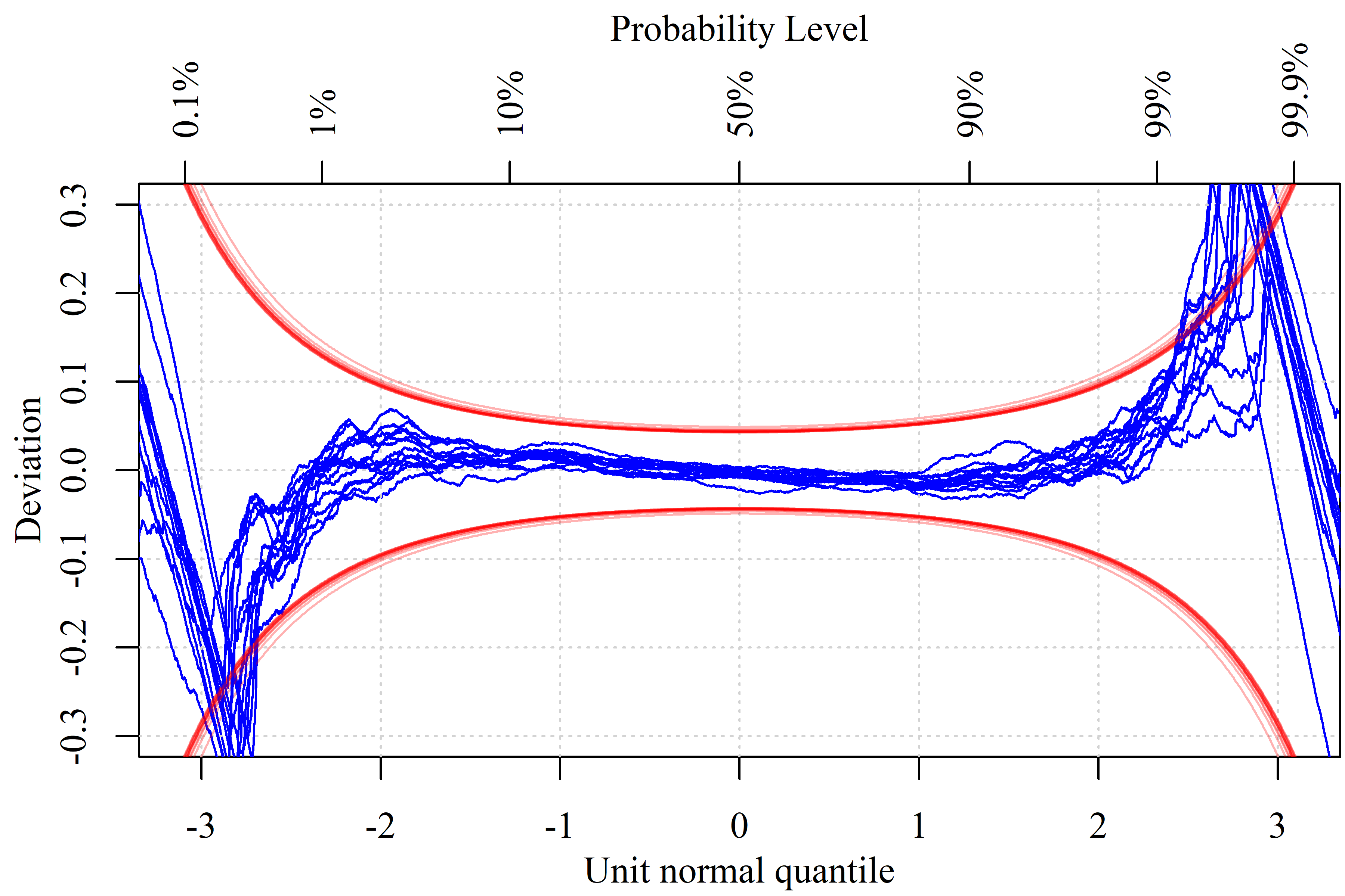
(a) Quantile Regression

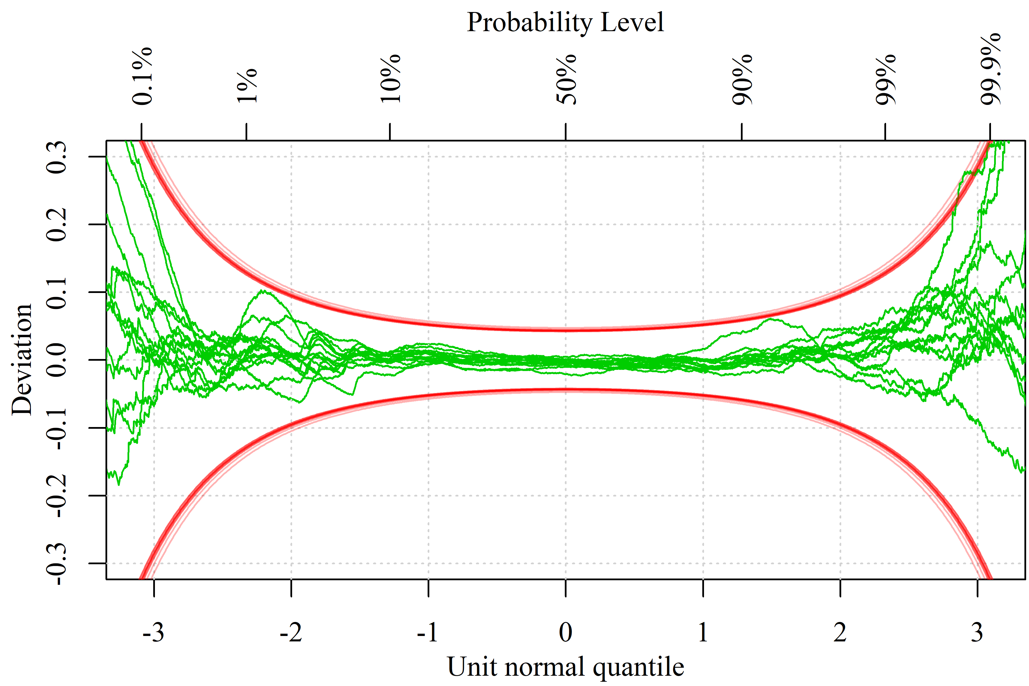
(b) Static GPD

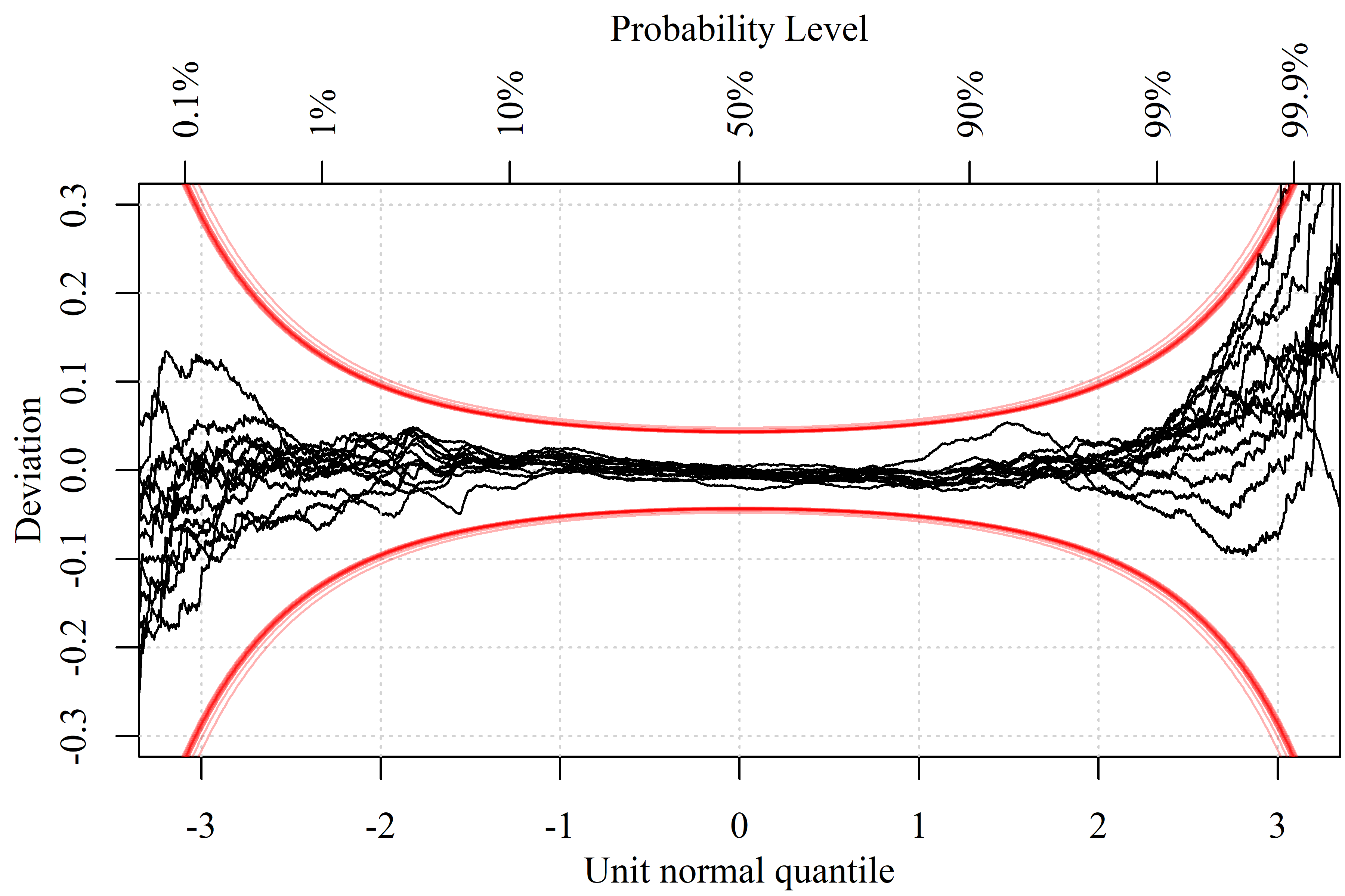
(c) Conditional GPD

Figure 5: Worm plots for GAM-Grid forecasts for 14 GSP Groups with quantile regression tails (left), static (centre) and conditional GPD tails (right). Consistency intervals are calculated for each GSP Group at the 95% level considering first-order auto-correlation and are overlaid in red. Forecasts that breach the consistency intervals are not consistent with being calibrated and therefore not suitable for use.

We have seen that both static and conditional GPD approaches produce calibrated forecasts, and are now interested in whether the relative complexity of the conditional models produce sharper forecasts. Average interval width is a simple measure of sharpness and visualised in Figure 6 for GAM-Grid forecasts with quantile regression, static GPD and conditional GPD tails for GSP Groups C, H and P. The 99.5%–99.9% interval forecasts using the conditional GPD are much sharper than those from the static version, with more pronounced difference at higher probabilities. The conditional GPD is therefore proving more confident forecasts than the static version, on average, while remaining calibrated. The practical value of this improvement is investigated in the next section. The intervals produced by quantile regression are sharper still, but as we have seen are not calibrated and therefore not usable.

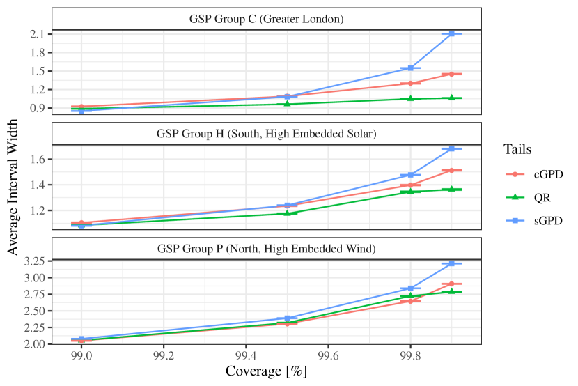
Figure 6: Sharpness diagrams for the GAM-Grid model with different approaches for estimating extreme quantiles. While quantile regression (QR) produces sharper intervals they are not calibrated so cannot be used. Of the two parametric approaches, which are calibrated, the conditional GPD (cGPD) produces sharper intervals than the static (sGPD). Bars are 95% confidence intervals calculated via bootstrap re-sampling. They illustrate sampling variation and verify the significance of differences in interval width.

V-C Use-case Evaluation: Reserve

Reserve is procured as a contingency to correct potential energy imbalances and the illustrative example here is based on current practice in GB. The amount to procure is chosen to satisfy the TSO’s risk appetite, e.g. reserve will be sufficient in all but 4 hours-per-year, which corresponds to the $\alpha=0.0005$ quantile of net-load for upwards reserve (and $\alpha=0.9995$ for downward). In this case we would calculate the upward reserve requirement in each 30-minute period to be $q_{0.5}-q_{0.0005}$ on the basis that the power system is scheduled according to the median forecast $q_{0.5}$.

In order to understand the impact of forecast performance on this task, we compare the volumes of reserve that would be procured using different forecasts. As well as total volumes, we are also concerned with the times of day when one forecast suggests procuring additional reserve because uncertainty is deemed high, compared to an alternative which is unable to discriminate between periods relatively high or low uncertainty. Furthermore, as an additional benchmark we consider the naive approach of procuring reserve volumes using the empirical quantiles of historic deterministic forecast errors rather than a specific probabilistic forecast. This approach implicitly assumes that forecast uncertainty is constant, but it is easy to interpret and similar to the heuristics based on ex-post analysis widely used in practice.

The practical benefits of the performance gain offered by forecasts with the conditional over static GPD tails discussed above translates into reduced volumes of both upwards and downward reserve. The former is reduced by up to 24.6% and the latter by up to 10.8% for probability levels 0.01%–0.25%, with greater impact at more extreme quantiles, see Table IV. The improvement is much greater when compared to the naive approach, especially at less extreme probability levels where the naive approach is particularly conservative.

TABLE IV: Percentage change in reserve volumes, and proportion of Periods (30 minute settlement periods) with lower reserve volumes, for forecasts based on conditional GPD tails relative to the naive and static GPD forecasts.

		cGPD vs Naive $[\%]$		cGPD vs sGPD $[\%]$
Reserve	Quantile	Volume	Periods	Volume	Periods
Upward	0.01%	-18.0	77.0	-24.6	81.3
	0.05%	-16.5	73.6	-13.9	70.4
	0.1%	-17.2	74.1	-9.1	63.3
	0.25%	-16.5	71.8	-3.2	55.9
Downward	99.75%	-19.8	81.4	-0.8	59.7
	99.9%	-22.1	84.0	-3.2	64.1
	99.95%	-22.9	84.7	-5.3	67.3
	99.99%	-25.8	85.6	-10.8	74.3

Critically, the reduction in reserve is not uniform over time. Procurement based on the cGPD requires less upward reserve than the sGPD in 56%–81% of settlement periods (depending on probability level), meaning it requires more reserve in 19%–44% of periods to meet the same risk level. The cGPD, being conditioned on weather effects, captures variation in uncertainty based on these features. In some time periods the forecast is relatively sharp, (more confident, less reserve required), in others it is less sharp (greater uncertainty, more reserve required). This effect is visualised in Figure 7, where the conditional GPD captures reduced uncertainty in the early hours and greater uncertainty during the middle of the day and solar peak, relative to the static GPD, which, loosely speaking, ‘averages’ these effects over time. This is important, as without this information the TSO may hold more reserve than necessary some of the time, incurring a cost, and not enough to satisfy their risk appetite at other times, exposing themselves to excess risk. This effect is more pronounced for the naive approach, which does not capture any variation in uncertainty at all (the sGPD forecasts captures some via the last conditional quantiles $q_{\alpha_{L}}$ and $q_{\alpha_{R}}$).

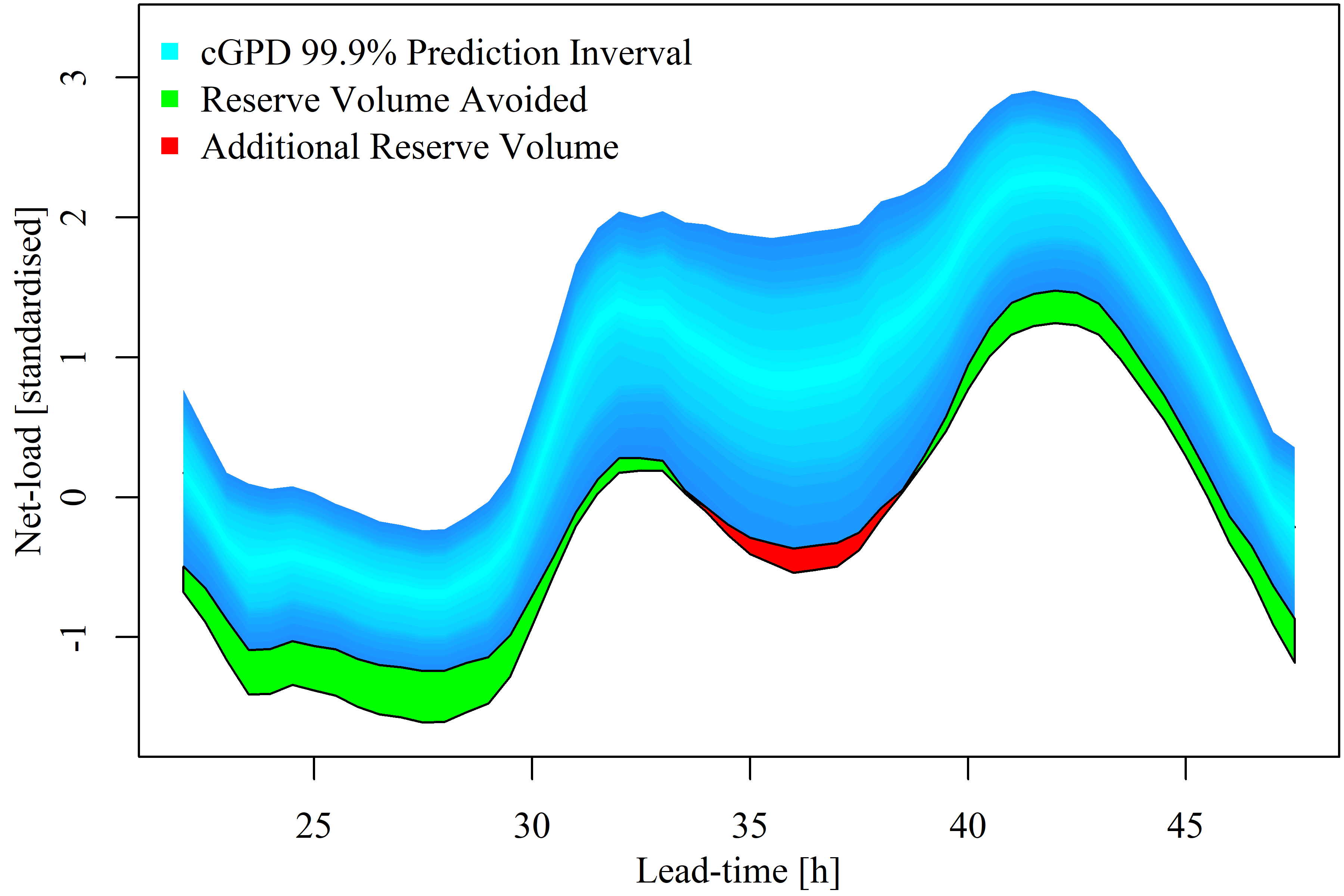
Figure 7: Illustration of the difference in reserve holding at 0.05% level between static and conditional GPD at GSP Group H. Compared to the sGPD, the cGPD requires less reserve to be held most of the time to maintaining the same risk level (green), but more reserve during period of greater uncertainty which the sGPD does not capture (red). Lead-time is hours since 2018-12-09T00:00:00Z.

VI Discussion and Conclusions

Predicting the possible extremes of future net electricity load is of interest to power system operators who must manage associated risks. However, this is challenging due to the inherent lack of data when modelling extremes, and the complexity introduced by embedded renewables. In this paper we have shown that the Generalised Pareto Distribution with a time-varying scale parameter can accurately describe the tails of predictive distributions. Time-variation is a result of conditioning the scale parameter on expected load and weather forecasts. The resulting forecasts are calibrated, unlike those produced by quantile regression, and sharper than those obtained using a non-time-varying approach.

Extensive evaluation has been performed based on data from the 14 regions of Great Britain’s electricity system, which exhibit a diversity of embedded wind and solar capacities relative to load. In addition to statistical measures, the practical task of reserve energy procurement to meet a given risk level has been considered. Conditioning the GPD allows forecasts to reflect changing uncertainty with the overall effect of reducing the volume of reserve required to achieve the target risk level. Importantly, while the overall volume of reserve is reduced relative to benchmarks by using the conditional GPD, during some periods reserve volume is higher, implying that the benchmarks expose users to excessive risk during these periods. The proposed method has the dual benefit of reducing cost and exposure to risk.

As part of this work we also studied the potential benefits of deriving weather features from gridded NWP to improve short-term net-load forecasts, as has been demonstrated for individual wind and solar farms. Gridded NWP does not appear to add significant value to deterministic and probabilistic net-load forecasts in the present framework, but it is possible that other forecasting methods would be able to extract value from this data by constructing different features, for example.

We have developed a complex model for net-load forecasting in GB with some GB-specific date/time features, however, the value of wind and solar-related weather features for net-load forecasting will be universal wherever the capacity of embedded wind and/or solar is significant. The model structure developed here, GAM with quantile regression and conditional parametric tails, should also generalise well to other applications. The problem of describing the tails of probabilistic forecasts that depend on covariates is certainly not unique to net-load forecasting, similar problems exist in meteorology, finance and logistics, for example.

Other future work should consider the spatio-temporal dependency between regions, and important aspect of energy system operation [37], and how this may depend on weather effects as the tails of predictive distribution do. Alternative approaches to predicting extremes of probabilistic net-load forecasts based on decomposing net-load into its constituent parts could also be considered. but would require careful modelling of potential tail dependency structures.

Jethro Browell received the M.Phys. degree in mathematics and theoretical physics from the University of St Andrews, U.K., in 2011, and the Ph.D. degree in wind energy systems from The University of Strathclyde, U.K., in 2015. He is a Senior Lecturer in the University of Strathclyde’s Institute for Energy and Environment where his research interests span all aspects of energy forecasting and associated decision-making in power system operation and energy markets. Dr. Browell is an EPSRC Innovation Fellow, a member of the IEEE Power & Energy Society and Vice-chair of the PES Working Group on Energy Forecasting and Analytics, and an editorial board member for Renewable and Sustainable Energy Reviews and Sustainable Energy, Grids and Networks.

Matteo Fasiolo received an M.Eng. degree in Industrial Engineering from the University of Udine, Italy, in 2010, an M.Sc in Financial Engineering from Birkbeck, University of London, U.K., in 2011, and a Ph.D. degree in Statistics from the University of Bath, U.K., in 2016. He is a Lecturer in the University of Bristol’s Institute for Statistical Science, where he works on developing non-parametric regression modelling methodology, with a particular focus on energy-related applications.

References

- [1] D. R. Drew, P. J. Coker, H. C. Bloomfield, D. J. Brayshaw, J. F. Barlow, and A. Richards, “Sunny windy sundays,” Renewable Energy, vol. 138, pp. 870–875, Aug 2019.
- [2] T. Hong and S. Fan, “Probabilistic electric load forecasting: A tutorial review,” International Journal of Forecasting, vol. 32, no. 3, pp. 914–938, Jul 2016.
- [3] P. Kobylinski, M. Wierzbowski, and K. Piotrowski, “High-resolution net load forecasting for micro-neighbourhoods with high penetration of renewable energy sources,” International Journal of Electrical Power & Energy Systems, vol. 117, p. 105635, May 2020.
- [4] D. van der Meer, J. Munkhammar, and J. Widén, “Probabilistic forecasting of solar power, electricity consumption and net load: Investigating the effect of seasons, aggregation and penetration on prediction intervals,” Solar Energy, vol. 171, pp. 397–413, Sep 2018.
- [5] M. Pierro, M. D. Felice, E. Maggioni, D. Moser, A. Perotto, F. Spada, and C. Cornaro, “Residual load probabilistic forecast for reserve assessment: A real case study,” Renewable Energy, vol. 149, pp. 508–522, Apr 2020.
- [6] T. Hong, P. Pinson, S. Fan, H. Zareipour, A. Troccoli, and R. J. Hyndman, “Probabilistic energy forecasting: Global energy forecasting competition 2014 and beyond,” International Journal of Forecasting, vol. 32, no. 3, pp. 896–913, 7 2016.
- [7] T. Li, Y. Wang, and N. Zhang, “Combining probability density forecasts for power electrical loads,” IEEE Transactions on Smart Grid, vol. 11, no. 2, pp. 1679–1690, Mar 2020.
- [8] Y. Chu, H. T. Pedro, A. Kaur, J. Kleissl, and C. F. Coimbra, “Net load forecasts for solar-integrated operational grid feeders,” Solar Energy, vol. 158, pp. 236–246, Dec 2017.
- [9] J. Andrade, J. Filipe, M. Reis, and R. Bessa, “Probabilistic price forecasting for day-ahead and intraday markets: Beyond the statistical model,” Sustainability, vol. 9, no. 11, p. 1990, 2017.
- [10] J. Xie and T. Hong, “Variable selection methods for probabilistic load forecasting: Empirical evidence from seven states of the united states,” IEEE Transactions on Smart Grid, vol. 9, no. 6, pp. 6039–6046, Nov 2018.
- [11] R. Moreno, M. Panteli, P. Mancarella, H. Rudnick, T. Lagos, A. Navarro, F. Ordonez, and J. C. Araneda, “From reliability to resilience: Planning the grid against the extremes,” IEEE Power and Energy Magazine, vol. 18, no. 4, pp. 41–53, Jul 2020.
- [12] M. Panteli and P. Mancarella, “Modeling and evaluating the resilience of critical electrical power infrastructure to extreme weather events,” IEEE Systems Journal, vol. 11, no. 3, pp. 1733–1742, Sep 2017.
- [13] S. Coles, An introduction to statistical modeling of extreme values. London New York: Springer, 2001.
- [14] C. Gonçalves, L. Cavalcante, M. Brito, R. J. Bessa, and J. Gama, “Forecasting conditional extreme quantiles for wind energy,” Electric Power Systems Research, vol. 190, p. 106636, 2021.
- [15] B. D. Youngman, “evgam: An R package for generalized additive extreme value models,” 2020, arXiv:2003.04067.
- [16] M. Matos and R. Bessa, “Setting the operating reserve using probabilistic wind power forecasts,” Power Systems, IEEE Transactions on, vol. 26, no. 2, pp. 594–603, May 2011.
- [17] H. Holttinen, M. Milligan, E. Ela, N. M. andJan Dobschinski, B. Rawn, R. J. Bessa, D. Flynn, E. Gómez-Lázaro, and N. K. Detlefsen, “Methodologies to determine operating reserves due to increased wind power,” IEEE Transactions on Sustainable Energy, vol. 3, no. 4, pp. 713–723, 2012.
- [18] N. Rajbhandari, W. Li, P. Du, S. Sharma, and B. Blevins, “Analysis of net-load forecast error and new methodology to determine non-spin reserve service requirement,” in 2016 IEEE Power and Energy Society General Meeting (PESGM). IEEE, Jul 2016.
- [19] P. Gaillard, Y. Goude, and R. Nedellec, “Additive models and robust aggregation for GEFCom2014 probabilistic electric load and electricity price forecasting,” International Journal of Forecasting, vol. 32, no. 3, pp. 1038–1050, Jul 2016.
- [20] T. Hong, P. Pinson, and S. Fan, “Global energy forecasting competition 2012,” International Journal of Forecasting, vol. 30, no. 2, pp. 357–363, Apr 2014.
- [21] R. A. Rigby and D. M. Stasinopoulos, “Generalized additive models for location, scale and shape,” Journal of the Royal Statistical Society: Series C (Applied Statistics), vol. 54, no. 3, pp. 507–554, 2005.
- [22] S. Wood, Generalized Additive Models: An Introduction with R (2nd edition). Chapman and Hall/CRC, 2017.
- [23] M. Fasiolo, S. N. Wood, M. Zaffran, R. Nedellec, and Y. Goude, “Fast calibrated additive quantile regression,” Journal of the American Statistical Association, pp. 1–11, Mar 2020.
- [24] J. R. Andrade and R. J. Bessa, “Improving renewable energy forecasting with a grid of numerical weather predictions,” IEEE Transactions on Sustainable Energy, vol. 8, no. 4, pp. 1571–1580, Oct 2017.
- [25] F. Ziel, “Modeling public holidays in load forecasting: a german case study,” Journal of Modern Power Systems and Clean Energy, vol. 6, no. 2, pp. 191–207, Feb 2018.
- [26] R. Koenker, Quantile Regression. Cambridge University Press, 2008.
- [27] S. N. Wood, N. Pya, and B. Säfken, “Smoothing parameter and model selection for general smooth models,” Journal of the American Statistical Association, vol. 111, no. 516, pp. 1548–1563, 2016.
- [28] T. Gneiting, F. Balabdaoui, and A. E. Raftery, “Probabilistic forecasts, calibration and sharpness,” Journal of the Royal Statistical Society: Series B (Statistical Methodology), vol. 69, pp. 243–268, 2007.
- [29] S. van Buuren and M. Fredriks, “Worm plot: a simple diagnostic device for modelling growth reference curves,” Statistics in Medicine, vol. 20, no. 8, pp. 1259–1277, 2001.
- [30] P. Pinson, P. McSharry, and H. Madsen, “Reliability diagrams for non-parametric density forecasts of continuous variables: Accounting for serial correlation,” Quarterly Journal of the Royal Meteorological Society, vol. 136, no. 646, pp. 77–90, Jan 2010.
- [31] J. Browell and M. Fasiolo. Supplementary material for “Probabilistic forecasitng of regional net-load with conditional extremes and gridded NWP”. [Online]. Available: https://doi.org/10.5281/zenodo.4618056
- [32] National Grid ESO. National Grid ESO Data Portal. [Online]. Available: https://data.nationalgrideso.com/
- [33] “Local authority districts (December 2017) super generalised clipped boundaries in Great Britain.” [Online]. Available: www.ons-inspire.esriuk.com
- [34] Office for National Statistics, “United Kingdom population mid-year estimate.” [Online]. Available: https://www.ons.gov.uk/
- [35] Solar Sheffield, “Solar Sheffield PV Live.” [Online]. Available: https://www.solar.sheffield.ac.uk/pvlive/
- [36] F. X. Diebold and R. S. Mariano, “Comparing predictive accuracy,” Journal of Business & Economic Statistics, vol. 13, no. 3, pp. 253–263, Jul 1995.
- [37] E. N. Martinez, N. Cutululis, and P. Sørensen, “High dimensional dependence in power systems: A review,” Renewable and Sustainable Energy Reviews, vol. 94, pp. 197–213, Oct 2018.
- [38] J. Browell and C. Gilbert, “ProbCast: Open-source production, evaluation and visualisation of probabilistic forecasts,” in Probabilistic Methods Applied to Power Systems Conference, 2020.