Error Prediction of Douglas-Rachford Algorithm for Linear Inverse Problems: Asymptotics of Proximity Operator for Squared Loss

Abstract

Proximal splitting-based convex optimization is a promising approach to linear inverse problems because we can use some prior knowledge of the unknown variables explicitly. An understanding of the behavior of the optimization algorithms would be important for the tuning of the parameters and the development of new algorithms. In this paper, we first analyze the asymptotic property of the proximity operator for the squared loss function, which appears in the update equations of some proximal splitting methods for linear inverse problems. The analysis shows that the output of the proximity operator can be characterized with a scalar random variable in the large system limit. Moreover, we investigate the asymptotic behavior of the Douglas-Rachford algorithm, which is one of the famous proximal splitting methods. From the resultant conjecture, we can predict the evolution of the mean squared error (MSE) in the algorithm for large-scale linear inverse problems. Simulation results demonstrate that the MSE performance of the Douglas-Rachford algorithm can be well predicted by the analytical result in compressed sensing with the $\ell_{1}$ optimization.

I Introduction

Linear inverse problems, i.e., the reconstruction of an unknown vector from its linear measurements, often appear in the field of signal processing. The linear inverse problem is called underdetermined when the number of measurements is less than that of elements of the unknown vector. In such underdetermined problems, we often use some prior knowledge of the unknown vector to obtain a good reconstruction result. In compressed sensing [1, 2, 3, 4], for example, we reconstruct an unknown sparse vector from its underdetermined linear measurements by using the sparsity effectively. Another example of the underdetermined problems is the overloaded signal detection in wireless communications [5, 6], where we can use the discreteness of the unknown vector.

A common approach to underdetermined linear inverse problems is to solve an optimization problem using some regularizer based on the prior knowledge of the unknown vector. In compressed sensing, the most popular optimization problem is the $\ell_{1}$ optimization, which utilizes the $\ell_{1}$ norm as the regularizer to promote the sparsity. Although the objective function is not differentiable due to the $\ell_{1}$ norm, some proximal splitting methods, e.g., the iterative soft thresholding algorithm (ISTA) [7, 8, 9] and the fast iterative soft thresholding algorithm (FISTA) [10], can solve the problem with feasible computational complexity. Alternating direction method of multipliers (ADMM) [11, 12] and the Douglas-Rachford algorithm [13, 14, 15] can also be applied to the $\ell_{1}$ optimization problem. Although these algorithms require a matrix inversion for linear inverse problems, they can converge faster than some gradient-based methods such as ISTA in some cases [16, 17].

The asymptotic performance of the final estimate by several optimization-based approaches for linear inverse problems has been analyzed by using some techniques [18, 19, 20]. In particular, the recently developed convex Gaussian min-max theorem (CGMT) [21, 22] enables us to obtain the asymptotic error in a precise manner for the optimizer of various optimization problems. For example, the asymptotic mean-square-error (MSE) of various regularized estimators has been analyzed in [23, 24]. The asymptotic symbol error rate has also been analyzed for the discrete-valued vector reconstruction in [24, 25].

The above analyses have focused on the performance of the optimizer, whereas the application of CGMT for the performance prediction of optimization algorithms has been considered in [26]. In [26], we have proposed a prediction method for the error performance of the tentative estimate at each iteration of ADMM. Such performance prediction could be utilized to understand the behavior of the algorithm, tune the parameter, and develop a new algorithm. For optimization algorithms other than ADMM, however, such asymptotic performance prediction has not been discussed for linear inverse problems in the literature.

In this paper, we investigate the asymptotic behavior of the Douglas-Rachford algorithm for linear inverse problems. In the analysis, we consider the objective function with the squared loss function and a separable regularizer. Since the proximity operator of the squared loss function is not element-wise, we investigate its asymptotic property via the CGMT framework. Specifically, we show that the output of the proximity operator for the squared loss function can be regarded as a scalar random variable in the large system limit. We then utilize the result to propose a prediction method for the evolution of the asymptotic MSE in the Douglas-Rachford algorithm. Although the derivation of the proposed method is partly non-rigorous, simulation results show that the empirical performance of the Douglas-Rachford algorithm is close to its prediction in compressed sensing with the $\ell_{1}$ optimization.

In this paper, we use the following notations. We denote the transpose by $(\cdot)^{\top}$ and the identity matrix by $\bm{I}$. For a vector $\bm{u}=\left[u_{1}\,\cdots\,u_{N}\right]^{\top}\in\mathbb{R}^{N}$, the $\ell_{1}$ norm and the $\ell_{2}$ norm are given by $\left\lVert\bm{u}\right\rVert_{1}=\sum_{n=1}^{N}\left\lvert u_{n}\right\rvert$ and $\left\lVert\bm{u}\right\rVert_{2}=\sqrt{\sum_{n=1}^{N}u_{n}^{2}}$, respectively. $\mathrm{sign}(\cdot)$ denotes the sign function. For a lower semicontinuous convex function $\phi:\mathbb{R}^{N}\to\mathbb{R}\cup\left\{+\infty\right\}$, we define the proximity operator as $\mathrm{prox}_{\phi}(\bm{u})=\operatornamewithlimits{\mathrm{arg\ min}}_{\bm{s}\in\mathbb{R}^{N}}\left\{\phi(\bm{s})+\frac{1}{2}\left\lVert\bm{s}-\bm{u}\right\rVert_{2}^{2}\right\}$. The Gaussian distribution with mean $\mu$ and variance $\sigma^{2}$ is denoted as $\mathcal{N}(\mu,\sigma^{2})$. When a sequence of random variables $\left\{\Theta_{n}\right\}$ ($n=1,2,\dotsc$) converges in probability to $\Theta$, we denote $\Theta_{n}\xrightarrow{\mathrm{P}}\Theta$ as $n\to\infty$ or $\operatornamewithlimits{\mathrm{plim}}_{n\to\infty}\Theta_{n}=\Theta$.

II Douglas-Rachford Algorithm
for Linear Inverse Problems

In this paper, we consider the linear inverse problem, i.e., the reconstruction of an $N$ dimensional vector $\bm{x}=\left[x_{1}\ \dotsb\ x_{N}\right]^{\top}\in\mathbb{R}^{N}$ from its linear measurements given by

$$\bm{y}=\bm{A}\bm{x}+\bm{v}\in\mathbb{R}^{M}.$$ (1)

Here, $\bm{A}\in\mathbb{R}^{M\times N}$ is a known measurement matrix and $\bm{v}\in\mathbb{R}^{M}$ is an additive noise vector. We mainly focus on the underdetermined case with $\Delta\coloneqq M/N<1$, where the solution is not unique even in the noiseless case. A common approach in such a case is to use the structure of $\bm{x}$ as the prior knowledge in the reconstruction. One of the most popular structures is sparsity, which means that most elements of $\bm{x}$ are zero. In some applications, the unknown vector has other structures such as boundedness and discreteness [27, 28].

Convex optimization is a promising approach to underdetermined linear inverse problems because we can flexibly design the objective function to utilize the structure of the unknown vector $\bm{x}$. In this paper, we consider the convex optimization problem given by

$$\operatornamewithlimits{\mathrm{minimize}}_{\bm{s}\in\mathbb{R}^{N}}\ \left\{L(\bm{s})+\lambda f({\bm{s}})\right\},$$ (2)

where we call $L(\bm{s})=\frac{1}{2}\left\lVert\bm{y}-\bm{A}\bm{s}\right\rVert_{2}^{2}$ as the squared loss function in this paper. The function $f(\cdot):\mathbb{R}^{N}\to\mathbb{R}\cup\left\{+\infty\right\}$ is a convex regularizer to utilize the prior knowledge of the unknown vector $\bm{x}$. For example, $\ell_{1}$ regularization $f(\bm{s})=\left\lVert\bm{s}\right\rVert_{1}$ is a popular convex regularizer for the reconstruction of a sparse vector. The regularization parameter $\lambda$ ($>0$) controls the balance between the squared loss function $L(\bm{s})$ and the regularization term $\lambda f({\bm{s}})$.

The Douglas-Rachford algorithm [13, 15] solves the optimization problem in (2) by using the proximity operators of $L(\cdot)$ and $f(\cdot)$. The update equations of the algorithm with the iteration index $k$ ($=0,1,2,\dotsc$) can be written as

$$\bm{s}^{(k+1)} =\mathrm{prox}_{\gamma L}\left(\bm{z}^{(k)}\right),$$ (3)

$$\bm{z}^{(k+1)} =\bm{z}^{(k)}+\rho_{k}\left(\mathrm{prox}_{\gamma\lambda f}\left(2\bm{s}^{(k+1)}-\bm{z}^{(k)}\right)-\bm{s}^{(k+1)}\right),$$ (4)

where $\gamma$ ($>0$) and $\rho_{k}\in[\varepsilon,2-\varepsilon]$ ($\varepsilon\in(0,1)$) are the parameters in the algorithm. By definition, the proximity operator of the function $L(\cdot)$ is given by

$$\mathrm{prox}_{\gamma L}\left(\bm{z}\right) =\operatornamewithlimits{\mathrm{arg\ min}}_{\bm{s}\in\mathbb{R}^{N}}\left\{\frac{1}{2}\left\lVert\bm{y}-\bm{A}\bm{s}\right\rVert_{2}^{2}+\frac{1}{2\gamma}\left\lVert\bm{s}-\bm{z}\right\rVert_{2}^{2}\right\}$$ (5)

$$=\left(\bm{A}^{\top}\bm{A}+\frac{1}{\gamma}\bm{I}\right)^{-1}\left(\bm{A}^{\top}\bm{y}+\frac{1}{\gamma}\bm{z}\right),$$ (6)

where $\bm{z}\in\mathbb{R}^{N}$ and $\gamma>0$. The proximity operator of $f(\cdot)$ can also be computed efficiently for various regularizers. When $f(\bm{s})=\left\lVert\bm{s}\right\rVert_{1}$, for example, the proximity operator of the function $f(\cdot)$ can be written as

$$\left[\mathrm{prox}_{\gamma\lambda f}(\bm{r})\right]_{n} =\mathrm{sign}(r_{n})\max(\left\lvert r_{n}\right\rvert-\gamma\lambda,0),$$ (7)

where $\bm{r}=\left[r_{1}\ \dotsb\ r_{N}\right]^{\top}\in\mathbb{R}^{N}$, and $\left[\cdot\right]_{n}$ denotes the $n$-th element of the vector. By computing (3) and (4) iteratively, we can obtain a sequence $\left\{\bm{s}^{(k)}\right\}_{k=1,2,\dotsc}$ converging to the solution of the optimization problem in (2).

III Main Results

III-A Asymptotics of Proximity Operator for Squared Loss

We firstly analyze the output of the proximity operator $\mathrm{prox}_{\gamma L}(\cdot)$ in (6). In the analysis, we assume the large system limit $M,N\to\infty$ ($M/N=\Delta$), where we consider the sequence of problems with $\left\{\bm{x},\bm{A},\bm{v}\right\}$ indexed by $N$ as in several high-dimensional analyses [22]. We also use the following assumption.

Assumption III.1.

The unknown vector $\bm{x}\in\mathbb{R}^{N}$ consists of independent and identically distributed (i.i.d.) random variables with a known distribution $p_{X}$ with some finite mean and variance. The measurement matrix $\bm{A}\in\mathbb{R}^{M\times N}$ consists of i.i.d. Gaussian random variables with zero mean and variance $1/N$. Moreover, the additive noise vector $\bm{v}\in\mathbb{R}^{M}$ is also Gaussian with zero mean and the covariance matrix $\sigma_{\text{v}}^{2}\bm{I}$.

Remark III.1.

In Assumption III.1, we assume that the elements of the measurement matrix $\bm{A}$ are Gaussian variables. This is because we require the Gaussian assumption in the CGMT-based analysis [22]. However, the universality of random matrices [29, 30, 31] suggests that the analytical result is valid when the measurement matrix is drawn from some other distributions.

Under Assumption III.1, we can obtain the following result on the asymptotic behavior of the proximity operator $\mathrm{prox}_{\gamma L}(\cdot)$.

Proposition III.1.

We assume that $\bm{x}$, $\bm{A}$, and $\bm{v}$ satisfy Assumption III.1. We consider the output of the proximity operator given by

$$\hat{\bm{s}} =\mathrm{prox}_{\gamma L}\left(\bm{z}\right),$$ (8)

where $\bm{z}$ has i.i.d. elements with a distribution $p_{Z}(z)$ and is assumed to be independent of $\bm{A}$. We here assume that the optimization problem

$$\min_{\alpha>0}\max_{\beta\geq 0}\left\{\frac{\alpha\beta\sqrt{\Delta}}{2}+\frac{\beta\sigma_{\text{v}}^{2}\sqrt{\Delta}}{2\alpha}-\frac{1}{2}\beta^{2}+\mathrm{E}\left[J(\alpha,\beta;Z)\right]\right\}$$ (9)

has a unique optimizer $(\alpha^{\ast},\beta^{\ast})$, where we define

$$J(\alpha,\beta;Z) =\frac{\beta\sqrt{\Delta}}{2\alpha}\left(\hat{S}(\alpha,\beta;Z)-X\right)^{2}$$

$$\hskip 11.38109pt-\beta H\left(\hat{S}(\alpha,\beta;Z)-X\right)$$

$$\hskip 11.38109pt+\frac{1}{2\gamma}\left(\hat{S}(\alpha,\beta;Z)-Z\right)^{2},$$ (10)

$$\hat{S}(\alpha,\beta;Z) =\dfrac{1}{\dfrac{\beta\sqrt{\Delta}}{\alpha}+\dfrac{1}{\gamma}}\left(\frac{\beta\sqrt{\Delta}}{\alpha}\left(X+\dfrac{\alpha}{\sqrt{\Delta}}H\right)+\frac{1}{\gamma}Z\right)$$ (11)

with the random variables $X\sim p_{X}$, $H\sim\mathcal{N}(0,1)$, and $Z\sim p_{Z}$. In (9), the expectation is taken over all random variables $X$, $H$, and $Z$. Then, the following statements hold:

1. The asymptotic MSE of $\hat{\bm{s}}$ in (8) is given by

   $$\operatornamewithlimits{\mathrm{plim}}_{M,N\to\infty}\frac{1}{N}\left\lVert\hat{\bm{s}}-\bm{x}\right\rVert_{2}^{2} =\left(\alpha^{\ast}\right)^{2}-\sigma_{\text{v}}^{2}.$$ (12)

2. Let $\mu_{\hat{\bm{s}}}$ be the empirical distribution of $\hat{\bm{s}}=\left[\hat{s}_{1}\ \dotsb\ \hat{s}_{N}\right]^{\top}\in\mathbb{R}^{N}$ corresponding to the cumulative distribution function (CDF) given by $P_{\hat{\bm{s}}}=\frac{1}{N}\sum_{n=1}^{N}\mathbb{I}\left(\hat{s}_{n}<s\right)$, where $\mathbb{I}\left(\hat{s}_{n}<s\right)=1$ if $\hat{s}_{n}<s$ and otherwise $\mathbb{I}\left(\hat{s}_{n}<s\right)=0$. Then, the distribution $\mu_{\hat{\bm{s}}}$ converges weakly in probability to the distribution $\mu_{S}$ of $S=\hat{S}\left(\alpha^{\ast},\beta^{\ast};Z\right)$, i.e., $\int gd\mu_{\hat{\bm{s}}}\xrightarrow{\mathrm{P}}\int gd\mu_{S}$ holds for any continuous compactly supported function $g(\cdot):\mathbb{R}\to\mathbb{R}$.

Sketch of proof.

By definition, the vector $\bm{s}$ is characterized as the solution of the optimization problem (5). Similarly to [25], we can prove the statement of the proposition by using the standard approach with CGMT [22]. We thus omit the details of the proof. For the overview of the derivation of (9), see Supplementary Material. ∎

The first statement in Proposition III.1 means that the asymptotic MSE for the output of the proximity operator can be predicted by solving the scalar optimization problem in (9). The second one implies that the distribution of the elements of the vector $\hat{\bm{s}}$ can be characterized by the random variable $S=\hat{S}\left(\alpha^{\ast},\beta^{\ast};Z\right)$. We can thus consider $\hat{S}\left(\alpha^{\ast},\beta^{\ast};Z\right)$ in (11) as a decoupled version of the proximity operator in (8) intuitively.

The optimization of $\alpha$ and $\beta$ in (9) can usually be performed by using searching techniques such as the ternary search and the golden section search [32]. Since the exact computation of the expectation in (9) is difficult in general, we need to approximate it with the average of many realizations of $X$, $H$, and $Z$.

III-B Application to Performance Prediction of Douglas-Rachford Algorithm

By using Proposition III.1, we propose a prediction method for the asymptotic behavior of the tentative estimate $\bm{s}^{(k)}$ in the Douglas-Rachford algorithm. In the derivation of the prediction method, we assume the separability of the regularizer $f(\cdot)$ as follows.

Assumption III.2.

Let the regularizer $f(\cdot):\mathbb{R}^{N}\to\mathbb{R}\cup\left\{+\infty\right\}$ be a lower semicontinuous convex function. Moreover, we assume that $f(\cdot)$ is separable and can be expressed as $f(\bm{s})=\sum_{n=1}^{N}\tilde{f}(s_{n})$ with a function $\tilde{f}(\cdot):\mathbb{R}\to\mathbb{R}\cup\left\{+\infty\right\}$. With the slight abuse of notation, we sometimes use the same $f(\cdot)$ for the corresponding function $\tilde{f}(\cdot)$.

Under Assumptions III.1 and III.2, we have the following conjecture. Note that the derivation of the conjecture is partly non-rigorous as [26, Claim III.1].

Conjecture III.1.

Suppose that Assumptions III.1 and III.2 hold. We consider the stochastic process given by

$$S_{k+1} =\hat{S}\left(\alpha_{k}^{\ast},\beta_{k}^{\ast};Z_{k}\right)$$ (13)

$$Z_{k+1} =Z_{k}+\rho_{k}\left(\mathrm{prox}_{\gamma\lambda f}\left(2S_{k+1}-Z_{k}\right)-S_{k+1}\right)$$ (14)

with the index $k$. We here assume that the optimization problem

$$\min_{\alpha>0}\max_{\beta\geq 0}\left\{\frac{\alpha\beta\sqrt{\Delta}}{2}+\frac{\beta\sigma_{\text{v}}^{2}\sqrt{\Delta}}{2\alpha}-\frac{1}{2}\beta^{2}+\mathrm{E}\left[J(\alpha,\beta;Z_{k})\right]\right\}$$ (15)

has a unique optimizer $(\alpha_{k}^{\ast},\beta_{k}^{\ast})$. Then, we have the following conjecture:

1. The asymptotic MSE of the tentative estimate $\bm{s}^{(k+1)}$ in (3) is given by

   $$\operatornamewithlimits{\mathrm{plim}}_{M,N\to\infty}\frac{1}{N}\left\lVert\bm{s}^{(k+1)}-\bm{x}\right\rVert_{2}^{2} =\left(\alpha_{k}^{\ast}\right)^{2}-\sigma_{\text{v}}^{2}.$$ (16)

2. The empirical distribution of $\bm{s}^{(k+1)}$ converges weakly in probability to the distribution of $S_{k+1}$.

Outline of derivation.

Since $\bm{z}^{(k)}$ in (3) and (4) is not independent of $\bm{A}$, Proposition III.1 cannot be used to (3) directly. We thus take the same procedure as the approach in [26, Claim III.1], where an unproven extension of CGMT has been assumed for the performance prediction of iterative algorithms. Under the assumption, the distribution of the element of $\bm{s}^{(k+1)}$ in (3) can be characterized by that of the random variable $S_{k+1}$ in (13) as in Proposition III.1 when the element of $\bm{z}^{(k)}$ can be regarded as the random variable $Z_{k}$. As for (4), the update of $\bm{z}^{(k)}$ can be decoupled into (14) because the update is element-wise under Assumption III.2. Since the procedure of the derivation is the same as [26, Claim III.1], the detailed explanation for the derivation is omitted. ∎

Conjecture III.1 implies that the evolution of the asymptotic MSE in the Douglas-Rachford algorithm can be predicted by solving the optimization problem in (15) and computing (16) for each $k$. The updates of $S_{k}$ and $Z_{k}$ in (13) and (14) can be considered as a decoupled version of the update of $\bm{s}^{(k)}$ and $\bm{z}^{(k)}$ in (3) and (4), respectively.

From the result in Conjecture III.1, we can tune the parameters in the Douglas-Rachford algorithm to achieve fast convergence. Since the relation between the parameters and the MSE is complicated, it is difficult to obtain the explicit expression of the optimal parameters. However, we can numerically predict the performance of the algorithm and select the parameter achieving fast convergence in the asymptotic regime.

IV Simulation Results

In this section, we demonstrate the validity of our approach via computer simulations. We consider an unknown vector $\bm{x}$ whose distribution is given by the Bernoulli-Gaussian distribution as

$$p_{X}(x) =p_{0}\delta_{0}(x)+(1-p_{0})p_{H}(x),$$ (17)

where $p_{0}\in(0,1)$ is the probability for $0$, $\delta_{0}(\cdot)$ denotes the Dirac delta function, and $p_{H}(\cdot)$ is the probability density function of the standard Gaussian distribution. The unknown vector $\bm{x}$ is sparse when $p_{0}$ is large. For the reconstruction of such sparse vector, we consider the $\ell_{1}$ optimization with $f(\bm{s})=\left\lVert\bm{s}\right\rVert_{1}$, i.e.,

$$\operatornamewithlimits{\mathrm{minimize}}_{\bm{s}\in\mathbb{R}^{N}}\left\{\frac{1}{2}\left\lVert\bm{y}-\bm{A}\bm{s}\right\rVert_{2}^{2}+\lambda\left\lVert\bm{s}\right\rVert_{1}\right\},$$ (18)

which is the most popular convex optimization problem for compressed sensing and satisfies Assumption III.2. In the simulations, the measurement matrix $\bm{A}$ and the noise vector $\bm{v}$ satisfy Assumption III.1.

We compare the empirical MSE performance of the Douglas-Rachford algorithm for (18) and its prediction obtained from Conjecture III.1. Figure 1 shows that the MSE performance versus the number of iterations in the algorithm, where $\Delta=0.7$, $p_{0}=0.9$, and $\sigma_{\text{v}}^{2}=0.001$.

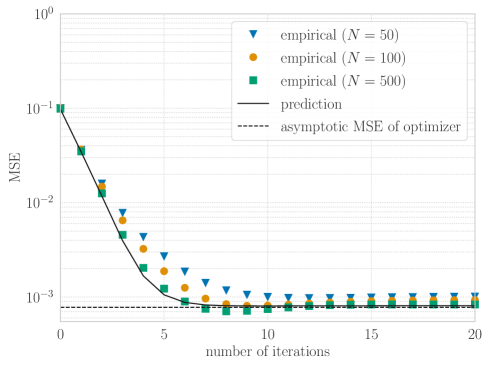
Figure 1: MSE performance for different $N$ in sparse vector reconstruction ($\Delta=0.7$, $p_{0}=0.9$, $\sigma_{\text{v}}^{2}=0.001$, $\gamma=10$, $\rho_{k}=1$).

The parameters of the Douglas-Rachford algorithm are set as $\gamma=10$ and $\rho_{k}=1$. The initial value of $\bm{z}^{(k)}$ is given by $\bm{z}^{(0)}=\bm{0}$. In the figure, ‘empirical’ denotes the empirical MSE performance of the Douglas-Rachford algorithm in (3) and (4) when $N=50,100$, and $500$. The empirical performance is obtained by averaging the results for $500$ independent realizations of $\bm{x}$, $\bm{A}$, and $\bm{v}$. Also, ‘prediction’ represents the performance prediction obtained by Conjecture III.1 in the large system limit. To obtain the prediction, we compute $300,000$ realizations of the random variables $(S_{k},Z_{k})$ and obtain the approximation of $(\alpha_{k}^{\ast},\beta_{k}^{\ast})$ because the exact computation of the distribution of $(S_{k},Z_{k})$ is difficult. As a reference, we also show the asymptotic MSE of the optimizer of the optimization problem in (18), which can be obtained from the standard CGMT approach as in [22]. The parameter $\lambda$ in (18) is determined by minimizing the asymptotic MSE of the optimizer. Figure 1 shows that the empirical performance is close to the prediction when $N$ is sufficiently large. We can also see that they converge to the asymptotic MSE of the optimizer of the $\ell_{1}$ optimization problem. To be precise, there is a slight difference between the empirical performance and its prediction. This is partly because we evaluate the empirical performance for finite $N$, whereas we assume the large system limit $N\to\infty$ in the asymptotic prediction. Another reason might be that we use many realizations of $(S_{k},Z_{k})$ for the prediction instead of computing their exact distributions.

Next, we evaluate the MSE performance for different parameters $\gamma$ in the Douglas-Rachford algorithm. Figure 2 shows the MSE performance versus $\gamma$, where $N=500$, $M=350$, $p_{0}=0.9$, $\sigma_{\text{v}}^{2}=0.001$, and $\rho_{k}=1$.

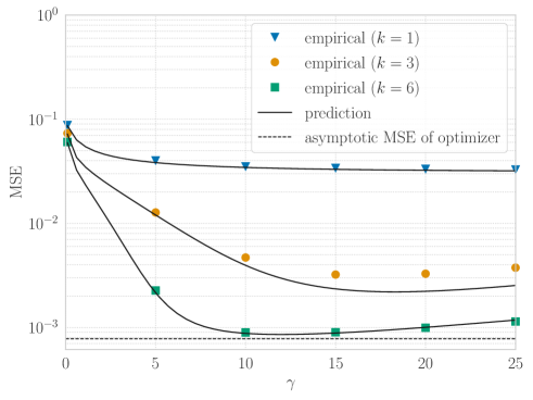
Figure 2: MSE performance versus $\gamma$ in sparse vector reconstruction ($N=500$, $M=350$, $p_{0}=0.9$, $\sigma_{\text{v}}^{2}=0.001$, $\rho_{k}=1$).

From the figure, we can observe that the performance is improved as the iteration index $k$ increases. The figure also implies that the value of $\gamma$ significantly affects the performance of the algorithm. Since the empirical performance is well predicted for all $\gamma$, we can tune the parameter by using the prediction. The figure shows that we should choose $\gamma$ between $10$ and $15$ in this case. Although the parameter $\rho_{k}$ is fixed in this paper for simplicity, we can also tune $\rho_{k}$ by using the prediction.

V Conclusion

In this paper, we have analyzed the asymptotic behavior of the proximity operator for the squared loss function in linear inverse problems. We have also shown that the result in Proposition III.1 can be used for the asymptotic performance prediction of the Douglas-Rachford algorithm for large-scale linear inverse problems. Simulation results show that the empirical performance of the Douglas-Rachford algorithm can be well predicted in large-scale compressed sensing with hundreds of unknown variables.

Appendix A Derivation of (9)

In this supplementary material, we provide an overview of the derivation of the optimization problem (9) from (5). Since the procedure is almost the same as the CGMT-based analyses [22, 25, 26], the rigorous discussion is omitted in some parts.

We define the error vector $\bm{e}=\bm{s}-\bm{x}$ to rewrite the optimization problem (5) as

$$\min_{\bm{e}\in\mathbb{R}^{N}}\frac{1}{N}\left\{\frac{1}{2}\left\lVert\bm{A}\bm{e}-\bm{v}\right\rVert_{2}^{2}+\frac{1}{2\gamma}\left\lVert\bm{e}+\bm{x}-\bm{z}\right\rVert_{2}^{2}\right\},$$ (19)

where the objective function is normalized by $N$. By using $\frac{1}{2}\left\lVert\bm{A}\bm{e}-\bm{v}\right\rVert_{2}^{2}=\max_{\bm{u}\in\mathbb{R}^{M}}\left\{\sqrt{N}\bm{u}^{\top}(\bm{A}\bm{e}-\bm{v})-\frac{N}{2}\left\lVert\bm{u}\right\rVert_{2}^{2}\right\}$, we can obtain the optimization problem

$$\min_{\bm{e}\in\mathbb{R}^{N}}\max_{\bm{u}\in\mathbb{R}^{M}}\Biggl{\{}\frac{1}{N}\bm{u}^{\top}(\sqrt{N}\bm{A})\bm{e}-\frac{1}{\sqrt{N}}\bm{v}^{\top}\bm{u}$$

$$\hskip 71.13188pt-\frac{1}{2}\left\lVert\bm{u}\right\rVert_{2}^{2}+\frac{1}{N}\frac{1}{2\gamma}\left\lVert\bm{e}+\bm{x}-\bm{z}\right\rVert_{2}^{2}\Biggr{\}}.$$ (20)

CGMT [22] enables us to analyze the optimization problem

$$\min_{\bm{e}\in\mathbb{R}^{N}}\max_{\bm{u}\in\mathbb{R}^{M}}\Biggl{\{}\frac{1}{N}\left(\left\lVert\bm{e}\right\rVert_{2}\bm{g}^{\top}\bm{u}-\left\lVert\bm{u}\right\rVert_{2}\bm{h}^{\top}\bm{e}\right)-\frac{1}{\sqrt{N}}\bm{v}^{\top}\bm{u}$$

$$\hskip 71.13188pt-\frac{1}{2}\left\lVert\bm{u}\right\rVert_{2}^{2}+\frac{1}{N}\frac{1}{2\gamma}\left\lVert\bm{e}+\bm{x}-\bm{z}\right\rVert_{2}^{2}\Biggr{\}}$$ (21)

instead of (20), where $\bm{g}\in\mathbb{R}^{M}$ and $\bm{h}\in\mathbb{R}^{N}$ are composed of i.i.d. standard Gaussian variables. Since both $\bm{g}$ and $\bm{v}$ are Gaussian, the vector $\frac{\left\lVert\bm{e}\right\rVert_{2}}{\sqrt{N}}\bm{g}-\bm{v}$ is also Gaussian with zero mean and the covariance matrix $\left(\frac{\left\lVert\bm{e}\right\rVert_{2}^{2}}{N}+\sigma_{\text{v}}^{2}\right)\bm{I}$. Hence, we can rewrite $\left(\frac{\left\lVert\bm{e}\right\rVert_{2}}{\sqrt{N}}\bm{g}-\bm{v}\right)^{\top}\bm{u}$ as $\sqrt{\frac{\left\lVert\bm{e}\right\rVert_{2}^{2}}{N}+\sigma_{\text{v}}^{2}}\bm{g}^{\top}\bm{u}$ with the slight abuse of notation, where $\bm{g}$ has i.i.d. standard Gaussian elements. We can thus obtain

$$\min_{\bm{e}\in\mathbb{R}^{N}}\max_{\bm{u}\in\mathbb{R}^{M}}\Biggl{\{}\frac{1}{\sqrt{N}}\sqrt{\frac{\left\lVert\bm{e}\right\rVert_{2}^{2}}{N}+\sigma_{\text{v}}^{2}}\bm{g}^{\top}\bm{u}-\frac{1}{N}\left\lVert\bm{u}\right\rVert_{2}\bm{h}^{\top}\bm{e}$$

$$\hskip 71.13188pt-\frac{1}{2}\left\lVert\bm{u}\right\rVert_{2}^{2}+\frac{1}{N}\frac{1}{2\gamma}\left\lVert\bm{e}+\bm{x}-\bm{z}\right\rVert_{2}^{2}\Biggr{\}}.$$ (22)

When we define $\beta=\left\lVert\bm{u}\right\rVert_{2}$, the maximum value of $\bm{g}^{\top}\bm{u}$ in the first term is given by $\beta\left\lVert\bm{g}\right\rVert_{2}$. Moreover, we use

$$\sqrt{\frac{\left\lVert\bm{e}\right\rVert_{2}^{2}}{N}+\sigma_{\text{v}}^{2}} =\min_{\alpha>0}\left(\frac{\alpha}{2}+\frac{\frac{\left\lVert\bm{e}\right\rVert_{2}^{2}}{N}+\sigma_{\text{v}}^{2}}{2\alpha}\right)$$ (23)

to transform the square root term in (22) as

$$\min_{\bm{e}\in\mathbb{R}^{N}}\max_{\beta\geq 0}\min_{\alpha>0}\Biggl{\{}\frac{\alpha\beta}{2}\frac{\left\lVert\bm{g}\right\rVert_{2}}{\sqrt{N}}+\frac{1}{N}\frac{\beta}{2\alpha}\frac{\left\lVert\bm{g}\right\rVert_{2}}{\sqrt{N}}\left\lVert\bm{e}\right\rVert_{2}^{2}+\frac{\beta\sigma_{\text{v}}^{2}}{2\alpha}\frac{\left\lVert\bm{g}\right\rVert_{2}}{\sqrt{N}}$$

$$\hskip 42.67912pt-\frac{\beta}{N}\bm{h}^{\top}\bm{e}-\frac{1}{2}\beta^{2}+\frac{1}{N}\frac{1}{2\gamma}\left\lVert\bm{e}+\bm{x}-\bm{z}\right\rVert_{2}^{2}\Biggr{\}}.$$ (24)

We can further rewrite (24) as

$$\min_{\alpha>0}\max_{\beta\geq 0}\Biggl{\{}\frac{\alpha\beta}{2}\frac{\left\lVert\bm{g}\right\rVert_{2}}{\sqrt{N}}+\frac{\beta\sigma_{\text{v}}^{2}}{2\alpha}\frac{\left\lVert\bm{g}\right\rVert_{2}}{\sqrt{N}}-\frac{1}{2}\beta^{2}$$

$$\hskip 85.35826pt+\min_{\bm{e}\in\mathbb{R}^{N}}\frac{1}{N}\sum_{n=1}^{N}J_{n}(e_{n},\alpha,\beta)\Biggr{\}},$$ (25)

where the subscript $(\cdot)_{n}$ denotes the $n$-th element of the corresponding bold vector and $J_{n}(e_{n},\alpha,\beta)=\frac{\beta}{2\alpha}\frac{\left\lVert\bm{g}\right\rVert_{2}}{\sqrt{N}}e_{n}^{2}-\beta h_{n}e_{n}+\frac{1}{2\gamma}\left(e_{n}+x_{n}-z_{n}\right)^{2}$. The minimum value of $J_{n}(e_{n},\alpha,\beta)$ over $e_{n}$ is given by $J_{n}(\hat{s}_{n}(\alpha,\beta)-x_{n},\alpha,\beta)$, where

$$\hat{s}_{n}(\alpha,\beta)=\dfrac{1}{\dfrac{\beta}{\alpha}\dfrac{\left\lVert\bm{g}\right\rVert_{2}}{\sqrt{N}}+\dfrac{1}{\gamma}}\Biggl{(}\frac{\beta}{\alpha}\frac{\left\lVert\bm{g}\right\rVert_{2}}{\sqrt{N}}\left(x_{n}+\frac{\sqrt{N}}{\left\lVert\bm{g}\right\rVert_{2}}\alpha h_{n}\right)+\frac{1}{\gamma}z_{n}\Biggr{)}.$$ (26)

Hence, the optimization problem (25) can be rewritten as

$$\min_{\alpha>0}\max_{\beta\geq 0}\Biggl{\{}\frac{\alpha\beta}{2}\frac{\left\lVert\bm{g}\right\rVert_{2}}{\sqrt{N}}+\frac{\beta\sigma_{\text{v}}^{2}}{2\alpha}\frac{\left\lVert\bm{g}\right\rVert_{2}}{\sqrt{N}}-\frac{1}{2}\beta^{2}$$

$$\hskip 56.9055pt+\frac{1}{N}\sum_{n=1}^{N}J_{n}\left(\hat{s}_{n}(\alpha,\beta)-x_{n},\alpha,\beta\right)\Biggr{\}}.$$ (27)

We can show the objective function of (27) converges pointwise to (9) as $M,N\to\infty$. $J_{n}(\hat{s}_{n}(\alpha,\beta)-x_{n},\alpha,\beta)$ and $\hat{s}_{n}(\alpha,\beta)$ correspond to (10) and (11), respectively.

Intuitively, from the definition of $\alpha$ in (23), the optimal value of $\alpha$ corresponds to $\sqrt{\frac{\left\lVert\bm{e}\right\rVert_{2}^{2}}{N}+\sigma_{\text{v}}^{2}}$, which finally results in (12). For the precise discussion, see [22, 25].

References

- [1] E. J. Candès and T. Tao, “Decoding by linear programming,” IEEE Trans. Inf. Theory, vol. 51, no. 12, pp. 4203–4215, Dec. 2005.
- [2] E. J. Candès, J. Romberg, and T. Tao, “Robust uncertainty principles: Exact signal reconstruction from highly incomplete frequency information,” IEEE Trans. Inf. Theory, vol. 52, no. 2, pp. 489–509, Feb. 2006.
- [3] D. L. Donoho, “Compressed sensing,” IEEE Trans. Inf. Theory, vol. 52, no. 4, pp. 1289–1306, Apr. 2006.
- [4] E. J. Candès, “The restricted isometry property and its implications for compressed sensing,” Comptes Rendus Mathematique, vol. 346, no. 9, pp. 589–592, May 2008.
- [5] H. Sasahara, K. Hayashi, and M. Nagahara, “Multiuser detection based on MAP estimation with sum-of-absolute-values relaxation,” IEEE Trans. Signal Process., vol. 65, no. 21, pp. 5621–5634, Nov. 2017.
- [6] R. Hayakawa and K. Hayashi, “Convex optimization-based signal detection for massive overloaded MIMO systems,” IEEE Trans. Wirel. Commun., vol. 16, no. 11, pp. 7080–7091, Nov. 2017.
- [7] I. Daubechies, M. Defrise, and C. D. Mol, “An iterative thresholding algorithm for linear inverse problems with a sparsity constraint,” Commun. Pure Appl. Math., vol. 57, no. 11, pp. 1413–1457, 2004.
- [8] P. L. Combettes and V. R. Wajs, “Signal recovery by proximal forward-backward splitting,” Multiscale Model. Simul., vol. 4, no. 4, pp. 1168–1200, Jan. 2005.
- [9] M. A. T. Figueiredo, R. D. Nowak, and S. J. Wright, “Gradient projection for sparse reconstruction: Application to compressed sensing and other inverse problems,” IEEE J. Sel. Top. Signal Process., vol. 1, no. 4, pp. 586–597, Dec. 2007.
- [10] A. Beck and M. Teboulle, “A fast iterative shrinkage-thresholding algorithm for linear inverse problems,” SIAM J. Imaging Sci., vol. 2, no. 1, pp. 183–202, Jan. 2009.
- [11] D. Gabay and B. Mercier, “A dual algorithm for the solution of nonlinear variational problems via finite element approximation,” Computers & Mathematics with Applications, vol. 2, no. 1, pp. 17–40, Jan. 1976.
- [12] S. Boyd, N. Parikh, E. Chu, B. Peleato, and J. Eckstein, “Distributed optimization and statistical learning via the alternating direction method of multipliers,” Found Trends Mach Learn, vol. 3, no. 1, pp. 1–122, Jan. 2011.
- [13] P. Lions and B. Mercier, “Splitting algorithms for the sum of two nonlinear operators,” SIAM J. Numer. Anal., vol. 16, no. 6, pp. 964–979, Dec. 1979.
- [14] J. Eckstein and D. P. Bertsekas, “On the Douglas-Rachford splitting method and the proximal point algorithm for maximal monotone operators,” Mathematical Programming, vol. 55, no. 1, pp. 293–318, Apr. 1992.
- [15] P. L. Combettes and J.-C. Pesquet, “Proximal splitting methods in signal processing,” in Fixed-Point Algorithms for Inverse Problems in Science and Engineering, ser. Springer Optimization and Its Applications. New York, NY: Springer New York, 2011, vol. 49, pp. 185–212.
- [16] P. L. Combettes and L. E. Glaudin, “Fully proximal splitting algorithms in image recovery,” in Proc. 27th European Signal Processing Conference (EUSIPCO), Sep. 2019, pp. 1–5.
- [17] ——, “Proximal activation of smooth functions in splitting algorithms for convex image recovery,” SIAM J. Imaging Sci., vol. 12, no. 4, pp. 1905–1935, Jan. 2019.
- [18] D. L. Donoho, A. Maleki, and A. Montanari, “The noise-sensitivity phase transition in compressed sensing,” IEEE Trans. Inf. Theory, vol. 57, no. 10, pp. 6920–6941, Oct. 2011.
- [19] M. Bayati and A. Montanari, “The LASSO risk for Gaussian matrices,” IEEE Trans. Inf. Theory, vol. 58, no. 4, pp. 1997–2017, Apr. 2012.
- [20] D. L. Donoho, I. Johnstone, and A. Montanari, “Accurate prediction of phase transitions in compressed sensing via a connection to minimax denoising,” IEEE Trans. Inf. Theory, vol. 59, no. 6, pp. 3396–3433, Jun. 2013.
- [21] C. Thrampoulidis, A. Panahi, and B. Hassibi, “Asymptotically exact error analysis for the generalized -LASSO,” in Proc. IEEE International Symposium on Information Theory (ISIT), Jun. 2015, pp. 2021–2025.
- [22] C. Thrampoulidis, E. Abbasi, and B. Hassibi, “Precise error analysis of regularized -estimators in high dimensions,” IEEE Trans. Inf. Theory, vol. 64, no. 8, pp. 5592–5628, Aug. 2018.
- [23] I. B. Atitallah, C. Thrampoulidis, A. Kammoun, T. Y. Al-Naffouri, M. Alouini, and B. Hassibi, “The BOX-LASSO with application to GSSK modulation in massive MIMO systems,” in Proc. IEEE International Symposium on Information Theory (ISIT), Jun. 2017, pp. 1082–1086.
- [24] C. Thrampoulidis, W. Xu, and B. Hassibi, “Symbol error rate performance of box-relaxation decoders in massive MIMO,” IEEE Trans. Signal Process., vol. 66, no. 13, pp. 3377–3392, Jul. 2018.
- [25] R. Hayakawa and K. Hayashi, “Asymptotic performance of discrete-valued vector reconstruction via box-constrained optimization with sum of regularizers,” IEEE Trans. Signal Process., vol. 68, pp. 4320–4335, 2020.
- [26] R. Hayakawa, “Asymptotic performance prediction for ADMM-based compressed sensing,” IEEE Trans. Signal Process., vol. 70, pp. 5194–5207, 2022.
- [27] P. H. Tan, L. K. Rasmussen, and T. J. Lim, “Constrained maximum-likelihood detection in CDMA,” IEEE Trans. Commun., vol. 49, no. 1, pp. 142–153, Jan. 2001.
- [28] M. Nagahara, “Discrete signal reconstruction by sum of absolute values,” IEEE Signal Process. Lett., vol. 22, no. 10, pp. 1575–1579, Oct. 2015.
- [29] M. Bayati, M. Lelarge, and A. Montanari, “Universality in polytope phase transitions and message passing algorithms,” Ann. Appl. Probab., vol. 25, no. 2, pp. 753–822, Apr. 2015.
- [30] A. Panahi and B. Hassibi, “A universal analysis of large-scale regularized least squares solutions,” in Proc. Advances in Neural Information Processing Systems, 2017, pp. 3381–3390.
- [31] S. Oymak and J. A. Tropp, “Universality laws for randomized dimension reduction, with applications,” Inf Inference, vol. 7, no. 3, pp. 337–446, Sep. 2018.
- [32] D. G. Luenberger and Y. Ye, “Basic Descent Methods,” in Linear and Nonlinear Programming, ser. International Series in Operations Research & Management Science. New York, NY: Springer US, 2008, pp. 215–262.