Learning to Schedule Heuristics in Branch-and-Bound

Abstract

Primal heuristics play a crucial role in exact solvers for Mixed Integer Programming (MIP). While solvers are guaranteed to find optimal solutions given sufficient time, real-world applications typically require finding good solutions early on in the search to enable fast decision-making. While much of MIP research focuses on designing effective heuristics, the question of how to manage multiple MIP heuristics in a solver has not received equal attention. Generally, solvers follow hard-coded rules derived from empirical testing on broad sets of instances. Since the performance of heuristics is instance-dependent, using these general rules for a particular problem might not yield the best performance. In this work, we propose the first data-driven framework for scheduling heuristics in an exact MIP solver. By learning from data describing the performance of primal heuristics, we obtain a problem-specific schedule of heuristics that collectively find many solutions at minimal cost. We provide a formal description of the problem and propose an efficient algorithm for computing such a schedule. Compared to the default settings of a state-of-the-art academic MIP solver, we are able to reduce the average primal integral by up to $49\%$ on a class of challenging instances.

1 Introduction

Many decision-making problems arising from real-world applications can be formulated using Mixed Integer Programming (MIP). The Branch-and-Bound (B&B) framework is a general approach to solving MIPs to global optimality. Over the recent years, the idea of using machine learning (ML) to improve optimization techniques has gained renewed interest. There exist various approaches to tackle different aspects of the solving process using classical ML techniques. For instance, ML has been used to find good parameter configurations for a solver [Hutter et al., 2009, Hutter et al., 2011], improve node [He et al., 2014], variable [Khalil et al., 2016, Nair et al., 2020] or cut [Baltean-Lugojan et al., 2019] selection strategies, and detect decomposable structures [Kruber et al., 2017].

Even though exact MIP solvers aim for global optimality, finding good feasible solutions fast is at least as important, especially in the presence of a time limit. The use of primal heuristics is crucial in ensuring good primal performance in modern solvers. For instance, [Berthold, 2013a] showed that the primal bound–the objective value of the best solution–improved on average by around $80\%$ when primal heuristics were used. Generally, a solver has a variety of primal heuristics implemented, where each class exploits a different idea to find good solutions. During B&B, these heuristics are executed successively at each node of the search tree, and improved solutions are reported back to the solver if found. Extensive overviews of different primal heuristics, their computational costs, and their impact in MIP solving can be found in [Lodi, 2013, Berthold, 2013b, Berthold, 2018].

Since most heuristics can be very costly, it is necessary to be strategic about the order in which the heuristics are executed and the number of iterations allocated to each, with the ultimate goal of obtaining good primal performance overall. Such decisions are often made by following hard-coded rules derived from testing on broad benchmark test sets. While these static settings yield good performance on average, their performance can be far from optimal when considering specific families of instances. To illustrate this fact, Figure 2 compares the success rates of different primal heuristics for two problem classes: the Generalized Independent Set Problem (GISP) [Hochbaum and Pathria, 1997, Colombi et al., 2017] and the Fixed-Charge Multicommodity Network Flow Problem (FCMNF) [Hewitt et al., 2010].

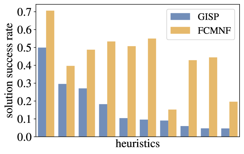
Figure 1: Average solution success rates of ten heuristics for two problem classes. Heuristic success is problem-dependent: each pair of blue-yellow bars belongs to one heuristic, and the heuristics are sorted in descending order w.r.t. the solution success rates for GISP (blue). The yellow bars representing the success rates for FCMNF are far from being sorted, implying that the performance of a heuristic is strongly problem-dependent.

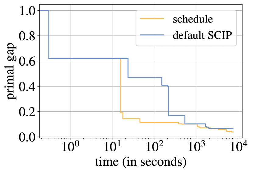
Figure 2: Primal gap for an exemplary GISP instance. Our method’s heuristic schedule (orange) obtains better solutions earlier than SCIP’s default (blue).

In this paper, we propose a data-driven approach to systematically improve the use of primal heuristics in B&B. By learning from data about the duration and success of every heuristic call for a set of training instances, we construct a schedule of heuristics deciding when and for how long a certain heuristic should be executed to obtain good primal solutions early on. As a result, we are able to significantly improve the use of primal heuristics which is shown in Figure 2 for one MIP instance.

Even through we will focus on improving primal performance of MIP solving, it is important to note that finding good solutions faster also improves the overall running time of the solver. The B&B procedure generates a search tree in which the nodes correspond to different subproblems. To determine whether a certain part of the tree should be further explored or pruned, we keep track of the incumbent, i.e., the best feasible solution seen thus far. Hence, when good incumbents are found early on, the size of the search tree may be significantly reduced, leading to the problem being solved faster. On a standardized test set, primal heuristics reduced the solving time by up to $30\%$ [Berthold, 2013a].

1. We formalize the learning task of finding an effective, cost-efficient heuristic schedule on a training dataset as a Mixed Integer Quadratic Program (see Section 3);

2. We propose an efficient heuristic for solving the training (scheduling) problem and a scalable data collection strategy (see Section 4 and 5);

3. We perform extensive computational experiments on a class of challenging instances and demonstrate the benefits of our approach (see Section 6).

Since primal heuristics have such a significant influence on the solving process, optimizing their usage is a topic of ongoing research. For instance, by characterizing nodes with different features, [Khalil et al., 2017] propose an ML method to decide at which nodes heuristics should run to improve primal performance. After that decision, all heuristics are executed according to the predefined rules set by the solver. The authors in [Hendel, 2018] and [Hendel et al., 2018] use bandit algorithms to learn from previous calls which heuristics to execute first. In contrast to the method proposed in this paper, their procedure only adapts the order in which heuristics are executed. Furthermore, primal performance can also be improved by using hyperparameter tuning [Hutter et al., 2009, Hutter et al., 2011], but generally come with extremely high computational cost, since they do not exploit information about the structure of the problem.

2 Preliminaries

Let us consider a MIP of the form

$$\underset{x\in\mathbb{R}^{n}}{\text{min}} c^{\mathsf{T}}x, P_{\textit{MIP}}$$ ()

s.t. $$Ax\leq b,$$

$$x_{i}\in\mathbb{Z},\quad\forall i\in I$$

with matrix $A\in\mathbb{R}^{m\times n}$, vectors $c\in\mathbb{R}^{n}$, $b\in\mathbb{R}^{m}$, and index set $I\subseteq[n]$. A MIP can be solved using Branch-and-Bound, a tree search algorithm that finds an optimal solution to ($P_{\textit{MIP}}$) by recursively partitioning the original problem into linear subproblems. The nodes in the resulting search tree correspond to these subproblems. Throughout this work, we assume that each node has a unique index that identifies the node even across branch-and-bound trees obtained for different MIP instances. For a set of instances $\mathcal{X}$, we denote the union of the corresponding node indices by $\mathcal{N}_{\mathcal{X}}$.

Primal Performance Metrics. Since we are interested in finding good solutions fast, we consider a collection of different metrics for primal performance. Beside statistics like the time to the first/best solution and the solution/incumbent success rate, we mainly focus on the primal integral [Berthold, 2013a] as a comprehensive measure of primal performance. Intuitively, this metric can be interpreted as a normalized average of the incumbent value over time. Formally, if $x$ is feasible and $x^{*}$ is an optimal (or best known) solution to ($P_{\textit{MIP}}$), the primal gap of $x$ is defined as

$$\gamma(x)\coloneqq\begin{cases}0,&\text{ if }|c^{\mathsf{T}}x|=|c^{\mathsf{T}}x^{*}|,\\ 1,&\text{ if }c^{\mathsf{T}}x\cdot c^{\mathsf{T}}x^{*}<0,\\ \dfrac{|c^{\mathsf{T}}x-c^{\mathsf{T}}x^{*}|}{\text{max}\{|c^{\mathsf{T}}x|,|c^{\mathsf{T}}x^{*}|\}},&\text{ otherwise}.\end{cases}$$

With $x^{t}$ denoting the incumbent at time $t$, the primal gap function $p:\mathbb{R}_{\geq 0}\to[0,1]$ is then defined as

$$p(t)\coloneqq\begin{cases}1,&\text{ if no incumbent is found until time }t,\\ \gamma(x^{t}),&\text{ otherwise}.\end{cases}$$

For a time limit $T\in\mathbb{R}_{\geq 0}$, the primal integral $P(T)$ is then given by the area underneath the primal gap function $p$ up to time $T$,

$$P(T)\coloneqq\sum_{i=1}^{K}p(t_{i-1})(t_{i}-t_{i-1}),$$

where $(K-1)$ incumbents have been found until time $T$, $t_{0}=0$, $t_{K}=T$, and $t_{1},\dots,t_{K-1}$ are the points in time at which new incumbents are found.

Figure 2 gives an example for the primal gap function. The primal integrals are the areas under each of the curves. It is easy to see that finding near-optimal incumbents earlier shrinks the area under the graph of $p$, resulting in a smaller primal integral.

3 Data-Driven Heuristic Scheduling

The performance of heuristics strongly depends on the set of problem instances they are applied to. Hence, it is natural to consider data-driven approaches for optimizing the use of primal heuristics for the instances of interest. Concretely, we consider the following practically relevant setting. We are given a set of heuristics $\mathcal{H}$ and a homogeneous set of training instances $\mathcal{X}$ from the same problem class. In a data collection phase, we are allowed to execute the B&B algorithm on the training instances, observing how each heuristic performs at each node of each search tree. At a high level, our goal is then to leverage this data to obtain a schedule of heuristics that minimizes a primal performance metric.

The specifics of how such data collection is carried out will be discussed later on in the paper. First, let us examine the decisions that could potentially benefit from a data-driven approach. Our discussion is inspired by an in-depth analysis of how the source-open academic MIP solver SCIP [Gamrath et al., 2020] manages primal heuristics. However, our approach is generic and is likely to apply to other MIP solvers.

3.1 Controlling the Order

One important degree of freedom in scheduling heuristics is the order in which a set of applicable heuristics $\mathcal{H}$ is executed by the solver at a given node. This can be controlled by assigning a priority for each heuristic. In a heuristic loop, the solver then iterates over the heuristics in decreasing priority. The loop is terminated if a heuristic finds a new incumbent solution. As such, an ordering $\langle h_{1},\dots,h_{k}\rangle$ that prioritizes effective heuristics can lead to time savings without sacrificing primal performance.

3.2 Controlling the Duration

Furthermore, solvers use working limits to control the computational effort spent on heuristics. Consider diving heuristics as an example. Increasing the maximal diving depth increases the likelihood of finding an integer feasible solution. At the same time, this increases the overall running time. Figure 3 visualizes this cost-benefit trade-off empirically for three different diving heuristics, highlighting the need for a careful “balancing act”.

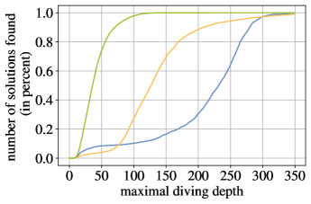
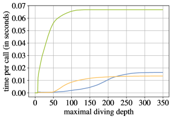
Figure 3: Number of solutions found (in percent) and cost of different diving heuristics depending on the the maximal diving depth: This figure shows the average number of solutions found by a heuristic (left) and average duration in seconds (right) of three diving heuristics when limiting the maximal depth of a dive. Hereby, the baseline for the values on the vertical axis of the left figure is the number of found solutions by the heuristics with no limitations on the diving depth. The likelihood of finding a solution increases with the maximal diving depth. At the same time, an average call to all three heuristics becomes more expensive as the diving depth increases.

For a heuristic $h\in\mathcal{H}$, let $\tau\in\mathbb{R}_{>0}$ denote $h$’s time budget. Then, we are interested in finding a schedule $S$ defined by

$$S\coloneqq\langle(h_{1},\tau_{1}),\dots,(h_{k},\tau_{k})\rangle,h_{i}\in\mathcal{H}.$$

Since controlling the time budget directly can be unreliable and lead to nondeterministic behavior in practice (see Appendix B for details), a deterministic proxy measure is preferable. For diving heuristics, the maximal diving depth provides a suitable measure as demonstrated by Figure 3. Similar measures can be used for other types of heuristics, as we will demonstrate with Large Neighborhood Search heuristics in Section 6. In general, we will refer to $\tau_{i}$ as the maximal number of iterations that is alloted to a heuristic $h_{i}$ in schedule $S$.

3.3 Deriving the Scheduling Problem

Having argued for order and duration as suitable control decisions, we will now formalize our heuristic scheduling problem. Ideally, we would like to construct a single schedule $S$ that minimizes the primal integral, as defined in Section 2, averaged over the training instances $\mathcal{X}$. Unfortunately, it is very difficult to optimize the primal integral directly, as it depends on the sequence of incumbents found over time during B&B. The primal integral also depends on the way the search tree is explored, which is affected by pruning, further complicating any attempt at directly optimizing this primal metric.

We address this difficulty by considering a more practical surrogate objective. Recall that $\mathcal{N}_{\mathcal{X}}$ denotes the collection of search tree nodes of the set of training instances $\mathcal{X}$. We will construct a schedule $S$ that finds feasible solutions for a large fraction of the nodes in $\mathcal{N}_{\mathcal{X}}$, while also minimizing the number of iterations spent by schedule $S$. Note that we consider feasible solutions instead of incumbents here: This way, we are able to obtain more data faster since a heuristic finds a feasible solution more often than a new incumbent. The framework we propose in the following can handle incumbents instead, but we have found no benefit in that in preliminary experiments.

For a heuristic $h\in\mathcal{H}$ and node $N$, denote by $t(h,N)$ the iterations necessary for $h$ to find a solution at node $N$, and set $t(h,N)=\infty$ if $h$ does not succeed at $N$. Now suppose a schedule $S$ is successful at node $N$, i.e., some heuristic finds a solution within the budget allocated to it in $S$. Let

$$j_{S}=\text{min}\{j=1,\ldots,|\mathcal{H}|\mid t(h_{j},N)\leq\tau_{j}\}$$

be the index of the first successful heuristic. Following the (successful) execution of $h_{j_{S}}$, the heuristic loop is terminated, and the time spent by schedule $S$ at node $N$ is given by

$$T(S,N)\coloneqq\sum_{i=1}^{j_{S}-1}\tau_{i}+t(h_{j_{S}},N).$$

Otherwise, set $T(S,N)\coloneqq\sum_{i=1}^{k}\tau_{i}+1$.

Furthermore, let $\mathcal{N}_{S}$ denote the set of nodes at which schedule $S$ is successful in finding a solution. Then, we consider the heuristic scheduling problem given by

$$\underset{S\in\mathcal{S}}{\text{min}}\sum_{N\in\mathcal{N}_{\mathcal{X}}}T(S,N)\;\text{ s.t. }\;|\mathcal{N}_{S}|\geq\alpha|\mathcal{N}_{\mathcal{X}}|. P_{\mathcal{S}}$$ ()

Here $\alpha\in[0,1]$ denotes a minimum fraction of nodes at which we want the schedule to find a solution. Problem ($P_{\mathcal{S}}$) can be formulated as a Mixed-Integer Quadratic Program (MIQP); the exact formulation can be found in Appendix A.

To find such a schedule, we need to know $t(h,N)$ for every heuristic $h$ and node $N$. Hence, when collecting data for the instances in the training set $\mathcal{X}$, we track for every B&B node $N$ at which a heuristic $h$ was called, the number of iterations $\tau_{N}^{h}$ it took $h$ to find a feasible solution; we set $\tau_{N}^{h}=\infty$ if $h$ does not succeed at $N$. Formally, we require a training dataset

$$\mathcal{D}\coloneqq\{(h,N,\tau_{N}^{h}))\mid h\in\mathcal{H},N\in\mathcal{N}_{\mathcal{X}},\tau_{N}^{h}\in\mathbb{R}_{+}\cup\{\infty\}\}.$$

Section 5 describes a computationally efficient approach for building $\mathcal{D}$ using a single B&B run per training instance.

4 Solving the Scheduling Problem

Problem ($P_{\mathcal{S}}$) is a generalization of the Pipelined Set Cover Problem which is known to be $\mathcal{NP}$-hard [Munagala et al., 2005]. As for the MIQP in Appendix A, tackling it using a non-linear integer programming solver is challenging: the MIQP has $O(|\mathcal{H}||\mathcal{N}_{\mathcal{X}}|)$ variables and constraints, and a single training instance may involve thousands of search tree nodes, leading to an MIQP with hundreds of thousands of variables and constraints even with a handful of heuristics and tens of training instances.

As already mentioned in the beginning, one approach to finding a schedule that heuristically solves ($P_{\mathcal{S}}$) is using a hyperparameter tuning software like SMAC [Hutter et al., 2011]. Since SMAC is a sequential algorithm that searches for a good parameter configuration by successively adapting and re-testing its best settings, training a SMAC schedule can get very expensive quickly. In the following, we present a more efficient approach.

We now direct our attention towards designing an efficient heuristic algorithm for ($P_{\mathcal{S}}$). A similar problem was studied by [Streeter, 2007] in the context of decision problems. Among other things, the author discusses how to find a schedule of (randomized) heuristics that minimizes the expected time necessary to solve a set of training instances $\mathcal{X}$ of a decision problem. Although this setting is somewhat similar to ours, there exist multiple aspects in which they differ significantly:

1. Decision problems are considered instead of MIPs: Solving a MIP is generally much more challenging than solving a decision problem. When solving a MIP with B&B, we normally have to solve many linear subproblems. Since in theory, every such LP is an opportunity for a heuristic to find a new incumbent, we consider the set of nodes $\mathcal{N}_{\mathcal{X}}$ instead of $\mathcal{X}$ as the “instances” we want to solve.

2. A heuristic call can be suspended and resumed: In the work of [Streeter, 2007], a heuristic can be executed in a “suspend-and-resume model”: If $h$ was executed before, the action $(h,\tau)$ represents continuing a heuristic run for an additional $\tau$ iterations. When $h$ reaches the iteration limit, the run is suspended and its state kept in memory such that it can be resumed later in the schedule. The “suspend-and-resume” model is not used in MIP solving due to challenges in maintaining the states of heuristics in memory. As such, we allow every heuristic to be included in the schedule at most once.

3. Time is used to control the duration of a heuristic run: Controlling time directly is unreliable in practice and can lead to nondeterministic behavior of the solver. Instead, we rely on different proxy measures for different classes of heuristics. Thus, when building a schedule that contains heuristics of distinct types (e.g., diving and LNS heuristics), we need to ensure that these measures are comparable.

Despite these differences, it is useful to examine the greedy scheduling approach proposed by [Streeter, 2007]. A schedule is built by successively adding the action $(h,\tau)$ to $G$ that maximizes the ratio of the marginal increase in the number of instances solved to the cost (i.e., $\tau$) of including $(h,\tau)$. As shown in Corollary 2 of [Streeter, 2007], the greedy schedule $G$ yields a 4-approximation of that version of the scheduling problem. In an attempt to leverage this elegant heuristic in our problem ($P_{\mathcal{S}}$), we will describe it formally.

Let us denote the greedy schedule by $G\coloneqq\langle g_{1},\dots,g_{k}\rangle$. Then, $G$ is defined inductively by setting $G_{0}=\langle\rangle$ and $G_{j}=\langle g_{1},\dots,g_{j}\rangle$ with

$$g_{j}=\underset{(h,\tau)\in\mathcal{H}_{j-1}\times\mathcal{T}}{\text{argmax}}\frac{|\{N\in\mathcal{N}_{\mathcal{X}}^{j-1}\mid\tau_{N}^{h}\leq\tau\}|}{\tau}.$$

Here, $\mathcal{H}_{i}$ denotes the set of heuristics that are not yet in $G_{i}$, $\mathcal{N}_{\mathcal{X}}^{i}$ denotes the subset of nodes where $G_{i}$ is not yet successful in finding a solution, and $\mathcal{T}$ is the interval generated by all possible iteration limits in $\mathcal{D}$, i.e.,

$$\mathcal{T}\coloneqq[\text{min}\{\tau_{N}^{h}\mid(N,h,\tau_{N}^{h})\in\mathcal{D}\},\text{max}\{\tau_{N}^{h}\mid(N,h,\tau_{N}^{h})\in\mathcal{D}\}].$$

We stop adding actions $g_{j}$ when $G_{j}$ finds a solution at all nodes in $\mathcal{N}_{\mathcal{X}}$ or all heuristics are contained in the schedule, i.e., $\mathcal{H}_{j}=\emptyset$.

Unfortunately, we can show that the resulting schedule can perform arbitrarily bad in our setting. Consider the following situation. We assume that there are 100 nodes in $\mathcal{N}_{\mathcal{X}}$ and only one heuristic $h$. This heuristic solves one node in just one iteration and takes 100 iterations each for the other 99 nodes. Following the greedy approach, the resulting schedule would be $G=\langle(h,1)\rangle$ since $\frac{1}{1}>\frac{99}{100}$. Whenever $\alpha>0.01$, $G$ would be infeasible for our constrained problem ($P_{\mathcal{S}}$). Since we are not allowed to add a heuristic more than once, this cannot be fixed with the current algorithm.

To avoid this situation, we propose the following modification. Instead of only considering the heuristics that are not in $G_{j-1}$ when choosing the next action $g_{j}$, we also consider the option to run the last heuristic $h_{j-1}$ of $G_{j-1}$ for longer. That is, we allow to choose $(h_{j-1},\tau)$ with $\tau>\tau_{j-1}$. Note that the cost of adding $(h_{j-1},\tau)$ to the schedule is not $\tau$, but $\tau-\tau_{j-1}$, since we decide to run $h_{j-1}$ for $\tau-\tau_{j-1}$ iterations longer and not to rerun $h_{j-1}$ for $\tau$ iterations.

Furthermore, when including different classes of heuristics in the schedule, the respective time measures are not necessarily comparable (see Figure 4). To circumvent this problem, we use the average time per iteration to normalize different notions of iterations. In the following, we denote the average cost of an iteration by $t^{h}_{avg}$ for heuristic $h$. Note that $t^{h}_{avg}$ can be easily computed by also tracking the duration (w.r.t. time) of a heuristic run in data collection.

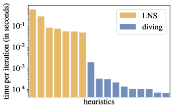
Figure 4: Comparison of average cost of iterations for different primal heuristics: While the cost of an iteration is relatively similar among heuristics of the same type, they differ significantly when comparing diving and LNS with each other. On average, an iteration for LNS heuristics (number of nodes in sub-MIP) is much more expensive than for diving heuristics (maximal diving depth).

Hence, we redefine $g_{j}$ and obtain

$$g_{j}=\underset{(h,\tau)\in\mathcal{A}_{j-1}}{\text{argmax}}\frac{|\{N\in\mathcal{N}_{\mathcal{X}}^{j-1}\mid\tau_{N}^{h}\leq\tau\}|}{c_{j-1}(h,\tau)},$$

with $\mathcal{A}_{i}\coloneqq(\mathcal{H}_{i}\times\mathcal{T})\cup\{(h_{i},\tau)\mid\tau>\tau_{i},\tau\in\mathcal{T}\}$ and

$$c_{i}(h,\tau)\coloneqq\begin{cases}t^{h}_{avg}\tau,&\text{ if $h\neq h_{i}$}\\ t^{h}_{avg}(\tau-\tau_{i}),&\text{ otherwise}.\end{cases}$$

We set $\mathcal{A}_{0}\coloneqq\mathcal{H}\times\mathcal{T}$ and $c_{0}(h,\tau)=t^{h}_{avg}\tau$. With this modification, we would obtain the schedule $G=\langle(h,100)\rangle$ (which solves all 100 nodes) in the above example.

Finally, note that this greedy procedure still does not explicitly enforce that the schedule is successful at a fraction of at least $\alpha$ nodes. In our experiments, however, we observe that the resultings schedules reach a success rate of $\alpha=98\%$ or above. The final formulation of the algorithm can be found in Algorithm 1.

Algorithm 1 Greedy algorithm to obtain a schedule

  Input: Nodes $\mathcal{N}_{\mathcal{X}}$, heuristics $\mathcal{H}$, data $D$, time frame $\mathcal{T}$

  Output: Greedy Schedule $G$

  $G\leftarrow\langle\rangle$

  $\mathcal{N}_{unsol}\leftarrow\mathcal{N}_{\mathcal{X}}$

  $improve\leftarrow$ TRUE

  repeat

     $(h^{*},\tau^{*})\leftarrow\underset{(h,\tau)\in\mathcal{A}}{\text{argmax}}\left[\frac{|\{N\in\mathcal{N}_{unsol}\mid\tau_{h}^{N}\leq\tau\}|}{c(h,\tau)}\right]$

     if $\frac{|\{N\in\mathcal{N}_{unsol}\mid\tau_{h^{*}}^{N}\leq\tau^{*}\}|}{c(h,\tau^{*})}>0$ then

        $G\leftarrow G\oplus\langle(h^{*},\tau^{*})\rangle$

        $\mathcal{N}_{unsol}\leftarrow\mathcal{N}_{unsol}\setminus\{N\in\mathcal{N}_{unsol}\mid\tau_{h^{*}}^{N}\leq\tau^{*}\}$

     else

        $improve\leftarrow$ FALSE

     end if

  until $improve==$ FALSE

Example. Figure 5 shows an example of how we obtain a schedule with three heurisitcs and nodes. As the left figure indicates, the data set is given by

$$\mathcal{D}=\{ (h_{1},N_{1},1),(h_{1},N_{2},\infty),(h_{1},N_{3},\infty),(h_{2},N_{1},4),(h_{2},N_{2},3),$$

$$(h_{2},N_{3},3),(h_{3},N_{1},\infty),(h_{3},N_{2},4),(h_{3},N_{3},2)\}.$$

Let us now assume that an iterations of each heuristic has the same average costs, i.e., $t^{h_{1}}_{avg}=t^{h_{2}}_{avg}=t^{h_{3}}_{avg}$, we build an schedule $G$ as follows. First, we add the action $(h_{1},1)$, since $h_{1}$ solves one node with only one iteration yielding a ratio that cannot be bet by the other heuristics. No other node can be solved by $h_{1}$, hence it does not have to be considered anymore, as well as node $N_{1}$. Among the remaining possibilities, the action $(h_{2},3)$ is the best, since $h_{2}$ solves both nodes in three iterations yielding a ratio of $\frac{2}{3}$. In contrast, executing $h_{3}$ for two and four iterations, respectively, would yield a ratio of $\frac{1}{2}$. Since this is smaller, we add $(h_{2},3)$ to the $G$ and obtain the schedule $G=\langle(h_{1},1),(h_{2},3)\rangle$ which solves all three nodes as shown on the right of Figure 5. It is easy to see that this schedule is an optimal solution of ($P_{\mathcal{S}}$) for $\alpha>\frac{1}{3}$.

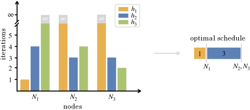
Figure 5: Example of how to obtain a heuristic schedule from data: The data is shown on the left for three heuristics and nodes and the (optimal) schedule obtained by following Algorithm 1 is illustrated on the right.

5 Data Collection

The scheduling approach described thus far rests on the availability of a training data set of the form

$$\mathcal{D}\coloneqq\{(h,N,\tau_{N}^{h})\mid h\in\mathcal{H},N\in\mathcal{N}_{\mathcal{X}},\tau_{N}^{h}\in\mathbb{R}_{+}\cup\{\infty\}\}.$$

In words, each entry in data set $\mathcal{D}$ is a triplet containing: the index of a heuristic $h$; the index of a B&B node $N$ coming from one of the training instances in $\mathcal{X}$; the number of iterations required by $h$ to find a feasible solution at the node $N$. The latter piece of information, $\tau_{N}^{h}$, must be collected by executing the heuristic and observing its performance. Two main challenges arise in collecting such a data set for multiple heuristics:

1. Efficient data collection: Solving $\mathcal{NP}$-hard MIPs by B&B remains computationally expensive, even given the sophisticated techniques implemented in today’s solvers. This poses difficulties to ML approaches that create a single reward signal from one MIP evaluation, which may take several minutes up to hours. This holds in particular for challenging problem classes that are the focus of this work. In other words, even with a handful of heuristics, i.e., a small set $\mathcal{H}$, it is prohibitive to run B&B once for each heuristic-training instance pair in order to construct the data set $\mathcal{D}$.

2. Obtaining unbiased data: On the other hand, executing multiple heuristics at each node of the search tree during data collection can have dangerous side effects: if a heuristic finds an incumbent, subsequent heuristics are no longer executed at the same node, as described in Section 3.1.

We address the first point by using a specially crafted version of the MIP solver for collecting multiple reward signals for the execution of multiple heuristics per single MIP evaluation during the training phase. As a result, we obtain a large amount of data points that scales with the running time of the MIP solves. This has the clear advantage that the efficiency of our data collection does not automatically decrease when the time to evaluate a single MIP increases for more challenging problems.

To address the second point and prevent bias from mutual interaction of different heuristic calls during training, we engineered the MIP solver to be executed in a special shadow mode, where heuristics are called in a sandbox environment and interaction with the main solving path is maximally reduced. In particular this means that new incumbents and primal bounds are not communicated back, but only recorded for training data. This setting is an improved version of the shadow mode introduced in [Khalil et al., 2017].

As a result of these measures, we have instrumented the SCIP solver in a way that allows for the collection of a proper data set $\mathcal{D}$ with a single run of the Branch-and-Bound algorithm per training instance.

6 Computational Results

We will now detail our computational results. The code we used for data collection and scheduling is publicly available .

6.1 Heuristics

We can build a schedule containing arbitrary heuristics as long as they have some type of time measure. In this work, we focus on two broad groups of heuristics: Diving and Large Neighborhood Search (LNS). Both classes are much more computationally expensive than simpler heuristics like rounding, but are generally also more likely to find (good) solutions [Berthold, 2006]. That is why it is particularly important to schedule these heuristics most economically.

Diving Heuristics. Diving heuristics examine a single probing path by successively fixing variables according to a specific rule. There are multiple ways of controlling the duration of a dive. After careful consideration of the different options, we decided on using the maximum diving depth to limit the cost of a call to a diving heuristic: It is both related to the effort spent by the heuristic and its likelihood of success.

LNS Heuristics. This class of heuristics first builds a neighborhood of some reference point which is then searched for improving solutions by solving a sub-MIP. To control the duration of a call to a LNS heuristic, we choose to limit the number of nodes in the sub-MIP. The idea behind this measure is similar to limiting the diving depth of diving heuristics: In both cases, we control the number of subproblems that a heuristic considers within its execution. Nevertheless, the two measures are not directly comparable, as shown in Figure 4.

To summarize, we use 16 primal heuristics in our schedule: ten diving and six LNS heuristics. By controlling this set, we cover the majority of the more complex heuristics implemented in SCIP. All other heuristics are executed after the schedule according to their default settings.

6.2 Instances

Since our goal is to improve the primal performance of a solver, we focus on a primally challenging problem class: The Generalized Independent Set Problem (GISP) [Hochbaum and Pathria, 1997, Colombi et al., 2017]. In the following, we will briefly explain how we generate and partition the instances.

Let $G=(V,E)$ be a graph and $E^{\prime}\subseteq E$ a subset of removable edges. Each vertex has a revenue and every edge has a cost associated with it. Then, GISP asks to select a subset of vertices and removable edges that maximizes the profit, i.e., the difference of vertex revenue and edge costs. Thereby, no edge should exist between two selected vertices $v,u\in V$, i.e., either we have that $(v,u)\notin E$ or $(v,u)\in E^{\prime}$ is removed.

We generate GISP instances in the following way. Given a graph, we randomize the set of removable edges by setting the probability that an edge is in $E^{\prime}$ to $\alpha=0.75$. Furthermore, we choose the revenue for each node to be $100$ and the cost of every edge as $1$. This results in a configuration for which it is difficult to find good feasible solutions as shown in [Colombi et al., 2017].

We use this scheme to generate two types of instances. The first one takes graphs from the 1993 DIMACS Challenge which is also used by [Khalil et al., 2017, Colombi et al., 2017]. Thereby, we focus on the same twelve dense graphs as well as the same train/test partition as in [Khalil et al., 2017]. The training set consists of six graphs with 125–300 nodes and 6963–20864 edges, whereas the testing graphs are considerably larger with 250–400 nodes and 21928–71819 edges. We generate 20 instances for every graph by using different random seeds, leaving us with 120 instances for training as well as testing. For the second group of GISP instances, we use randomly generated graphs where the number of nodes is uniformly chosen from $\{L,\dots,U\}$ for bounds $L,U\in\mathbb{N}$. An edge is added to the resulting graph with probability $\bar{\alpha}=0.1$, giving us slightly less dense graphs than the previous case. We denote these sets by [L,U]. For each set, we generate 25 instances for training and 10 for testing. The smallest set of graphs then has 150–160 nodes and 1099–1268 edges whereas the largest set consists of graphs with 550–560 nodes and 14932–15660 edges.

6.3 Results

To study the performance of our approach, we used the state-of-the-art solver SCIP 7.0 [Gamrath et al., 2020] with CPLEX 12.10.0.0 as the underlying LP solver. Thereby, we needed to modify SCIP’s source code to collect data as described in Section 5, as well as control heuristic parameters that are not already implemented by default. For our experiments, we used a Linux cluster of Intel Xeon CPU E5-2660 v3 2.60GHz with 25MB cache and 128GB main memory. The time limit in all experiments was set to two hours; for data collection, we used a time limit of four hours. Since the primal integral depends on time, we ran one process at a time on every machine, allowing for accurate on time measurements.

MIP solver performance can be highly sensitive to even small and seemingly performance-neutral perturbations during the solving process [Lodi and Tramontani, 2013], a phenomenon referred to as performance variability. We implemented a more exhaustive testing framework than the commonly used benchmark methodology in MIP that uses extensive cross-validation in addition to multiple random seeds.

In addition to comparing our scheduling method against default SCIP, we also compare against scip_tuned, a hand-tuned version of SCIP’s default settings for GISP. Since in practice, a MIP expert would try to manually optimize some parameters when dealing with a homogeneous set of instances, we emulated that process to create an even stronger baseline to compare our method against.

Random graph instances. Table 1 shows the results of the cross-validation experiments for schedules with diving heuristics. Our scheduling framework yields a significant improvement w.r.t. primal integral on all test sets. Since this improvement is consistent over all schedules and test sets, we are able to validate that the behavior actually comes from our procedure. Especially remarkable is the fact that the schedules trained on smaller instances also perform well on much larger instances.

Note that the instances in the first three test sets were solved to optimality by all settings whereas the remaining ones terminated after two hours without a provably optimal solution. When looking at the instances that were not solved to optimality, we can see that the schedules perform especially well on instances of increasing difficulty. This behavior is intuitive: Since our method aims to improve the primal performance of a solver, it performs better when an instance is very challenging on the primal side.

	[150,160]	[200,210]	[250,260]	[300,310]	[350,360]	[400,410]	[450,460]	[500,510]	[550,560]
[150,160]	$0.89\pm 0.23$	$0.76\pm 0.22$	$0.87\pm 0.37$	$0.95\pm 0.40$	$0.87\pm 0.28$	$0.86\pm 0.23$	$0.78\pm 0.24$	$0.80\pm 0.25$	$0.65\pm 0.24$
[200,210]	$0.94\pm 0.28$	$0.75\pm 0.25$	$0.82\pm 0.30$	$0.91\pm 0.34$	$0.93\pm 0.23$	$0.90\pm 0.28$	$0.83\pm 0.22$	$0.79\pm 0.20$	$0.66\pm 0.20$
[250,260]	$0.89\pm 0.28$	$0.69\pm 0.23$	$0.81\pm 0.34$	$0.94\pm 0.40$	$0.92\pm 0.23$	$0.96\pm 0.39$	$0.81\pm 0.24$	$0.76\pm 0.22$	$0.66\pm 0.20$
[300,310]	$0.87\pm 0.25$	$0.71\pm 0.26$	$0.83\pm 0.36$	$0.97\pm 0.39$	$0.92\pm 0.28$	$0.90\pm 0.35$	$0.81\pm 0.24$	$0.75\pm 0.24$	$0.61\pm 0.24$
[350,360]	$0.84\pm 0.24$	$0.70\pm 0.23$	$0.82\pm 0.36$	$0.91\pm 0.37$	$0.81\pm 0.26$	$0.86\pm 0.31$	$0.80\pm 0.21$	$0.75\pm 0.19$	$0.59\pm 0.20$
[400,410]	$0.90\pm 0.27$	$0.70\pm 0.23$	$0.83\pm 0.36$	$0.88\pm 0.32$	$0.77\pm 0.23$	$0.88\pm 0.30$	$0.81\pm 0.21$	$0.74\pm 0.20$	$0.58\pm 0.20$
[450,460]	$0.89\pm 0.25$	$0.70\pm 0.23$	$0.83\pm 0.36$	$0.88\pm 0.32$	$0.77\pm 0.23$	$0.88\pm 0.30$	$0.81\pm 0.21$	$0.74\pm 0.20$	$0.58\pm 0.20$
[500,510]	$0.89\pm 0.26$	$0.72\pm 0.22$	$0.84\pm 0.30$	$0.99\pm 0.42$	$0.92\pm 0.24$	$0.95\pm 0.46$	$0.81\pm 0.23$	$0.80\pm 0.25$	$0.61\pm 0.20$
[550,560]	$0.88\pm 0.26$	$0.72\pm 0.24$	$0.89\pm 0.42$	$0.95\pm 0.37$	$0.86\pm 0.27$	$0.90\pm 0.28$	$0.81\pm 0.20$	$0.78\pm 0.23$	$0.63\pm 0.21$
SCIP_TUNED	$0.89\pm 0.28$	$0.77\pm 0.23$	$0.99\pm 0.31$	$1.08\pm 0.45$	$1.05\pm 0.28$	$1.03\pm 0.38$	$0.94\pm 0.23$	$0.91\pm 0.28$	$0.76\pm 0.25$

Table 1: Average relative primal integral (mean $\pm$ std.) of schedule (with diving heuristics) w.r.t. default SCIP over GISP instances derived from random graphs. The first nine rows correspond to schedules that were trained on instances of size [l,u]

schedule	better primal integral	better primal bound
[150,160]	0.69	0.70
[200,210]	0.69	0.65
[250,260]	0.68	0.55
[300,310]	0.72	0.58
[350,360]	0.76	0.62
[400,410]	0.75	0.61
[450,460]	0.75	0.61
[500,510]	0.68	0.58
[550,560]	0.70	0.59

Table 2: Fraction of instances for which our method’s schedule (with diving heuristics) has a better primal integral/bound at termination w.r.t. scip_tuned. Only instances that were not solved to optimality by both scip_tuned and the schedule are considered in the second column.

Over all test sets, the schedules terminated with a strictly better primal integral on 69–76% and with a strictly better primal bound on 59–70% of the instances compared to scip_tuned (see Table 2).

Table 3 shows a part of the cross-validation experiments for schedules containing diving and LNS heuristics. As expected, including both classes of heuristics improves the overall performance of the schedule. In this case, the improvement is only marginal since on the instances we consider, diving seems to perform significantly better than LNS.

	[150,160]	[200,210]	[250,260]	[300,310]	[350,360]
[150,160]	$0.84\pm 0.19$	$0.65\pm 0.29$	$0.89\pm 0.35$	$0.91\pm 0.32$	$0.88\pm 0.28$
[200,210]	$0.87\pm 0.16$	$0.76\pm 0.33$	$0.91\pm 0.32$	$0.93\pm 0.34$	$0.89\pm 0.29$
[250,260]	$0.83\pm 0.18$	$0.71\pm 0.34$	$0.89\pm 0.31$	$0.90\pm 0.29$	$0.87\pm 0.32$
[300,310]	$0.81\pm 0.19$	$0.62\pm 0.24$	$0.91\pm 0.42$	$0.92\pm 0.32$	$0.94\pm 0.32$
[350,360]	$0.82\pm 0.19$	$0.61\pm 0.25$	$0.84\pm 0.42$	$0.86\pm 0.23$	$0.86\pm 0.28$
SCIP_TUNED	$0.89\pm 0.28$	$0.77\pm 0.23$	$0.99\pm 0.31$	$1.08\pm 0.45$	$1.05\pm 0.28$

Table 3: Average relative primal integral (mean $\pm$ std.) of schedule (with diving and LNS heuristics) w.r.t. default SCIP over GISP instances derived from random graphs. The first five rows correspond to schedules that were trained on instances of size [l,u]. On highlighted entries, a schedule controling both diving and LNS performs better than its diving counterpart (see Table 1). More intense colors denote higher improvement.

Finding a schedule with SMAC. As mentioned before, we can also find a schedule by using the hyperparameter tuning tool SMAC. To test SMAC’s performance on the random graph instances, we trained ten SMAC schedules on a selection of the nine training sets. To make it easier for SMAC, we only considered diving heuristics in this case. For the sake of comparability, we gave SMAC the same total computational time for training as we did in data collection: With 25 training instances per set and a time limit of four hours, this comes to 100 hours per training set and schedule. Note that since SMAC runs sequentially, training the SMAC schedules took over four days per schedule, whereas training a schedule following the greedy algorithm only took four hours with enough machines. To pick the best performing SMAC schedule for each training set, we ran all ten schedules on the test set of same size as the corresponding training set and chose the best performing one to also run on the other test sets.

The results can be found in Table 4. As we can see, on all test sets, all schedules are significantly better than default SCIP. However, when comparing these results to the performance of the greedy schedules (see Table 1), we can see that SMAC performs worse on average. Over all five test sets, the SMAC schedules terminated with a strictly better primal integral on 36 – 54% and with a strictly better primal bound on 37 – 55% of the instances.

	[150,160]	[250,260]	[350,360]	[450,460]	[550,560]		compared to schedule
							better primal integral	better primal bound
[150,160]	$0.81\pm 0.23$	$0.77\pm 0.34$	$0.90\pm 0.27$	$0.85\pm 0.24$	$0.65\pm 0.19$		0.49	0.37
[250,260]	$0.87\pm 0.26$	$0.88\pm 0.42$	$0.87\pm 0.25$	$0.83\pm 0.24$	$0.59\pm 0.22$		0.52	0.53
[350,360]	$0.86\pm 0.24$	$0.80\pm 0.37$	$0.86\pm 0.25$	$0.80\pm 0.24$	$0.68\pm 0.18$		0.47	0.42
[450,460]	$0.93\pm 0.26$	$0.87\pm 0.32$	$0.90\pm 0.19$	$0.85\pm 0.25$	$0.69\pm 0.23$		0.36	0.44
[550,560]	$0.87\pm 0.22$	$0.83\pm 0.31$	$0.92\pm 0.29$	$0.84\pm 0.26$	$0.58\pm 0.21$		0.54	0.55
scip_tuned	$0.89\pm 0.28$	$0.77\pm 0.23$	$0.99\pm 0.31$	$1.08\pm 0.45$	$1.05\pm 0.28$		-	-

Table 4: Average relative primal integral (mean $\pm$ std.) of SMAC schedule w.r.t. default SCIP and the fraction of instances for which the SMAC schedule has a better primal integral/bound at termination w.r.t. the greedy schedule over GISP instances derived from random graphs. The first five rows correspond to schedules (with diving heuristics) that were trained with SMAC on instances of size [l,u]. On highlighted entries, a SMAC schedule performs better than its greedy counterpart (see Table 1). More intense colors denote higher improvement. Only instances that were not solved to optimality by both SMAC and the greedy schedule are considered in the last column.

DIMACS graph instances. Table 5 summarizes the results on the instances derived from DIMACS graphs. To stay consistent with [Khalil et al., 2017], we only schedule diving heuristics. As we can see, the schedule setting dominates default SCIP in all metrics, but an especially drastic improvement can be obtained w.r.t. the primal integral: the schedule reduces the primal integral by 49%.

When looking at the total time spent in heuristics, we see that heuristics run significantly shorter but with more success: On average, the incumbent success rate is higher compared to default SCIP.

	DEFAULT	SCIP_TUNED	SCHEDULE
Primal Integral	$934.48$	$555.75$	$470.73$
Time to first Incumbent	$1.33$	$1.33$	$1.26$
Time to best Incumbent	$4266.68$	$2642.46$	$2803.38$
Best Incumbent	$2382.03$	$2385.73$	$2404.63$
Total heuristic calls*	$138.57$	$137.38$	$140.03$
Total heuristic time*	$258.88$	$304.96$	$190.10$
Number of Incumbents found*	$2.72$	$3.08$	$3.33$
Incumbent Success Rate*	$0.01$	$0.02$	$0.02$
Gap	$144.59$	$144.03$	$141.70$
Primal-dual Integral	$450\,148.72$	$435\,321.67$	$430\,882.04$

Table 5: Summary of results on GISP instances derived from DIMACS graphs. Values shown are aggregates over instances; geometric means are used. Statictics with * refer only to the heuristics used in the schedule.

7 Conclusion and Discussion

In this work, we propose a data-driven framework for scheduling primal heuristics in a MIP solver such that the primal performance is optimized. Central to our approach is a novel formulation of the learning task as a scheduling problem, an efficient data collection procedure, and a fast, effective heuristic for solving the learning problem on a training dataset. A comprehensive experimental evaluation shows that our approach consistently learns heuristic schedules with better primal performance than SCIP’s default settings. Furtheremore, by replacing our heuristic algorithm with the hyperparameter tuning tool SMAC in our scheduling framework, we are able to obtain a worse but still significant performance improvement w.r.t. SCIP’s default. Together with the prohibitive computational costs of SMAC, we conclude that for our heuristic scheduling problem, the proposed heuristic algorithm constitutes an efficient alternative to existing methods.

A possible limitation of our approach is that it produces a single, “one-size-fits-all” schedule for a class of training instances. It is thus natural to wonder whether alternative formulations of the learning problem that leverage additional contextual data about an input MIP instance and/or a heuristic can be useful. We note that learning a mapping from the space of MIP instances to the space of possible schedules is not trivial. The space of possible schedules is a highly structured output space that involves both the permutation over heuristics and their respective iteration limits. The approach proposed here is much simpler in nature, which makes it easy to implement and incorporate into a sophisticated MIP solver.

Although we have framed the heuristic scheduling problem in machine learning terms, we are yet to analyze the learning-theoretic aspects of the problem. More specifically, our approach is justified on empirical grounds in Section 6, but we are yet to attempt to analyze potential generalization guarantees. We view the recent foundational results by [Balcan et al., 2019] as a promising framework that may apply to our setting, as it has been used for the branching problem in MIP [Balcan et al., 2018].

Appendix A Formulating the Scheduling Problem as a MIQP

In this section, we present the exact formulation of Problem ($P_{\mathcal{S}}$) as a MIQP. First, we describe the parameters and variables we need to formulate the problem. Then, we state the problem and explain shortly what every constraint represents.

A.1 Parameters

• $\mathcal{D}$, set of data points coming from a set of MIP instances $\mathcal{X}$. Each data point is of the form $(h,N,\tau^{h}_{N})$, where $h\in\mathcal{H}$ is a heuristic, $N\in\mathcal{N}_{\mathcal{X}}$ indexes a node of the B&B tree of $\mathcal{X}$, and $\tau^{h}_{N}$ is the number of iterations $h$ needed to find a solution to $N$ (if $h$ could not solve $N$, we set $\tau^{h}_{N}=\infty$).

• $T^{h},\forall h\in\mathcal{H}$, the maximum number of iterations $h$ needed to find a solution, i.e., $T^{h}\coloneqq\text{max}\{\tau_{N}^{h}<\infty\mid N\in\mathcal{N}_{\mathcal{X}}\}$.

• $\alpha\in[0,1]$, minimal fraction of nodes the resulting schedule should solve.

A.2 Variables Describing the Schedule

• $x^{h}_{p}\in\{0,1\},\forall h\in\mathcal{H},\forall p\in\{0,\dots,|\mathcal{H}|\}$: The variable is set to 1 if $h$ is executed at position $p$ in the schedule (if $x^{h}_{0}=1$ then $h$ is not in the schedule).

• $t^{h}\in[0,\dots,T^{h}],\forall h\in\mathcal{H}$: This integer variable is equal to the maximal number of iterations $h$ can use in the schedule (we set $t^{h}=0$ if $h$ is not in the schedule).

A.3 Auxiliary Variables

• $p^{h}\in\{0,\dots,|\mathcal{H}|\},\forall h\in\mathcal{H}$: This integer variable is equal to the position of $h$ in the schedule.

• $s^{h}_{N}\in\{0,1\},\forall h\in\mathcal{H},\forall N\in\mathcal{N}_{\mathcal{X}}$: The variable is set to 1 if heuristic $h$ solves node $N$ in the schedule.

• $s_{N}\in\{0,1\},\forall N\in\mathcal{N}_{\mathcal{X}}$: This variable is set to 1 if the schedule solves node $N$.

• $p_{N}^{min}\in\{1,\dots,|\mathcal{H}|\},\forall N\in\mathcal{N}_{\mathcal{X}}$: This integer variable is equal to the position of the heuristic that first solves node $N$ in the schedule (if the schedule does not solve $N$, we set it to $|\mathcal{H}|$).

• $z_{N}^{h}\in\{0,1\},\forall h\in\mathcal{H},\forall N\in\mathcal{N}_{\mathcal{X}}$: This variable is set to 1 if $h$ is executed before position $p_{N}^{min}$.

• $f_{N}^{h}\in\{0,1\},\forall h\in\mathcal{H},\forall N\in\mathcal{N}_{\mathcal{X}}$: The variable is set to 1 if $h$ is the heuristic that solves $N$ first, i.e., if $p^{h}=p_{N}^{min}$.

• $t_{N}\in\{1,\dots,1+\sum_{h}T^{h}\},\forall N\in\mathcal{N}_{\mathcal{X}}$: This integer variable is equal to the total number of iterations the schedule needs to solve node $N$ (if $N$ is not solved by the schedule, we set it to 1 plus the total length of the schedule, i.e., $1+\sum_{p}\sum_{h}x_{p}^{h}t^{h}$).

A.4 Formulation

In the following, we give an explicit formulation of ($P_{\mathcal{S}}$) as a MIQP. Note that some constraints use nonlinear functions like the maximum/minimum of a finite set or the indicator function $\mathbbm{1}$. These can be easily linearized by introducing additional variables and constraints, thus the following formulation is indeed a MIQP. For the sake of readability, we omit stating all the linearizations explicitly.

$$\min\quad \sum_{N}t_{N}$$ (1)

s.t. $$\sum_{h}x_{p}^{h}\leq 1,\forall p\in\{1,\dots,|\mathcal{H}|\}$$ (2)

$$\sum_{p}x_{p}^{h}=1,\forall h\in\mathcal{H}$$ (3)

$$p^{h}=\sum_{p}px^{h}_{p},\forall h\in\mathcal{H}$$ (4)

$$T^{h}(1-x^{h}_{0})\geq t^{h},\forall h\in\mathcal{H}$$ (5)

$$s_{N}^{h}=\text{max}\{0,\min\{1,t^{h}-\tau_{N}^{h}+1\}\},\forall h\in\mathcal{H},\forall N\in\mathcal{N}_{\mathcal{X}}$$ (6)

$$s_{N}=\text{min}\{1,\sum_{h}s_{N}^{h}\},\forall N\in\mathcal{N}_{\mathcal{X}}$$ (7)

$$\frac{1}{|\mathcal{N}_{\mathcal{X}}|}\sum_{N}s_{N}\geq\alpha$$ (8)

$$p_{N}^{min}=\text{min}\{p^{h}s_{N}^{h}+(1-s_{N}^{h})\mid\mathcal{H}|)\mid h\in\mathcal{H}\},\forall N\in\mathcal{N}_{\mathcal{X}}$$ (9)

$$z_{N}^{h}=\mathbbm{1}_{\{p^{h}<p_{N}^{min}\}},\forall h\in\mathcal{H},\forall N\in\mathcal{N}_{\mathcal{X}}$$ (10)

$$f_{N}^{h}=\mathbbm{1}_{\{p^{h}=p_{N}^{min}\}},\forall h\in\mathcal{H},\forall N\in\mathcal{N}_{\mathcal{X}}$$ (11)

$$t_{N}=s_{N}(\sum_{h}z_{N}^{h}t^{h}+f_{N}^{h}\tau_{N}^{h})+(1-s_{n})(1+\sum_{h,p}x_{p}^{h}t^{h}),\forall N\in\mathcal{N}_{\mathcal{X}}$$ (12)

(1) calculates the total number of iterations the schedule needs to solve all nodes.

(2) and (3) guarantee that only one copy of each heuristic is run, and that every non-zero position is occupied by at most one heuristic.

(4) calculates the position of a heuristic in the schedule.

(5) ensures that $t^{h}=0$ if $h$ is not in the schedule.

(6) forces $s_{N}^{h}$ to 1 if $h$ solves node $N$ in the schedule.

(7) forces $s_{N}$ to 1 if the schedule solves node $N$.

(8) guarantees that the schedules solves enough nodes.

(9) calculates the position of the first heuristic that solves $N$ in the schedule.

(10) forces $z_{N}^{h}$ to 1 if $h$ is executed before position $p_{N}^{min}$.

(11) forces $f_{N}^{h}$ to 1 if $h$ is executed at position $p_{N}^{min}$.

(12) calculates the number of iterations necessary for the schedule to solve $N$.

Appendix B Implementation Details

Not every idea that works in theory can be directly translated to also work in practice. Hence, it is sometimes inevitable to adapt ideas and make compromises when implementing a new method. In this section, we touch upon aspects we needed to consider to ensure a reliable implementation of the framework proposed in this paper.

Time as a measure of duration. A heuristic schedule controls two general aspects: The order and the duration for which the different heuristics are executed. Even though it might seem intuitive to use time to control the duration of a heuristic run, we use a suitable proxy measure for every class of heuristics instead, as discussed in Section 3. There are two main problems that hinder us from directly controlling time. First, time is generally not stable enough to use for decision-making within an optimization solver. To make it somewhat reliable, we would need to solve instances exclusively on a single machine at a time. Hence, it would not be possible to run instances in parallel which would cause the solving process to be very expensive in practice. The second, even more important problem is the following. Since the behavior of heuristics significantly depends on different parameters, allowing the heuristic to run for a longer time does not necessarily translate to a increase in success probability if crucial parameters are set to be very restrictive by default. That is why we use a suitable proxy measure for time instead of time itself.

Limitations of the shadow mode. To make sure we obtain data that is as independent as possible, the heuristics run in shadow mode during data collection. This setting aims to ensure that the heuristics only run in the background and do not report anything back to the solver. However, it is not possible to hide all of the heuristic’s actions from SCIP. Since SCIP is not designed to have heuristics running in the background, it is almost impossible to locate and adjust the lines of code that influence the solving process globally without limiting the heuristic’s behavior too much. For instance, one way of hiding all actions of diving heuristics would be turning off propagation while diving. Since this would influence the performance of the heuristics considerably, the resulting data would not represent how the heuristics behave in practice. That is why we settled with a shadow mode that hides most (and the most influential) of the heuristic’s activities from SCIP.

References

- [Balcan et al., 2019] Balcan, M.-F., DeBlasio, D., Dick, T., Kingsford, C., Sandholm, T., and Vitercik, E. (2019). How much data is sufficient to learn high-performing algorithms? arXiv preprint arXiv:1908.02894.
- [Balcan et al., 2018] Balcan, M.-F., Dick, T., Sandholm, T., and Vitercik, E. (2018). Learning to branch. In International conference on machine learning, pages 344–353. PMLR.
- [Baltean-Lugojan et al., 2019] Baltean-Lugojan, R., Bonami, P., Misener, R., and Tramontani, A. (2019). Scoring positive semidefinite cutting planes for quadratic optimization via trained neural networks.
- [Berthold, 2006] Berthold, T. (2006). Primal heuristics for mixed integer programs. Master’s thesis.
- [Berthold, 2013a] Berthold, T. (2013a). Measuring the impact of primal heuristics. Operations Research Letters, 41(6):611 – 614.
- [Berthold, 2013b] Berthold, T. (2013b). Primal minlp heuristics in a nutshell. In OR.
- [Berthold, 2018] Berthold, T. (2018). A computational study of primal heuristics inside an mi(nl)p solver. Journal of Global Optimization, 70:189–206.
- [Colombi et al., 2017] Colombi, M., Mansini, R., and Savelsbergh, M. (2017). The generalized independent set problem: Polyhedral analysis and solution approaches. European Journal of Operational Research, 260:41–55.
- [Gamrath et al., 2020] Gamrath, G., Anderson, D., Bestuzheva, K., Chen, W.-K., Eifler, L., Gasse, M., Gemander, P., Gleixner, A., Gottwald, L., Halbig, K., Hendel, G., Hojny, C., Koch, T., Bodic, P. L., Maher, S. J., Matter, F., Miltenberger, M., Mühmer, E., Müller, B., Pfetsch, M., Schlösser, F., Serrano, F., Shinano, Y., Tawfik, C., Vigerske, S., Wegscheider, F., Weninger, D., and Witzig, J. (2020). The SCIP Optimization Suite 7.0. ZIB-Report 20-10, Zuse Institute Berlin.
- [He et al., 2014] He, H., III, H. D., and Eisner, J. M. (2014). Learning to search in branch and bound algorithms. In Advances in Neural Information Processing Systems, volume 27, pages 3293–3301. Curran Associates, Inc.
- [Hendel, 2018] Hendel, G. (2018). Adaptive large neighborhood search for mixed integer programming. Mathematical Programming Computation. under review.
- [Hendel et al., 2018] Hendel, G., Miltenberger, M., and Witzig, J. (2018). Adaptive algorithmic behavior for solving mixed integer programs using bandit algorithms. In OR 2018: International Conference on Operations Research.
- [Hewitt et al., 2010] Hewitt, M., Nemhauser, G., and Savelsbergh, M. (2010). Combining exact and heuristic approaches for the capacitated fixed-charge network flow problem. INFORMS Journal on Computing, 22:314–325.
- [Hochbaum and Pathria, 1997] Hochbaum, D. S. and Pathria, A. (1997). Forest harvesting and minimum cuts: A new approach to handling spatial constraints. Forest Science, 43:544–554.
- [Hutter et al., 2009] Hutter, F., Hoos, H., Leyton-Brown, K., and Stützle, T. (2009). Paramils: An automatic algorithm configuration framework. J. Artif. Intell. Res. (JAIR), 36:267–306.
- [Hutter et al., 2011] Hutter, F., Hoos, H. H., and Leyton-Brown, K. (2011). Sequential model-based optimization for general algorithm configuration. In Coello, C. A. C., editor, Learning and Intelligent Optimization, pages 507–523, Berlin, Heidelberg. Springer Berlin Heidelberg.
- [Khalil et al., 2016] Khalil, E. B., Bodic, P. L., Song, L., Nemhauser, G., and Dilkina, B. (2016). Learning to branch in mixed integer programming. In Proceedings of the 30th AAAI Conference on Artificial Intelligence.
- [Khalil et al., 2017] Khalil, E. B., Dilkina, B., Nemhauser, G., Ahmed, S., and Shao, Y. (2017). Learning to run heuristics in tree search. In 26th International Joint Conference on Artificial Intelligence (IJCAI), pages 659–666.
- [Kruber et al., 2017] Kruber, M., Lübbecke, M., and Parmentier, A. (2017). Learning when to use a decomposition. In Lecture Notes in Computer Science, pages 202–210.
- [Lodi, 2013] Lodi, A. (2013). The heuristic (dark) side of mip solvers. Hybrid Metaheuristics, 434:273–284.
- [Lodi and Tramontani, 2013] Lodi, A. and Tramontani, A. (2013). Performance variability in mixed-integer programming. Tutorials in Operations Research, Vol. 10, pages 1–12.
- [Munagala et al., 2005] Munagala, K., Babu, S., Motwani, R., and Widom, J. (2005). The pipelined set cover problem. In International Conference on Database Theory, volume 3363, pages 83–98.
- [Nair et al., 2020] Nair, V., Bartunov, S., Gimeno, F., von Glehn, I., Lichocki, P., Lobov, I., O’Donoghue, B., Sonnerat, N., Tjandraatmadja, C., Wang, P., Addanki, R., Hapuarachchi, T., Keck, T., Keeling, J., Kohli, P., Ktena, I., Li, Y., Vinyals, O., and Zwols, Y. (2020). Solving mixed integer programs using neural networks.
- [Streeter, 2007] Streeter, M. (2007). Using Online Algorithms to Solve NP-Hard Problems More Efficiently in Practice. PhD thesis, Carnegie Mellon University.