Confidence Regions Near Singular Information and Boundary Points With Applications to Mixed Models

Abstract

We propose confidence regions with asymptotically correct uniform coverage probability of parameters whose Fisher information matrix can be singular at important points of the parameter set. Our work is motivated by the need for reliable inference on scale parameters close or equal to zero in mixed models, which is obtained as a special case. The confidence regions are constructed by inverting a continuous extension of the score test statistic standardized by expected information, which we show exists at points of singular information under regularity conditions. Similar results have previously only been obtained for scalar parameters, under conditions stronger than ours, and applications to mixed models have not been considered. In simulations our confidence regions have near-nominal coverage with as few as $n=20$ observations, regardless of how close to the boundary the true parameter is. It is a corollary of our main results that the proposed test statistic has an asymptotic chi-square distribution with degrees of freedom equal to the number of tested parameters, even if they are on the boundary of the parameter set.

1 Introduction

In mixed models, the importance of a random effect is often assessed by inference on a variance or scale parameter. A parameter near zero typically indicates a weak effect and many tests for whether a variance is equal to zero have been proposed (Stram and Lee,, 1994, 1995; Lin,, 1997; Stern and Welsh,, 2000; Hall and Praestgaard,, 2001; Verbeke and Molenberghs,, 2003; Crainiceanu and Ruppert,, 2004; Zhu and Zhang,, 2006; Fitzmaurice et al.,, 2007; Greven et al.,, 2008; Giampaoli and Singer,, 2009; Saville and Herring,, 2009; Sinha,, 2009; Wiencierz et al.,, 2011; Drikvandi et al.,, 2013; Qu et al.,, 2013; Wood,, 2013; Baey et al.,, 2019; Chen et al.,, 2019). In addition to being of practical interest, this case is of theoretical interest because the parameter is a boundary point of the parameter set and, consequently, asymptotic distributions of common test statistics are non-standard. For example, the asymptotic distribution of the likelihood ratio test statistic for a variance equal to zero is a non-trivial mixture of chi-square distributions (Self and Liang,, 1987; Geyer,, 1994; Stram and Lee,, 1994), whereas for a strictly positive variance it is a chi-square distribution with one degree of freedom. More generally, the asymptotic distributions of common test statistics under a sequence of parameters tending to a boundary point as the sample size increases, can be different depending on the rate of that convergence (Rotnitzky et al.,, 2000; Bottai,, 2003). While this need not be an issue when testing a point null hypothesis, it complicates more ambitious inference: coverage probabilities of confidence regions obtained by inverting such test statistics often depend substantially on how close to the boundary the true parameter is, leading to unreliable inference. The coverage of boundary points is addressed by existing methods, but the coverage of points near the boundary is not. We address both using a connection between boundary points and points where the Fisher information matrix is singular, which we call critical points. More specifically, we show many boundary points of interest are also critical points and use this to construct confidence regions that (i) have asymptotically correct uniform coverage probability, (ii) have empirical coverage close to nominal in simulations, and (iii) are straightforward to implement for many mixed models, including the ubiquitous linear mixed model. We know of no other confidence regions with properties (i) and (ii) in the settings we consider. Because not all critical points are boundary points, the proposed regions are useful in many settings where methods for inference on the boundary do not apply.

To be more precise about the connections between boundary points, critical points, and mixed models, suppose a parameter $\theta\in\mathbb{R}$ scales a random effect with mean zero and unit variance in a mixed model, implying $\theta^{2}$ is a variance. For example, $\theta$ can be the coefficient of a random effect in a generalized linear mixed model. If the random effect has a distribution asymmetric around zero, inference on both the sign and magnitude of $\theta$ may be possible, in which case $\theta=0$ is not a boundary point. In other settings the sign is unidentifiable and inference on $\theta\geq 0$ and $\theta^{2}$ essentially equivalent; $\theta=0$ is a boundary point. Either way, we will show that in quite general mixed models $\theta=0$ is a critical point. More generally, when $\theta$ is a vector of parameters whose $j$th element $\theta_{j}$ is a scale parameter, $\theta$ is often a critical point if $\theta_{j}=0$. Whether in a mixed model or not, inference near critical points is known to be difficult: the likelihood ratio test statistic and the maximum likelihood estimator behave quite differently than under classical conditions (Rotnitzky et al.,, 2000) and confidence regions obtained by inverting common test statistics such as the Wald, likelihood ratio, and score standardized by observed information have incorrect coverage probabilities (Bottai,, 2003). By contrast, we show that, under regularity conditions, (i) the score test statistic standardized by expected Fisher information has a continuous extension at critical points and, when inverted, (ii) that test statistic gives a confidence region with asymptotically correct uniform coverage probability on compact sets. That is, the confidence region $\mathcal{R}_{n}(\alpha)$ based on $n$ observations with nominal level $(1-\alpha)\in(0,1)$ satisfies, for any compact subset $C$ of the parameter set,

$$\lim_{n\to\infty}\inf_{\theta\in C}\mathsf{P}_{\theta}\{\theta\in\mathcal{R}_{n}(\alpha)\}=1-\alpha,$$ (1)

where the subscript $\theta$ on $\mathsf{P}$ indicates the data on which $\mathcal{R}_{n}$ is based have the distribution indexed by $\theta$. Importantly, $C$ can include neighborhoods of boundary and critical points. It is an immediate corollary that the test rejecting a null hypothesis $\theta=\theta_{0}$ when $\theta_{0}\notin\mathcal{R}_{n}(\alpha)$ has asymptotic size $\alpha$ for any $\theta_{0}$. These results apply to but are not restricted to mixed models. Moreover, in contrast to many methods for testing variance parameters in mixed models, ours in general does not require the implementation of simulation algorithms or computing the maximum likelihood estimator, which can be complicated in non-linear mixed models.

The connection between singular information and boundary settings has been noticed previously (Cox and Hinkley,, 2000; Chesher,, 1984; Lee and Chesher,, 1986), but results similar to ours have only been obtained for settings with a single scalar parameter (Bottai,, 2003). We recover those results as special cases, and under weaker conditions. Asymptotic properties of maximum likelihood estimators and likelihood ratio test statistics have been established for the special case where the rank of the Fisher information matrix is one less than full (Rotnitzky et al.,, 2000), but confidence regions were not considered. Notably, our theory does not require the Fisher information to have a particular rank and, indeed, we will see that in mixed models the rank is often full minus the number of scale parameters equal to zero.

We end this section with a simple example that illustrates how critical points often appear in mixed models. After the example, we give additional background and develop theory in Section 2. In Section 3 we discuss the application to mixed models and verify the conditions of the theory from Section 2 in two such models. Section 4 presents simulation results, Section 5 contains a data example, and Section 6 concludes.

Example 1.

Suppose, for $i=1,\dots,n$ and $j=1,\dots,r$,

$$Y_{i,j}=\theta W_{i}+E_{i,j},$$

where $\theta\in[0,\infty)$ and all $W_{i}$ and $E_{i,j}$ are independent standard normal random variables. For example, $r$ can be the number of observations in a cluster, $n$ the number of clusters, and the random effect $W_{i}$ used to model heterogeneity between clusters or dependence between observations in the same cluster. The $Y_{i}=[Y_{i1},\dots,Y_{ir}]^{\mathsf{T}}$, $i=1,\dots,n$, are independent and multivariate normally distributed with mean zero and common covariance matrix $\Sigma(\theta)=\theta^{2}1_{r}1_{r}^{\mathsf{T}}+I_{r}$, where $1_{r}$ is an $r$-vector of ones and $I_{r}$ the $r\times r$ identity matrix. With some algebra (Supplementary Material), one can show the log-likelihood for one observation $y_{i}\in\mathbb{R}^{r}$ is

$$\log f_{\theta}(y_{i})=-\frac{1}{2}\log(1+\theta^{2}r)-\frac{1}{2}\left\{y_{i}^{\mathsf{T}}y_{i}-(y_{i}^{\mathsf{T}}1_{r})^{2}\theta^{2}/(1+r\theta^{2})\right\}.$$

Differentiating with respect to $\theta$ gives the score for one observation:

$$s(\theta;y_{i})=-\frac{r\theta}{1+r\theta^{2}}+(y_{i}^{\mathsf{T}}1_{r})^{2}\frac{\theta}{(1+r\theta^{2})^{2}}.$$

At $\theta=0$, this score is zero for any $y_{i}\in\mathbb{R}^{r}$ and, hence, the Fisher information is zero; that is, $\theta=0$ is a critical point. There are no other critical points because the second term of $s(\theta;Y_{i})$, $Y_{i}\sim f_{\theta}$, has positive variance when $\theta\neq 0$.

Figure 1 shows two (pseudo) randomly generated realizations of the log-likelihood in this example. For one dataset the critical point is a global maximizer and for the other a local minimizer. One can show that if the true $\theta$ is small, both types of outcomes have probability approximately $1/2$. In particular, the score always vanishes at $\theta=0$ and the maximum likelihood estimator for $\theta$ is zero with probability approximately $1/2$. The maximum likelihood estimator’s mass at zero gives some intuition for why confidence regions that directly or indirectly use asymptotic normality of that estimator can have poor coverage properties near the critical point (see Rotnitzky et al.,, 2000, and Bottai,, 2003, for details). In this example, the critical point is at the boundary since we assumed $\theta\geq 0$ for identifiability, but $\theta=0$ would still be a critical point if the $W_{i}$ had an asymmetric distribution and the sign of $\theta$ were identifiable.

Figure 1: Log-likelihoods for two independent samples of $n=100$ independent observations each, generated with $\theta=1/\sqrt{10}$ and $r=1$

2 Inference near critical points

2.1 Definitions and assumptions

Suppose, independently for $i=1,\dots,n$, $Y_{i}\in\mathbb{R}^{r_{i}}$, $r_{i}\geq 1$, has density $f^{i}_{\theta}$ against a dominating measure $\gamma_{i}$, for $\theta$ in a parameter set $\Theta\subseteq\mathbb{R}^{d}$. For simplicity, we often write $f_{\theta}(y_{i})$ in place of $f^{i}_{\theta}(y_{i})$, where $y_{i}$ is an arbitrary realization of $Y_{i}$. Let $y^{n}=(y_{1},\dots,y_{n})$ be a realization of $Y^{n}=(Y_{1},\dots,Y_{n})$ and $\nabla$ denote the derivative operator with respect to $\theta$. Let also $\ell^{i}(\theta;y_{i})=\log f_{\theta}(y_{i})$, $\ell_{n}(\theta;y^{n})=\sum_{i=1}^{n}\ell^{i}(\theta;y_{i})$, $s^{i}(\theta;y_{i})=\nabla\ell^{i}(\theta;y_{i})$, $s_{n}(\theta;y^{n})=\nabla\ell_{n}(\theta;y^{n})$, $\mathcal{I}^{i}(\theta)=\operatorname{cov}_{\theta}\{s^{i}(\theta;Y_{i})\}$, and $\mathcal{I}_{n}(\theta)=\operatorname{cov}_{\theta}\{s_{n}(\theta;Y^{n})\}$, where the subscript on $\operatorname{cov}$ indicates $Y^{n}=(Y_{1},\dots,Y_{n})$ has the distribution indexed by $\theta$; we may omit such subscripts when it has been explicitly stated which distribution the random variables have. Focus will be on inference near points where the Fisher information $\mathcal{I}_{n}$ is singular.

Definition 1.

We say a point $\theta\in\Theta$ is critical if $\mathcal{I}_{n}(\theta)$ is singular and non-critical otherwise.

Denote an arbitrary set of orthonormal eigenvectors of $\mathcal{I}_{n}(\theta)$ by $\{v_{\theta 1}^{n},\dots,v_{\theta d}^{n}\}$. Then Definition 1 says, equivalently, that $\theta$ is a critical point if $s_{n}(\theta;Y^{n})^{\mathsf{T}}v_{\theta j}^{n}$ is constant almost surely $\mathsf{P}_{\theta}$ for at least one $j$. In our motivating examples, $\theta$ is the parameter vector in a mixed model but there are other potential applications for the theory in this section. For example, Azzalini and Capitanio, (2014, Section 3.1.3) consider a three-parameter multivariate skew-normal distribution with singular Fisher information.

As mentioned in the Introduction, inverting common test statistics typically does not give confidence regions satisfying (1) for subsets of the parameter set including critical points (Bottai,, 2003). To address this, we will consider the score test statistic standardized by expected Fisher information:

$$T_{n}(\theta;y^{n})=s_{n}(\theta;y^{n})^{\mathsf{T}}\mathcal{I}_{n}(\theta)^{-1}s_{n}(\theta;y^{n}).$$ (2)

The right-hand side of (2) is undefined at critical $\theta$ since $\mathcal{I}_{n}(\theta)$ is not invertible there. When $\theta$ is a scalar parameter, the following calculation can be formalized (proof of Theorem 2.1) to define a continuous extension at critical $\theta$:

$$\lim_{\delta\to 0}T_{n}(\theta+\delta;y^{n}) =\lim_{\delta\to 0}[\{s_{n}(\theta+\delta;y^{n})/\delta\}^{2}\operatorname{var}_{\theta+\delta}\{s_{n}(\theta+\delta;Y^{n})/\delta\}^{-1}]$$

$$=\{\nabla s_{n}(\theta;y^{n})\}^{2}\operatorname{var}_{\theta}\{\nabla s_{n}(\theta;Y^{n})\}^{-1},$$

where the first line results from dividing and multiplying $T_{n}(\theta+\delta;y^{n})$ by $\delta^{2}$, assuming $\theta+\delta$ is a non-critical point, and the second line uses the definition of derivative of $\theta\mapsto s(\theta;\cdot)$ at $\theta$ together with regularity conditions, ensuring among other things that $s_{n}(\theta;y^{n})=0$ at critical $\theta$. That is, at critical points the continuous extension of the test statistic for one parameter is based on the second derivative of the log-likelihood. Notably, if expected information is replaced by observed, which is not in general zero at critical points, the limit is typically zero.

Now, our interest is twofold, namely conditions that ensure (i) $T_{n}$ has a continuous extension to critical points when $d\geq 1$ and (ii) confidence regions obtained by inverting that extension satisfy (1). Both (i) and (ii) are substantially more complicated when $d>1$ than when $d=1$ since the eigenvectors and the rank of the Fisher information become important.

We will use the following assumptions.

Assumption 1.

For every $i=1,2,\dots$, the distribution $f_{\theta}(y_{i})\gamma_{i}(\mathrm{d}y_{i})$ has the same null sets for every $\theta\in\Theta$.

In light of Assumption 1, we will often write ”almost every $y_{i}$” without specifying the measure, implicitly referring to $f_{\theta}(y_{i})\gamma_{i}(\mathrm{d}y_{i})$ for any $\theta\in\Theta$ or the corresponding product measure when such statements are about $y^{n}$. Notably, the null sets can be different for different $i$. Indeed, the $Y_{i}$ need not even take values in the same space.

Assumption 2.

For every $\theta^{\prime}\in\Theta$, there exists an open ball $B=B(\theta^{\prime})\subseteq\mathbb{R}^{d}$ centered at $\theta^{\prime}$ on which, for every $i=1,2,\dots$ and almost every $y_{i}$, partial derivatives of $\theta\mapsto\ell^{i}(\theta;y_{i})$ of an order $k=k(\theta^{\prime})\geq 2$ exist and are jointly continuous in $(\theta,y_{i})$. Moreover, there exists a $\delta=\delta(\theta^{\prime})>0$ such that every partial derivative of order at most $k$ satisfies

$$\sup_{i=1,2,\dots}\sup_{\theta\in B\cap\Theta,\tilde{\theta}\in B}\int\left|\frac{\partial^{l}}{\partial\theta_{1}^{l_{1}}\cdots\partial\theta_{d}^{l_{d}}}\ell^{i}(\theta;y_{i})\bigg{\rvert}_{\theta=\tilde{\theta}}\right|^{2+\delta}f_{\theta}(y_{i})\,\gamma_{i}(\mathrm{d}y_{i})<\infty,$$ (3)

where $l_{1},\dots,l_{d}$ are non-negative integers summing to $l\leq k$.

The ball $B$ in Assumption 2 can include points not in $\Theta$. Then the assumption should be understood as saying there exist extensions of the partial derivatives in (3) to $B\times\mathcal{Y}_{i}$, for some set $\mathcal{Y}_{i}$ of full measure, satisfying the outlined conditions. We have sacrificed some generality for clarity in that, as will be clear later, the moment condition (3) can be weakened to apply to only certain partial derivatives of the order $k$. One consequence of Assumption 2 is that $\mathbb{E}_{\theta}\{s_{n}(\theta;Y^{n})\}=0$ (Lemma D.2 in the Supplementary Material). Hence, $\mathcal{I}_{n}(\theta)v_{\theta j}^{n}=0$ is equivalent to $s_{n}(\theta;y^{n})^{\mathsf{T}}v_{\theta j}^{n}=0$ for almost every $y^{n}$.

For symmetric matrices $A$ and $B$ we write $A\succeq B$ or $B\preceq A$ if $A-B$ is positive semi-definite.

Assumption 3.

There exist continuous $c_{1},c_{2}:\Theta\to(0,\infty)$ such that, for every $i=1,2,\dots$ and $\theta\in\Theta$,

$$c_{1}(\theta)\mathcal{I}^{1}(\theta)\preceq\mathcal{I}^{i}(\theta)\preceq c_{2}(\theta)\mathcal{I}^{1}(\theta).$$

Assumption 3 holds with $c_{1}=c_{2}\equiv 1$ if the $Y_{i}$ are identically distributed since in that case $\mathcal{I}^{i}=\mathcal{I}^{1}$. More generally, it controls the null space of $\mathcal{I}_{n}$: if $\mathcal{I}_{n}(\theta)v=0$ for some $n$ and $v\in\mathbb{R}^{d}$, then $\mathcal{I}^{1}(\theta)v=0$ and, by Assumption 3, $\mathcal{I}^{i}(\theta)v=0$ for every $i$. Thus, the critical points in Definition 1 do not depend on $n$. At non-critical points, Assumption 3 says, loosely speaking, that information in individual observations does not grow without bound or tend to zero. The choice of $\mathcal{I}^{1}$ is arbitrary in the sense that Assumption 3 holds as stated if and only if it holds with $\mathcal{I}^{1}$ replaced by any other $\mathcal{I}^{i}$.

The next assumption requires some more notation. Let $\nabla_{j}^{l}$, $j=1,\dots,d$, $l=0,1,\dots$, denote the $l$th order derivative operator with respect to $\theta_{j}$, with $\nabla_{j}=\nabla_{j}^{1}$. For example, $\nabla_{j}^{l}\ell_{n}(\tilde{\theta};y^{n})=\partial^{l}\ell_{n}(\theta;y^{n})/\partial\theta_{j}^{l}\mid_{\theta=\tilde{\theta}}$. For every $\theta\in\Theta$ and $n=1,2,\dots$, let $k_{j}=k_{j}(\theta,n)\in\{1,2,\dots\}$ ($j=1,\dots,d$) be integers to be specified shortly and define, for $i=1,\dots,n$,

$$\tilde{s}_{n}^{i}(\theta;y_{i})=[\{\nabla_{1}^{k_{1}-1}s^{i}(\theta;y_{i})\}^{\mathsf{T}}v_{\theta 1}^{n},\dots,\{\nabla_{d}^{k_{d}-1}s^{i}(\theta;y_{i})\}^{\mathsf{T}}v_{\theta d}^{n}]^{\mathsf{T}}\in\mathbb{R}^{d}.$$

Let also

$$\tilde{s}_{n}(\theta;y^{n})=\sum_{i=1}^{n}\tilde{s}^{i}_{n}(\theta;y_{i});\quad\tilde{\mathcal{I}}_{n}(\theta)=\operatorname{cov}_{\theta}\{\tilde{s}_{n}(\theta;Y^{n})\}.$$

We call $\tilde{s}_{n}(\theta;y^{n})$ a modified score because it can understood as a two-step modification of $s_{n}(\theta;y^{n})$: First $s_{n}(\theta;y^{n})$ is rotated to $[v_{\theta 1}^{n},\dots,v_{\theta d}^{n}]^{\mathsf{T}}s_{n}(\theta;y^{n})$, in which the elements are uncorrelated linear combinations of first order derivatives of $\ell_{n}(\theta;y^{n})$. Second, if $k_{j}>1$ for some $j$, the linear combination in the $j$th element is replaced by a linear combination of higher-order partial derivatives. The idea to be formalized is to replace elements in $[v_{\theta 1}^{n},\dots,v_{\theta d}^{n}]^{\mathsf{T}}s_{n}(\theta;y^{n})$ that are zero for almost every $y^{n}$ at a critical point by linear combinations of higher-order derivatives that are not. Note also $\tilde{s}_{n}(\theta;y_{i})$ and $\tilde{\mathcal{I}}_{n}(\theta)$ depend on the $v_{\theta j}^{n}$. In particular, the set $\{v_{\theta 1}^{n},\dots,v_{\theta d}^{n}\}$ is not uniquely determined in general and different choices lead to different $\tilde{s}_{n}(\theta;y^{n})$. Our next assumption says three technical conditions must hold for at least one choice.

Assumption 4.

For every $\theta\in\Theta$ and $n=1,2,\dots$, there exist integers $k_{j}=k_{j}(\theta,n)\in\{1,\dots,d\}$ $(j=1,\dots,d)$ and a set of orthonormal eigenvectors $\{v_{\theta 1}^{n},\dots,v_{\theta d}^{n}\}$ of $\mathcal{I}_{n}(\theta)$ such that:

1. $\tilde{\mathcal{I}}_{n}(\theta)$ is positive definite;

2. $\{\nabla_{j}^{l}s_{n}(\tilde{\theta};y^{n})\}^{\mathsf{T}}v_{\theta j}^{n}=0$, $l=0,\dots,k_{j}-2$, for every $\tilde{\theta}$ with $\tilde{\theta}_{j}=\theta_{j}$ and almost every $y^{n}$;

3. $k_{j}(\theta,n)$ is upper bounded by the $k=k(\theta)$ in Assumption 2 for every $j$, $\theta$, and $n$.

Condition (i) is essentially a more general, multidimensional version of the requirement by Bottai, (2003) that the second derivative of the log-likelihood has positive variance at critical points. Indeed, at non-critical $\theta$ (i) holds with $k_{j}=1$ for all $j$ since $\tilde{s}_{n}(\theta;Y^{n})=[v_{\theta 1}^{n},\dots,v_{\theta d}^{n}]^{\mathsf{T}}s_{n}(\theta;Y^{n})$ has diagonal covariance matrix with the eigenvalues of $\mathcal{I}_{n}(\theta)$ on the diagonal. Conversely, at critical $\theta$ at least one of those eigenvalues is zero and hence it must be that $k_{j}>1$ for at least one $j$ in order for (i) to hold. For example, we will see mixed models where (i) holds at a critical $\theta$ with $v_{\theta 1}^{n}=e_{1}=[1,0,\dots,0]^{\mathsf{T}}\in\mathbb{R}^{d}$, $k_{1}=2$, and $k_{j}=1$, $j=2,\dots,d$. Then the first element of $\tilde{s}_{n}(\theta,y^{n})$ is $\nabla_{1}^{2}\ell(\theta;y^{n})$ while the remaining elements are linear combinations of the elements of $s_{n}(\theta;y^{n})$. While our theory only requires existence, implementing our method in practice can, at least in some models, require specification of a set of $k_{j}$ and numerical computation of a set of $v_{\theta j}$ satisfying (i); we discuss this further in Section 3.

Condition (ii) is vacuously satisfied at non-critical points since it only applies to $k_{j}\geq 2$. Consequently, Assumption 4 is weaker than assuming $\mathcal{I}_{n}(\theta)$ is positive definite for every $\theta$ as is common in classical theory. To understand condition (ii) more generally, suppose $\theta$ is a critical point, $k_{1}=2$, and $v^{n}_{\theta 1}$ one of the eigenvectors of $\mathcal{I}_{n}(\theta)$ corresponding to the eigenvalue zero. As noted following Assumption 2, this implies $s_{n}(\theta;y^{n})^{\mathsf{T}}v_{\theta 1}^{n}=0$ for almost every $y^{n}$; condition (ii) says the same must hold if the score is evaluated at any other $\tilde{\theta}$ with first element $\tilde{\theta}_{1}=\theta_{1}$. This motivates the following definition.

Definition 2.

We say $\theta_{j}$ is a critical element with corresponding critical (eigen-)vector $v$ if $\mathcal{I}_{n}(\tilde{\theta})v=0$ at every $\tilde{\theta}$ with $\tilde{\theta_{j}}=\theta_{j}$.

In general, an eigenvector of the Fisher information with vanishing eigenvalue need not be a critical vector. For example, if $v_{1}$ and $v_{2}$ are critical vectors with corresponding critical elements $\theta_{1}$ and $\theta_{2}$, then any linear combination of $v_{1}$ and $v_{2}$ is also an eigenvector with vanishing eigenvalue at every $\tilde{\theta}$ where both $\tilde{\theta}_{1}=\theta_{1}$ and $\tilde{\theta}_{2}=\theta_{2}$; but there is not a corresponding critical element.

The possibility that $k_{j}>2$ in condition (ii) means that, if condition (i) is not satisfied with $k_{j}\in\{1,2\}$ for all $j$, then one may pass to higher order derivatives as long as the corresponding ones of lower order are zero for almost every $y^{n}$.

Finally, we note Assumption 4 implies the rank of $\mathcal{I}_{n}(\theta)$ is $d$ minus the number of critical elements and that the assumption is sensitive to parameterization. For example, the model considered by Azzalini and Capitanio, (2014, Section 3.1) does not satisfy Assumption 4 in the first parameterization discussed by the authors, but can be made to by a simple re-parameterization. Because the test statistic in (2) is invariant under differentiable re-parameterizations with full rank Jacobian, it suffices to verify the conditions in one parameterization for the results to apply more generally.

Assumption 5.

The non-critical points are dense in $\Theta$; that is, for any $\theta\in\Theta$, there exists a sequence $\{\theta_{m}\}\in\Theta$ of non-critical points tending to $\theta$.

In many settings the sets of critical elements are discrete subsets of $\mathbb{R}$. Then, if $\theta$ is a critical point with only critical element $\theta_{j}$, it is often possible to verify Assumption 5 with, for example, $\theta_{m}=\theta+m^{-1}e_{j}$.

2.2 Continuous extension

Our purpose in this section is to prove the following theorem.

Theorem 2.1.

If Assumptions 1–2 and 4–5 hold, then for any $n\geq 1$ there is a set $\mathcal{Y}^{n}$ of full measure such that $T_{n}(\cdot;\cdot)$ has a continuous extension on $\Theta\times\mathcal{Y}^{n}$, and that extension is

$$T_{n}(\theta;y^{n})=\tilde{s}_{n}(\theta;y^{n})\tilde{\mathcal{I}}_{n}(\theta)^{-1}\tilde{s}_{n}(\theta;y^{n}).$$

Here and in what follows, we use the same notation for the test statistic in (2) and its continuous extension given by Theorem 2.1. The expressions in Theorem 2.1 and (2) agree at non-critical $\theta$ since $\tilde{s}_{n}(\theta;y^{n})=[v_{\theta 1}^{n},\dots,v_{\theta d}^{n}]^{\mathsf{T}}s_{n}(\theta;y^{n})$ there, and the pre-mulitplication of any invertible matrix is canceled when standardizing by the covariance matrix. Observe the continuity in Theorem 2.1 is jointly in the parameter and data. Before giving a proof, we state and discuss some intermediate results used in that proof. The first is a lemma which, loosely speaking, says that if the non-critical points are dense, then it is enough to establish continuity along sequences of non-critical points for it to hold more generally. Proofs of formally stated results are in the Supplementary Material if not given here.

Lemma 2.2.

Suppose Assumption 5 holds and that, for every $\theta\in\Theta$ and $y^{n}$ in some $\mathcal{Y}^{n}\subseteq\mathbb{R}^{r_{1}}\times\cdots\times\mathbb{R}^{r_{n}}$, with $n\geq 1$ fixed, $\lim_{m\to\infty}T_{n}(\theta_{m};y_{m}^{n})$ exists and is the same for all sequences $\{\theta_{m}\}\in\Theta$ of non-critical points tending to $\theta$ and sequences $\{y^{n}_{m}\}\in\mathcal{Y}^{n}$ tending to $y^{n}$; then $T_{n}(\cdot;\cdot)$ has a continuous extension on $\Theta\times\mathcal{Y}^{n}$.

In order to use Lemma 2.2 to prove Theorem 2.1, one must show that $T_{n}$ converges along sequences of non-critical points tending to critical points. Evaluating the score at such sequences gives a sequence of score vectors whose covariance matrices are non-singular but tend to a singular limit. The following lemma says those score vectors can be scaled to tend to a limit with positive definite covariance matrix.

Lemma 2.3.

Suppose Assumptions 1, 2, and 4 hold and let $\{\theta_{m}\}\in\Theta$ be a sequence of non-critical points tending to some $\theta\in\Theta$. Then there exist sequences of non-zero constants $\{a_{mj}\}$, $j=1,\dots,d$, and a set $\mathcal{Y}^{n}$ of full measure such that, for any $\{y_{m}^{n}\}\in\mathcal{Y}^{n}$ tending to a $y^{n}\in\mathcal{Y}^{n}$ as $m\to\infty$,

$$a_{mj}s_{n}(\theta_{m};y^{n}_{m})^{\mathsf{T}}v_{\theta j}^{n}\to\tilde{s}_{nj}(\theta;y^{n}),$$

where $\tilde{s}_{nj}$ is the $j$th element of $\tilde{s}_{n}$ in Assumption 4.

Proof.

Let $\mathcal{Y}^{n}$ be the intersection of the sets of full measure in Assumptions 2 and 4. Since the limit point $\theta$ and $n$ are fixed, denote $v_{j}=v_{\theta j}^{n}$ for simplicity. For an arbitrary $j$ and all large enough $m$, condition (ii) of Assumption 2 lets us apply Taylor’s theorem with Lagrange-form remainder to the map $\theta_{mj}\mapsto v_{j}^{\mathsf{T}}s_{n}(\theta_{m};y^{n}_{m})$ to get that $v_{j}^{\mathsf{T}}s_{n}(\theta_{m};y^{n}_{m})$ is equal to

$$\sum_{l=0}^{k_{j}-2}\frac{(\theta_{mj}-\theta_{j})^{l}v_{j}^{\mathsf{T}}\{\nabla^{l}_{j}s_{n}(\theta_{m}^{(j)};y^{n}_{m})\}}{l!}+\frac{(\theta_{mj}-\theta_{j})^{k_{j}-1}v_{j}^{\mathsf{T}}\{\nabla_{j}^{k_{j}-1}s_{n}(\tilde{\theta}_{m}^{(j)};y^{n}_{m})\}}{(k_{j}-1)!},$$

where $\theta_{m}^{(j)}$ and $\tilde{\theta}_{m}^{(j)}$ are $\theta_{m}$ with $\theta_{mj}$ replaced by, respectively, $\theta_{j}$ and a point between $\theta_{mj}$ and $\theta_{j}$; and $k_{j}$ is selected in accordance with Assumption 4 at $\theta$. By condition (ii) of that assumption, the first $k_{j}-1$ terms in the last display vanish. Now set $a_{mj}=(k_{j}-1)!/(\theta_{mj}-\theta_{j})^{k_{j}-1}$, which is always defined since $\theta_{m}$ is non-critical and hence $\theta_{mj}\neq\theta_{j}$ by condition (ii) of Assumption 4. Then $a_{mj}v_{j}^{\mathsf{T}}s_{n}(\theta_{m};y_{m}^{n})=v_{j}^{\mathsf{T}}\{\nabla_{j}^{k_{j}-1}s_{n}(\tilde{\theta}_{m}^{(j)};y^{n}_{m})\}$, which has the desired limit by continuity of partial derivatives given by Assumption 2. ∎

The importance of controlling the behavior of the eigenvectors of the Fisher information near critical points is highlighted by the proof of Lemma 2.3: the first $k_{j}-1$ terms in the Taylor expansions need not vanish if the eigenvectors depend on $\theta$ in a way violating condition (ii) of Assumption 4. We are ready to prove Theorem 2.1.

Proof of Theorem 2.1.

Fix $n$, $\theta\in\Theta$, and $y^{n}\in\mathcal{Y}^{n}$, where $\mathcal{Y}^{n}$ is the intersection of the sets of full measure given by Assumptions 2 and 4. Pick $V_{n}=[v_{\theta 1}^{n},\dots,v_{\theta d}^{n}]\in\mathbb{R}^{d\times d}$ satisfying Assumption 4. By Lemma 2.2, it suffices to show

$$\lim_{m\to\infty}s_{n}(\theta_{m};y_{m}^{n})^{\mathsf{T}}\mathcal{I}(\theta_{m})^{-1}s_{n}(\theta_{m};y_{m}^{n})=\tilde{s}(\theta;y^{n})^{\mathsf{T}}\tilde{\mathcal{I}}_{n}(\theta)^{-1}\tilde{s}(\theta;y^{n})$$

for an arbitrary sequence of non-critical points $\{\theta_{m}\}$ tending to $\theta$ and $\{y_{m}^{n}\}$ tending to $y^{n}$. We note it is enough to establish the limit for any one $V_{n}$ satisfying Assumption 4 since the sequence does not depend on the choice and, hence, neither can the limit. Let $A_{m}=\operatorname{diag}(a_{m1},\dots,a_{md})$ be defined by the sequences of constants given by Lemma 2.3. Then $A_{m}V_{n}^{\mathsf{T}}$ is invertible and consequently

$$T_{n}(\theta_{m};y^{n}_{m})=\{A_{m}V_{n}^{\mathsf{T}}s_{n}(\theta_{m};y^{n}_{m})\}^{\mathsf{T}}\{A_{m}V_{n}^{\mathsf{T}}\mathcal{I}_{n}(\theta_{m})A_{m}V_{n}\}^{-1}A_{m}V_{n}^{\mathsf{T}}s_{n}(\theta_{m};y^{n}_{m}).$$

Lemma 2.3 says, for the $\tilde{s}_{n}$ in Assumption 4, $A_{m}V_{n}^{\mathsf{T}}s_{n}(\theta_{m},y_{m}^{n})\to\tilde{s}_{n}(\theta,y^{n})$. Thus, we are done if we can show $A_{m}V_{n}^{\mathsf{T}}\mathcal{I}(\theta_{m})V_{n}A_{m}=\operatorname{cov}\{A_{m}V_{n}^{\mathsf{T}}s(\theta_{m},Y_{m}^{n})\}\to\tilde{\mathcal{I}}_{n}(\theta)$, where $Y^{n}_{m}=(Y_{m1},\dots,Y_{mn})$ has the distribution indexed by $\theta_{m}$. To that end, note $\theta_{m}\to\theta$ implies $f^{i}_{\theta_{m}}\to f^{i}_{\theta}$ pointwise in $y_{i}$ for every $i$ by continuity implied by Assumption 2. Hence, the joint density for $Y^{n}_{m}$ tends pointwise to that of a $Y^{n}$ with distribution indexed by $\theta$. Thus, $Y^{n}_{m}\to Y^{n}$ in total variation by Scheffe’s theorem (Billingsley,, 1995, Theorem 16.12), and hence also in distribution. To show the desired convergence of covariance matrices, we may thus assume, by Skorokhod’s representation theorem (Billingsley,, 1999, Theorem 6.7), that $Y^{n}_{m}\to Y^{n}$ almost surely. But then $A_{m}V_{n}^{\mathsf{T}}s_{n}(\theta_{m};Y^{n}_{m})\to\tilde{s}(\theta,Y^{n})$ almost surely by Lemma 2.3. Now convergence of the covariance matrices follows if the elements of the sequence $\{A_{m}V_{n}^{\mathsf{T}}s_{n}(\theta_{m};Y^{n}_{m})s_{n}(\theta_{m};Y^{n}_{m})^{\mathsf{T}}V_{n}A_{m}\}$ are uniformly integrable (Billingsley,, 1995, Theorem 25.12). To show they are, note the $j$th element of $A_{m}V_{n}^{\mathsf{T}}s_{n}(\theta_{m},Y^{n}_{m})$ is $\{\nabla_{j}^{k_{j}-1}s_{n}(\tilde{\theta}_{m}^{(j)};Y^{n}_{m})\}^{\mathsf{T}}v_{\theta j}$, with $\tilde{\theta}_{m}^{(j)}$ selected as in Lemma 2.3. Thus, the $(j,l)$th element of $A_{m}V_{n}^{\mathsf{T}}s_{n}(\theta_{m};Y^{n}_{m})s_{n}(\theta_{m};Y^{n}_{m})^{\mathsf{T}}VA_{m}$ is

$$\{\nabla_{j}^{k_{j}-1}s_{n}(\tilde{\theta}_{m}^{(j)};Y^{n}_{m})\}^{\mathsf{T}}v_{\theta j}\{\nabla_{l}^{k_{l}-1}s_{n}(\tilde{\theta}_{m}^{(l)};Y^{n}_{m})\}^{\mathsf{T}}v_{\theta l},$$

which has uniformly bounded $(1+\delta/2)$th moment by the Cauchy–Schwarz inequality and Assumption 2. From this the desired uniform integrability follows (Billingsley,, 1995, 25.13) and that completes the proof. ∎

2.3 Asymptotic uniform coverage probability

We now turn to confidence regions obtained by inverting the continuous extension $T_{n}$. Specifically, for $\alpha\in(0,1)$, define

$$\mathcal{R}_{n}(\alpha)=\{\theta\in\Theta:T_{n}(\theta;Y^{n})\leq q_{d,1-\alpha}\},$$ (4)

where $q_{d,1-\alpha}$ is the $(1-\alpha)$th quantile of the chi-square distribution with $d$ degrees of freedom. We have the following main result of the section.

Theorem 2.4.

Under Assumptions 1–5, the confidence region $\mathcal{R}_{n}(\alpha)$ in (4) has asymptotically correct uniform coverage probability on compact sets; that is, it satisfies (1).

We need some intermediate results before proving Theorem 2.4. Our strategy will be to prove that, for any compact $C\subseteq\Theta$ and $\alpha\in(0,1)$,

$$\lim_{n\to\infty}\sup_{\theta\in C}\left|\mathsf{P}_{\theta}\{\theta\in\mathcal{R}_{n}(\alpha)\}-(1-\alpha)\right|=0,$$ (5)

which implies (1). The following two lemmas let us focus on convergence along sequence of non-critical points as in the previous section, but now taking the stochastic properties of the data into account.

Lemma 2.5.

Equation (5) holds for every compact $C\subseteq\Theta$ if and only if, for every convergent sequence $\{\theta_{n}\}\in\Theta$ as $n\to\infty$,

$$T_{n}(\theta_{n};Y^{n}_{n})\rightsquigarrow\chi^{2}_{d},$$ (6)

where $Y_{n}^{n}=(Y_{n1},\dots,Y_{nn})$ has the distribution indexed by $\theta_{n}$.

The proof of Lemma 2.5 essentially amounts to showing continuous convergence is equivalent to uniform convergence on compact sets, the function of interest being $\theta\mapsto\mathsf{P}_{\theta}\{\theta\in\mathcal{R}_{n}(\alpha)\}$. Lemma 2.5 suggests, roughly speaking, that to get reliable confidence regions the distribution of the test statistic should be the same regardless of how close to the critical point the true parameter is.

The next lemma says it suffices to consider sequences of non-critical points. Specifically, we need not treat the asymptotic distribution at critical points separately.

Lemma 2.6.

If Assumptions 1–5 hold and (6) holds for every convergent sequence $\{\theta_{n}\}\in\Theta$ of non-critical points, then (6) holds for any convergent sequence in $\Theta$.

Proof.

Let $F_{n}$ denote the cumulative distribution function of $T_{n}(\theta_{n};Y_{n}^{n})$ and let $F$ denote that of $\chi^{2}_{d}$. Assumption 5 says that, for every fixed $n$, we can pick a sequence of non-critical points $\{\theta_{n}^{m}\}$ tending to $\theta_{n}$ as $m\to\infty$ with $n$ fixed. Assumptions 1–5 ensure Theorem 2.1 holds and this implies, essentially by Slutsky and continuous mapping theorems (Lemma D.1 in the Supplementary Material),

$$T_{n}(\theta_{n}^{m};Y^{n}_{m})\rightsquigarrow T_{n}(\theta_{n};Y_{n}^{n}),~{}~{}m\to\infty,$$

where $Y^{n}_{m}=(Y_{m1},\dots,Y_{mn})$ has the distribution indexed by $\theta_{n}^{m}$. Thus, the corresponding cumulative distribution functions $\{F_{n}^{m}\}$ tend to $F_{n}$ at every point of continuity of $F_{n}$ as $m\to\infty$ with $n$ fixed. Let $D_{n}$ be the set of discontinuities of $F_{n}$ and $D=\cup_{n}D_{n}$. Since any cumulative distribution function has at most countably many discontinuities, $D$ is countable as a countable union of countable sets. Now for any $t\in\mathbb{R}\setminus D$, we can pick, for every $n$, an $m=m(n)$ large enough that $\|\theta^{m}_{n}-\theta_{n}\|\leq 1/n$ and $|F^{m(n)}_{n}(t)-F_{n}(t)|\leq 1/n$. We then have by the triangle inequality,

$$|F_{n}(t)-F(t)|\leq 1/n+|F_{n}^{m(n)}(t)-F(t)|,$$

which tends to zero as $n\to\infty$ by the assumption that (6) holds along sequences of non-critical points since $F$ is continuous; in particular, $t$ is a point of continuity of $F$. The proof is completed by observing that, since $D$ is countable, $\mathbb{R}\setminus D$ is dense in $\mathbb{R}$ and hence the convergence in fact holds at every $t\in\mathbb{R}$ (Fristedt and Gray,, 2013, Proposition 2, Chapter 14). ∎

We are ready to prove Theorem 2.4

Proof of Theorem 2.4.

By Lemma 2.6, it suffices to consider an arbitrary sequence $\{\theta_{n}\}$ of non-critical points tending to a $\theta\in\Theta$. Let $U_{n}=A_{n}V_{n}^{\mathsf{T}}s_{n}(\theta_{n};Y_{n}^{n})$, where $V_{n}=[v^{n}_{\theta 1},\dots,v_{\theta d}^{n}]\in\mathbb{R}^{d\times d}$ satisfies Assumption 4 at $\theta$ for every $n$, $A_{n}=\operatorname{diag}(a_{n1},\dots,a_{nd})$ is a scaling matrix defined by the $\{a_{nj}\}$ given by Lemma 2.3 (with the index $m=n$), and $Y_{n}^{n}=(Y_{n1},\dots,Y_{nn})$ has the distribution indexed by $\theta_{n}$. By re-ordering the elements of $\theta$ if necessary, we may partition $V_{n}=[V_{n1},V_{n2}]$ and have that the columns of $V_{n1}$ are the critical vectors at $\theta$. As noted following Assumption 3, these actually do not depend on $n$, but $V_{n2}$ may. With these definitions, $T_{n}(\theta_{n};Y^{n}_{n})=U_{n}^{\mathsf{T}}\operatorname{cov}(U_{n})^{-1}U_{n}$ and, hence, the continuous mapping theorem (Billingsley,, 1999, Theorem 2.7) says it suffices to show $\operatorname{cov}(U_{n})^{-1/2}U_{n}\rightsquigarrow\mathcal{N}(0,I_{d})$.

Let $U_{nt}=t^{\mathsf{T}}U_{n}$ for an arbitrary $t\in\mathbb{R}^{d}$ with $\|t\|=1$. We start by verifying Lyapunov’s conditions (Billingsley,, 1995, Theorem 27.3) for $U_{nt}/\sigma_{nt}\rightsquigarrow\mathcal{N}(0,1)$, where $\sigma^{2}_{nt}=\operatorname{var}(U_{nt})$. First, $\mathbb{E}(U_{nt})=0$ since $\mathbb{E}\{s_{n}(\theta_{n};Y^{n}_{n})\}=0$. Thus, it suffices to show $\sigma^{2}_{nt}\geq\epsilon n$ for some $\epsilon>0$ and $\mathbb{E}(|U_{nti}|^{2+\delta})\leq M$ for some $\delta>0$ and $M<\infty$, where $U_{nti}=t^{\mathsf{T}}A_{n}V_{n}^{\mathsf{T}}s^{i}(\theta_{n};Y_{ni})$ is the $i$th summand of $U_{nt}$. For the latter we have, since $\|t\|=\|v_{nj}\|=1$, using the triangle and generalized mean inequalities, with $\tilde{\theta}^{(j)}$ as in the proof of Lemma 2.3,

$$|U_{nti}|^{2+\delta}\leq\left(\sum_{j=1}^{d}|v_{nj}^{\mathsf{T}}\nabla_{j}^{k_{j}-1}s^{i}(\tilde{\theta}^{(j)}_{n};Y_{ni})|\right)^{2+\delta}\leq 4^{1+\delta}\sum_{j=1}^{d}\sum_{l=1}^{d}|\nabla^{k_{j}-1}_{j}\nabla_{l}\ell^{i}(\tilde{\theta}_{n}^{(j)};Y_{ni})|^{2+\delta},$$

whose expectation is less than some $M<\infty$ for all large enough $n$ by Assumptions 2 and 4.

Next, by Assumption 3,

$$\sigma^{2}_{nt}\geq nc_{1}(\theta_{n})t^{\mathsf{T}}A_{n}V_{n}^{\mathsf{T}}\mathcal{I}^{1}(\theta_{n})V_{n}A_{n}t\geq nc_{1}(\theta_{n})\operatorname{\underline{e}}\{A_{n}V_{n}^{\mathsf{T}}\mathcal{I}^{1}(\theta_{n})V_{n}A_{n}\},$$

where $\operatorname{\underline{e}}(\cdot)$ is the smallest eigenvalue. Since $c_{1}$ is continuous and positive at $\theta$, the right-hand side is greater than $\epsilon n$ for some $\epsilon>0$ if $\liminf_{n\to\infty}\operatorname{\underline{e}}\{A_{n}V_{n}^{\mathsf{T}}\mathcal{I}^{1}(\theta_{n})V_{n}A_{n}\}>0$. We will prove this by contradiction. To that end, suppose $\liminf_{n\to\infty}\operatorname{\underline{e}}\{A_{n}V_{n}^{\mathsf{T}}\mathcal{I}^{1}(\theta_{n})V_{n}A_{n}\}=0$ and extract a subsequence tending to zero. Then, by compactness of the set of semi-orthogonal matrices and the Bolzano–Weierstrass property (Folland,, 2007, Theorem 0.25), there is a further subsequence along which $V_{n2}$ tends to a semi-orthogonal $V_{2}$. Along this subsequence, by arguments almost identical to those in the proof of Theorem 2.1, $A_{n}V_{n}^{\mathsf{T}}s_{1}(\theta_{n};Y_{n1})$ tends in distribution to a random vector with positive definite covariance matrix, and $A_{n}V_{n}^{\mathsf{T}}\mathcal{I}^{1}(\theta_{n})V_{n}A_{n}$ tends to that covariance matrix. Thus, along the subsequence, by Weyl’s inequalities (Bhatia,, 2012, Section III.2), $\operatorname{\underline{e}}\{A_{n}V_{n}^{\mathsf{T}}\mathcal{I}^{1}(\theta_{n})V_{n}A_{n}\}$ tends to a strictly positive number, which is the desired contradiction.

We have proven $U_{nt}/\sigma_{nt}\rightsquigarrow\mathcal{N}(0,1)$, from which $\operatorname{cov}(U_{n})^{-1/2}U_{n}\rightsquigarrow\mathcal{N}(0,I_{d})$ follows (Biscio et al.,, 2018, Lemma 2.1) if

$$0<\liminf_{n\to\infty}\operatorname{\underline{e}}\{n^{-1}\operatorname{cov}(U_{n})\}\leq\limsup_{n\to\infty}\operatorname{\bar{e}}\{n^{-1}\operatorname{cov}(U_{n})\}<\infty,$$

where $\operatorname{\bar{e}}(\cdot)$ is the maximum eigenvalue. For the first inequality, Assumption 3 gives $n^{-1}\operatorname{cov}(U_{n})\succeq c_{1}(\theta_{n})A_{n}V_{n}^{\mathsf{T}}\mathcal{I}^{1}(\theta_{n})V_{n}A_{n}$, and we have already shown the right-hand side has smallest eigenvalue asymptotically bounded away from zero. A similar argument, using that Assumption 3 implies $\operatorname{\bar{e}}\{n^{-1}\operatorname{cov}(U_{n})\}\leq c_{2}(\theta_{n})\operatorname{\bar{e}}\{A_{n}V_{n}^{\mathsf{T}}\mathcal{I}^{1}(\theta_{n})V_{n}A_{n}\}$, establishes the upper bound and this completes the proof. ∎

Theorems 2.1 and 2.4 have the following corollary which recovers a result of Bottai, (2003) but with several conditions weakened. The proof is a straightforward verification of Assumptions 2–5 and hence omitted.

Corollary 2.7.

If $d=1$; the $Y_{i}$ are identically distributed; Assumption 1 holds; for every $\theta^{\prime}\in\Theta$ there exists an open ball $B=B(\theta^{\prime})\subseteq\mathbb{R}$ centered at $\theta^{\prime}$ such that (i) $\nabla^{2}\ell^{1}(\theta;y_{1})$ exists on $B$ for almost every $y_{1}$ and is continuous in $(\theta,y_{1})$, and (ii) it holds that

$$\sup_{\theta\in B\cap\Theta,\tilde{\theta}\in B}\int|\nabla^{2}\ell^{1}(\tilde{\theta};y_{1})|^{2+\delta}f_{\theta}(y_{1})\,\gamma_{1}(\mathrm{d}y_{1})<\infty$$

for some $\delta=\delta(\theta^{\prime})>0$; and $\operatorname{var}_{\theta}\{\nabla^{2}\ell^{1}(\theta;Y_{1})\}>0$ for every critical $\theta$; then the conclusions of Theorems 2.1 and 2.4 hold.

We end this section by illustrating the introduced ideas in the example from the introduction. More complicated mixed models are considered in the next section.

Example 1 (continued).

Recall that the $Y_{i}\in\mathbb{R}^{r}$, $i=1,\dots,n$, are independent and multivariate normally distributed with mean $0$ and covariance matrix $\Sigma(\theta)=\theta^{2}1_{r}1_{r}^{\mathsf{T}}+I_{r}$, and that the score for one observation is

$$s^{i}(\theta;y_{i})=-\frac{r\theta}{1+r\theta^{2}}+(y_{i}^{\mathsf{T}}1_{r})^{2}\frac{\theta}{(1+r\theta^{2})^{2}}=\frac{\theta}{1+r\theta^{2}}\left(-r+\frac{(y_{i}^{\mathsf{T}}1_{r})^{2}}{1+r\theta^{2}}\right).$$

Since $Y_{i}$ has positive variance for all $\theta$, the score is equal to zero for almost every $y_{i}$ if and only if $\theta=0$, verifying Assumption 5. Assumption 1 holds since $f_{\theta}(y_{i})>0$ for all $y_{i}\in\mathbb{R}^{r}$, with $\gamma_{i}\equiv\gamma$ being Lebesgue measure on $\mathbb{R}^{r}$. To verify Assumption 4, observe that at $\theta=0$ the second derivative of the log-likelihood is

$$\lim_{\theta\to 0}\frac{s^{i}(\theta;y_{i})-s^{i}(0;y_{i})}{\theta}=\lim_{\theta\to 0}\left[\frac{1}{1+r\theta^{2}}\left(-r+\frac{(y_{i}^{\mathsf{T}}1_{r})^{2}}{1+r\theta^{2}}\right)\right]=-r+(y_{i}^{\mathsf{T}}1_{r})^{2},$$

which has variance bounded away from zero when evaluated at $y_{i}=Y_{i}$. Thus, Assumption 4 holds at $\theta=0$ with $k_{1}=2$ and at $\theta\neq 0$ with $k_{1}=1$. It is straightforward to verify Assumptions 2 and 3, and hence conclude Theorems 2.1 and 2.4 apply. For additional insight, we also provide a more direct argument for why the score test standardized by expected information works in this example while other common test statistics do not. At $\theta\neq 0$ (see the Supplementary Material for details),

$$T_{n}(\theta;Y^{n})=\frac{1}{2rn}\left\{-rn+\sum_{i=1}^{n}(Y_{i}^{\mathsf{T}}1_{r})^{2}/(1+r\theta^{2})\right\}^{2}\sim\frac{(-rn+r\chi^{2}_{n})^{2}}{2rn}.$$

It is immediate from the middle expression that $T_{n}(\cdot;\cdot)$ has a continuous extension on $[0,\infty)\times\mathbb{R}^{nr}$. Essentially, standardizing by expected information cancels the leading factor $\theta/(1+r\theta^{2})$ in the expression for $s^{i}(\theta;y_{i})$, which was the reason for the singularity at $\theta=0$. Notably, this cancellation does not happen if one instead standardizes by observed information. The last expression shows that, in this example, the distribution of the proposed test statistic is in fact independent of the parameter, and hence it is almost immediate that (6) and, hence, Theorem 2.4 hold; writing $\chi^{2}_{n}$ as the sum of $n$ independent $\chi^{2}_{1}$ and an appeal to the classical central limit theorem is all that is needed. To emphasize the fact that other common test statistics do not enjoy the same asymptotic properties, we show in Theorem C.1 of the Supplementary Material that the asymptotic distribution of the score test statistic standardized by observed information evaluated at the true $\theta_{n}$, is different depending on how $\{\theta_{n}\}$ tends to $0$.

3 Inference near critical points in mixed models

3.1 Scale parameters at zero

Suppose momentarily the $Y_{i}$ are identically distributed; that is, they are independent copies of some $Y\in\mathbb{R}^{r}$. Then, $\mathcal{I}_{n}(\theta)=n\mathcal{I}_{1}(\theta)$ and we write $\mathcal{I}(\theta)=\mathcal{I}_{1}(\theta)$. Similarly, we drop the observation index on $y\in\mathbb{R}^{r}$, $s(\theta;y)=\nabla\log f_{\theta}(y)$, and $\gamma$. Suppose further $Y$ has conditional density $f_{\theta}(y\mid w)$ against $\gamma$ given a vector of random effects $W\in\mathbb{R}^{q}$ whose elements are independent with mean zero and unit variance. Denote the distribution of $W$ by $\nu$. We partition the parameter vector as $\theta=(\lambda,\psi)\in\mathbb{R}^{d_{1}}\times\mathbb{R}^{d_{2}}$ and assume, for some parameter matrix $\Lambda=\Lambda(\lambda)\in\mathbb{R}^{q\times q}$ and known $h:\mathbb{R}^{r}\times\mathbb{R}^{d_{2}}\times\mathbb{R}^{q}\to[0,\infty)$,

$$f_{\theta}(y\mid w)=h(y,\psi,\Lambda(\lambda)w).$$

We call $\lambda$ a scale parameter since it determines the matrix $\Lambda(\lambda)$ scaling $W$. The vector $\psi$ includes any other parameters in the distribution of $Y\mid W$. With these assumptions, the marginal distribution of $Y$ has density against $\gamma$ given by

$$f_{\theta}(y)=\int f_{\theta}(y\mid w)\,\nu(\mathrm{d}w)=\int h(y,\psi,\Lambda w)\,\nu(\mathrm{d}w).$$ (7)

For example, a generalized linear mixed model with linear predictor $X\psi+ZU$, where $U=\Lambda W\sim\mathcal{N}(0,\Lambda\Lambda^{\mathsf{T}})$, and $X\in\mathbb{R}^{r\times d_{2}}$ and $Z\in\mathbb{R}^{r\times q}$ are design matrices, satisfies (7) for an appropriate choice of $h$.

In practice it is often possible to define $\psi$, $\lambda$, $\Lambda$ and $h$ so that any critical points are so because the leading $d_{1}\times d_{1}$ block of $\mathcal{I}(\theta)$ is singular. That is, all critical points are due to linear combinations of the scores for the scale parameters being equal to zero almost surely. To investigate when the latter can happen, let $\nabla_{(3)}h(y,\psi,\Lambda w)$ denote the gradient of $h(y,\psi,\cdot)$ evaluated at $\Lambda w$, the subscript (3) here indicating gradient with respect to the third argument vector. Then, assuming the derivatives exist and can be moved inside the integral, the $j$th element of $s(\theta;y)$, $j=1,\dots,d_{1}$, is

$$\frac{1}{f_{\theta}(y)}\int\nabla_{j}f_{\theta}(y\mid w)\,\nu(\mathrm{d}w)=\frac{1}{f_{\theta}(y)}\int\{\nabla_{(3)}h(y,\psi,\Lambda w)\}^{\mathsf{T}}\{\nabla_{j}\Lambda(\lambda)\}w\,\nu(\mathrm{d}w),$$ (8)

where $\nabla_{j}$ acts elementwise on matrices. The following result gives a sufficient condition for linear combinations of these scores to be equal to zero for almost every $y$.

Proposition 3.1.

If (8) holds at $\theta\in\Theta$ and for a $v=[v_{1},\dots,v_{d_{1}},0,\dots,0]^{\mathsf{T}}\in\mathbb{R}^{d}$ it holds that

$$\sum_{j=1}^{d_{1}}v_{j}\{\nabla_{j}\Lambda(\lambda)\}W~{}~{}\text{and}~{}~{}\Lambda(\lambda)W$$

are independent under $\theta$; then $\mathcal{I}(\theta)v=0$.

Proof.

It suffices to show that $v^{\mathsf{T}}s(\theta;y)=0$ for almost every $y$. We have

$$v^{\mathsf{T}}s(\theta;y)=\frac{1}{f_{\theta}(y)}\int\{\nabla_{(3)}h(y,\psi,\Lambda w)\}^{\mathsf{T}}\sum_{j=1}^{d_{1}}v_{j}\{\nabla_{j}\Lambda(\lambda)\}w\,\nu(\mathrm{d}w).$$

By the assumptions, the integral is the expectation of the inner product of two independent random vectors. Thus, since (measurable) functions of independent random variables are independent, the integral in the last display is

$$\int\{\nabla_{3}h(y,\psi,\Lambda w)\}^{\mathsf{T}}\,\nu(\mathrm{d}w)\int\sum_{j=1}^{d_{1}}v_{j}\{\nabla_{j}\Lambda(\lambda)\}w\,\nu(\mathrm{d}w),$$

which is equal to zero since $\int w\,\nu(\mathrm{d}w)=0$, and that completes the proof. ∎

Proposition 3.1 can help identify critical points. In fact, even though the condition that $\sum_{j=1}^{d_{1}}v_{j}\{\nabla_{j}\Lambda(\lambda)\}W$ and $\Lambda W$ are independent random variables is not necessary, we will see that in practice it often identifies all critical points.

In what follows, to facilitate further analysis, we assume $\Lambda$ is diagonal. Specifically, we assume every diagonal element of $\Lambda$ is one of the $\lambda_{j}$. Then the $\lambda_{j}$ are scale parameters in the usual sense and

$$\Lambda(\lambda)=\operatorname{diag}(\lambda_{(1)},\dots,\lambda_{(q)}),$$ (9)

where $\lambda_{(l)}$ means the $\lambda_{j}$ ($j=1,\dots,d_{1}$) in the $l$th diagonal element of $\Lambda(\lambda)$ ($l=1,\dots,q$). For example, if $q=3$ one possibility is that $\Lambda(\lambda)=\operatorname{diag}(\lambda_{1},\lambda_{2},\lambda_{1})$ so that the first and third element of $W$ have the same scale parameter; then $d_{1}=2$, $\lambda_{(1)}=\lambda_{1}$, $\lambda_{(2)}=\lambda_{2}$, and $\lambda_{(3)}=\lambda_{1}$. Assuming (9) is common in practice and is less restrictive than it may first seem: it allows for the possibility that $w$ affects the conditional density $f_{\theta}(y\mid w)$ through $H\Lambda w$ for some $H\in\mathbb{R}^{q\times q}$, which may depend on $\psi$. Then $U=H\Lambda W$ is a vector of dependent random effects whose scales are determined by $\lambda$ and whose dependence is determined by $H$. In particular, by letting $H$ be an orthogonal matrix the $\lambda_{j}^{2}$ are the eigenvalues of $\operatorname{cov}_{\theta}(U)=H\Lambda(\lambda)^{2}H^{\mathsf{T}}$.

With (9), Proposition 3.1 has the following corollary which says standard basis vectors are critical vectors for scale parameters at zero.

Corollary 3.2.

If (8) holds at $\theta\in\Theta$, $\Lambda(\lambda)$ satisfies (9), and $\theta_{j}=\lambda_{j}=0$; then $\mathcal{I}(\theta)e_{j}=0$, where $e_{j}$ is the $j$th standard basis vector in $\mathbb{R}^{d}$.

Proof.

With (9), $\nabla_{j}\Lambda(\lambda)$, $j=1,\dots,d_{1}$, is a diagonal matrix whose $l$th diagonal element ($l=1,\dots,q$) is 1 if the $l$th diagonal element of $\Lambda(\lambda)$ is $\lambda_{j}$, and zero otherwise. Thus, at $\theta$ such that $\lambda_{j}=0$, $\{\nabla_{j}\Lambda(\lambda)\}W$ is a function of the elements of $W$ scaled by $\lambda_{j}$, and $\Lambda(\lambda)W$ is a function of the elements of $W$ not scaled by $\lambda_{j}$. Thus, Proposition 3.1 is satisfied with $v=e_{j}$. ∎

We illustrate the wide applicability of Corollary 3.2 using another example.

Example 2 (Generalized linear mixed model).

Let $X\in\mathbb{R}^{r\times d_{2}}$ and $Z\in\mathbb{R}^{r\times q}$ be design matrices and suppose

$$f_{\theta}(y\mid w)=h(y,\psi,\Lambda w)=\exp\left\{y^{\mathsf{T}}(X\psi+Z\Lambda w)-c(X\psi+Z\Lambda w)\right\},$$

where $c:\mathbb{R}^{r}\to\mathbb{R}$ is the sum of the cumulant functions for the $r$ responses (see e.g. McCulloch et al.,, 2008, for definitions). For example, the $j$th element of $\nabla c(X\psi+Z\Lambda w)$, the gradient of $c$ evaluated at the linear predictor, is the conditional mean of the $j$th response given $w$. Assume (9) and, for $j=1,\dots,d_{1}$, let $[j]$ denote the set of $k\in\{1,\dots,q\}$ such that $\Lambda_{kk}=\lambda_{j}$. Then,

$$\nabla_{j}Z\Lambda(\lambda)w=\sum_{k\in[j]}Z^{k}w_{k},$$

where $Z^{k}$ is the $k$th column of $Z$. Hence, assuming differentiation under the integral is permissible,

$$s_{j}(\theta;y) =\frac{1}{f_{\theta}(y)}\int f_{\theta}(y\mid w)\{y-\nabla c(X\psi+Z\Lambda w)\}^{\mathsf{T}}\sum_{k\in[j]}Z^{k}w_{k}\,\nu(\mathrm{d}w).$$

Corollary 3.2 suggests $s_{j}(\theta;y)$ is zero for almost every $y$ at $\theta$ such that $\lambda_{j}=0$, which can here be verified directly: the sum in the integral is a function of the $w_{k}$ scaled by $\lambda_{j}$, while the remaining part of the integrand is a function of the $w_{k}$ not scaled by $\lambda_{j}$. Hence, the integral is

$$\int f_{\psi}(y\mid\Lambda w)[y-\nabla c(X\psi+Z\Lambda w)]^{\mathsf{T}}\,\nu(\mathrm{d}w)\int\sum_{k\in[j]}Z^{k}w_{k}\,\nu(\mathrm{d}w),$$

which is equal to zero for every $y$ since the second integral is the expectation of a linear combination of the $W_{k}$, which have mean zero.

It is clear from Example 2 that critical points occur in many mixed models and that standard basis vectors are often critical vectors. When all critical vectors are standard basis vectors, the calculations required to verify Assumption 4 are simplified. The following result illustrates this point and will be useful in examples.

Proposition 3.3.

If Assumptions 1–2 hold, (i) $Y_{1},\dots,Y_{n}$ are independent copies of $Y\in\mathbb{R}^{r}$, (ii) for every $\theta\in\Theta$ the null space of $\mathcal{I}(\theta)$ is spanned by $\{e_{j},j:\lambda_{j}=0\}$, and (iii) the random vector

$$\bar{s}(\theta;Y)=\left[\nabla^{k_{1}}_{1}\log f_{\theta}(Y),\dots,\nabla^{k_{d}}_{d}\log f_{\theta}(Y)\right]^{\mathsf{T}},~{}~{}Y\sim f_{\theta},$$

where $k_{j}=k_{j}(\theta)=2$ if $\theta_{j}=\lambda_{j}=0$ and $k_{j}=1$ otherwise, has positive definite covariance matrix with finite entries at every $\theta\in\Theta$; then Assumption 4 holds.

Proof of Proposition 3.3.

Let $\{v_{\theta 1},\dots,v_{\theta d}\}$ be orthonormal eigenvectors of $\mathcal{I}(\theta)$ and $V=[v_{\theta 1},\dots,v_{\theta d}]$. Suppose the rank of $\mathcal{I}(\theta)$ is $d-d_{*}$, $0\leq d_{*}\leq d$. By condition (i), upon re-ordering $\theta$ if necessary, we may assume $v_{\theta j}=e_{j}$, $j=1,\dots,d_{*}$. In the definition of $\tilde{s}_{n}(\theta;y^{n})$, set $k_{1}=\cdots=k_{d*}=2$ and $k_{d*+1}=\cdots k_{d}=1$. Then, since $v_{\theta j}$ has zeros in the first $d_{*}$ entries for $j\geq d_{*}+1$ by orthogonality, $\tilde{s}_{n}(\theta;Y^{n})=V^{\mathsf{T}}\sum_{i=1}^{n}\bar{s}(\theta;Y_{i})$. Thus, $\tilde{\mathcal{I}}_{n}(\theta)=nV^{\mathsf{T}}\operatorname{cov}_{\theta}\{\bar{s}(\theta;Y)\}V$, which is positive definite if and only if $\operatorname{cov}_{\theta}\{\bar{s}(\theta;Y)\}$ is; this shows condition (i) of Assumption 4 holds.

Condition (ii) of Assumption 4 holds because $s_{n}(\tilde{\theta};y^{n})^{\mathsf{T}}e_{j}=0$ for almost every $y^{n}$ is equivalent to $\mathcal{I}_{n}(\tilde{\theta})=n\mathcal{I}(\tilde{\theta})e_{j}=0$, and this holds at any $\tilde{\theta}$ with $\tilde{\theta}_{j}=\theta_{j}=0$ by the assumption that $\{e_{j},j:\lambda_{j}=0\}$ spans the null space of $\mathcal{I}(\theta)$.

Condition (iii) of Assumption 4 holds because we have assumed $k_{j}\leq 2$, which completes the proof. ∎

In the following two sections, we verify the conditions of Theorems 2.1 and 2.4 in two mixed models. The first is an exponential mixed model with independent and identically distributed observations of a vector of correlated, positive responses. It has one scale parameter, one fixed effect parameter, and a non-normal random effect. This example illustrates our theory in non-linear mixed models with non-standard random effect distributions. The second model is a quite general version of the linear mixed model with normally distributed random effects. It has general design matrices $X_{i}$ and $Z_{i}$, possibly different for different $i=1,\dots n$, and hence non-identically distributed observations; and several fixed and random effect parameters.

3.2 Exponential mixed model with uniform random effect

Suppose the $Y_{i}$, $i=1,\dots,n$, are independent copies of a $Y\in\mathbb{R}^{2}$ which has conditionally independent elements given $W\in\mathbb{R}$ with conditional densities

$$f_{\theta}(y_{j}\mid w)=(\psi+\lambda w)\exp\{-y_{j}(\psi+\lambda w)\}\mathbb{I}(y_{j}\geq 0);~{}~{}\theta=(\lambda,\psi)\in\Theta\subseteq\mathbb{R}^{2},$$ (10)

where $y_{j}$ is the $j$th element of $y\in\mathbb{R}^{2}$; we omit observation indexes for the remainder of the section and work only with the generic $Y\in\mathbb{R}^{2}$. The density $f_{\theta}(y_{j}\mid w)$ is that of an exponential random variable with mean $1/(\psi+\lambda w)$. We have selected $r=2$ responses to simplify calculations, but $r\geq 2$ presents no fundamental difficulties. The specification clearly requires $\psi+\lambda W$ be positive almost surely. There are many potentially useful specifications satisfying this, but to be concrete suppose $W$ is uniform on $(-\sqrt{3},\sqrt{3})$, so that $\nu(\mathrm{d}w)=f(w)\,\mathrm{d}w$ with $f(w)=12^{-1/2}\mathbb{I}(|w|\leq\sqrt{3})$; and the parameter set is $\Theta=\{(\lambda,\psi)\in[0,\infty)\times\mathbb{R}:\psi>\sqrt{3}\lambda\}$. The log-likelihood for one observation is, ignoring additive constants,

$$\log f_{\theta}(y)=\log\int f_{\theta}(y\mid w)\,\nu(\mathrm{d}w)=\log\int(\psi+\lambda w)^{2}\exp\{-(\psi+\lambda w)y_{\bullet}\}\,\nu(\mathrm{d}w),$$

where $y_{\bullet}=y_{1}+y_{2}$. The score for $\lambda$ is

$$s_{\lambda}(\theta;y)=-\frac{1}{f_{\theta}(y)}\int f_{\theta}(y\mid w)\{y_{\bullet}-2/(\psi+\lambda w)\}w\,\nu(\mathrm{d}w).$$

Lemma 3.4.

In the exponential mixed model (10), it holds for any $\theta=(0,\psi)\in\Theta$ that $\operatorname{var}_{\theta}\{s_{\lambda}(\theta,Y)\}=0$ and $\operatorname{var}_{\theta}\{\nabla_{1}^{2}\ell(\theta;Y)\}>0$.

Proof.

Setting $\theta=(0,\psi)$ in the expression for $s_{\lambda}(\theta;y)$ and moving terms that do not depend on $w$ outside the integral gives $s_{\lambda}(0,\psi;y)=-f_{\theta}(y)^{-1}\psi\exp(-\psi y_{\bullet})\{y_{\bullet}-2/\psi\}\int w\,\nu(\mathrm{d}w)=0$. Moreover, when $s_{\lambda}(\theta;y)=0$,

$$\nabla_{1}^{2}\log f_{\theta}(Y)=-\frac{1}{f_{\theta}(Y)}\int f_{\theta}(Y\mid w)[\{Y_{\bullet}-2/(\psi+\lambda w)\}^{2}-2/(\psi+\lambda w)^{2}]w^{2}\,\nu(\mathrm{d}w),$$

where $\log f_{\theta}(Y)$ means $f_{\theta}$ evaluated at $Y\sim f_{\theta}$. When $\lambda=0$ this simplifies to $(Y_{\bullet}-2/\psi)^{2}-2/\psi^{2}$, which has positive variance under $\theta=(0,\psi)$. ∎

Lemma 3.4 shows $\theta=(0,\psi)$ is a critical point for any $\psi$, agreeing with Corollary 3.2. It also shows the corresponding second derivative of the log-likelihood has positive variance if $\lambda=0$, suggesting it may be possible to verify Assumption 4 with $k_{1}=2$ at $\theta$ with $\lambda=0$ and $k_{1}=1$ elsewhere. The following lemma will be helpful to that end.

Lemma 3.5.

In the exponential mixed model (10), the information matrix $\mathcal{I}(\theta)$ has rank one if $\lambda=0$ and rank two otherwise.

Proof.

The score for $\psi$ is $s_{\psi}(\theta;y)=-{f_{\theta}(y)}^{-1}\int f_{\theta}(y\mid w)\{y_{\bullet}-2/(\psi+\lambda w)\}\,\nu(\mathrm{d}w)$. Thus, when $\lambda=0$, $s_{\psi}(\theta;Y)=Y_{\bullet}-2/\psi$ which has positive variance. In conjunction with Lemma 3.4, this shows the rank of $\mathcal{I}(\theta)$ is one when $\lambda=0$. Suppose $\lambda>0$ and make the change of variables $t=(\psi+\lambda w)y_{\bullet}$ in the integral in the definition of the log-likelihood. Letting $G(t)=e^{-t}(t^{2}+2t+2)$, which is an antiderivative of $g(t)=-t^{2}e^{-t}$, gives

$$\log f_{\theta}(y)=-\log(\lambda)+\log\{G(\psi-\sqrt{3}y_{\bullet}\lambda)-G(\psi+\sqrt{3}y_{\bullet}\lambda)\}.$$

Differentiating with respect to $\lambda$ and $\psi$, taking an arbitrary linear combination given by $v=[v_{1},v_{2}]^{\mathsf{T}}\in\mathbb{R}^{2}$, and observing the (Lebesgue) density for $Y_{\bullet}$ is positive on $(0,\infty)$ shows $\mathcal{I}(\theta)v=0$ only if

$$t\mapsto\frac{v_{1}\lambda^{-1}t\{g(\psi-t)+g(\psi+t)\}-v_{2}\{g(\psi-t)-g(\psi+t)\}}{G(\psi-t)-G(\psi+t)}$$

is constant on $(0,\infty)$, possibly except on a Lebesgue null set. Verifying this map is indeed non-constant on a set of positive Lebesgue measure is routine so we omit the details. ∎

We are ready to verify Assumptions 1–5, giving the main result of the section.

Theorem 3.6.

The conclusions of Theorems 2.1 and 2.4 hold in the exponential mixed model (10).

Proof.

Assumption 1 holds with $\gamma$ being Lebesgue measure since $f_{\theta}(y)>0$ for all $y\in(0,\infty)^{2}$ and $\theta\in\Theta$.

To verify the moment condition in Assumption 2, it suffices by Lemma 3.5 to find locally uniform bounds of $\int|s_{\lambda}(\tilde{\theta};y)|^{3}f_{\theta}(y)\,\mathrm{d}y$ and $\int|s_{\psi}(\tilde{\theta};y)|^{3}f_{\theta}(y)\,\mathrm{d}y$ around an arbitrary $\theta^{\prime}\in\Theta$, and of $\int|\nabla_{1}^{2}\log f_{\tilde{\theta}}(y)|^{3}f_{\theta}(y)\,\mathrm{d}y$ around $\theta^{\prime}$ with $\lambda^{\prime}=0$. For the former, observe that for any $k\geq 1$, by Jensen’s inequality and using $f_{\theta}(y\mid w)f(w)/f_{\theta}(y)=f_{\theta}(w\mid y)$

$$\int|s_{\lambda}(\tilde{\theta};y)|^{k}f_{\theta}(y)\mathrm{d}y =\int\left|\int\{y_{\bullet}-2/(\tilde{\psi}+\tilde{\lambda}w)\}w\frac{f_{\tilde{\theta}}(y\mid w)f(w)}{f_{\tilde{\theta}}(y)}\,\mathrm{d}w\right|^{k}f_{\theta}(y)\,\mathrm{d}y$$

$$\leq\int\int\left|\{y_{\bullet}-2/(\tilde{\psi}+\tilde{\lambda}w)\}w\right|^{k}f_{\tilde{\theta}}(w\mid y)\,\mathrm{d}w\,f_{\theta}(y)\,\mathrm{d}y.$$

Now for any $\theta^{\prime}\in\Theta$, since $\psi>\lambda\sqrt{3}\geq\lambda|w|$, we can find an $M<\infty$ and a ball $B$ centered at $\theta^{\prime}$ small enough that $1/(\psi+\lambda w)\leq M$ for all $(\psi,\lambda)\in B$ and $w\in(-\sqrt{3},\sqrt{3})$. Then for $\tilde{\theta}\in B$, by Jensen’s inequality (twice), the inner integral less than $3^{k/2}2^{k-1}(|y_{\bullet}|^{k}+|2M|^{k})\leq 3^{k/2}2^{k-1}\{2^{k-1}(|y_{1}|^{k}+|y_{2}|^{k})+|2M|^{k})\}$. Thus, the last line in the last display is bounded uniformly for $(\tilde{\theta},\theta)\in B\times B$ if $\mathbb{E}_{\theta}(Y_{j}^{k})$ is, $j=1,2$. But for $\theta\in B$, $\mathbb{E}_{\theta}(Y_{j}^{k})=\mathbb{E}_{\theta}\{\mathbb{E}_{\theta}(Y_{j}^{k}\mid W)\}=k!\mathbb{E}\{1/(\psi+\lambda W)^{k}\}\leq k!M^{k}$. The other moment bounds can be handled similarly to show Assumption 2 holds; we omit the details.

Assumption 3 holds because the $Y_{i}$ are identically distributed.

We use Proposition 3.3 to verify Assumption 4. Condition (i) of that proposition is by assumption and condition (ii) is established in Lemma 3.5. To verify condition (iii), it suffices by Lemma 3.5 to show that, when $\lambda=0$, $v_{1}\nabla_{1}^{2}\log f_{\theta}(y)+v_{2}s_{\psi}(\theta;y)$ is constant for almost every $y$ only if $v_{1}=v_{2}=0$; this clearly holds since the linear combination is $v_{1}(y_{\bullet}-2/\psi)^{2}-2v_{1}/\psi^{2}+v_{2}(y_{\bullet}-2\psi)$.

Assumption 5 holds because the only critical points are those with $\lambda=0$, and this completes the proof. ∎

3.3 Linear mixed models

Consider a linear mixed model which assumes, for some $\psi\in\mathbb{R}^{d_{2}}$ and $\Lambda$ satisfying (9), independently for $i=1,\dots,n$,

$$Y_{i}\mid X_{i},W_{i}\sim\mathcal{N}(X_{i}\psi+Z_{i}\Lambda W_{i},\sigma^{2}I_{r_{i}}),\quad W_{i}\mid X_{i}\sim\mathcal{N}(0,I_{r_{i}}),$$ (11)

where $Z_{i}\in\mathbb{R}^{r_{i}\times q}$ is a design matrix and $X_{i}\in\mathbb{R}^{r_{i}\times d_{2}}$ a matrix of predictors. The predictors can be non-stochastic or, more generally, have a distribution not depending on $\theta$, possibly different for different $i$. Assume also for simplicity that $\sigma^{2}>0$ is known. When $\sigma^{2}=1$ and observations are identically distributed, this model is a special case of the generalized linear mixed model in Example 2.

We will first obtain a reliable confidence region for $\theta=(\lambda,\psi)\in\Theta=[0,\infty)^{d_{1}}\times\mathbb{R}^{d_{2}}$ by verifying the conditions of Theorem 2.4. Then we show how that result can be modified to give a reliable confidence region for $\lambda$ only, with $\psi$ a nuisance parameter. The model implies the distribution of $Y_{i}\mid X_{i}$ is multivariate normal with mean $X_{i}\psi$ and covariance matrix

$$\Sigma_{i}=\Sigma_{i}(\lambda)=\sigma^{2}I_{r_{i}}+\sum_{j=1}^{d_{1}}\lambda_{j}^{2}H^{i}_{j},$$

where $H^{i}_{j}=\sum_{k\in[j]}Z_{i}^{k}(Z_{i}^{k})^{\mathsf{T}}\in\mathbb{R}^{r_{i}\times r_{i}}$ is the sum of outer products of columns of $Z_{i}$ corresponding to random effects scaled by $\lambda_{j}$, $j=1,\dots,d_{1}$. The log-likelihood is, ignoring additive terms not depending on $\theta$,

$$\ell_{n}(\theta;y^{n},X^{n})=\sum_{i=1}^{n}\left\{-\frac{1}{2}\log|\Sigma_{i}(\lambda)|-\frac{1}{2}(y_{i}-X_{i}\psi)^{\mathsf{T}}\Sigma_{i}(\lambda)^{-1}(y_{i}-X_{i}\psi)\right\},$$

where $X^{n}=(X_{1},\dots,X_{n})$. Differentiating with respect to $\lambda_{j}$ gives, for $j=1,\dots,d_{1}$,

$$s^{i}_{j}(\theta;y_{i},X_{i})=\lambda_{j}\operatorname{tr}\left\{\Sigma_{i}^{-1}H^{i}_{j}-\Sigma_{i}^{-1}(y_{i}-X_{i}\psi)(y_{i}-X_{i}\psi)^{\mathsf{T}}\Sigma_{i}^{-1}H^{i}_{j}\right\},$$

which is equal to zero for every $i$ when $\lambda_{j}=0$. Thus, scale parameters at zero are critical points, agreeing with Corollary 3.2. We also have the following partial converse, essentially saying that only scale parameters can be critical elements.

Lemma 3.7.

The Fisher information $\mathcal{I}^{i}(\theta)$ for one observation in the linear mixed model (11) is block-diagonal and, if $\operatorname{\underline{e}}\{\mathbb{E}(X_{i}^{\mathsf{T}}X_{i})\}>0$, is singular if and only if its leading block $\mathcal{I}^{i}_{\lambda}(\theta)=\operatorname{cov}_{\theta}\{s^{i}_{\lambda}(\theta;Y_{i},X_{i})\}$ is, where $\operatorname{\underline{e}}(\cdot)$ is the smallest eigenvalue.

The lemma holds as stated with non-stochastic predictors, but notation can be simplified since $\mathbb{E}(X_{i}^{\mathsf{T}}X_{i})=X_{i}^{\mathsf{T}}X_{i}$ in that case. The following lemma gives a lower bound on the (conditional) variance of any linear combination of the score for the scale parameters. Together with the previous lemma, it can be used to identify all critical points.

Lemma 3.8.

In the linear mixed model (11), for any $v\in\mathbb{R}^{d_{1}}$,

$$\operatorname{var}_{\theta}\{v^{\mathsf{T}}s^{i}_{\lambda}(\theta;Y_{i},X_{i})\mid X_{i}\}\geq 2\operatorname{\bar{e}}(\Sigma_{i})^{-2}\operatorname{\underline{e}}(Z_{i}^{\mathsf{T}}Z_{i})^{2}\max_{j}(\lambda_{j}v_{j})^{2}$$

and

$$\operatorname{var}_{\theta}\{v^{\mathsf{T}}s^{i}_{\lambda}(\theta;Y_{i},X_{i})\mid X_{i}\}\leq 2r_{i}\operatorname{\underline{e}}(\Sigma_{i})^{-2}\operatorname{\bar{e}}(Z_{i}^{\mathsf{T}}Z_{i})^{2}\max_{j}(\lambda_{j}v_{j})^{2},$$

where $\operatorname{\bar{e}}(\cdot)$ is the largest eigenvalue.

Together with Lemma 3.7, Lemma 3.8 ensures that, as long as $Z_{i}^{\mathsf{T}}Z_{i}$ and $\mathbb{E}(X_{i}^{\mathsf{T}}X_{i})$ are invertible, $\{e_{j},j:\lambda_{j}=0\}$ spans the null space of $\mathcal{I}^{i}(\theta)$. As observed following Proposition 3.3, this makes checking the assumptions in Section 2 easier. Similarly, an implication is that, when implementing the proposed method, we can take $k_{j}(\theta)=2$ when $\lambda_{j}=0$ and $k_{j}(\theta)=1$ otherwise. We are ready for the first main result of the section.

Let $\|\cdot\|$ be the spectral norm when the argument is a matrix.

Theorem 3.9.

If $\limsup_{i\to\infty}r_{i}<\infty$ and there exists an $M\in(0,\infty)$ such that, for every $i=1,2\dots$, $M^{-1}\leq\operatorname{\underline{e}}(Z_{i}^{\mathsf{T}}Z_{i})\leq\operatorname{\bar{e}}(Z_{i}^{\mathsf{T}}Z_{i})\leq M$, $M^{-1}\leq\operatorname{\underline{e}}\{\mathbb{E}(X_{i}^{\mathsf{T}}X_{i})\}$, and $\mathbb{E}(\|X_{i}\|^{4+\delta})\leq M$ for some $\delta>0$; then Assumptions 1–5, and hence the conclusions of Theorems 2.1 and 2.4, hold in the linear mixed model (11).

Proof of Theorem 3.9.

We prove the theorem with non-stochastic $X_{i}$; the calculations for stochastic $X_{i}$ are similar. Then, since $\mathbb{E}(\|X_{i}\|^{4+\delta})=\|X_{i}\|^{4+\delta}$ we may assume $\operatorname{\bar{e}}(X_{i}^{\mathsf{T}}X_{i})\leq M$, upon increasing $M$ as needed. Assumption 1 is satisfied since $f_{\theta}(y_{i})$ is strictly positive on $\mathbb{R}^{r_{i}}$ for every $\theta\in\Theta$, with $\gamma_{i}$ being Lebesgue measure. We verify Assumption 2 with $\delta>0$ and $k=2$ at critical $\theta^{\prime}$. Define $\xi^{i}(\theta;y_{i},X_{i})\in\mathbb{R}^{d}$ by

$$\xi^{i}_{j}(\theta;y_{i},X_{i})=\operatorname{tr}\left\{\Sigma_{i}^{-1}H^{i}_{j}-\Sigma_{i}^{-1}(y_{i}-X_{i}\psi)(y_{i}-X_{i}\psi)^{\mathsf{T}}\Sigma_{i}^{-1}H^{i}_{j}\right\},~{}j\leq d_{1},$$

and the remaining $d_{2}$ elements equal to $s_{\psi}^{i}(\theta;y_{i},X_{i})$. When $\lambda_{j}>0$, $\xi^{i}_{j}(\theta;y_{i},X_{i})=s^{i}_{j}(\theta;Y_{i},X_{i})/\lambda_{j}$. Because $\xi^{i}_{j}(\theta;y_{i},X)$ is continuous in $\theta$ since $\sigma^{2}>0$, when $\lambda_{j}=0$ it holds that $\xi_{j}^{i}(\theta;y_{i},X_{i})=\nabla_{j}^{2}\ell^{i}(\theta;y_{i},X_{i})$. More generally, for $j,l\leq d_{1}$,

$$\nabla^{2}_{jl}\ell^{i}(\theta;y_{i},X_{i}) =\mathbb{I}(j=l)\xi_{j}^{i}(\theta;y_{i},X_{i})-\lambda_{j}\operatorname{tr}\left\{\Sigma_{i}^{-1}H^{i}_{k}\Sigma_{i}^{-1}H^{i}_{j}\right\}$$

$$~{}~{}+\lambda_{j}\operatorname{tr}\left\{\Sigma_{i}^{-1}H^{i}_{k}\Sigma_{i}^{-1}(y_{i}-X_{i}\psi)(y_{i}-X_{i}\psi)^{\mathsf{T}}\Sigma_{i}^{-1}H^{i}_{j}\right\}$$

$$~{}~{}+\lambda_{j}\operatorname{tr}\left\{\Sigma^{-1}(y_{i}-X_{i}\psi)(y_{i}-X_{i}\psi)^{\mathsf{T}}\Sigma_{i}^{-1}H^{i}_{k}\Sigma_{i}^{-1}H_{j}^{i}\right\}.$$

Since $\sigma^{2}>0$,we can pick for any $\theta^{\prime}\in\Theta$ a small enough open ball $B\subseteq\mathbb{R}^{d}$ centered at $\theta^{\prime}$ and large enough $M<\infty$ to have, on $B$, that $\sigma^{-2}\leq M$, $\|\Sigma_{i}^{-1}\|\leq M$, and $\lambda_{j}\leq M$ for all $j$. Thus, using sub-multiplicativity of the spectral norm and that the trace is upper bounded by $r_{i}$ times the spectral norm, on $B$,

$$|\nabla^{2}_{jl}\ell^{i}(\theta;y_{i},X_{i})| \leq r_{i}\{M\|H_{j}^{i}\|+M^{2}\|H_{j}^{i}\|\|y_{i}-X_{i}\psi\|^{2}\}+r_{i}M^{3}\|H_{l}^{i}\|\|H_{j}^{i}\|$$

$$~{}~{}+2r_{i}M^{4}\|y_{i}-X_{i}\psi\|^{2}\|H_{j}^{i}\|\|H_{l}^{i}\|.$$

Now, $\|H_{j}^{i}\|\leq\|Z_{i}^{\mathsf{T}}Z_{i}\|\leq M$ and $\|y_{i}-X_{i}\psi\|\leq\|y_{i}\|+\|X_{i}\psi\|\leq\|y_{i}\|+M\|\psi\|$ for all $(i,j)$. Thus, since $\|\psi\|$ is bounded on $B$, the expectation in Assumption 2 to be bounded is, upon increasing $M$ as needed, less than

$$M\{1+\sup_{\theta\in\Theta\cap B}\mathbb{E}_{\theta}(\|Y_{i}\|^{4+2\delta}),$$

which is bounded uniformly in $i$ since $Y_{i}$ is a normal vector whose mean and covariance matrix are bounded uniformly in $i$ and $\theta\in B\cap\Theta$. The calculations for $k=1$ and $j>d_{1}$ or $l>d_{1}$ are very similar and hence omitted.

To verify Assumption 3, it suffices to find $c_{1},c_{2}$ such that, for any $v\in\mathbb{R}^{d}$,

$$c_{1}(\theta)v^{\mathsf{T}}\mathcal{I}^{1}(\theta)v\leq v^{\mathsf{T}}\mathcal{I}^{i}(\theta)v\leq c_{2}(\theta)v^{\mathsf{T}}\mathcal{I}^{1}(\theta)v.$$

Let $v=[v_{1}^{\mathsf{T}},v_{2}^{\mathsf{T}}]^{\mathsf{T}}$ with $v_{1}\in\mathbb{R}^{d_{1}}$. By Lemmas 3.7 and 3.8, using that $r_{i}$ and the eigenvalues of $X_{i}^{\mathsf{T}}X_{i}$, $Z_{i}^{\mathsf{T}}Z_{i}$, and $\Sigma_{i}^{-1}$ are bounded, there exist $M\in(0,\infty)$ and $c_{3},c_{4}:\Theta\to(0,\infty)$ not depending on $i$ such that

$$M^{-1}\{\|v_{2}\|+c_{3}(\theta)\max_{j\leq d_{1}}(\lambda_{j}v_{j})^{2}\}\leq v^{\mathsf{T}}\mathcal{I}^{i}(\theta)v\leq M\{\|v_{2}\|+c_{4}(\theta)\max_{j\leq d_{1}}(\lambda_{j}v_{j})^{2}\},$$

Thus, the desired inequalities hold with $c_{1}(\theta)=M^{-2}\{1+c_{4}(\theta)\}^{-1}\min\{1,c_{3}(\theta)\}$ and $c_{2}(\theta)=M^{2}\min\{1,c_{3}(\theta)\}^{-1}\{1+c_{4}(\theta)\}$.

To verify Assumption 4, we argue as in the proof of Proposition 3.3, with minor modifications to take the observation index into account. Thus, adding an observation index to the vector $\bar{s}$ defined in Proposition 3.3, and making the dependence on the predictors explicit, we get that $\xi^{i}(\theta;Y_{i},X_{i})$ is equal to $\bar{s}^{i}(\theta;Y_{i},X_{i})$ with each element corresponding to a $\lambda_{j}>0$ scaled by $1/\lambda_{j}$. Thus, the covariance matrix of $\xi^{i}(\theta;Y_{i},X_{i})$ is positive definite if and only if that of $\bar{s}^{i}(\theta;Y_{i},X_{i})$ is. With that, the verification of Assumption 4 follows as in the proof of Proposition 3.3.

Assumption 5 holds because, for $j=1,\dots d_{1}$, $\lambda_{j}=0$ is the only critical element in $[0,\infty)$, and that completes the proof. ∎

Lastly in this section we consider confidence regions for $\lambda$ only. To that end, let

$$T_{n}^{\lambda}(\lambda;\psi,Y^{n},X^{n})=\left\{\sum_{i=1}^{n}s^{i}_{\lambda}(\theta;Y_{i},X_{i})^{\mathsf{T}}\right\}\mathcal{I}_{n}^{\lambda}(\theta)^{-1}\left\{\sum_{i=1}^{n}s^{i}_{\lambda}(\theta;Y_{i},X_{i})\right\},$$

where $\mathcal{I}_{n}^{\lambda}(\theta)=\operatorname{cov}_{\theta}\{s_{n}^{\lambda}(\theta;Y^{n},X^{n})\}$ is the leading $d_{1}\times d_{1}$ block of $\mathcal{I}_{n}(\theta)$. For such regions to be practically useful, or feasible, $\psi$ has to be known or estimated. Our next result says $\psi$ can estimated by any square root $n$-consistent estimator without affecting the asymptotic coverage probability; this result assumes identically distributed observations for simplicity. To be more specific, let

$$\mathcal{R}^{\lambda}_{n}(\alpha)=\{\lambda:T_{n}^{\lambda}(\lambda;\psi,Y^{n},X^{n})\leq q_{d_{1},1-\alpha}\}$$

and let $\hat{\mathcal{R}}^{\lambda}_{n}(\alpha)$ be that confidence region with an estimator $\hat{\psi}$ in place of $\psi$ in $T_{n}$.

Theorem 3.10.

If the $(Y_{i},X_{i})$, $i=1,2,\dots$, are identically distributed and the conditions of Theorem 3.9 hold, the confidence region $\mathcal{R}^{\lambda}_{n}(\alpha)$ satisfies, for any compact $C\subseteq\Theta$ and $\alpha\in(0,1)$,

$$\lim_{n\to\infty}\inf_{\theta\in C}\mathsf{P}_{\theta}\left\{\lambda\in\mathcal{R}^{\lambda}_{n}(\alpha)\right\}=1-\alpha;$$

and if in addition $\sqrt{n}\|\hat{\psi}_{n}-\psi_{n}\|=O_{\mathsf{P}}(1)$ under any convergent $\{\theta_{n}=(\lambda_{n},\psi_{n})\}\in\Theta$, then the same holds for $\hat{\mathcal{R}}^{\lambda}_{n}(\alpha)$.

In practice, the estimator $\hat{\psi}_{n}$ can be, for example, the least squares estimator

$$\hat{\psi}_{n}=\left(\sum_{i=1}^{n}X_{i}^{\mathsf{T}}X_{i}\right)^{-1}\sum_{i=1}^{n}X_{i}^{\mathsf{T}}Y_{i}.$$

This estimator is square root-$n$ consistent under convergent $\{\theta_{n}\}$ under weak conditions. More specifically, it is multivariate normally distributed given $(X_{1},\dots,X_{n})$ with mean $\psi_{n}$ and covariance matrix

$$\left(\sum_{i=1}^{n}X_{i}^{\mathsf{T}}X_{i}\right)^{-1}\left(\sum_{i=1}^{n}X_{i}^{\mathsf{T}}\Sigma_{n}X_{i}\right)\left(\sum_{i=1}^{n}X_{i}^{\mathsf{T}}X_{i}\right)^{-1},$$

which tends to a matrix of zeros under weak conditions.

3.4 Practical considerations

In many mixed models the likelihood does not admit an analytical expression, which complicates implementing likelihood-based methods in practice. In particular, evaluating the log-likelihood, or its derivatives and their expectations, may require the numerical evaluation or approximation of integrals. A detailed treatment of numerical integration is outside the scope of the present article, but we briefly discuss two possible practical issues: (i) the critical points and their corresponding critical vectors are known, but the proposed test statistic does not admit a convenient expression at those points; and (ii) it is difficult to establish which points are critical by analytical means. For clarity, we discuss identically distributed observations and assume $k_{j}\leq 2$ suffices to satisfy Assumption 4, which in our experience is often the case in practice; other settings can be handled similarly.

Issue (i) can occur when, for example, Corollary 3.2 says a scale parameter $\lambda_{j}=0$ is a critical point with critical vector $e_{j}$ in a generalized linear mixed model. To compute our test statistic at such points it is useful to note that, with the $\bar{s}$ defined in Proposition 3.3 and under regularity conditions,

$$T_{n}(\theta;Y^{n})=n^{-1}\left\{\sum_{i=1}^{n}\bar{s}(\theta;Y_{i})\right\}\operatorname{cov}_{\theta}\{\bar{s}(\theta;Y_{1})\}^{-1}\left\{\sum_{i=1}^{n}\bar{s}(\theta;Y_{i})\right\}.$$

Thus, the user needs to compute first and second order partial derivatives of the log-likelihood and their covariance matrix. A routine calculation shows, under regularity conditions, the $j$th element of $\bar{s}(\theta,y_{i})$ is

$$\frac{1}{f_{\theta}(y_{i})}\int\nabla_{j}^{k_{j}}f_{\theta}(y_{i}\mid w)\nu(\mathrm{d}w),$$ (12)

where $k_{j}=2$ for $\theta_{j}=\lambda_{j}=0$ and $k_{j}=1$ otherwise. The derivative inside the integral can typically be computed analytically for any $k_{j}$ and hence there are no fundamental computational differences between $k_{j}=1$ and $k_{j}=2$. We illustrate these calculations in detail in an example in the Supplementary Material. Software packages for mixed models typically approximate integrals like that in (12) with $k_{j}=1$ using Laplace approximations, adaptive Gaussian quadrature, or Monte Carlo (e.g Bates et al.,, 2015; Knudson et al.,, 2021). The integrals with $k_{j}=2$ and those required to compute the covariance matrix can be handled by similar methods. When the critical vectors are known but are not standard basis vectors, the computations are similar but with different linear combinations of the derivatives.

By contrast, issue (ii) is not merely computational. If one cannot establish the existence or lack of critical points, then one does not know whether the Fisher information is invertible and, hence, whether the theory motivating many other methods applies. This highlights a practical advantage of the proposed procedure: if the inversion of the Fisher information fails, the user is effectively warned they are attempting inference at a previously unknown critical point. Having identified a critical point, the critical vectors can be calculated numerically by spectral decomposition of the Fisher information, and then one is essentially back to issue (i).

4 Numerical experiments

We examine finite sample properties of the proposed method in a linear mixed model. The Supplementary Material contains similar simulations in a generalized linear mixed model for binary responses with asymmetrically distributed random effects, and the results there are qualitatively similar.

Suppose that for $i=1,\dots n$ and $j=1,\dots,r$,

$$Y_{ij}=\psi_{1}+\psi_{2}X_{ij}+U_{1i}+U_{2i}X_{ij}+E_{ij},$$ (13)

where $[U_{1i},U_{2i}]^{\mathsf{T}}\sim\mathcal{N}\{0,\operatorname{diag}(\lambda_{1}^{2},\lambda_{2}^{2})\}$, independently for $i=1,\dots,n$ and independent of $E=[E_{1,1},\dots,E_{n,r}]^{\mathsf{T}}\sim\mathcal{N}(0,\sigma^{2}I_{nr})$. To conform with the previous section, we assume $\sigma^{2}=1$ is known. Thus, the parameter set is $\Theta=\{\theta=(\lambda,\psi)\in[0,\infty)^{2}\times\mathbb{R}^{2}\}$. We study confidence regions for $\lambda$ with $\psi$ estimated, that is, a nuisance parameter. The Supplementary Material contains simulations where $\psi$ is known, and simulations where $\sigma$ is unknown and confidence regions are created for $(\lambda,\sigma)$ with $\psi$ estimated. We compare the proposed confidence region to those obtained by inverting the likelihood ratio test statistic and the Wald test statistic standardized by expected information evaluated at the (unconstrained) maximum likelihood estimates. Specifically,

$$T_{n}^{L}(\lambda;y^{n})=2\{\ell_{n}(\hat{\theta},y^{n})-\ell_{n}([\lambda,\tilde{\psi}]^{\mathsf{T}},y^{n})\},$$

where $\hat{\theta}\in\operatorname*{arg\,max}_{\theta\in\Theta}\ell_{n}(\theta;y^{n})$ and $\tilde{\psi}=\tilde{\psi}(\lambda)\in\operatorname*{arg\,max}_{\psi\in\mathbb{R}^{2}}\ell_{n}([\lambda,\psi]^{\mathsf{T}},y^{n})$; and

$$T_{n}^{W}(\lambda;y^{n})=(\hat{\lambda}-\lambda)^{\mathsf{T}}\mathcal{I}^{\lambda}_{n}(\hat{\theta})(\hat{\lambda}-\lambda),$$

where $\mathcal{I}_{n}^{\lambda}(\theta)$ is the $2\times 2$ block of $\mathcal{I}_{n}(\theta)$ corresponding to $\lambda$.

Our theory suggests the proposed confidence region may have good finite sample coverage near critical points because the proposed test statistic has the same asymptotic distribution under any sequence of parameters tending to a critical point as the sample size increases. Conversely, we expect the coverage of the other confidence regions may depend on how close to a critical point the true parameter is. To examine this we consider true $\lambda$ at different distances from the origin:

$$\lambda_{1}=\lambda_{2}\in\{10^{-6},0.01,0.05,0.1,0.2,0.3,0.4,0.5\}.$$

Because these $\lambda$ correspond to interior points of the parameter set, a level $1-\alpha$ confidence region covers $\lambda$ if the test statistic at $\lambda$ is smaller than the $(1-\alpha)$th quantile of the chi-square distribution with two degrees of freedom. The use of that distribution is motivated by classical asymptotic theory for $T_{n}^{L}(\lambda;Y^{n})$ and $T_{n}^{W}(\lambda;Y^{n})$, and by our theory for the proposed test statistic. Different reference distributions should be used for the Wald and likelihood ratio statistics at boundary points (Self and Liang,, 1987; Geyer,, 1994; Baey et al.,, 2019), while the proposed method uses the same reference distribution at every point of the parameter set.

We performed a Monte Carlo experiment with 10,000 replications. We set $\psi=1_{2}$ and, for every $(\lambda,\psi)$ considered, generated stochastic predictors as independent draws from a uniform distribution on $[-1,2]$. Responses were then generated according to (13). The sample sizes were $n\in\{20,80\}$ and $r=10$. Code for reproducing the results is available at https://github.com/koekvall/conf-crit-suppl.

Figure 2 summarizes the results. Notably, the proposed confidence region has near-nominal estimated coverage probability in all considered settings. By contrast, the estimated coverage probabilities for the likelihood ratio and Wald confidence regions are substantially different from nominal for many settings. Moreover, their coverage is sometimes lower and sometimes higher than nominal. That is, for those methods, the quality of the chi-square distribution as a reference distribution depends on how close to the critical point the true parameter is. Simulations in the Supplementary Material indicate the proposed method give near-nominal coverage probabilities also of critical points, including ones at the boundary.

Figure 3 examines the agreement between sample quantiles of the three considered test statistics and the theoretical quantiles of a chi-square distribution with two degrees of freedom. The first plot, corresponding to small but non-zero scale parameters, shows the agreement is poor near critical points for the likelihood ratio and Wald test statistics. For the larger scale parameters, agreement between sample and theoretical quantiles is decent for all three test statistics.

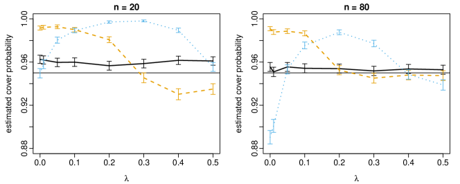
Figure 2: Monte Carlo estimates of coverage probabilities of confidence regions from inverting the modified score (solid), likelihood ratio (dashed), and Wald (dotted) test statistics. The straight horizontal line indicates the nominal 0.95 coverage probability and vertical bars denote $\pm 2$ times Monte Carlo standard errors.

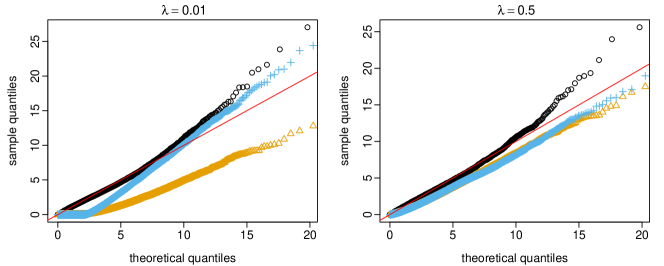
Figure 3: Quantile-quantile plots for modified score (circles), likelihood ratio (triangles), and Wald (plus signs) test statistics. The theoretical quantiles are from the chi-square distribution with 2 degrees of freedom and the sample quantiles from 10,000 Monte Carlo replications with $(n,r)=(80,10)$.

For additional insight into test statistics’ behavior near critical points, Figure 4 shows estimated rejection probabilities (size and power) for tests of the null hypothesis that $\lambda_{1}=\lambda_{2}=10^{-6}$. The data generating settings are the same as those used for Figure 2. The power curves are not directly comparable because, as was also shown in Figure 2, the different tests have different sizes. Nevertheless, the power curves behave similarly as the true $\lambda$ moves away from the null hypothesis value. This indicates the differences in coverage observed in Figure 2 is not in general due to how large the different confidence regions are.

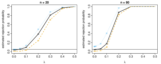
Figure 4: Monte Carlo estimates of rejection probabilities for testing the null hypothesis $\lambda=10^{-6}1_{2}$ using the modified score (solid), likelihood ratio (dashed), and Wald (dotted) test. The straight horizontal line indicates the size of the tests (0.05) and vertical bars denote $\pm 2$ times Monte Carlo standard errors.

We considered several configurations in addition to those reported, including both larger and smaller values of $n$ and $\lambda$, and the results were remarkably consistent. To compute the proposed test statistic, we used the lmmstest R package written by the first author. To fit the model and compute the likelihood ratio and Wald test statistics we used the lme4 R package (Bates et al.,, 2015). The Supplementary Material includes times for computing the test-statistics in the simulations on which Figure 2 is based. The proposed test-statistic was about 3–4 times faster to evaluate than the likelihood ratio and Wald statistics on average, but we expect both relative and absolute computing times to vary substantially between settings and implementations.

We also note there is a Stata routine for calculation of the proposed confidence region for a single variance parameter in linear mixed models with a random intercept (Bottai and Orsini,, 2004), a special case which can also be treated using exact finite sample methods (Crainiceanu and Ruppert,, 2004).

5 Data example

We illustrate using a dataset presented by Fitzmaurice et al., (2012) which contains a subset of the pulmonary function data collected in the Six Cities Study (Dockery et al.,, 1983). The data include a pulmonary measure called the forced expiratory volume in the first second (FEV1), height (ht), and age obtained from a randomly selected subset of the female participants living in Topeka, Kansas. The sample includes $n=300$ girls and young women, with a minimum of one and a maximum of twelve observations over time. Age and height are believed to be associated with the ability to take in and force out air. To model these data, consider the linear mixed model

$$\mathtt{FEV1}_{it}=\psi_{1}+\psi_{2}\mathtt{age}_{it}+\psi_{3}\mathtt{ht}_{it}+\psi_{4}\mathtt{age}_{i1}+\psi_{5}\mathtt{ht}_{i1}+U_{i1}+U_{i2}\mathtt{age}_{it}+E_{it},$$ (14)

where $U_{i1}\sim\mathcal{N}(0,\lambda_{1}^{2})$, $U_{i2}\sim\mathcal{N}(0,\lambda_{2}^{2})$, and $E_{it}\sim\mathcal{N}(0,\sigma^{2})$ are mutually independent for all individuals indexed by $i$ and time points indexed by $t$. This is a model considered by Fitzmaurice et al., (2012), modified slightly to fit our setting. The parameter set is $\Theta=\{\theta=(\psi,\lambda,\sigma)\in\mathbb{R}^{5}\times[0,\infty)^{2}\times(0,\infty)\}$.

Parameter	Estimate	Mod. Score CI	Lik. Rat. CI	Wald CI
$\lambda_{1}$ (intercept)	$0$	$(0,0.0482)$	$(0,0.0604)$	$(0,0.126)$
$\lambda_{2}$ (age)	$0.0201$	$(0.0188,0.0219)$	$(0.0183,0.0222)$	$(0.0181,0.0222)$
$\sigma$ (error)	$0.156$	$(0.152,0.162)$	$(0.151,0.162)$	$(0.151,0.162)$

Table 1: Maximum likelihood estimates and 95% confidence intervals (CI) for scale parameters in the linear mixed model (14).

The maximum likelihood estimate of $\psi$ is $\hat{\psi}=(-2.2,0.078,2.80,-0.040,-0.19)$, but we focus on the scale parameters whose estimates are in Table 1. Notably, the maximum likelihood estimate of $\lambda_{1}$ is zero, indicating common confidence regions may be unreliable. We present a confidence region for $\lambda$ (Figure 5) and three componentwise confidence regions (Table 1). When creating a confidence region for a sub-vector or component of $\theta$, say $\lambda_{1}$, the other components are effectively nuisance parameters. Then, at non-critical points we standardize the score for $\lambda_{1}$ by the Schur complement (efficient information) $\mathcal{I}_{n}/\mathcal{I}_{n}^{-\lambda_{1}}$, where $\mathcal{I}_{n}^{-\lambda_{1}}$ is $\mathcal{I}_{n}$ with rows and columns corresponding to $\lambda_{1}$ removed and evaluate at estimates of the nuisance parameters (see e.g. Fewster and Jupp, (2013) or Bickel et al., (1998, Chapter 2) for motivation). Similarly, at critical points we standardize the modified score for $\lambda_{1}$ by $\tilde{\mathcal{I}}_{n}/\tilde{\mathcal{I}}_{n}^{-\lambda_{1}}$; we comment further on nuisance parameters in Section 6.

For context, we also present likelihood ratio intervals based on the profile likelihood computed using the confint function in lme4, and Wald intervals based on maximum likelihood estimates from lme4 and the expected Fisher information evaluated at estimates. These use the chi-square distribution with one degree of freedom as reference. To decide whether to include the boundary points $\lambda_{1}=0$ and $\lambda_{2}=0$ in the componentwise confidence intervals, we note $\hat{\lambda}_{1}=0$ so $0$ is in confidence intervals based on the profile likelihood or Wald statistic for any reference distribution. Conversely, the test statistics for $\lambda_{2}$ are so large at $0$ that $0$ should not be in either region for any relevant reference distribution. To validate this, we used the varTestnlme R package (Baey and Kuhn,, 2019) to test, separately, $\lambda_{1}^{2}=0$ and $\lambda_{2}^{2}=0$, and got the $p$-values $0.5$ and $4\times 10^{-78}$, respectively.

The proposed interval for $\lambda_{1}$ is substantially smaller than that based on the likelihood ratio (Table 1). This is consistent with our simulations where the latter had greater than nominal empirical coverage of small scale parameters. The Wald interval for $\lambda_{1}$ is even wider than the likelihood ratio-based interval. The proposed interval for $\lambda_{2}$ is smaller than the other two, and its left endpoint is further from zero. Thus, there are indications the proposed procedure leads to not only reliable but more precise inference. The intervals for $\sigma$ only differ in the third significance digit. This is consistent with both theory and simulations since the estimate of $\sigma$ is further from zero than those of $\lambda_{1}$ and $\lambda_{2}$, and hence the different test statistics are expected to behave similarly.

Figure 5 shows plots of the componentwise test statistics based on the proposed method for a range of $\lambda_{1}$ and $\lambda_{2}$. The values of $\lambda_{1}$ and $\lambda_{2}$ such that the graph of the corresponding test statistic is below the critical value $3.84$, the $0.95$th quantile of the chi-square distribution with one degree of freedom, give the confidence regions in Table 1. The graphs indicate the test statistics are convex in $\lambda_{1}$ and $\lambda_{2}$, respectively. The proposed regions for $\lambda$ (Figure 5, third plot), which use the chi-square distribution with two degrees of freedom as reference distribution, can be used to assess which values of $\lambda$ are supported by the data. We may, for example, reject the joint null hypothesis that $\lambda_{1}=\lambda_{2}=0$ at conventional levels of significance. To create these graphs and the corresponding confidence regions in Table 1, we evaluated the test statistics at a grid of 50 values each for $\lambda_{1}$ and $\lambda_{2}$ and included in the confidence regions those points where the test-statistics were less than the desired quantile of the reference distributions. Thus, for the first and second plot we evaluated componentwise test-statistics 50 times each, and for the third plot we evaluated the test-statistic for $\lambda$ at $50\times 50=2500$ points. The coarseness of the grid can be adjusted depending on desired accuracy and computing times.

Figure 5: Componentwise test statistics for $\lambda_{1}$ (first plot) and $\lambda_{2}$ (second plot), and joint 80–99 % confidence regions for $\lambda$ (third plot), based on the chi-square distribution with two degrees of freedom. The dashed lines in the first two plots mark the 0.95th quantile of a chi-square distribution with one degree of freedom. The dashed lines in the third plot mark maximum likelihood estimates.

6 Final remarks

Linking the boundary problem to the singular information problem allows a deeper understanding of the behavior of the likelihood function in shrinking neighborhoods of the boundary of a parameter set. Perhaps more importantly, it permits the construction of confidence regions that have asymptotically correct uniform coverage probability.

The advantages of using the proposed modified score test in constructing confidence regions are many-fold: the proposed procedure does not in general require a consistent point estimator, which can be troublesome when the parameter is at or near the boundary; it does not in general rely on simulation algorithms, which typically need to be programmed for the specific problem at hand; it can be applied to a broad variety of models, including the linear mixed model; it allows inference on scale parameters when the random effects follow an asymmetric distribution, which gives insight about the sign and the magnitude of the skewness. In addition, to the best of our knowledge, the asymptotic behavior under a sequence of parameters of the Wald and likelihood ratio test statistics for a scale parameter, has not been described for settings in which the Fisher information has any rank less than full.

Our work suggests several avenues for future research: First, more theory is needed on settings with nuisance parameters not orthogonal to the parameters of interest. Existing theory suggests replacing the Fisher information by the efficient Fisher information as we did in Section 5, but this has not been formalized for inference near critical points. Based on simulations (Supplementary Material) and intuition, we conjecture our results may be adapted to settings where the block of the Fisher information corresponding to the nuisance parameters is not nearly singular, but that there may be additional challenges otherwise. Second, in some mixed models, for example with crossed random effects, there are few independent observations even as the total number of observations grows. Then, a different asymptotic theory may be of interest. There are results on the consistency of maximum likelihood estimators in such settings (Jiang,, 2013; Ekvall and Jones,, 2020), but the properties of test statistics are largely unknown. Third, efficient software implementations of the proposed method for popular mixed models are needed: creating the proposed confidence region in practice often requires inverting the test-statistic numerically which can be computationally expensive. This is in contrast to the Wald statistic which can be inverted analytically, but similarly to the likelihood ratio statistic which in general requires numerical inversion. A natural starting point when implementing a numerical procedure would be to consider a grid of parameter values centered at some reasonable estimates. For example, even in non-linear mixed models where maximum likelihood estimation can be computationally expensive, fast approximate maximum likelihood estimates and Wald confidence regions are often available through penalized quasi-likelihood or Laplace approximation of the likelihood. Some further remarks on computing are in the Supplementary Material.

References

- Azzalini and Capitanio, (2014) Azzalini, A. and Capitanio, A. (2014). The Skew-Normal and Related Families. Number 3 in Institute of Mathematical Statistics monographs. Cambridge University Press, Cambridge.
- Baey et al., (2019) Baey, C., Cournède, P.-H., and Kuhn, E. (2019). Asymptotic distribution of likelihood ratio test statistics for variance components in nonlinear mixed effects models. Computational Statistics & Data Analysis, 135:107–122.
- Baey and Kuhn, (2019) Baey, C. and Kuhn, E. (2019). varTestnlme: variance components testing in mixed-effect models.
- Bates et al., (2015) Bates, D., Mächler, M., Bolker, B., and Walker, S. (2015). Fitting linear mixed-effects models using lme4. Journal of Statistical Software, 67(1).
- Bhatia, (2012) Bhatia, R. (2012). Matrix Analysis. Springer New York.
- Bickel et al., (1998) Bickel, P. J., Klaassen, C. A. J., Ritov, Y., and Wellner, J. A. (1998). Efficient and Adaptive Estimation for Semiparametric Models. Springer-Verlag, New York.
- Billingsley, (1995) Billingsley, P. (1995). Probability and Measure. Wiley series in probability and mathematical statistics. Wiley, New York, 3rd ed edition.
- Billingsley, (1999) Billingsley, P. (1999). Convergence of Probability Measures. Wiley series in probability and statistics. Probability and statistics section. Wiley, New York, second edition.
- Biscio et al., (2018) Biscio, C. A. N., Poinas, A., and Waagepetersen, R. (2018). A note on gaps in proofs of central limit theorems. Statistics & Probability Letters, 135:7–10.
- Bottai, (2003) Bottai, M. (2003). Confidence regions when the Fisher information is zero. Biometrika, 90(1):73–84.
- Bottai and Orsini, (2004) Bottai, M. and Orsini, N. (2004). Confidence intervals for the variance component of random-effects linear models. The Stata Journal: Promoting communications on statistics and Stata, 4(4):429–435.
- Chen et al., (2019) Chen, S. T., Xiao, L., and Staicu, A.-M. (2019). An approximate restricted likelihood ratio test for variance components in generalized linear mixed models. arXiv:1906.03320 [stat].
- Chesher, (1984) Chesher, A. (1984). Testing for neglected heterogeneity. Econometrica, 52(4):865–872.
- Cox and Hinkley, (2000) Cox, D. R. and Hinkley, D. V. (2000). Theoretical Statistics. Chapman & Hall/CRC, Boca Raton.
- Crainiceanu and Ruppert, (2004) Crainiceanu, C. M. and Ruppert, D. (2004). Likelihood ratio tests in linear mixed models with one variance component. Journal of the Royal Statistical Society: Series B (Statistical Methodology), 66(1):165–185.
- Dockery et al., (1983) Dockery, D., Berkey, C., Ware, J., Speizer, F., and Ferris Jr, B. (1983). Distribution of forced vital capacity and forced expiratory volume in one second in children 6 to 11 years of age. American Review of Respiratory Disease, 128(3):405–412.
- Drikvandi et al., (2013) Drikvandi, R., Verbeke, G., Khodadadi, A., and Partovi Nia, V. (2013). Testing multiple variance components in linear mixed-effects models. Biostatistics, 14(1):144–159.
- Ekvall and Jones, (2020) Ekvall, K. O. and Jones, G. L. (2020). Consistent maximum likelihood estimation using subsets with applications to multivariate mixed models. Annals of Statistics, 48(2):932–952.
- Fewster and Jupp, (2013) Fewster, R. M. and Jupp, P. E. (2013). Information on parameters of interest decreases under transformations. Journal of Multivariate Analysis, 120:34–39.
- Fitzmaurice et al., (2012) Fitzmaurice, G. M., Laird, N. M., and Ware, J. H. (2012). Applied Longitudinal Analysis. John Wiley & Sons, Hoboken, NJ.
- Fitzmaurice et al., (2007) Fitzmaurice, G. M., Lipsitz, S. R., and Ibrahim, J. G. (2007). A note on permutation tests for variance components in multilevel generalized linear mixed models. Biometrics, 63(3):942–946.
- Folland, (2007) Folland, G. B. (2007). Real Analysis: Modern Techniques and Their Applications. Wiley, New York, second edition.
- Fristedt and Gray, (2013) Fristedt, B. E. and Gray, L. F. (2013). A Modern Approach to Probability Theory. Birkhäuser Boston, Boston, MA.
- Geyer, (1994) Geyer, C. J. (1994). On the asymptotics of constrained M-estimation. Annals of Statistics, 22(4):1993–2010.
- Giampaoli and Singer, (2009) Giampaoli, V. and Singer, J. M. (2009). Likelihood ratio tests for variance components in linear mixed models. Journal of Statistical Planning and Inference, 139(4):1435–1448.
- Greven et al., (2008) Greven, S., Crainiceanu, C. M., Küchenhoff, H., and Peters, A. (2008). Restricted likelihood ratio testing for zero variance components in linear mixed models. Journal of Computational and Graphical Statistics, 17(4):870–891.
- Hall and Praestgaard, (2001) Hall, D. B. and Praestgaard, J. T. (2001). Order-restricted score tests for homogeneity in generalised linear and nonlinear mixed models. Biometrika, 88(3):739–751.
- Jiang, (2013) Jiang, J. (2013). The subset argument and consistency of MLE in GLMM: Answer to an open problem and beyond. The Annals of Statistics, 41(1).
- Knudson et al., (2021) Knudson, C., Benson, S., Geyer, C., and Jones, G. (2021). Likelihood-based inference for generalized linear mixed models: Inference with the R package glmm. Stat, 10(1):e339.
- Lee and Chesher, (1986) Lee, L.-F. and Chesher, A. (1986). Specification testing when score test statistics are identically zero. Journal of Econometrics, 31(2):121–149.
- Lin, (1997) Lin, X. (1997). Variance component testing in generalised linear models with random effects. Biometrika, 84(2):309–326.
- McCulloch et al., (2008) McCulloch, C. E., Searle, S. R., and Neuhaus, J. M. (2008). Generalized, linear, and mixed models. John Wiley & Sons, Hoboken, NJ.
- Qu et al., (2013) Qu, L., Guennel, T., and Marshall, S. L. (2013). Linear score tests for variance components in linear mixed models and applications to genetic association studies: linear score tests for variance components. Biometrics, 69(4):883–892.
- Rotnitzky et al., (2000) Rotnitzky, A., Cox, D. R., Bottai, M., and Robins, J. (2000). Likelihood-based inference with singular information matrix. Bernoulli, 6(2):243–284.
- Saville and Herring, (2009) Saville, B. R. and Herring, A. H. (2009). Testing random effects in the linear mixed model using approximate Bayes factors. Biometrics, 65(2):369–376.
- Self and Liang, (1987) Self, S. G. and Liang, K.-Y. (1987). Asymptotic properties of maximum likelihood estimators and likelihood ratio tests under nonstandard conditions. Journal of the American Statistical Association, 82(398):605–610.
- Sinha, (2009) Sinha, S. K. (2009). Bootstrap tests for variance components in generalized linear mixed models. Canadian Journal of Statistics, 37(2):219–234.
- Stern and Welsh, (2000) Stern, S. E. and Welsh, A. H. (2000). Likelihood inference for small variance components. Canadian Journal of Statistics, 28(3):517–532.
- Stram and Lee, (1994) Stram, D. O. and Lee, J. W. (1994). Variance components testing in the longitudinal mixed effects model. Biometrics, 50(4):1171–1177.
- Stram and Lee, (1995) Stram, D. O. and Lee, J. W. (1995). Corrections: Variance component testing in the longitudinal mixed effects model. Biometrics, 51(3):1196.
- Verbeke and Molenberghs, (2003) Verbeke, G. and Molenberghs, G. (2003). The use of score tests for inference on variance components. Biometrics, 59(2):254–262.
- Wiencierz et al., (2011) Wiencierz, A., Greven, S., and Küchenhoff, H. (2011). Restricted likelihood ratio testing in linear mixed models with general error covariance structure. Electronic Journal of Statistics, 5(0):1718–1734.
- Wood, (2013) Wood, S. N. (2013). A simple test for random effects in regression models. Biometrika, 100(4):1005–1010.
- Zhu and Zhang, (2006) Zhu, H. and Zhang, H. (2006). Generalized score test of homogeneity for mixed effects models. The Annals of Statistics, 34(3):1545–1569.