A gravitational-wave perspective on neutron-star seismology

Abstract

We provide a bird’s-eye view of neutron-star seismology, which aims to probe the extreme physics associated with these objects, in the context of gravitational-wave astronomy. Focussing on the fundamental mode of oscillation, which is an efficient gravitational-wave emitter, we consider the seismology aspects of a number of astrophysically relevant scenarios, ranging from transients (like pulsar glitches and magnetar flares), to the dynamics of tides in inspiralling compact binaries and the eventual merged object and instabilities acting in isolated, rapidly rotating, neutron stars. The aim is not to provide a thorough review, but rather to introduce (some of) the key ideas and highlight issues that need further attention.

I Motivation

Neutron stars represent many extremes of physics; in density, pressure, temperature (through the early formation stages and during binary mergers), models for which require aspects that may not yet be fully (or perhaps even partially) understood. The composition and state of matter introduce concepts from across modern physics—fluid dynamics and elasticity, thermodynamics, superfluidity and superconductivity, electromagnetism, nuclear physics—while the models have to be developed in the curved spacetime framework of general relativity. To suggest that this is a challenge is not an understatement. In fact, from the theory point of view we may have to accept that we cannot—at least not at this point—account for all aspects we know we ought to consider. Then there are (in the words of a wise philosopher) the “unknown unknows”… Yet, we want to make progress.

The obvious question to ask is if we can use observations to make sense of the theory mess. This may seem far fetched, given that neutron stars are small and (obviously) distant. They are certainly not hands-on laboratories! Nevertheless, there has been clear progress. Notably, we have precise mass estimates for many systems from radio pulsar timing (telling us, in particular, that the matter equation of state must allow stars with a mass above $2M_{\odot}$ Demorest et al. (2010)) and the recent results from NICER constrain the neutron star radius (very roughly to the range 11-14 km), as well Riley et al. (2019); Miller et al. (2019). The constraints on bulk properties—mass and radius—should become increasingly precise as more data become available. Future instruments, like the SKA in the radio and the planned eXTP mission for x-ray timing Watts et al. (2016), will ensure that this remains a healthy area of exploration. What is less clear is to what extent this progress will allow us to probe aspects associated with the neutron star interior, e.g. the state and composition of matter.

If we want to explore aspects associated with the dense neutron star interior, it is natural to (try to) formulate a seismology strategy. It is well-known that the complex interior physics is reflected in a rich spectrum of oscillation modes Andersson (2019) and one may hope to be able to use observations of related features to gain insight. Similar observation programmes have been been carried out—with enormous success—for both the Sun and distant main-sequence stars. In the case of the Sun, much of the progress was driven by the ESA/NASA SOHO (SOlar and Heliospheric Observatory) space mission. Studies of gravity g-modes and low-multipole pressure p-modes have led to measures of the sound speed at different depths and the differential rotation throughout much of the Sun’s interior. For other stars, NASA’s Kepler mission has provided key information about the structure and internal dynamics, focussing on oscillations that are stochastically excited by surface convection. This has led to a revolution is the field of asteroseismology Aerts et al. (2010). Interestingly, the same technology allows us to characterise the host stars of exoplanets, as the inference of a precise stellar radius constrains the companion planetary radius, as well.

When it comes to neutron stars, we are not likely to be able to “resolve” surface features. Instead, it is natural to consider the gravitational-wave aspects of the problem. In essence, any non-axisymmetric deformation/acceleration of the matter in the star will generate gravitational waves and one would expect to be able to express these waves in terms of the star’s oscillation modes. The promise of such gravitational-wave asteroseismology Andersson and Kokkotas (1996, 1998); Kokkotas et al. (2001); Benhar et al. (2004) relies on the answer to two questions. First, are the mode features robust enough that we can use observations to constrain the physics? Second, are there realistic scenarios where specific oscillation modes are excited to a level that the gravitational-wave signal can be detected by current (or, indeed, future) instruments? Our aim here is to argue in favour of affirmative answers to both of these questions. This is not to say that this venture will be in any way straightforward, but the effort may pay off handsomely in the end.

II The first couple of steps: The f-mode

As a first illustration of the key aspects, let us consider the simplest setting; a non-rotating uniform density star. This problem was considered by Lord Kelvin back in the late 1800s, although the analysis was carried out in a fashion that would seem arcane to a modern student (as it did not involve spherical harmonics).

In Newtonian gravity, the dynamics of a non-rotating star is governed by the Euler equations (momentum conservation), together with the continuity equation (mass conservation) and the Poisson equation for the gravitational potential. As we are (for now) taking the density, $\rho$, to be constant, the continuity equation simplifies and we have (working in a coordinate basis so that $\nabla_{i}$ represents the covariant derivative associated with the chosen coordinates)

$$\partial_{t}\rho+\nabla_{i}(\rho v^{i})=0\Longrightarrow\nabla_{i}v^{i}=0\ .$$ (1)

That is, the fluid flow—represented by the velocity $v^{i}$—is incompressible. Analysing the problem, we need to distinguish two kinds of perturbations. Eulerian perturbations relate to changes in the various quantities at a fixed point in space; e.g. $\delta p$ for the pressure (where we obviously have $\delta\rho=0$ in this first example). This is in contrast to co-moving Lagrangian perturbations, which relate to measurements carried out by an observer moving along with the fluid. This leads to a pressure perturbation $\Delta p$ and if we introduce a displacement vector $\xi^{i}$ to connect the perturbed fluid elements with the corresponding ones in the unperturbed configuration, we have Friedman and Schutz (1978)

$$\Delta p=\delta p+\xi^{i}\nabla_{i}p\ .$$ (2)

For non-rotating stars, which we focus on for the moment, the displacement vector is simply related to the perturbed velocity through

$$\partial_{t}\xi^{i}=\Delta v^{i}=\delta v^{i}\ .$$ (3)

In terms of Eulerian pertubations, the momentum equation takes the form

$$\partial_{t}\delta v_{i}+{1\over\rho}\nabla_{i}\delta p+\nabla_{i}\delta\Phi=0\ ,$$ (4)

where $\delta\Phi$ is the variation in the gravitational potential, which is governed by

$$\nabla^{2}\delta\Phi=4\pi\delta\rho\ ,$$ (5)

such that the right-hand side vanishes for a constant density model. It follows immediately from these equations that the perturbed velocity must be irrotational and hence it makes sense to introduce a velocity potential such that

$$\delta v_{i}=\nabla_{i}\chi\ .$$ (6)

The perturbed Euler equations then lead to

$$\partial_{t}\chi+{1\over\rho}\delta p+\delta\Phi=\mbox{ constant}\ .$$ (7)

It follows that $\chi$, $\delta p$ and $\delta\Phi$ must all solve the homogeneous version of Laplace’s equation. This, in turn, tells us that the quantities are naturally expanded in spherical harmonics, $Y_{l}^{m}$, and it is easy to show that, in order for the behaviour to be regular at the centre, each quantity must be proportional to $r^{l}Y^{m}_{l}$ for a given $(l,m)$ multipole. Finally, at the surface of the star, a given oscillation mode must satisfy

$$\Delta p=\delta p+\xi^{r}\partial_{r}p=0\qquad\mbox{ at }r=R\ ,$$ (8)

while the matching to the external gravitational potential requires

$$\partial_{r}\delta\Phi+{l+1\over R}\delta\Phi=-4\pi G\rho\xi^{r}\ ,\quad\mbox{ at }r=R\ ,$$ (9)

(noting that the right-hand side does not vanish for a constant density model or, indeed, whenever the star’s surface is associated with a finite density, as it might be for a quark star). Working out the algebra (in the Fourier-domain, with a harmonic time dependence $e^{i\omega t}$ for all quantities), we find that we must have

$$\omega^{2}={8\pi G\rho\over 3}{l(l-1)\over 2l+1}\ .$$ (10)

For each value of $l$ we have two modes (associated with the two signs of the square root), known as the fundamental f-modes. The mode frequency scales with the (square root of the) average density of the star and increases with the multipole $l$ (the mode frequencies are the same for all values of $m$ in a non-rotating star). The first scaling suggests that it ought to be possible to use observations to constrain the physics of the star. Of course, we also see that the observation of a single mode-frequency would not be enough, as it would only constrain the average density. We need more information to untangle mass and radius.

Next, in order to estimate the rate at which gravitational-wave emission damps the f-mode we can use the standard post-Newtonian multipole formulas Andersson (2019). Focussing on a single mode and the contribution from the mass multipole (noting that, in the case of the uniform density model, the contribution comes from the star’s surface, where the density is formally discontinuous Detweiler (1975)) we find the damping timescale

$$\tau\sim\left({c^{2}R\over GM}\right)^{l+1}{R\over c}\ ,$$ (11)

where $M$ is the star’s mass, $G$ is Newton’s gravitational constant and $c$ is the speed of light.

What do we learn from this? Perhaps the most important insight is this: A given uniform density model is described by two parameters, which we can take to be the density and the radius. An observation of the mode frequency would provide the former and then the damping rate would help us infer the radius—as the scaling with the parameters is different. This is the main idea of gravitational-wave asteroseismology Andersson and Kokkotas (1996, 1998); Kokkotas et al. (2001); Benhar et al. (2004) and it prompts a number of follow-on questions.

How likely are we to be able to infer both the frequency and the damping rate from observations? The answer depends on the energy associated with the mode excitation, but it is generally clear that—since these modes are rapidly damped—the oscillation frequency is easier to pin down than the damping. As an illustration, consider the example from Andersson (2019) (which draws on the empirical relations from Kokkotas et al. (2001)) which shows that—for a typical f-mode with frequency $f=2.4$ kHz and damping time $\tau=0.1$ s, a galactic source at a distance of $10$ kpc and a fiducial detector with sensitivity (spectral noise density) $S_{n}^{1/2}=10^{-23}$ Hz^-1/2 at the mode frequency (roughly the level of advanced LIGO instruments during the O3 science run), we expect a signal-to-noise ratio (not to be confused with the matter density)

$$\rho_{\mathrm{n}}\approx 30\left({E\over 10^{-6}M_{\odot}c^{2}}\right)^{1/2}\ ,$$ (12)

where $E$ represents the energy channeled through the specific mode we consider. We see that, if the system radiates about $E=4\times 10^{-7}M_{\odot}c^{2}$ through this mode we would detect the signal with $\rho_{\mathrm{n}}\approx 10$. The relative error involved in the parameter estimation may be estimated by a Fischer matrix analysis Kokkotas et al. (2001). In the suggested example, this leads to

$${\delta f/f}\approx 1.3\times 10^{-3}/\rho_{\mathrm{n}}\ ,$$ (13)

and

$${\delta\tau/\tau}\approx 2/\rho_{\mathrm{n}}\ .$$ (14)

For a signal leading to $\rho_{\mathrm{n}}\approx 10$ we would accurately infer the mode frequency but the damping rate would only be known at the 20% level. If we want to extract both the frequency and the damping rate to (say) the 1% level, then we need a signal-to-noise ratio of at least 200. This would require the release of an energy of order $4\times 10^{-5}M_{\odot}c^{2}$, which—as we will discuss below—may be unrealistic.

This brings us to the astrophysics. Are there realistic scenarios where different oscillation modes are excited to a significant amplitude? We will consider some possibilities later. And finally, what about more realistic stellar models? Are the suggested scaling relations robust for a range of (say) compressible equations of state? On the one hand, we want this to be the case as the observable features should then be robust, as well. On the other hand, we need there to be differences, as the main aim of the exercise is to identify the underlying matter properties and this (obviously) means that we need to be able to tell the difference between different models.

The last point suggests that we need to consider more realistic implementations based on relativistic neutron star models. Naturally, this calculation is a bit more involved. First of all, we need to account for the compressibility of matter. This means that we have to generalise the form for the displacement vector. Instead of working with the gradient of a scalar potential, we now have

$$\xi^{i}={W(r)\over r}\nabla^{i}r+V(r)\nabla^{i}Y_{lm}\ ,$$ (15)

We also need to consider the density variations. These are linked to the pressure via the equation of state, and depend explicitly on the speed of sound, $c_{s}$, in the stellar fluid. For a barotropic model with $p=p(\rho)$, we have

$$c_{s}^{2}={dp\over d\rho}\quad\mbox{and}\quad\Delta p={p\Gamma_{1}\over\rho}\Delta\rho=c_{s}^{2}\Delta\rho\ .$$ (16)

Notably, the background equilibrium and the Lagrangian perturbations are described by “the same” equation of state in this case. As we will see later, this is not generally the case.

Working through the details, we now find (in addition to the f-mode) a set of higher frequency pressure p-modes. These depend directly on the compressibility of matter. Higher overtone p-modes have—for a given multipole $l$—increasingly high frequecies. The p-modes tend to be less efficient emitters of gravitational waves as they have radial nodes in the eigenfunctions which lead to cancellations in the mass multipole integral Andersson et al. (1995). Moreover, as the typical p-mode frequency lies above several kHz, these modes will be difficult to detect with ground-based instruments (as these tend to be designed with binary inspirals in mind, leading to a sensitivity sweet spot around 100 Hz).

What happens when we consider the problem in general relativity, as we know we must if we want to use a realistic matter description? Qualitatively, the problem is different because the modes become “quasi”-normal. In a live spacetime, they are determined from an asymptotic condition of purely outgoing gravitational waves. This means that they have complex frequencies, with the imaginary part representing the damping rate—we no longer have to resort to the multipole formula, but the mode solution is more complicated as the outgoing wave condition needs to be implemented with care Andersson et al. (1995); Leins et al. (1993); Glampedakis and Andersson (2003). Fortunately, there are a number of robust methods for dealing with this issue.

Focussing on the f-mode, the relativistic results largely bring out the expectations from the Newtonian calculation. The results from Andersson and Kokkotas (1996, 1998) demonstrate that the scalings from (10) and (11) work pretty well, leading to useful phenomenological relations for the frequency and the damping rate. This is not too surprising because, even though the microphysics associated with different equations of state may be different, the neutron star bulk properties are fairly robust. In fact, Lattimer and Prakash have pointed out Lattimer and Prakash (2001) that the old Tolman VII solution to the Einstein equations Tolman (1939), which takes as the starting point a quadratic density distribution, accords extremely well with the results for a wide range of “realistic” equations of state. This, in turn, suggests that we should not be too surprised if different neutron star properties turn out to be related by more or less “universal” relations Yagi and Yunes (2013).

Returning to the f-mode, the relativistic mode frequencies encode a dependence on the gravitational redshift—as the modes are “observed” at infinity. This suggests an additional dependence on the star’s compactness, $M/R$, and hence a more complicated parameter scaling. The results from Tsui and Leung (2005) show that a scaling in powers of the stellar compactness leads to a useful f-mode relation for a range of matter models. An even tighter relation is provided in Lau et al. (2010), based on working with $\eta=(M^{3}/I)^{1/2}$, where $I$ is the star’s moment of inertia, as the scaling parameter. These relations are accurate enough that a seismology strategy can be formulated for realistic neutron star models.

III Transients

For isolated neutron stars, one might envisage a number of scenarios that lead to transient gravitational-wave emission which may, in turn, be channeled through individal modes of oscillations. In fact, if the modes form a complete set (in the mathematical sense) then it should be possible to represent any given “initial data” as a mode-sum. This should be the case in Newtonian theory (although the problem is intricate for rotating stars Friedman and Schutz (1978)), but the modes are not expected to be complete in relativity. In essense, we consider the likely energy budget for different “explosive” phenomena and then, through a back-of-the-envelope argument, estimate the gravitational-wave amplitude. This is instructive, but the exercise comes with important caveats. In particular, an energy based argument that something is possible in principle does not in any way demonstrate that this happens in reality—a simple reflection of the fact that we need the energy to be associated with asymmetries in the fluid motion in order to lead to gravitational-wave emission (a spherical expansion/contraction simply won’t do!). The converse is, of course, true. If we can show that there is not enough energy available to excite a given mode to a relevant amplitude then the proposed scenario is unlikely to be of interest.

We can estimate the gravitational-wave strain $h$ from the standard flux formula Andersson (2019)

$${c^{3}\over 16\pi G}|\dot{h}|^{2}={1\over 4\pi d^{2}}\dot{E}\ ,$$ (17)

where $d$ is the distance to the source, and the dots represent time derivatives. In our case, we characterize a given event by the damping time $\tau$ and assume that the signal is monochromatic, with mode-frequency $f$. Then we use $\dot{E}\approx E/\tau$ and $\dot{h}\approx 2\pi fh$ to get

$$h\approx 4\times 10^{-23}\left({E\over 10^{-9}M_{\odot}c^{2}}\right)^{1/2}\left({\tau\over 0.1\mbox{ s}}\right)^{-1/2}\left({f\over 2\mbox{ kHz}}\right)^{-1}\left({d\over 10\mbox{ kpc}}\right)^{-1}\ ,$$ (18)

This rough estimate accords fairly well with the more precise statement of detectability from before. The key point is that, for the energy budget to be reasonable we have to focus on galactic events.

What kind of—ideally regularly occurring—astrophysical event may lead to a neutron star exhibiting “large” amplitude oscillations? The traditional example would be the supernova explosion in which the star is born. However, estimates for the energy radiated as gravitational waves from supernovae tend to be rather pessimistic, suggesting a total release of no more than the equivalent to $10^{-6}M_{\odot}c^{2}$, or so. This might still be enough to secure a detection, but as we only expect a few galactic supernovae per century we may need a fair bit of patience. Nevertheless, recent work has demonstrated that there are interesting seismology aspects to the core collapse problem Burrows et al. (2006); Radice et al. , so it is clearly worth pursuing this in more detail.

Another potential excitation mechanism for stellar oscillations would be some kind of starquake, e.g., associated with a pulsar glitch or a magnetar flare. The idea is that the evolution of the star—e.g. associated with magnetic field decay— leads to strain in the elastic crust and that the stored energy is suddenly released when the system reaches a critical level. The typical energy released in this process would then be of the order of the maximum mechanical energy that can be stored in the crust, estimated to be at the level of $10^{-9}-10^{-7}M_{\odot}c^{2}$ Blaes et al. (1989); Mock and Joss (1998). This suggestion is interesting given that magnetars appear to be associated with fairly regular flaring events Watts et al. (2016). If modes are excited in these systems, an indication of the energy released in the most powerful bursts is the $10^{-9}M_{\odot}c^{2}$ estimated for the March 5 1979 burst in SGR 0526-66 Barat et al. (1983). However, if the main action leading to the energy emission is associated with the low-density crust one would not expect significant gravitational-wave emission. We may use observations as basis for an asteroseismology analysis—as has indeed be done Samuelsson and Andersson (2007)—but the gravitational-wave aspect would be missing. This does not means that we should not search for counterpart signals to the observed flares—as has, indeed, been done Baggio et al. (2005); Abbott et al. (2007, 2008, 2009); Abadie et al. (2011)—but we should do this with realistic expectations.

The situation is somewhat similar for pulsar glitches, although these events involve significantly less energy. In this case the release of energy is assumed to be associated with large-scale superfluid vortex unpinning in the outer core/inner crust of the star Haskell and Melatos (2015). A simple energy estimate suggests that these events may be interesting for the dedicated gravitational-wave astronomer Andersson and Comer (2001), but a closer analysis indicates that the excitation of the large-scale fluid motion we require may be less likely Sidery et al. (2010). Still, searches for glitch-related transients in LIGO gravitational-wave data have already been carried out 2011PhRvD..83d2001A .

Yet another scenario associated with the star’s evolution relates to internal phase transitions. The idea is simple. As the star spins down—due to the expected electromagnetic braking torque—the centrifugal force decreases and the star’s central density increases. If the equation of state predicts a sharp phase transition at some density, e.g. linked to quark deconfinement, then the star might rapidly contract when this density is reached. This contraction leads to potential energy being converted into heat and, perhaps, gravitational waves, as well. The latter component may, however, be small unless one can think of a way for the phase transition to induce asymmetries. At the end of the day, the different evolutionary scenarios are perfectly reasonable, but—in each case—it is difficult to predict the actual level of gravitational-wave emission. From the theory point of view this is problematic, but this does not mean that observers should not look for this kind of signal. Perhaps we need an observational breakthrough to get the theory right.

Another issue with transient events is that one would have to distinguish an astrophysical signal from instrumental artefacts; something that goes “ping” in the detector. Both may look like exponentially damped sinusoids, so how do we tell the difference? In this respect, it is interesting to note the transient candidate S191110af, announced by the LIGO/Virgo collaboration on November 10 2019. The suggested “signal” consisted of a 1.78 kHz oscillation lasting 0.104 s Chatterjee (2019a). Follow-up analysis identified instrumental artefacts in the data, which led to retraction of S191110af as a genuine signal Chatterjee (2019b). However, in the intervening time it was noted that the parameters were consistent with the f-mode of a fairly typical neutron star, see Kaplan and Read (2019) and the simple estimates from above. It was also noted that there was no evidence that a glitching pulsar could be responsible for S191110af Kaplan and Read (2019). The incidence is nevertheless interesting. The key point is that, while the particular event is unlikely to have been of astrophysical origin, we have seen that neutron stars can exhibit transients at the required level. Hence, it is natural to ask if we can design a strategy that makes a distinction between astrophysical transients and instrumental features. An interesting suggestion in this direction is outlined in Ho et al. (2020). The idea is to bring in additional information. First of all, a transient associated with (say) an f-mode oscillation would have to correlate with both the frequency and the damping rate. However, we know from the example of S191110af that this may not be enough. In the ideal case we would have an electromagnetic counterpart signal—a gamma-ray flare, an x-ray feature or perhaps a radio pulsar glitch—but one might have to be very lucky to make such an observation. Another reasonable strategy would be to draw on the known neutron star population. Is there for example an excess of transients with “neutron star-like” features and an energy distribution such that is could reasonably be associated with the galactic neutron star population? The argument then becomes statistical rather than based on a single outstanding event. This raises other issues, but it is one direction in which we might be able to make progress.

IV Adding physics: The g-modes

So far we have not considered the complex physics that characterises the neutron star interior. Additional features come into play when we consider the matter description beyond the pressure-density relation; when we account for the composition and state of matter. As a simple rule-of-thumb, each additional piece of “physics” brings (at least) one new class of oscillation modes into existence. This makes the seismology problem richer, but also more complicated as we need to keep track of new parameters and these may not be well constrained by our understanding of the nuclear physics. The pessimist may see an insurmountable obstacle here, but the optimist cannot help being excited by the discovery potential.

If we add internal stratification associated with, for example, temperature or composition gradients (like a varying proton fraction), then the so-called gravity g-modes come into play Reisenegger and Goldreich (1992). One immediate way of seeing this is to introduce the adiabatic index of the perturbations, $\Gamma_{1}$, as before;

$${\Delta p\over p}=\Gamma_{1}{\Delta\rho\over\rho}\ ,$$ (19)

leading to (for a spherical background star)

$$\delta p={p\Gamma_{1}\over\rho}\delta\rho+\xi^{i}\left[{p\Gamma_{1}\over\rho}\nabla_{i}\rho-\nabla_{i}p\right]\equiv{p\Gamma_{1}\over\rho}\delta\rho+p\Gamma_{1}({\xi^{r}}A)\ ,$$ (20)

which defines the Schwarzschild discriminant $A$. This adds a restoring force (buoyancy) for the perturbed fluid and leads to the presence of g-modes.

It is crucial to consider the impact of nuclear reactions on the composition g-modes. Following Andersson and Pnigouras we take as our starting point a two-parameter equation of state $p=p(\rho,x_{\rm p})$, where $x_{\rm p}=n_{\rm p}/n$ is the proton fraction (in terms of the proton and baryon number densities, $n_{\rm p}$ and $n$), and work in the context of Newtonian gravity. Then the mass density is simply $\rho=m_{B}n$ where $m_{B}$ is the baryon mass. In essence, we can think of $\rho$ as a proxy for the baryon number density, which is conserved (by virtue of the continuity equation). In order to account for nuclear reactions, we introduce a new dependent variable $\beta=\mu_{\rm n}-\mu_{\rm p}-\mu_{\rm e}$ which encodes the deviation from chemical equilibrium (with $\mu_{\mathrm{x}}$ and ${\mathrm{x}}={\rm n},{\rm p},{\rm e}$ representing the chemical potential for neutrons, protons and electrons, respectively). For simplicity, we assume a pure npe-matter neutron star core, which means that the relevant reaction timescales are those associated with the Urca reactions. Formally, we then have the thermodynamical relation (as we focus on the matter composition, we ignore the temperature here)

$$dp=\sum_{\mathrm{x}}n_{\mathrm{x}}d\mu_{\mathrm{x}}=n(d\mu_{\rm n}-x_{\rm p}d\beta)\ ,$$ (21)

where we have assumed (local) charge neutrality ($n_{\rm p}=n_{\rm e}$). As the background configuration is in both hydrostatic and beta equilibrium we only account for reactions at the level of the perturbations. We then, first of all, note that (21) should also hold for Lagrangian perturbations, so we have

$$\Delta p=n(\Delta\mu_{\rm n}-x_{\rm p}\Delta\beta)\ ,$$ (22)

or, as it turns out to be more convenient to work with $\rho$ and $\beta$,

$$\Delta p=\left({\partial p\over\partial\rho}\right)_{\beta}\Delta\rho+\left({\partial p\over\partial\beta}\right)_{\rho}\Delta\beta=c_{s}^{2}\Delta\rho+\left({\partial p\over\partial\beta}\right)_{\rho}\Delta\beta\ ,$$ (23)

where $c_{s}$ is sound speed for the background equilibrium.

How do we account for nuclear reactions? Well, for the protons we then have

$$(\partial_{t}+v^{j}\nabla_{j})n_{\rm p}+n_{\rm p}\nabla_{j}v^{j}=\Gamma\ ,$$ (24)

with $\Gamma$ the relevant reaction rate (not to be confused with the adiabatic index $\Gamma_{1}$). Combining this with overall baryon number conservation (assuming that all components move together!) and assuming that the reaction rate relates to perturbations, we have

$$\Delta\left[(\partial_{t}+v^{j}\nabla_{j})x_{\rm p}\right]=(\partial_{t}+v^{j}\nabla_{j})\Delta x_{\rm p}={\Gamma\over n}\ ,$$ (25)

where, at least for small deviations from equilibrium Haensel (1992); Reisenegger (1995),

$$\Gamma\approx\gamma\Delta\beta\ ,$$ (26)

with $\gamma$ encoding the relevant reaction rate.

Now thinking of $\beta$ as a function of $\rho$ and $x_{\rm p}$, and assuming that the star is non-rotating (so that $v^{i}=0$), we have

$$\partial_{t}\Delta\beta=\left({\partial\beta\over\partial\rho}\right)_{x_{\rm p}}\partial_{t}\Delta\rho+\left({\partial\beta\over\partial x_{\rm p}}\right)_{\rho}\partial_{t}\Delta x_{\rm p}=\left({\partial\beta\over\partial\rho}\right)_{x_{\rm p}}\partial_{t}\Delta\rho+\left({\partial\beta\over\partial x_{\rm p}}\right)_{\rho}{\gamma\over n}\Delta\beta\ .$$ (27)

That is, we have

$$\partial_{t}\Delta\beta-\mathcal{A}\Delta\beta=\mathcal{B}\partial_{t}\Delta\rho\ ,$$ (28)

with

$$\mathcal{A}=\left({\partial\beta\over\partial x_{\rm p}}\right)_{\rho}{\gamma\over n}\ ,\quad\mbox{and}\quad\mathcal{B}=\left({\partial\beta\over\partial\rho}\right)_{x_{\rm p}}\ .$$ (29)

If we work in the frequency domain (essentially assuming a time-dependence $e^{i\omega t}$ for the perturbations, and taking the coefficients $\mathcal{A}$ and $\mathcal{B}$ to be time independent) we have

$$\Delta\beta={\mathcal{B}\over 1+i\mathcal{A}/\omega}\Delta\rho\ .$$ (30)

At this point we can consider the timescales involved in the problem. Introducing a characteristic reaction time as

$$t_{R}={1\over\mathcal{A}}\ ,$$ (31)

(noting that the actual timescale is the absolute value of this) we see that, if the reactions are fast compared to the dynamics (associated with a timescale $\sim 1/\omega$) then $|t_{R}\omega|\ll 1$ and it follows that

$$\Delta\beta\approx 0\ .$$ (32)

Basically, because the dynamics are slow compared to the reactions the fluid remains in beta equilibrium. There will be no buoyancy and hence no g-modes. The situation changes in the limit of slow reactions, where $|t_{R}\omega|\gg 1$ and we can Taylor expand (30) to get

$$\Delta\beta\approx\mathcal{B}\left(1-i\mathcal{A}/\omega\right)\Delta\rho\approx\mathcal{B}\Delta\rho\ .$$ (33)

Using this result in (23), we have

$$\Delta p=\left[\left({\partial p\over\partial\rho}\right)_{\beta}+\left({\partial p\over\partial\beta}\right)_{\rho}\left({\partial\beta\over\partial\rho}\right)_{x_{\rm p}}\right]\Delta\rho\equiv\mathcal{C}\Delta\rho\ ,$$ (34)

which leads to

$$\delta p=\mathcal{C}\delta\rho+\left[\mathcal{C}\xi^{j}\nabla_{j}\rho-\xi^{j}\nabla_{j}p\right]\ .$$ (35)

with $\mathcal{C}=p\Gamma_{1}/\rho$. However, since

$$\nabla_{j}p=\left({\partial p\over\partial\rho}\right)_{\beta}\nabla_{j}\rho=c_{s}^{2}\nabla_{j}\rho\ ,$$ (36)

we are left with

$$\delta p=\mathcal{C}\delta\rho+\left({\partial p\over\partial\beta}\right)_{\rho}\left({\partial\beta\over\partial\rho}\right)_{x_{\rm p}}\xi^{j}\nabla_{j}\rho\ .$$ (37)

In this case, the composition of matter affects both terms on the right-hand side of the relation. The mathematics may be fairly straightforward, but the physics is less so. In particular, we now need an equation of state that allows us to calculate the different thermodynamical derivatives used to relate (37) and (20). While there are several such models “on the market” (a notable example being the results from the Brussels-Montreal collaboration Chamel et al. (2011)) it is clear that we are asking questions that go beyond the description of equilibrium configurations—we are beginning to touch upon issues like the relevant transport properties associated with the matter Schmitt and Shternin (2018).

This, fairly lengthy, argument may seem like a detour but it is important as it helps us understand a number of issues. First of all, we see that it is straightforward to analyse the problem in the two limits of fast and slow reactions. In the intermediate regime, where the dynamical timescale is similar to that of reactions we have to explicitly solve for the evolving proton fraction. Secondly, we see that the presence of g-modes depend entirely on the timescales. For example, the relatively slow Urca reactions (we will quantify this later) will allow g-modes associated with a varying proton fraction Reisenegger and Goldreich (1992), but as the relevant reactions are much faster there may be no g-modes arising from a varying hyperon fraction. Detailed mode calculations—ignoring the argument we have just outlined—suggest that the g-mode spectrum has a infinite number of “overtones” with decreasing frequency. Our argument obviously impacts on this. If we account for the reaction rates, then no matter how slow they are, there has to be a point where the oscillation of a (perhaps very) high order g-mode is even slower. This mode should not exist, at least not as an oscillation feature Andersson and Pnigouras . In essence, the spectrum of composition g-modes will actually be finite for a realistic neutron star model. The may seem like a fine-print issue, but it could be conceptually important (as in the tidal problem we consider below).

It is easy to see that thermal gradients may also lead to the presence of g-modes. The previous logic applies. We need the dynamics to be fast compared to the thermal evolution. Thermally supported g-modes are expected to be relevant for proto-neutron stars Ferrari et al. (2003); Gualtieri et al. (2004). The state of matter also affects the g-modes. For example, in a superfluid neutron star core—which requires a two-fluid model Andersson (2021)—the varying proton fraction will not introduce buyoancy. The g-modes disappear Lee (1995); Andersson and Comer (2001), at least until we reach the density where muons enter the game. At this point there will be a composition gradient, now associated with variations in the muon fraction. This re-introduces the g-modes, but at a slightly higher frequency (roughly a factor $1/x_{\rm p}$ higher than in the case of npe-matter) Gusakov and Kantor (2013); Passamonti et al. (2016).

V Dynamical tides

When we outlined scenarios for transient mode excitation we considered different mechanisms internal to the star. One may also envisage oscillations being driven by an external agent. The natural example of this is the tidal interaction in a binary system. When the two components of a binary system are far apart, a point-particle description of each body is sufficient to describe the orbital motion. This assumption is adequate for both classic binary dynamics and the post-Newtonian approximation used to model gravitational-wave signals from compact binaries Blanchet (2006). However, the situation changes as the stars are brought closer together through the emission of gravitational waves. Finite size effects come into play during the late stages of inspiral, with the tidal deformability Flanagan and Hinderer (2008); Hinderer (2008); Hinderer et al. (2010) of the supranuclear density matter,

$$\Lambda_{l}={2\over(2l-1)!!}{k_{l}\over\mathcal{C}^{2l+1}}\ ,$$ (38)

where $k_{l}$ is the Love number for the $l$-multipole and $\mathcal{C}=M/R$ is the stellar compactness, leaving an imprint on the gravitational-wave signal. As demonstrated in the celebrated case of GW170817—the first observed neutron star binary merger Abbott et al. (2017, 2018)—this leads to a constraint on the neutron star radius 2018PhRvL.121p1101A ; De et al. (2018) and hence the equation of state.

As it turns out, a precise understanding of the tidal response requires an analysis of both the state and composition of matter. One aspect of this relates to the composition of matter, which is likely to remain “frozen” during the late stages of binary inspiral. It is easy to see that this should be the case. A typical neutron star binary system may spend 10-15 minutes in the sensitivity band of a ground-based interferometer (above 10 Hz). As the stars are deformed by the tidal interaction, matter is driven out of equilibrium but the relevant nuclear reactions are (likely to be) too slow to re-establish equilibrium on this timescale. This is evident from, for example, the estimates in Haensel (1992), which suggest that the equilibration timescale for the direct Urca reactions is

$$t_{D}\sim 0.1~{}\mathrm{month}\left({T\over 10^{8}~{}\mathrm{K}}\right)^{-4}\ ,$$ (39)

with the modified Urca relaxation a factor of about $10^{7}$ slower (at $10^{8}$ K). Given that inspiralling binaries are mature—and hence cold—we can safely assume that the equilibration time will be much longer than the time it takes a given system to move through the sensitivity band of a ground-based interferometer (months-years vs minutes). In fact, at the expected core temperature the star’s interior should be superfluid, in which case reactions are suppressed (exponentially), see Yu and Weinberg (2017) for comments on how superfluidity impacts on the tidal problem (a problem with a number of interesting aspects). In essence, the equilibration argument supports the assumption that the equation of state is no longer barotropic, as has (indeed) been assumed in virtually every analysis of the tidal problem (see for example Lai (1994); Reisenegger and Goldreich (1994); Kokkotas and Schäfer (1995); Ho and Lai (1999)).

There are two main aspects to the tidal problem. First of all, the tidal deformability, usually represented by the Love numbers Flanagan and Hinderer (2008); Hinderer (2008); Hinderer et al. (2010), provide the static response during an adiabatic inspiral. Secondly, individual oscillation modes may become resonant with the tidal driving, leading to a distinct contribution for some specific frequency range. The two aspects may be explored separately (e.g. static deformations vs time-dependent ones) but as they are related it is useful to consider them within the same framework.

In the tidal case, the perturbed Euler equation (for a non-rotating and compressible star) is

$$\partial_{t}^{2}\xi_{i}+{1\over\rho}\nabla_{i}\delta p-{1\over\rho^{2}}\delta\rho\nabla_{i}p+\nabla_{i}\delta\Phi=-\nabla_{i}\chi$$ (40)

alongside the usual continuity equation and the Poisson equation for the gravitational potential. We also need the tidal potential $\chi$ (due to the presence of the binary partner), which is given by a solution to $\nabla^{2}\chi=0$. In a coordinate system centred on the primary, which we will take to have mass $M$, we have Ho and Lai (1999)

$$\chi=-GM^{\prime}\sum_{l\geq 2}\sum_{m=-l}^{l}{W_{lm}r^{l}\over D^{l+1}(t)}Y_{lm}e^{-im\psi(t)}\ ,$$ (41)

where $M^{\prime}$ is the mass of the secondary and $D$ is the orbital separation. The orbit of the companion is taken to be in the equatorial plane and $\psi$ is the orbital phase. For $l=2$ (which dominates the gravitational-wave contribution) we have

$$W_{20}=-\sqrt{\pi/5}\ ,\quad W_{2\pm 1}=0\ ,\quad W_{2\pm 2}=\sqrt{3\pi/10}\ .$$ (42)

We now want to express the driven response of the stellar fluid in terms of the (presumably complete ) set of normal modes. These correspond to solutions $\xi_{n}$ (where $n$ labels the different modes in a suitable way). Working in the frequency domain, i.e. solving the Fourier transform version of (40), and letting the mode-frequency be $\omega_{n}$ (real-valued in absence of dissipation) we have the mode-sum:

$$\xi^{i}=\sum_{n}a_{n}\xi_{n}^{i}\ ,$$ (43)

where each individual mode satisfies

$$-\omega_{n}^{2}A\xi_{n}^{i}+C\xi_{n}^{i}=0\ .$$ (44)

Here $A=\rho$, while the $C$ operator is messy but we do not need the explicit expression in the following. We will, however, make use of the orthogonality of the (time-independent) eigenfunctions. This is demonstrated by introducing the inner product from Friedman and Schutz (1978). For two solutions $\eta^{i}$ and $\xi^{i}$ to (44), we define

$$\langle\eta^{i},\xi_{i}\rangle=\int(\eta^{i})^{*}\xi_{i}dV\ ,$$ (45)

where the asterisk denotes complex conjugation. It follows that (suppressing the component indices to avoid cluttering up the expressions)

$$\left<\eta,A\xi\right>=\left<\xi,A\eta\right>^{*}\ \ ,$$ (46)

and

$$\left<\eta,C\xi\right>=\left<\xi,C\eta\right>^{*}\ .$$ (47)

From these symmetry relations it is relatively easy to show that two mode solutions $\xi^{i}_{n}$ and $\xi^{i}_{n^{\prime}}$ are orthogonal as long as $n\neq n^{\prime}$. That is, we have (keeping the normalisation of the modes explicit)

$$\langle\xi_{n^{\prime}},\rho\xi_{n}\rangle=\mathcal{A}_{n}^{2}\delta_{nn^{\prime}}\ ,$$ (48)

where (15) leads to (for polar modes, like the f-mode)

$$\mathcal{A}_{n}^{2}=\int_{0}^{R}\rho\left[W_{n}^{2}+l(l+1)V_{n}^{2}\right]dr\ .$$ (49)

We can also use the orthogonality to rewrite (40) as an equation for the mode amplitudes:

$$\ddot{a}_{n}+\omega_{n}^{2}a_{n}=-{1\over\mathcal{A}_{n}^{2}}\langle\xi_{n},\rho\nabla\chi\rangle\ .$$ (50)

Making use of the continuity equation and integrating by parts we have (assuming that the density vanishes at the surface of the star)

$$-\langle\xi_{n},\rho\nabla\chi\rangle=-\int\rho(\xi^{i}_{n})^{*}\nabla_{i}\chi dV=\int\chi\nabla_{i}(\rho\xi^{i}_{n})^{*}dV=-\int\chi\delta\rho^{*}_{n}dV\ .$$ (51)

Given the harmonic time dependence associated with the Fourier domain ($\sim e^{i\omega t}$) we have an equation for the amplitude of tidally driven modes (for each $l$, as the different values of $m$ are degenerate for non-rotating stars):

$$a_{n}={1\over\omega_{n}^{2}-\omega^{2}}{Q_{n}\over\mathcal{A}_{n}^{2}}v_{l}\ ,$$ (52)

where $v_{l}$ follows from (41) (after integrating out the angles) and we have introduced the “overlap integral”

$$Q_{n}=-\int\delta\rho^{*}_{n}r^{l+2}dr\ .$$ (53)

Noting that the frequency support of the tidal potential (for slowly evolving orbits) leads to $\omega=m\Omega$, where $\Omega$ is the orbital frequency, we have a driven set of modes which may become resonant during a binary inspiral Lai (1994); Reisenegger and Goldreich (1994); Kokkotas and Schäfer (1995).

The Poisson equation allows us to relate the density perturbation to the gravitational potential. The matching at the star’s surface then relates the result to the relevant multipole moments, and we have

$$Q_{n}={2l+1\over 4\pi G}R^{l+1}\delta\Phi_{n}(R)=I_{n}\ ,$$ (54)

where $I_{n}$ is the contribution each mode makes to the mass multipole moment. We can then quantify, for example, how much energy is deposited in a given mode during an inspiral. We can also express the result for the dynamical tide as an effective tidal deformability/Love number. The result we want follows immediately from

$$k_{l}={1\over 2}{\delta\Phi(R)\over\chi(R)}\ .$$ (55)

Expressed as a sum over the modes of the star Andersson and Pnigouras (2020), we have

$$k_{l}^{\mathrm{eff}}=-{1\over 2}+{1\over 2R^{l}}\sum_{n}{Q_{n}\over\mathcal{A}_{n}^{2}}{1\over\omega_{n}^{2}-(m\Omega)^{2}}\left[\omega^{2}V_{n}(R)-{GM\over R^{3}}W_{n}(R)\right]\ .$$ (56)

This provides us with a useful expression for the dynamical tide, calculable once we solve for star’s oscillation modes. Basically, the tidal response is a seismology problem Pratten et al. (2020); Andersson and Pnigouras (2021).

In addition to the dynamical tide, the mode-sum provides a representation for the static tide. In the low-frequency driving limit ($\Omega\to 0$) we retain the usual Love number. The relation is exact for the constant density model, where we only have to consider the f-mode. We then get Andersson and Pnigouras (2020)

$$k_{l}^{\mathrm{eff}}={\omega_{n}^{2}-GMl/R^{3}\over 2\left[(m\Omega)^{2}-\omega_{n}^{2}\right]}\to{3\over 4(l-1)}=k_{l}\quad\mbox{for}\ m\Omega\ll\omega_{n}\ .$$ (57)

This is the expected result for the Love number Poisson and Will (2014).

In general, the mode-sum allows us to quantify the level at which the matter composition enters the problem. Evidence for simple model problems (with a fixed value for $\Gamma_{1}$ providing the stratification) shows that the f-modes vastly dominate the tidal response, with p- and g-modes contributing at (most at) the few percent level Andersson and Pnigouras (2020). This is an interesting observation given that third generation (3G) gravitational-wave detectors like the Einstein Telescope or the Cosmic Explorer may be able to constrain the tidal deformability to the few percent level Martynov et al. (2016). It would certainly seem warranted to ask if this could allow us to use observations to constrain (some aspects of) the internal composition.

The mode sum allows us to make progress on a number of issues. For example, assuming that the f-mode dominates the mode sum—which seems a safe bet—it is easy to understand why we should expect to find a robust “universal relation” between the mode frequency and the tidal deformability. This result was demonstrated in Chan et al. (2014) and recent evidence suggests that the relation remains accurate for a wide range of equation of state models. Given this observation, we can combine the mode sum with the phenomenological relation from Chan et al. (2014) to write down—adding assumptions about the red shift of the frequencies involved—a similar phenomenological expression for the dynamical tide. As outlined in Andersson and Pnigouras (2021), this leads to

$$k_{l}^{\mathrm{eff}}\approx{\bar{\omega}_{f}^{2}k_{l}\over\bar{\omega}_{f}^{2}-\delta(2\bar{\Omega})^{2}}+{(2\bar{\Omega})^{2}\over\bar{\omega}_{f}^{2}-\delta(2\bar{\Omega})^{2}}\left[{\delta\over 2}-{\bar{\omega}_{f}^{2}\over\mathcal{C}^{3}}{\epsilon\over l}\left(k_{l}+{1\over 2}\right)\right]\ ,$$ (58)

where $\bar{\omega}_{f}=\omega_{f}M$ is the f-mode frequency ( the scaling with the star’s mass leading to the natural dimensionless combination in relativity, and the orbital frequency is scaled in the same way). As before, $k_{l}$ is the static Love number and we have introduced two free parameters, $\delta$ and $\epsilon$. The first of these, $\delta$, accounts for the gravitational redshift and the rotational frame-dragging induced by the orbital motion. However, it turns out that simply “removing” the redshift from the calculated mode frequency Steinhoff et al. (2016) by taking $\delta=1-2\mathcal{C}$ works quite well, so we are left with a one-parameter expression for the dynamical tide. The example in figure 1 shows that the result compares well with a more thorough analysis in the effective-one-body framework Hinderer et al. (2016); Steinhoff et al. (2016). Moreover, the dynamical tide has been shown to compare well with results extracted from numerical simulations Foucart et al. (2019). This suggests that we have a good understanding of the physics of the dynamical tide.

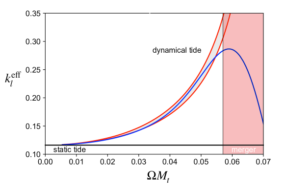
Figure 1: Comparing the effective Love number $k_{l}^{\mathrm{eff}}$ from (58), using $\delta=1-2\mathcal{C}$, to the results from Steinhoff et al. (2016) for the quadrupole ($l=2$) contribution to the dynamical tide. The horizontal line represents the static Love number ($k_{l}=k_{l}^{\mathrm{eff}}$ in the $\Omega\to 0$ limit). The result from Steinhoff et al. (2016) is shown as a solid blue curve, while estimates from (58) are shown for the range $\epsilon=0.85-0.9$ with the latter representing the lower edge of the filled (grey) band. The region beyond the merger frequency, $\Omega M_{t}\approx 0.057$, with $M_{t}$ the total mass of the binary, is indicated by the shaded region.

Finally, we can make contact with the end point of the binary evolution, the merger. The merger is associated with a wildly oscillating, hot remnant that (likely) eventually collapses to form a black hole. Interestingly (given the present context), numerical simulations demonstrate that the dynamics of the merged object exhibits robust high-frequency features Bauswein et al. (2014); Takami et al. (2014); Clark et al. (2016). These are generally thought to be associated with specific modes of oscillation, with the main feature associated with the fundamental mode Bauswein et al. (2016); Clark et al. (2016); Bernuzzi et al. (2015). This would be natural, although not straightforward to demonstrate as we have to explore perturbations relative to a background that evolves on a relatively short timescale.

From a seismology point of view, there is no reason to expect the merger dynamics to be connected with the inspiral phase. The physics of the equation of state should be “the same”, but the two inpiralling objects are cold (on the nuclear physics temperature scale) while the merged object is hot (possibly reaching temperatures higher than that of a supernova core) and differentially rotating. Since the thermal pressure and the rotation will both impact on the dynamics of the object Chakravarti and Andersson (2020) one would not expect features of the two stages to be related in a simple way. Nevertheless, they seem to be. Focussing on an equal-mass binary and introducing Bernuzzi et al. (2015)

$$\kappa_{2}^{t}=\frac{1}{8}\frac{k_{2}}{C^{5}}={3\over 16}\Lambda_{2}\ ,$$ (59)

one finds (empirically) that the main peak in the spectrum the merger dynamics ($f_{2}$) scales as

$$f_{2}M_{t}\approx 0.144(\kappa_{2}^{t})^{-0.278},$$ (60)

where $M_{t}$ is the total mass of the system (as before; here assuming that we can neglect mass ejected during the merger). This relation appears to link the two stages of binary evolution, which could be useful when we (eventually) try to constrain the equation of state with observed merger signals. Hence, it makes sense to try to understand if and why the result should be robust. We can make some progress towards an answer by noting that the power law is similar to what one would expect for the cold matter f-mode of the individual stars Chakravarti and Andersson (2020), which makes sense as it would associate the merger oscillation with the fundamental mode of the remnant, but the issue is not settled at this point.

VI Adding a bit of spin: The CFS instability

We know from the several thousand observed radio pulsars that neutron stars tend to be spinning, in some cases with close to one revolution every millisecond. Due to the exquisite precision of radio timing the spin rate is—by a considerable margin—the most accurately determined neutron star parameter. Fundamental issues concerning the origin and evolution of the neutron star spin Spruit and Phinney (1998), including irregularities like glitches and timing noise, continue to be explored. Rotation also impacts on neutron star seismology; it alters existing oscillation modes and introduces new ones Andersson (2019). In particular, the Coriolis force leads to the presence of so-called inertial modes Lockitch and Friedman (1999). The r-mode—which may well be of astrophysical relevance, but will not be discussed here (see chapter 15 in Andersson (2019) for a detailed exposition)—is a particular example of this family of modes. In contrast, the centrifugal force does not introduce new families of modes, but as it deforms the shape of the star it can have significant impact on existing modes, shifting the frequencies as the spin rate increases.

Keeping our focus firmly on the f-mode, rotation breaks the symmetry of the non-rotating problem in such a way that the various $-l\leq m\leq l$ contributions become distinct and rotation couples the different $l$-multipoles. In effect, each mode is affected differently by the star’s spin. As the rotation rate increases, an increasing number of $Y_{l}^{m}$’s are needed to describe a given mode. One must also account for coupling between the polar (with displacement vectors of form (15)) and axial vectors (representing contributions proportional to $\epsilon^{ijk}(\nabla_{j}r)\nabla_{k}Y_{l}^{m}$, which are orthogonal to (15)). These factors make the problem of calculating pulsation modes of rapidly rotating stars a challenge. For rapidly spinning stars a frequency domain calculation based on a slow-rotation expansion becomes very messy when we go to second order (as many multipoles come into play). Relativity adds further complications as we have to account for the rotational frame-dragging, which effectively enters the problem as a differential rotation. The required outgoing-wave boundary condition that defines the relativistic quasinormal modes is also tricky. Because of these complications, much of the recent work has focussed on numerical simulations of the perturbation equations (see, for instance Jones et al. (2002); Gaertig and Kokkotas (2008); Passamonti et al. (2009); Gaertig and Kokkotas (2009); Gaertig et al. (2011)). Such time evolutions come with their own challenges. In particular, there is no easy way to isolate individual modes—in a sense you have to live with what you get from the chosen initial data and the (inevitable) numerical noise. Features like the f-mode may be relatively easy to identify, but higher order modes or aspects associated with the star’s interior (like the crust or superfluid components) significantly less so. To progress beyond the level of the current models we may need new ideas…

An important concept in the study of oscillating rotating stars is the pattern speed of a given mode. As each mode is proportional to $e^{i(m\varphi+\omega t)}$, surfaces of constant phase are such that

$${d\varphi\over dt}=-{\omega\over m}=\sigma_{p}\ ,$$ (61)

defines the pattern speed, $\sigma_{p}$. In terms of this quantity, we can make two observations for the ($l=m$) f-modes. Let us denote the mode frequency observed in the rotating frame by $\omega_{r}$, while the inertial frame frequency is $\omega_{i}$. We then we see from (10) that the frequency of the f-modes increases with $m$ roughly as $\omega_{r}\sim\sqrt{m}$. According to (61) this means that the pattern speed of the f-modes decreases as we increase $m$. As a consequence, one can always find an f-mode with arbitrarily small pattern speed (corresponding to a suitably large value of $m$) even though the high-order f-modes have increasingly high frequencies. This will turn out to be an important observation.

It is also useful to note that mode patterns corresponding to the different signs of $m$ tend to rotate around the star in opposite directions. Taking the positive direction to be associated with the rotation of the star we see that the $l=\pm m$ modes are backwards and forwards moving (retro/prograde), respectively, in the limit of vanishing rotation. However, rotation may change the situation. A very rough estimate of the corresponding mode for a rotating star (observed in the inertial frame) would be

$$\omega_{i}(\Omega)\approx\omega_{r}(\Omega=0)-m\Omega+O(\Omega^{2})\ ,$$ (62)

where $\Omega$ is the star’s rotation rate. From (10) it then is easy to see that an originally retrograde mode may be dragged forwards to become prograde at some rotation rate. An observer on the star would still associate the oscillation with a wave moving “backwards”, but an inertial observer would see the wave moving forwards, along with the bulk rotation. The importance of this will soon be clear.

The two features we have sketched are important because the lay the foundation for the so-called CFS (Chandrasekhar-Friedman-Schutz) instability Chandrasekhar (1970); Friedman and Schutz (1978), a mechanism through which the emission of gravitational waves amplifies a given oscillation leading to enhanced emission and a runaway process (at least until nonlinear effects become prominent Schenk et al. (2002); Arras et al. (2003); Pnigouras and Kokkotas (2015)). It is important to understand how this works, so let us outline the argument.

In the rotating case, where the background velocity $v^{i}$ does not vanish, the Lagrangian displacement is determined by and equation of form Friedman and Schutz (1978, 1978)

$$A\partial_{t}^{2}\xi+B\partial_{t}\xi+C\xi=0\ .$$ (63)

where the symmetry properties for $A$ and $C$ remain as before, but

$$B\partial_{t}\xi=2\rho v^{j}\nabla_{j}\partial_{t}\xi_{i}\ ,$$ (64)

leads to

$$\left<\eta,B\xi\right>=-\left<\xi,B\eta\right>^{*}\ .$$ (65)

Assuming that $\eta$ and $\xi$ both solve the perturbed Euler equation (63), again as before, it is relatively easy to show that the quantity

$$W(\eta,\xi)=\left<\eta,A\partial_{t}\xi+{1\over 2}B\xi\right>-\left<A\partial_{t}\eta+{1\over 2}B\eta,\xi\right>\ ,$$ (66)

is conserved. That is, we have

$$\partial_{t}W=0\ .$$ (67)

This motivates the definition of the canonical energy

$$E_{c}={1\over 2}W(\partial_{t}\xi,\xi)={1\over 2}\left[\left<\partial_{t}\xi,A\partial_{t}\xi\right>+\left<\xi,C\xi\right>\right]\ ,$$ (68)

and, for axisymmetric systems (like a rotating star), the canonical angular momentum

$$J_{c}={1\over 2}W(\partial_{\varphi}\xi,\xi)\ .$$ (69)

Both these quantities are conserved.

The importance of the canonical energy and angular momentum stems from the fact that they can be used to test the stability of the system. In particular Friedman and Schutz (1978):

• if the system is coupled to radiation (e.g. gravitational waves) which carries away positive energy (which we take to mean that $\partial_{t}E_{c}<0$), then any initial data for which $E_{c}<0$ will lead to an instability.

• dynamical instabilities (not requiring additional physics like dissipation or wave emission) are only possible if $E_{c}=0$. This is quite intuitive since the amplitude of a mode for which $E_{c}$ vanishes can grow without bound without violating any conservation laws.

Let us now make contact with the seismology problem by considering a complex normal-mode solution to the perturbation equations (which is convenient as it allows us to “ignore” the complicating presence of the so-called trivial displacements Friedman and Schutz (1978)). That is, we assume a solution of form

$$\xi^{j}=\tilde{\xi}^{j}e^{i\omega t}\ ,$$ (70)

with $\omega$ possibly complex. Then the canonical energy becomes

$$E_{c}=\omega\left[\mbox{ Re }\omega\left<\tilde{\xi},A\tilde{\xi}\right>-{i\over 2}\left<\tilde{\xi},B\tilde{\xi}\right>\right]\ ,$$ (71)

where the expression in the bracket is easily shown to be real valued. For the canonical angular momentum we get

$$J_{c}=-m\left[\mbox{ Re }\omega\left<\tilde{\xi},A\tilde{\xi}\right>-{i\over 2}\left<\tilde{\xi},B\tilde{\xi}\right>\right]\ .$$ (72)

Combining the two relations we see that, for real frequency modes we have

$$E_{c}=-{\omega\over m}J_{c}=\sigma_{p}J_{c}\ ,$$ (73)

where $\sigma_{p}$ is the pattern speed of the mode. This is an important relation as it connects the mode energy with the intuition associated with the pattern speed.

Moving on to the instability argument, for real-frequency modes (and uniform rotation) we can use (72) to argue that Friedman and Schutz (1978)

$$\sigma_{p}-\Omega\left(1+{1\over m}\right)\leq{J_{c}/m^{2}\over\left<\tilde{\xi},\rho\tilde{\xi}\right>}\leq\sigma_{p}-\Omega\left(1-{1\over m}\right)\ .$$ (74)

Taking these inequalities as the starting point, consider a mode with finite frequency in the $\Omega\to 0$ limit (like the f-mode). For a co-rotating mode with $\sigma_{p}>0$ the relation (74) implies that we must have $J_{c}>0$, while a counter-rotating mode for which $\sigma_{p}<0$ will have $J_{c}<0$. In both cases it follows from (73) that $E_{c}>0$ , which means that both modes are stable. Now suppose we have a mode such that $\sigma_{p}=0$ for a finite value of $\Omega$. In a region near this point we must have $J_{c}<0$. However, because of (73), $E_{c}$ will change sign at the point where $\sigma_{p}$ vanishes. As we have shown that the mode was stable in the non-rotating limit the change of sign indicates that the canonical energy becomes negative, which represents the onset of instability. Basically, a backwards moving mode is dragged forwards by the rotation, as we have already discussed, but the mode is still moving backwards in the rotating frame. The gravitational waves from such a mode carry positive angular momentum away from the star but, since the perturbed fluid rotates slower than it would in absence of the perturbation, the angular momentum of the mode is negative. The gravitational-wave emission makes the angular momentum increasingly negative and we have a runaway situation. The unstable mode continues to grow until viscosity or nonlinear effects come into play.

If we want to understand what this argument implies for realistic neutron star models, the logic is fairly straightforward (although the execution may be challenging). First we need to establish that the instability actually sets in at a realistic rotation rate. After all, the rotation of a fluid body is limited. Once the star rotates fast enough that it sheds mass at the equator, we cannot spin it up any more. This leads to the so called Kepler limit. Now, from what we have seen, we would expect the large $l=m$ f-modes to become unstable at a slower spin. However, these high order modes are associated with smaller scale fluid motion so the viscous damping tends to dominate the gravitational-wave driving, thus ensuring that these modes remain stable Ipser and Lindblom (1991). This complicates the problem—especially since we need to consider a range of possible dissipation mechanisms (like bulk and shear viscosity and the mutual friction that comes into play in a superfluid system Lindblom and Mendell (1995)). This is obviously difficult, as we do not really know the state and composition of the neutron star interior. Anyway, it is natural to start by trying to establish that the modes have the potential to be unstable in the first place, and worry about viscosity later. One way to do this is to focus on finding neutral modes Stergioulas and Friedman (1998), modes which have zero frequency in the inertial frame. Such stationary features are easier to calculate and represent the system at the onset of the CFS instability. Detailed work on this problem Stergioulas and Friedman (1998); Koranda et al. (1997) shows that the quadrupole f-mode—which is unlikely to become unstable in a rotating Newtonian star—reaches the instability threshold just below the Kepler limit for a realistic neutron star model. This then opens a window of opportunity for the instability to play a role in astrophysical scenarios involving the most rapidly spinning stars.

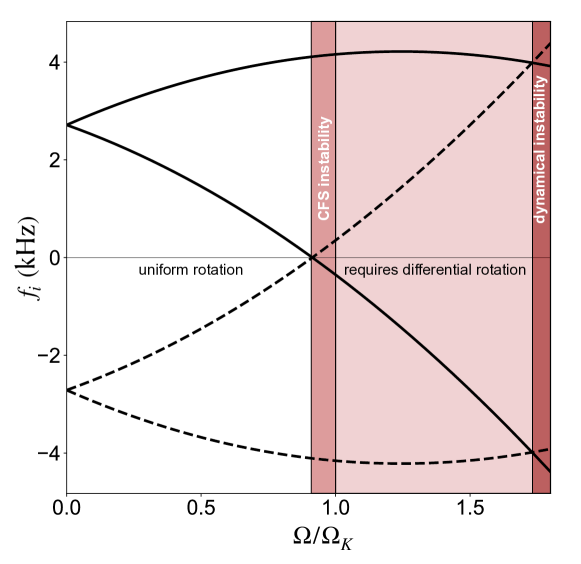
Figure 2: Illustrating the numerical results from Doneva et al. (2013) for the $l=2$ f-modes of rotating neutron stars. The inertial frame mode frequency $f_{i}=\omega_{i}/2\pi$ (in kHz) is shown as function of the (uniform) rotation frequency $\Omega$ (scaled to the Kepler frequency $\Omega_{K}$).

If we want to consider the role of viscosity or consider the evolution of an unstable mode, we need dynamical mode calculation. The most detailed work in this direction builds on time-evolutions for rotating relativistic stars (typically in the Cowling approximation Gaertig and Kokkotas (2008), where variations in the metric are ignored, although see Krüger and Kokkotas (2020)). As an illustration, let us consider the results from Doneva et al. (2013) which provide empirical relations based on results for a collection of matter equations of state. For the quadrupole f-modes we have, first of all, the frequency of the mode for non-rotating stars:

$${1\over 2\pi}\omega_{0}\ \approx 1.562+1.151\left({M_{0}\over 1.4M_{\odot}}\right)^{1/2}\left({R_{0}\over 10\ \mathrm{km}}\right)^{-3/2}\ (\mathrm{kHz})\ ,$$ (75)

where $M_{0}$ and $R_{0}$ are the mass and radius of the non-rotating model, respectively. With our conventions, the inertial frame frequency of the prograde ($l=-m=2$ in the non-rotating limit) mode is (combining the results from Doneva et al. (2013) with $\omega_{i}=\omega_{r}-m\Omega$):

$$\omega_{i}=\omega_{0}\left[1-0.235\left({\Omega\over\Omega_{K}}\right)-\frac{m\Omega}{\omega_{0}}-0.358\left({\Omega\over\Omega_{K}}\right)^{2}\right]\ .$$ (76)

In this expression, the Kepler frequency, $\Omega_{K}$, is estimated by

$${1\over 2\pi}\Omega_{K}\ \approx 1.716\left({M_{0}\over 1.4M_{\odot}}\right)^{1/2}\left({R_{0}\over 10\ \mathrm{km}}\right)^{-3/2}-0.189\ (\mathrm{kHz})\ .$$ (77)

Similarly, for the retrograde ($l=m=2$) f-mode we have

$$\omega_{i}=\omega_{0}\left[1+0.402\left({\Omega\over\Omega_{K}}\right)-\frac{m\Omega}{\omega_{0}}-0.406\left({\Omega\over\Omega_{K}}\right)^{2}\right]\ .$$ (78)

In order to understand the implications of these results, we may consider the illustration in figure 2, which shows the behaviour of the modes that limit to $\pm\omega_{0}$ in the slow-rotation limit (the rotational splitting leads to a pair of modes for each $m=\pm l$). Focussing, first of all, on the pair of modes that start out with a positive frequency, we see that the frequency of the prograde $l=-m=2$ mode increases with the rotation rate. Meanwhile, the observed inertial frame frequency of the originally retrograde mode decreases and passes through zero just above $\Omega\approx 0.9\Omega_{K}$. At this point the pattern speed of the mode changes sign, signalling the onset of the CFS instability. As expected, the star has to spin very fast for the instability to kick in. Extrapolating beyond the region of validity of the results, which is cheating but serves the purpose of illustrating another important point, we see that the CFS unstable mode that started out with negative frequency eventually catches up with the originally prograde mode. The point where these two modes merge indicate the onset of dynamical instability—the so-called bar-mode instability New et al. (2000); Shibata et al. (2000); Baiotti et al. (2007). This dynamical instability requires $E_{c}=0$ which is possible when the two modes merge. This behaviour (mode merger leading to instability) is familiar from many wave problems. Beyond this point our extrapolation absolutely does not make sense, as the pair of modes would be replaced by a single complex-valued frequency once the dynamical instability sets in.

While we have no observational evidence for mature neutron stars spinning fast enough for the f-mode instability to come into play, it may be relevant for (some fraction of) newly born systems. This depends entirely on the birth-spin expected from a supernova core collapse. This issue is not particularly well understood but it is expected Spruit and Phinney (1998) that some fraction of neutron stars will be born rapidly spinning. This may, in fact, be a requirement for the dynamo mechanism needed to wind up the star’s magnetic field to magnetar strength Thompson and Duncan (1995) (but, again, the detailed mechanism for this is not understood). The unstable f-mode may also impact on the evolution of massive post-merger remnants Doneva et al. (2015). The outcome depends on, first of all, whether the spin of the system will be sufficient for the instability to be triggered and, secondly, the saturation amplitude of the unstable mode (expected to be due to the nonlinear coupling to other modes Schenk et al. (2002); Arras et al. (2003); Pnigouras and Kokkotas (2015)). It has been suggested that this kind of signal may be detectable at the distance to the Virgo cluster Doneva et al. (2015), an idea worth further consideration.

VII Final comments

In this brief overview, we have discussed aspects of neutron star seismology and how the problem connects with the rapidly developing area of gravitational-wave astronomy. The aim was to introduce the ideas rather than provide an exhaustive discussion of every possible angle. Hence, the fundamental f-mode was allowed to take centre stage throughout, at the risk of downplaying the role of other modes—like the infamous r-mode—and perhaps giving an overly simplified picture of the oscillation problem. Given this, it makes sense to conclude with some comments on the bigger picture—what we know and what we don’t know.

First of all, we are painfully aware that the oscillation problem for realistic neutron star models is complicated. Different aspects of physics tend to be associated with (more or less) distinct families of oscillation modes—composition/entropy gradients support the g-modes, the Coriolis force leads to inertial modes, there are elastic shear modes in the crust, there are superfluid modes and so on. The range of physics can be intimidating and the progress on modelling these systems in as much detail as we can muster has been fairly slow. Nevertheless, there have been notable advances.

Before going into the details it is worth going over a couple of overarching “ground rules”. First of all, it is important to keep track of the ultimate aim of the exercise: We want to combine our theory models with observations to constrain the physics. This means that—for each conceived scenario and observation channel— we must not lose track of what may be achievable with current and foreseeable technology. From the perpective of gravitational-wave astronomy (and given that neutron star dynamics tends to be a high-frequency (kHz) phenomenon) our speculation should focus on the current ground-based instruments and what may be possible with different planned 3G detectors like the Einstein Telescope or a Cosmic Explorer. In fact, clear arguments that certain aspects of neutron star physics will come within reach in the 3G era would add to the—already strong Maggiore et al. (2020)—science case for these instruments.

Secondly, we need to develop the models in the framework of general relativity (or whatever fashionable alternative theory may take our fancy). The motivation for this is simple: A realistic matter description only makes sense in the context of a relativistic stellar model. For example, it is well known that, for a given central density, the radius of a Newtonian star differs considerably from the corresponding relativistic model. The “errors” tend to be so large that any discussion of the impact of the fine print physics becomes meaningless. This does not mean that we have not learned valuable lessons from Newtonian models. On the contrary, much of our understanding of the fluid dynamics involved draws on work in the non-relativistic regime—and will likely continue to do so for some time.

With these two points in mind, let us take stock of where we stand. When it comes to studying the oscillation properties of “realistic” neutron star models, the state of the art models in Krüger et al. (2015) combine internal composition gradients with realistic cooling (including the freezing of the star’s crust) to explore the evolution of the oscillation spectrum as a young neutron star matures. These models do not account for superfluity or, indeed, the magnetic field. The former aspect is not an insurmountable challenge, given the formalism discussed in Andersson et al. (2019) and work on the torsional oscillations of the crust (motivated by the observed quasiperiodic features in the tail of some magnetar flares Samuelsson and Andersson (2009) but the magnetic field provides a technical hurdle. This is not because we are unable to study the oscillations of magnetic stars—the results from Gabler et al. (2012); Colaiuda and Kokkotas (2012) show that such work is well under way—but the simple reality is that the internal magnetic field configuration (which we need to provide a background for our perturbation analysis) is not well understood. In fact, this is a drastic understatement. None of the models we are able to build appear to be stable in the long term Lander and Jones (2012); Bera et al. (2020) and this presents us with an obvious conceptual problem. In short, we are still some way away from modelling (even non-spinning) neutron stars in their full glory. It is important that strive to do so, because the different physics aspects are not independent and we need to understand how they are linked if we want make secure inference statements for observed signals. This is particularly the case for the dynamical tide which has so far been considered only for Newtonian models. This is an issue that need attention.

When it comes to rotating relativistic stars, our models are much less complete. We have a fairly good handle on the impact of rotation on the f-mode and some idea of the effect on the pressure p-modes and the gravity g-modes Gaertig and Kokkotas (2009). This work provides an understanding of the onset of the CFS instability associated with the f-mode (for very high spin rates) Gaertig and Kokkotas (2008); Krüger et al. (2010); Gaertig et al. (2011); Doneva et al. (2013); Krüger and Kokkotas (2020), but we do not yet have a good handle on the many different dissipation mechanism that may affect an unstable mode. There is a sharp contrast between the physics that has been brought into play in efforts to “kill” the inertial r-mode instability (see Andersson (2019)) and the level of discussion for the f-mode. Having said that, the work on the r-modes is almost exclusively in the Newtonian domain so we are lacking in that respect, as well (see Lockitch et al. (2001, 2003); Idrisy et al. (2015) for a few notable exceptions). Similar statements apply to the effort to understand the saturation of unstable modes, through the nonlinear coupling to other modes Schenk et al. (2002); Arras et al. (2003); Pnigouras and Kokkotas (2015), for which a relativistic framework has not been developed. And let us not forget the phenomenology that comes into play when we add differential rotation to the mix. In particular, suggestions that the so-called low-T/W instability Centrella et al. (2001); Watts et al. (2005) may act in merger remnants are intriguing Passamonti and Andersson (2020); Xie et al. (2020); De Pietri et al. (2020). Again, this is a mechanism that is much less well understood than it ought to be. The “wish list” for rotating stars becomes quite long…

A much briefer summary would simply state that we have a lot of work left to do.