Gradient Estimate for the Heat Kernel on Some Fractal-Like Cable Systems and Quasi-Riesz Transforms

Abstract

We give pointwise upper estimate for the gradient of the heat kernel on some fractal-like cable systems including the Vicsek and the Sierpiński cable systems. Applications to $L^{p}$-boundedness of quasi-Riesz transforms are derived.

1 Introduction

Throughout the paper, the letters $C,C_{1},C_{2},C_{A},C_{B}$ will always refer to some positive constants and may change at each occurrence. The sign $\asymp$ means that the ratio of the two sides is bounded from above and below by positive constants. The sign $\lesssim$ ($\gtrsim$) means that the LHS is bounded by positive constant times the RHS from above (below).

On a complete non-compact Riemannian manifold, a celebrated result independently discovered by Grigor’yan [25] and Saloff-Coste [39, 40] is that the following two-sided Gaussian bound of the heat kernel

$$\frac{C_{1}}{V(x,\sqrt{t})}\exp\left(-C_{2}\frac{d(x,y)^{2}}{t}\right)\leq p_{t}(x,y)\leq\frac{C_{3}}{V(x,\sqrt{t})}\exp\left(-C_{4}\frac{d(x,y)^{2}}{t}\right),$$ (1)

where $V(x,r)$ denotes the Riemannian measure of the open geodesic ball with center $x$ and radius $r$, is equivalent to the conjunction of the volume doubling condition and the scale-invariant $L^{2}$-Poincaré inequality on balls. The proofs go through a parabolic Harnack inequality for the solutions of the heat equation, which is itself equivalent to (1).

However, the matching upper estimate of the gradient of the heat kernel

$$|\nabla_{y}p_{t}(x,y)|\leq\frac{C_{1}}{\sqrt{t}V(x,\sqrt{t})}\exp\left(-C_{2}\frac{d(x,y)^{2}}{t}\right)$$

only holds in some cases, for example, Riemannian manifolds with non-negative Ricci curvature [37], Lie groups with polynomial volume growth [38] and covering manifolds with polynomial volume growth [22, 23].

Pointwise or (weighted) $L^{p}$-bounds for the gradient of the heat kernel play an important role in the $L^{p}$-boundedness of the Riesz transform for $p>2$. On a complete non-compact Riemannian manifold, it is obvious that $\lVert|\nabla u|\rVert_{2}=\lVert\Delta^{1/2}u\rVert_{2}$ for any smooth function $u$ with compact support, hence the Riesz transform $\nabla\Delta^{-1/2}$ is $L^{2}$-bounded. Strichartz [42] formulated the following question: for which values of $p\in(1,+\infty)$ is the Riesz transform $\nabla\Delta^{-1/2}$ $L^{p}$-bounded? A celebrated result was given by Coulhon and Duong [19, Theorem 1.1] that the volume doubling condition and a pointwise on-diagonal upper bound of the heat kernel imply the $L^{p}$-boundedness of the Riesz transform for any $p\in(1,2]$. Moreover, this conclusion is false when $p>2$, as the counterexample given by the connected sum of two copies of $\mathbb{R}^{n}$ shows ([19, Section 5]). For $p>2$, Auscher, Coulhon, Duong and Hofmann [5, Theorem 1.3] proved that, under the volume doubling condition and the two-sided Gaussian bound of the heat kernel, the $L^{p}$-estimate of the gradient of the heat kernel is equivalent to the $L^{p}$-boundedness of the Riesz transform in some proper sense. Recently, Coulhon, Jiang, Koskela and Sikora [20] generalized the above result to metric measure spaces endowed with a Dirichlet form deriving from a “carré du champ” and improved the results of [5], even in the case of Riemannian manifolds.

Fractals provide new examples with very different phenomena. One important estimate is the so-called sub-Gaussian bound as follows.

$$\frac{C_{1}}{V(x,t^{1/\beta})}\exp\left(-C_{2}\left(\frac{d(x,y)}{t^{1/\beta}}\right)^{\frac{\beta}{\beta-1}}\right)\leq p_{t}(x,y)\leq\frac{C_{3}}{V(x,t^{1/\beta})}\exp\left(-C_{4}\left(\frac{d(x,y)}{t^{1/\beta}}\right)^{\frac{\beta}{\beta-1}}\right),$$

where $\beta$ is a new parameter called the walk dimension which is always strictly greater than 2 on fractals. For example, on the Sierpiński gasket (see Figure 2), $\beta=\log 5/\log 2$, see [14, 34], on the Sierpiński carpet (see Figure 2), $\beta\approx 2.09697$, see [9, 10, 12, 11, 31, 36].

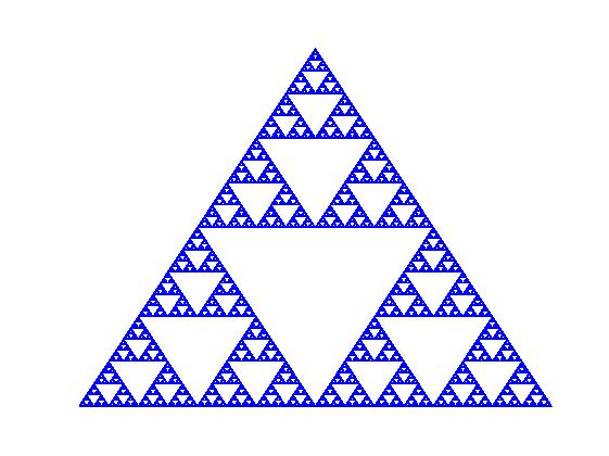
Figure 1: The Sierpiński Gasket

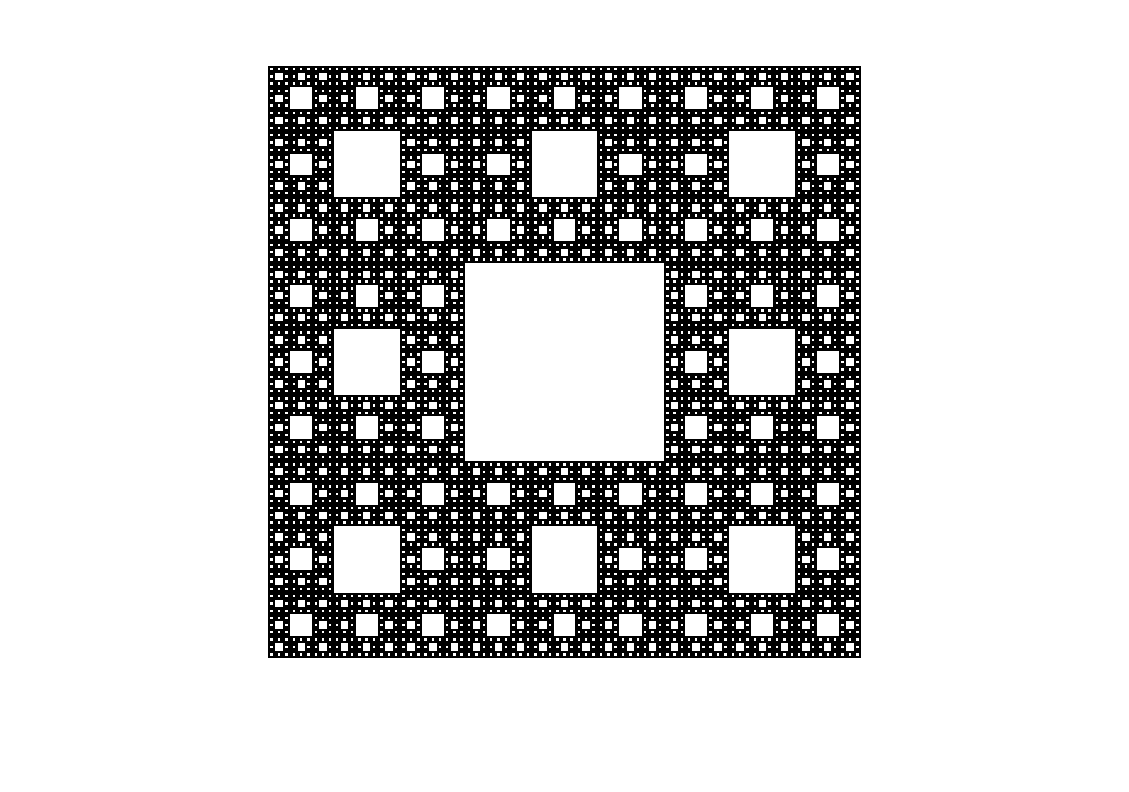
Figure 2: The Sierpiński Carpet

A natural question is to consider the matching upper estimate of the gradient of the heat kernel. However, gradient operator can not be easily defined using the classical Euclidean way due to the existence of too many “holes”. We turn to consider the corresponding fractal-like manifolds or fractal-like cable systems. Roughly speaking, given a fractal, by translating the small scale self-similar property, we obtain an infinite graph with self-similar property in the large scale. If we replace each edge of the graph by a tube and glue these tubes smoothly at each vertex, then we obtain a fractal-like manifold where the gradient operator is the standard one on a Riemannian manifold. If we replace each edge of the graph by an interval, then we obtain a fractal-like cable system where the gradient operator can be defined as the usual derivative on each interval (although only one-sided derivatives are well-defined at the endpoints of each interval, it does not matter since the set of all the endpoints has measure zero in our consideration).

On a fractal-like manifold or a fractal-like cable system, one can consider the Riesz transform. Chen, Coulhon, Feneuil and the second author [18] proved that the volume doubling condition and the sub-Gaussian heat kernel upper bound imply the $L^{p}$-boundedness of the Riesz transform for any $p\in(1,2]$. They also proved that in the Vicsek case, the Riesz transform is $L^{p}$-bounded if and only if $p\in(1,2]$, where the fact that the Vicsek set is a tree was intrinsically used to do some explicit calculations of the $L^{p}$-norms of harmonic functions. Amenta [2] generalized the $L^{p}$-unboundedness for $p>2$ to other Riemannian manifolds that satisfy the so-called spinal condition which can be regarded as a weaker form of the tree condition.

In this paper, we consider some fractal-like cable systems satisfying certain geometric and functional assumptions, and obtain pointwise upper bound for the gradient of the heat kernel as well as the $L^{p}$-boundedness for the “quasi-Riesz transforms”, which are a suitable variant of the Riesz transform.

Our first main result is a pointwise gradient upper estimate for the heat kernel on a cable system $X$ under some assumptions, which we only roughly describe here (the precise definitions of which will be given in Section 2). The assumptions on $X$ involve two positive parameters $\alpha$ and $\beta$ satisfying $2\leq\beta\leq\alpha+1$ and two functions $\Phi$ and $\Psi$ defined on $(0,+\infty)$ given by

$$\begin{split}\Phi(r)&=r1_{(0,1)}(r)+r^{\alpha}1_{[1,+\infty)}(r),\\ \Psi(r)&=r^{2}1_{(0,1)}(r)+r^{\beta}1_{[1,+\infty)}(r).\end{split}$$ (2)

Denote by $d$ (resp. $m$) the metric (resp. the measure) on $X$. Consider also a strongly local regular Dirichlet form $(\mathcal{E},\mathcal{F})$ on $L^{2}(X;m)$. Let $V(x,r)$ denote the measure of the open ball with center $x\in X$ and radius $r\in(0,+\infty)$. The assumption V($\Phi$) means that $V(x,r)\asymp\Phi(r)$.

To establish pointwise gradient estimate for the heat kernel, we need to assume a pointwise upper bound for the heat kernel itself, that is, say that UHK($\Psi$) holds if

$$p_{t}(x,y)\leq\frac{1}{V\left(x,\Psi^{-1}(C_{1}t)\right)}\exp\left(-\Upsilon\left(C_{2}d(x,y),t\right)\right),$$

where

$$\Upsilon(R,t)=\sup_{s\in(0,+\infty)}\left(\frac{R}{s}-\frac{t}{\Psi(s)}\right),$$

and a reverse Hölder inequality for the gradients of harmonic functions. Recall that such inequalities play a key role in the study of the $L^{p}$-boundedness of the Riesz transform for $p>2$, see [4, 15, 20]. The classical statement for the reverse Hölder inequality is as follows: say that the reverse Hölder inequality for the gradients of harmonic functions holds if there exists $C_{H}\in(0,+\infty)$ such that for any ball $B$ with radius $r$, for any function $u$ harmonic in $2B$, we have

$$\left\|\left|\nabla u\right|\right\|_{L^{\infty}(B)}\leq\frac{C_{H}}{r}\mathchoice{{\vbox{\hbox{$\textstyle-$ }}\kern-7.83337pt}}{{\vbox{\hbox{$\scriptstyle-$ }}\kern-5.90005pt}}{{\vbox{\hbox{$\scriptscriptstyle-$ }}\kern-4.75003pt}}{{\vbox{\hbox{$\scriptscriptstyle-$ }}\kern-4.25003pt}}\!\int_{2B}\left|u\right|\mathrm{d}m$$

(the precise definition of $\left|\nabla u\right|$ will be given at the end of Section 2). The reverse Hölder inequality holds on the $N$-dimensional Vicsek cable system for any $N\geq 2$, see Proposition 4.1. However, this condition does not hold on the Sierpiński cable system, see Proposition 4.2. This leads us to introduce a new condition, called a generalized reverse Hölder inequality for the gradients of harmonic functions, which also holds on the Vicsek cable systems, see Proposition 4.3. More precisely, say that the generalized reverse Hölder inequality GRH($\Phi,\Psi$) holds if there exists $C_{H}\in(0,+\infty)$ such that for any ball $B$ with radius $r$, for any function $u$ harmonic in $2B$, we have

$$\lVert|\nabla u|\rVert_{L^{\infty}(B)}\leq C_{H}\frac{\Phi(r)}{\Psi(r)}\mathchoice{{\vbox{\hbox{$\textstyle-$ }}\kern-7.83337pt}}{{\vbox{\hbox{$\scriptstyle-$ }}\kern-5.90005pt}}{{\vbox{\hbox{$\scriptscriptstyle-$ }}\kern-4.75003pt}}{{\vbox{\hbox{$\scriptscriptstyle-$ }}\kern-4.25003pt}}\!\int_{2B}|u|\mathrm{d}m.$$

Our first main result states as follows.

Theorem 1.1.

Let $(X,d,m,\mathcal{E},\mathcal{F})$ be an unbounded cable system satisfying V($\Phi$), UHK($\Psi$) and GRH($\Phi,\Psi$). We have the gradient estimate GHK($\Phi,\Psi$) for the heat kernel as follows: there exist $C_{1},C_{2},C_{3},C_{4}\in(0,+\infty)$ such that for any $t\in(0,+\infty)$, for $m$-a.e. $x,y\in X$, we have

$$|\nabla_{y}p_{t}(x,y)| \leq\frac{\Phi(\Psi^{-1}(t))}{tV\left(x,\Psi^{-1}(C_{1}t)\right)}\exp\left(-\Upsilon\left(C_{2}d(x,y),t\right)\right)$$

$$\leq\begin{cases}\frac{C_{3}}{\sqrt{t}V(x,\sqrt{t})}\exp\left(-C_{4}\frac{d(x,y)^{2}}{t}\right),&\text{if }t\in(0,1),\\ \frac{C_{3}}{t^{1-\frac{\alpha}{\beta}}V(x,t^{1/\beta})}\exp\left(-C_{4}\left(\frac{d(x,y)}{t^{{1}/{\beta}}}\right)^{\frac{\beta}{\beta-1}}\right),&\text{if }t\in[1,+\infty).\end{cases} \Phi,\Psi$$ GHK()

In particular, GHK($\Phi,\Psi$) holds on the $N$-dimensional Vicsek cable system with $\alpha=\log(2^{N}+1)/\log 3$, $\beta=\log(3\cdot(2^{N}+1))/\log 3$ for any $N\geq 2$ and on the Sierpiński cable system with $\alpha=\log 3/\log 2$ and $\beta=\log 5/\log 2$.

To the best of our knowledge, this is the first pointwise upper bound for the gradient of the heat kernel in a sub-Gaussian type context.

Remark 1.2.

Arguing as in the proof of Theorem 1.1, we also prove the following result. For any $p\in(1,+\infty)$, there exist $\gamma,C\in(0,+\infty)$ such that for $m$-a.e. $y\in X$, we have

$$\left\||\nabla p_{t}(\cdot,y)|\exp\left(\gamma\frac{d(\cdot,y)^{2}}{t}\right)\right\|_{p}\leq\frac{C}{\sqrt{t}\left[V(y,\sqrt{t})\right]^{1-\frac{1}{p}}}\text{ if }t\in(0,1),$$

and

$$\left\||\nabla p_{t}(\cdot,y)|\exp\left(\gamma\left(\frac{d(\cdot,y)}{t^{1/\beta}}\right)^{\frac{\beta}{\beta-1}}\right)\right\|_{p}\leq\frac{C}{t^{1-\frac{\alpha}{\beta}}\left[V(y,t^{1/\beta})\right]^{1-\frac{1}{p}}}\text{ if }t\in[1,+\infty).$$ (3)

For $p\in(1,2)$, it was proved in [18, Lemma 2.2] that, on any general Riemannian manifold or graph $M$ satisfying VD and UHK($\Psi$) (no reverse Hölder inequality is required), the following weighted $L^{p}$-estimate for the gradient of the heat kernel holds: there exist $\gamma,C\in(0,+\infty)$ such that for any $y\in M$, we have

$$\left\|\left|\nabla p_{t}(\cdot,y)\right|\exp\left(\gamma\frac{d(\cdot,y)^{2}}{t}\right)\right\|_{p}\leq\frac{C}{\sqrt{t}\left[V(y,\sqrt{t})\right]^{1-\frac{1}{p}}}\text{ if }t\in(0,1),$$

and

$$\left\|\left|\nabla p_{t}(\cdot,y)\right|\exp\left(\gamma\left(\frac{d(\cdot,y)}{t^{1/\beta}}\right)^{\frac{\beta}{\beta-1}}\right)\right\|_{p}\leq\frac{C}{\sqrt{t}\left[V(y,t^{1/{\beta}})\right]^{1-\frac{1}{p}}}\text{ if }t\in[1,+\infty).$$ (4)

Since $2\alpha\geq\alpha+1\geq\beta$, which entails $1-\frac{\alpha}{\beta}\leq\frac{1}{2}$, it follows that for $p\in(1,2)$, the conclusion of Theorem 1.1 is weaker than the one of [18, Lemma 2.2], that is, (3) is weaker than (4). On the other hand, (4) is limited to the range $p\in(1,2)$, and no pointwise estimate for the gradient of the heat kernel was proved in [18]. In fact, it is unlikely that the corresponding pointwise estimate for the gradient of the heat kernel holds under VD and UHK($\Psi$) only.

From Theorem 1.1, we easily obtain another bound for $\left|\nabla p_{t}\right|$, assuming a two-sided bound for $p_{t}$. Namely, say that the heat kernel bound HK($\Psi$) holds if

$$\frac{1}{V\left(x,\Psi^{-1}(C_{1}t)\right)}\exp\left(-\Upsilon\left(C_{2}d(x,y),t\right)\right)\leq p_{t}(x,y)\leq\frac{1}{V\left(x,\Psi^{-1}(C_{3}t)\right)}\exp\left(-\Upsilon\left(C_{4}d(x,y),t\right)\right).$$

Then, it is plain to deduce from Theorem 1.1 the following result:

Corollary 1.3.

Let $(X,d,m,\mathcal{E},\mathcal{F})$ be an unbounded cable system satisfying V($\Phi$), HK($\Psi$) and GRH($\Phi,\Psi$). Then there exist $C_{1},C_{2}\in(0,+\infty)$ such that for any $t\in(0,+\infty)$, for $m$-a.e. $x,y\in X$, we have

$$\left|\nabla_{y}p_{t}(x,y)\right|\leq C_{1}\frac{\Phi(\Psi^{-1}(t))}{t}p_{C_{2}t}(x,y).$$

Note that this is similar to the classical estimate for $\left|\nabla p_{t}\right|$ on Riemannian manifolds with non-negative Ricci curvature (with $C_{1}=C_{2}=1$ in this case), see [37].

The strategy of our proof is to use the fact that the heat kernel is a solution of the heat equation which can be regarded as a Poisson equation for a fixed time. Since the regularity of the time derivative of the heat kernel is easy to handle, one only needs to have gradient estimates for the solutions of Poisson equation; this has been the approach considered in [33, 20]. In their settings, the local quantitative Lipschitz regularity for Cheeger-harmonic functions [33, Theorem 3.1] or the reverse Hölder inequality for the gradients of harmonic functions [20, Theorem 3.2] which are consequences of some curvature assumptions was needed. In the present work, we rely on the approach through the generalized reverse Hölder inequality, see Proposition 5.1.

Our second main result is the $L^{p}$-boundedness of the “quasi-Riesz transforms” for any $p\in(1,+\infty)$ in the fractal setting. Recall that, under the volume doubling condition and the sub-Gaussian pointwise upper bound for the heat kernel, it was proved in [18, Theorem 1.2] that the Riesz transform $\nabla\Delta^{-1/2}$ is $L^{p}$-bounded for any $p\in(1,2]$. In [5], the $L^{p}$-boundedness of the Riesz transform for some values of $p>2$ was derived from an $L^{p}$-bound for the gradient of the heat semi-group, where the volume doubling condition and the scale-invariant $L^{2}$-Poincaré inequality are assumed to hold (recall that, in this situation, pointwise Gaussian upper and lower bounds for the heat kernel hold). This contrasts with the sub-Gaussian context. Indeed, in the case of the Vicsek cable systems, the Riesz transform is $L^{p}$-unbounded for any $p>2$, see [18, Theorem 5.1], while a pointwise sub-Gaussian bound for the gradient of the heat kernel holds, as Theorem 1.1 shows (note that an $L^{2}$-Poincaré inequality on balls, with a nonstandard scaling, still holds in this case).

Motivated by situations where the heat kernel satisfies sub-Gaussian upper bound, consider a weaker form of the Riesz transform, namely the quasi-Riesz transform, where the exponent ${1}/{2}$ is replaced by some $\varepsilon\in(0,{1}/{2})$. The quasi-Riesz transforms were introduced in [17], as a substitute of the Riesz transform. We also rely on the decomposition of the Riesz transform as the sum of a local part and a global one (this idea goes back to [1]), which was also pushed further in [17]. More precisely, if $p\in(1,+\infty)$, say that the local Riesz transform is $L^{p}$-bounded if and only if

$$\lVert|\nabla f|\rVert_{p}\lesssim\lVert(I+\Delta)^{{1}/{2}}f\rVert_{p}$$

and that the Riesz transform at infinity is $L^{p}$-bounded if and only if

$$\lVert|\nabla e^{-\Delta}f|\rVert_{p}\lesssim\lVert\Delta^{{1}/{2}}f\rVert_{p}.$$

Then the Riesz transform $\nabla\Delta^{-1/2}$ is $L^{p}$-bounded if and only if the local Riesz transform and the Riesz transform at infinity are both $L^{p}$-bounded, see [17, Theorem 2.3]. Moreover, the quasi-Riesz transform at infinity, namely $\nabla e^{-\Delta}\Delta^{-\varepsilon}$, with $\varepsilon\in(0,1/2)$, was proved in [17, Theorem 1.2] to be $L^{p}$-bounded for any $p\in(1,2]$ on any complete Riemannian manifold, without any further assumption.

Inspired by the aforementioned equivalence for the $L^{p}$-boundedness of the Riesz transform and following the approach of [5, Section 3], we establish the $L^{p}$-boundedness of the quasi-Riesz transforms for any $p\in(1,+\infty)$, as a consequence of the above gradient estimate for the heat kernel.

Theorem 1.4.

Let $(X,d,m,\mathcal{E},\mathcal{F})$ be an unbounded cable system satisfying the same assumptions as in Theorem 1.1. Then for any $\varepsilon\in(0,1-\frac{\alpha}{\beta})$, the quasi-Riesz transform $\nabla(I+\Delta)^{-1/2}+\nabla e^{-\Delta}\Delta^{-\varepsilon}$ is $L^{p}$-bounded for any $p\in(1,+\infty)$.

An interesting open question is to know whether the conclusion of Theorem 1.4 also holds for $\varepsilon=1-\frac{\alpha}{\beta}$. The exponent $\frac{\alpha}{\beta}$ in the gradient estimate for $t>1$ given by Theorem 1.1 suggests that this is the case, but the result seems more difficult to prove.

We will see from the proof of Proposition 4.3 that these results extend to the cable systems corresponding to the p.c.f. self-similar sets considered in [44] without any technical difficulty. However, it seems that more advanced techniques would be required to do the generalization to the cable system corresponding to the Sierpiński carpet which is a non-p.c.f. self-similar set and an infinitely ramified fractal.

This paper is organized as follows. In Section 2, we give some results about Poisson equation on metric measure Dirichlet spaces. In Section 3, we give formal constructions of cable systems including the Vicsek and the Sierpiński ones. In Section 4, we show that the reverse Hölder inequality holds on the Vicsek cable systems but does not hold on the Sierpiński cable system, and we show that a generalized reverse Hölder inequality holds on the Vicsek and the Sierpiński cable systems. In Section 5, we use the generalized reverse Hölder inequality to obtain gradient estimates for the solutions of Poisson equation using which we obtain gradient estimate for the heat kernel that is Theorem 1.1. In Section 6, we prove Theorem 1.4.

Acknowledgements: This work was partly supported by the French ANR project RAGE ANR-18-CE40-0012. The third author was supported by national funds through the FCT – Fundação para a Ciência e a Tecnologia, I.P. (Portuguese Foundation for Science and Technology) within the scope of the project UIDB/00297/2020 (Centro de Matemática e Aplicações).

2 Poisson Equation on Metric Measure Dirichlet Spaces

Let $(X,d,m,\mathcal{E},\mathcal{F})$ be an unbounded metric measure Dirichlet (MMD) space, that is, $(X,d)$ is a locally compact separable unbounded metric space, $m$ is a positive Radon measure on $X$ with full support, $(\mathcal{E},\mathcal{F})$ is a strongly local regular Dirichlet form on $L^{2}(X;m)$. Throughout this paper, we always assume that all metric balls are precompact.

For any $x\in X$, for any $r\in(0,+\infty)$, denote the (metric) ball $B(x,r)=\{y\in X:d(x,y)<r\}$, denote $V(x,r)=m(B(x,r))$. If $B=B(x,r)$, then we denote $\delta B=B(x,\delta r)$ for any $\delta\in(0,+\infty)$. Let $C(X)$ denote the space of all real-valued continuous functions on $X$ and let $C_{c}(X)$ denote the space of all real-valued continuous functions on $X$ with compact support.

Consider the strongly local regular Dirichlet form $(\mathcal{E},\mathcal{F})$ on $L^{2}(X;m)$. Let $\Delta$ be the corresponding generator which is a non-negative definite self-adjoint operator. Let $\Gamma$ be the corresponding energy measure. Denote $\mathcal{E}_{1}(\cdot,\cdot)=\mathcal{E}(\cdot,\cdot)+(\cdot,\cdot)$, where $(\cdot,\cdot)$ is the inner product in $L^{2}(X;m)$. We refer to [24] for related results about Dirichlet forms.

Let us now present some geometric and functional conditions on $(X,d,m,\mathcal{E},\mathcal{F})$ which will be used in the sequel. Most of them will be expressed in terms of the two functions $\Phi$ and $\Psi$ given by Equation (2).

We say that the volume doubling condition VD holds if there exists $C_{D}\in(0,+\infty)$ such that

$$V(x,2r)\leq C_{D}V(x,r)\text{ for any }x\in X,\text{ for any }r\in(0,+\infty).$$ VD

We say that the regular volume condition V($\Phi$) holds if there exists $C_{R}\in(0,+\infty)$ such that

$$\frac{1}{C_{R}}\Phi(r)\leq V(x,r)\leq C_{R}\Phi(r)\text{ for any }x\in X,\text{ for any }r\in(0,+\infty). \Phi$$ V()

It is obvious that V($\Phi$) implies VD.

2.1 Faber-Krahn, Sobolev and Poincaré Inequalities

Let $D$ be an open subset of $X$. Denote by $\lambda_{1}(D)$ the smallest Dirichlet eigenvalue for $D$, that is,

$$\lambda_{1}(D)=\inf\left\{\frac{\mathcal{E}(u,u)}{\lVert u\rVert_{2}^{2}}:u\in\mathcal{F}_{D}\backslash\left\{0\right\}\right\},$$

where

$$\mathcal{F}_{D} =\text{ the }\mathcal{E}_{1}\text{-closure of }\mathcal{F}\cap C_{c}(D).$$

We say that the relative Faber-Krahn inequality FK($\Psi$) holds if there exist $C_{F}\in(0,+\infty)$ and $\nu\in(0,1)$ such that for any ball $B=B(x,r)$, for any open subset $D$ of $B$, we have

$$\lambda_{1}(D)\geq\frac{C_{F}}{\Psi(r)}\left(\frac{m(B)}{m(D)}\right)^{\nu}. \Psi$$ FK()

We say that the local Sobolev inequality LS($\Psi$) holds if there exist $C_{L}\in(0,+\infty)$ and $q\in(2,+\infty)$ such that for any ball $B=B(x,r)$, for any $u\in\mathcal{F}_{B}$, we have

$$\left(\mathchoice{{\vbox{\hbox{$\textstyle-$ }}\kern-7.83337pt}}{{\vbox{\hbox{$\scriptstyle-$ }}\kern-5.90005pt}}{{\vbox{\hbox{$\scriptscriptstyle-$ }}\kern-4.75003pt}}{{\vbox{\hbox{$\scriptscriptstyle-$ }}\kern-4.25003pt}}\!\int_{B}|u|^{q}\mathrm{d}m\right)^{1/q}\leq C_{L}\sqrt{\Psi(r)}\left(\frac{1}{m(B)}\mathcal{E}(u,u)\right)^{1/2}, \Psi$$ LS()

where $\mathchoice{{\vbox{\hbox{$\textstyle-$ }}\kern-7.83337pt}}{{\vbox{\hbox{$\scriptstyle-$ }}\kern-5.90005pt}}{{\vbox{\hbox{$\scriptscriptstyle-$ }}\kern-4.75003pt}}{{\vbox{\hbox{$\scriptscriptstyle-$ }}\kern-4.25003pt}}\!\int_{B}=\frac{1}{m(B)}\int_{B}$.

Remark 2.1.

We will sometimes use the notations FK($\Psi,\nu$) and LS($\Psi,q$) to emphasize the role of the values of $\nu$ and $q$, respectively.

Actually, FK($\Psi$) and LS($\Psi$) are equivalent. More precisely:

Lemma 2.2.

Let $(X,d,m,\mathcal{E},\mathcal{F})$ be an unbounded MMD space. Then FK($\Psi$) is equivalent to LS($\Psi$) with $q=\frac{2}{1-\nu}$ or $\nu=1-\frac{2}{q}$.

The fact that Faber-Krahn and Sobolev inequalities are equivalent in quite general contexts was already proved several times (see [16, 6], for instance). Since the Faber-Krahn and the local Sobolev inequalities under consideration in the present paper involve the function $\Psi$, we provide a proof here for the sake of completeness.

Proof.

The proof is inspired by [27, Exercise 14.6]. “$\Leftarrow$”: Let $D$ be an open subset of a ball $B=B(x,r)$. For any $u\in\mathcal{F}_{D}\backslash\left\{0\right\}$, by LS($\Psi,q$), we have

$$\lVert u\rVert_{2}^{2} =\int_{D}|u|^{2}\mathrm{d}m\leq\left(\int_{D}|u|^{2\cdot\frac{q}{2}}\mathrm{d}m\right)^{\frac{2}{q}}\left(\int_{D}1\mathrm{d}m\right)^{1-\frac{2}{q}}=\left(\int_{B}|u|^{q}\mathrm{d}m\right)^{\frac{2}{q}}m(D)^{1-\frac{2}{q}}$$

$$\leq C_{L}^{2}\Psi(r)m(B)^{\frac{2}{q}-1}\mathcal{E}(u,u)m(D)^{1-\frac{2}{q}}=C_{L}^{2}\Psi(r)\left(\frac{m(D)}{m(B)}\right)^{1-\frac{2}{q}}\mathcal{E}(u,u),$$

hence

$$\frac{\mathcal{E}(u,u)}{\lVert u\rVert_{2}^{2}}\geq\frac{1}{C_{L}^{2}\Psi(r)}\left(\frac{m(B)}{m(D)}\right)^{1-\frac{2}{q}}.$$

Taking the infimum with respect to $u\in\mathcal{F}_{D}\backslash\left\{0\right\}$, we have

$$\lambda_{1}(D)\geq\frac{1}{C_{L}^{2}\Psi(r)}\left(\frac{m(B)}{m(D)}\right)^{1-\frac{2}{q}},$$

that is, we have FK($\Psi,\nu$) with $\nu=1-\frac{2}{q}$ and $C_{F}=\frac{1}{C_{L}^{2}}$.

“$\Rightarrow$”: Firstly, let $u\in\mathcal{F}\cap C_{c}(B)$ be non-negative. Take $p\in(1,+\infty)$. For any $k\in\mathbb{Z}$, let $\Omega_{k}=\left\{u>2^{k}\right\}$ and $m_{k}=m(\overline{\Omega_{k}})$, then

$$\int_{B}u^{2p}\mathrm{d}m=\sum_{k\in\mathbb{Z}}\int_{\Omega_{k}\backslash\Omega_{k+1}}u^{2p}\mathrm{d}m\leq 4^{p}\sum_{k\in\mathbb{Z}}4^{pk}m_{k}.$$

For any $k\in\mathbb{Z}$, let $u_{k}=\left(u-2^{k}\right)^{+}\wedge 2^{k}$, then $u_{k}\in\mathcal{F}\cap C_{c}(B)$ satisfies

$$\Gamma(u_{k},u_{k})|_{\Omega_{k}\backslash\Omega_{k+1}}=\Gamma(u,u)|_{\Omega_{k}\backslash\Omega_{k+1}},\Gamma(u_{k},u_{k})|_{X\backslash(\Omega_{k}\backslash\Omega_{k+1})}=0,$$

then

$$\mathcal{E}(u,u) =\sum_{k\in\mathbb{Z}}\int_{\Omega_{k}\backslash\Omega_{k+1}}\mathrm{d}\Gamma(u,u)=\sum_{k\in\mathbb{Z}}\int_{\Omega_{k}\backslash\Omega_{k+1}}\mathrm{d}\Gamma(u_{k},u_{k})$$

$$=\sum_{k\in\mathbb{Z}}\int_{X}\mathrm{d}\Gamma(u_{k},u_{k})=\sum_{k\in\mathbb{Z}}\mathcal{E}(u_{k},u_{k}).$$

For any $k\in\mathbb{Z}$, using the facts that $u\in C_{c}(B)$ and that $m$ is regular, choose an open set $\widetilde{\Omega}_{k}$ satisfying $\overline{\Omega_{k}}\subseteq\widetilde{\Omega}_{k}\subseteq B$ and $m(\widetilde{\Omega}_{k})\leq 2m(\overline{\Omega_{k}})=2m_{k}$, then $u_{k}\in\mathcal{F}_{\widetilde{\Omega}_{k}}$. By FK($\Psi,\nu$), we have

$$\lambda_{1}(\widetilde{\Omega}_{k})\geq\frac{C_{F}}{\Psi(r)}\left(\frac{m(B)}{m(\widetilde{\Omega}_{k})}\right)^{\nu}\geq\frac{C_{F}}{\Psi(r)}\left(\frac{m(B)}{2m_{k}}\right)^{\nu},$$

hence

$$\mathcal{E}(u_{k},u_{k})\geq\frac{C_{F}}{\Psi(r)}\left(\frac{m(B)}{2m_{k}}\right)^{\nu}\lVert u_{k}\rVert^{2}_{2},$$

hence

$$\mathcal{E}(u,u)=\sum_{k\in\mathbb{Z}}\mathcal{E}(u_{k},u_{k})\geq\sum_{k\in\mathbb{Z}}\frac{C_{F}}{\Psi(r)}\left(\frac{m(B)}{2m_{k}}\right)^{\nu}\lVert u_{k}\rVert_{2}^{2},$$

where

$$\lVert u_{k}\rVert_{2}^{2}=\int_{X}u_{k}^{2}\mathrm{d}m\geq\int_{\overline{\Omega_{k+1}}}u_{k}^{2}\mathrm{d}m\geq 4^{k}m_{k+1},$$

hence

$$\mathcal{E}(u,u)\geq\frac{C_{F}m(B)^{\nu}}{2^{\nu}\Psi(r)}\sum_{k\in\mathbb{Z}}\frac{4^{k}m_{k+1}}{m_{k}^{\nu}}.$$

Let $r,s>1$ satisfy $1/r+1/s=1$. For any positive sequences $\left\{x_{k}\right\}$, $\left\{y_{k}\right\}$, we have

$$\sum x_{k}\leq\left(\sum x_{k}^{1/r}\right)^{r}\leq\left(\sum\frac{x_{k}}{y_{k}}\right)\left(\sum y_{k}^{\frac{s}{r}}\right)^{\frac{r}{s}}.$$

Hence for any $\alpha\in(0,+\infty)$, we have

$$\sum x_{k}\leq\left(\sum\frac{x_{k}}{y_{k}}\right)\left(\sum y_{k}^{\alpha}\right)^{\frac{1}{\alpha}}.$$

Therefore,

$$\sum_{k\in\mathbb{Z}}4^{pk}m_{k}=4^{p}\sum_{k\in\mathbb{Z}}4^{pk}m_{k+1}$$

$$\leq 4^{p}\left(\sum_{k\in\mathbb{Z}}\frac{4^{pk}m_{k+1}}{4^{(p-1)k}m_{k}^{\nu}}\right)\left(\sum_{k\in\mathbb{Z}}\left(4^{(p-1)k}m_{k}^{\nu}\right)^{\alpha}\right)^{\frac{1}{\alpha}}$$

$$=4^{p}\left(\sum_{k\in\mathbb{Z}}\frac{4^{k}m_{k+1}}{m_{k}^{\nu}}\right)\left(\sum_{k\in\mathbb{Z}}4^{\alpha(p-1)k}m_{k}^{\alpha\nu}\right)^{\frac{1}{\alpha}}.$$

Take $\alpha=\frac{1}{\nu}$ and $p:=\frac{1}{1-\nu}$, so that $\alpha(p-1)=p$. Then

$$\sum_{k\in\mathbb{Z}}4^{pk}m_{k}\leq 4^{p}\left(\sum_{k\in\mathbb{Z}}\frac{4^{k}m_{k+1}}{m_{k}^{\nu}}\right)\left(\sum_{k\in\mathbb{Z}}4^{pk}m_{k}\right)^{1-\frac{1}{p}},$$

hence

$$\left(\sum_{k\in\mathbb{Z}}4^{pk}m_{k}\right)^{\frac{1}{p}}\leq 4^{p}\sum_{k\in\mathbb{Z}}\frac{4^{k}m_{k+1}}{m_{k}^{\nu}},$$

so

$$\int_{B}u^{2p}\mathrm{d}m\leq 4^{p}\sum_{k\in\mathbb{Z}}4^{pk}m_{k}\leq 4^{p}\left(4^{p}\sum_{k\in\mathbb{Z}}\frac{4^{k}m_{k+1}}{m_{k}^{\nu}}\right)^{p}\leq 4^{p}\left(4^{p}\frac{2^{\nu}\Psi(r)}{C_{F}m(B)^{\nu}}\mathcal{E}(u,u)\right)^{p},$$

that is,

$$\left(\mathchoice{{\vbox{\hbox{$\textstyle-$ }}\kern-7.83337pt}}{{\vbox{\hbox{$\scriptstyle-$ }}\kern-5.90005pt}}{{\vbox{\hbox{$\scriptscriptstyle-$ }}\kern-4.75003pt}}{{\vbox{\hbox{$\scriptscriptstyle-$ }}\kern-4.25003pt}}\!\int_{B}u^{2p}\mathrm{d}m\right)^{\frac{1}{2p}}\leq\frac{2^{p+\frac{3}{2}-\frac{1}{2p}}}{\sqrt{C_{F}}}\sqrt{\Psi(r)}\left(\frac{1}{m(B)}\mathcal{E}(u,u)\right)^{1/2}.$$

Letting $q=2p=\frac{2}{1-\nu}$, we have the desired result with $C_{L}=\frac{2^{\frac{q}{2}+\frac{3}{2}-\frac{1}{q}}}{\sqrt{C_{F}}}$.

Secondly, let $u\in\mathcal{F}\cap C_{c}(B)$. Then $|u|\in\mathcal{F}\cap C_{c}(B)$ is non-negative. By the first case, we have

$$\left(\mathchoice{{\vbox{\hbox{$\textstyle-$ }}\kern-7.83337pt}}{{\vbox{\hbox{$\scriptstyle-$ }}\kern-5.90005pt}}{{\vbox{\hbox{$\scriptscriptstyle-$ }}\kern-4.75003pt}}{{\vbox{\hbox{$\scriptscriptstyle-$ }}\kern-4.25003pt}}\!\int_{B}|u|^{q}\mathrm{d}m\right)^{1/q} \leq C_{L}\sqrt{\Psi(r)}\left(\frac{1}{m(B)}\mathcal{E}(|u|,|u|)\right)^{1/2}$$

$$\leq C_{L}\sqrt{\Psi(r)}\left(\frac{1}{m(B)}\mathcal{E}(u,u)\right)^{1/2}.$$

Thirdly, let $u\in\mathcal{F}_{B}$. Then there exists $\left\{u_{k}\right\}\subseteq\mathcal{F}\cap C_{c}(B)$ which is $\mathcal{E}_{1}$-convergent to $u$, therefore there exists a subsequence still denoted by $\left\{u_{k}\right\}$ that converges to $u$ $m$-a.e., hence

$$\left(\mathchoice{{\vbox{\hbox{$\textstyle-$ }}\kern-7.83337pt}}{{\vbox{\hbox{$\scriptstyle-$ }}\kern-5.90005pt}}{{\vbox{\hbox{$\scriptscriptstyle-$ }}\kern-4.75003pt}}{{\vbox{\hbox{$\scriptscriptstyle-$ }}\kern-4.25003pt}}\!\int_{B}|u|^{q}\mathrm{d}m\right)^{1/q}\leq\varliminf_{k\to+\infty}\left(\mathchoice{{\vbox{\hbox{$\textstyle-$ }}\kern-7.83337pt}}{{\vbox{\hbox{$\scriptstyle-$ }}\kern-5.90005pt}}{{\vbox{\hbox{$\scriptscriptstyle-$ }}\kern-4.75003pt}}{{\vbox{\hbox{$\scriptscriptstyle-$ }}\kern-4.25003pt}}\!\int_{B}|u_{k}|^{q}\mathrm{d}m\right)^{1/q}$$

$$\leq\varliminf_{k\to+\infty}C_{L}\sqrt{\Psi(r)}\left(\frac{1}{m(B)}\mathcal{E}(u_{k},u_{k})\right)^{1/2}$$

$$=C_{L}\sqrt{\Psi(r)}\left(\frac{1}{m(B)}\mathcal{E}(u,u)\right)^{1/2}.$$

∎

Let $U$, $V$ be two open subsets of $X$ satisfying $U\subseteq\overline{U}\subseteq V$. We say that $\varphi\in\mathcal{F}$ is a cutoff function for $U\subseteq V$ if $0\leq\varphi\leq 1$ $m$-a.e., $\varphi=1$ $m$-a.e. in an open neighborhood of $\overline{U}$ and $\mathrm{supp}(\varphi)\subseteq V$, where $\mathrm{supp}(f)$ refers to the support of the measure $|f|\mathrm{d}m$ for any given function $f$.

We say that the cutoff Sobolev inequality CS($\Psi$) holds if there exists $C_{S}\in(0,+\infty)$ such that for any $x\in X$, for any $R,r\in(0,+\infty)$, there exists a cutoff function $\varphi\in\mathcal{F}$ for $B(x,R)\subseteq B(x,R+r)$ such that for any $f\in\mathcal{F}$, we have

$$\int_{B(x,R+r)\backslash\overline{B(x,R)}}f^{2}\mathrm{d}\Gamma(\varphi,\varphi)$$

$$\leq\frac{1}{8}\int_{B(x,R+r)\backslash\overline{B(x,R)}}\varphi^{2}\mathrm{d}\Gamma(f,f)+\frac{C_{S}}{\Psi(r)}\int_{B(x,R+r)\backslash\overline{B(x,R)}}f^{2}\mathrm{d}m. \Psi$$ CS()

We say that the Poincaré inequality PI($\Psi$) holds if there exists $C_{P}\in(0,+\infty)$ such that for any ball $B=B(x,r)$, for any $u\in\mathcal{F}$, we have

$$\int_{B}|u-u_{B}|^{2}\mathrm{d}m\leq C_{P}\Psi(r)\int_{2B}\mathrm{d}\Gamma(u,u), \Psi$$ PI()

where $u_{A}$ is the mean value of $u$ on a measurable set $A$ with $m(A)\in(0,+\infty)$, that is,

$$u_{A}=\mathchoice{{\vbox{\hbox{$\textstyle-$ }}\kern-7.83337pt}}{{\vbox{\hbox{$\scriptstyle-$ }}\kern-5.90005pt}}{{\vbox{\hbox{$\scriptscriptstyle-$ }}\kern-4.75003pt}}{{\vbox{\hbox{$\scriptscriptstyle-$ }}\kern-4.25003pt}}\!\int_{A}u\mathrm{d}m=\frac{1}{m(A)}\int_{A}u\mathrm{d}m.$$

2.2 Heat Kernel Estimates

Consider the regular Dirichlet form $(\mathcal{E},\mathcal{F})$ on $L^{2}(X;m)$. Let $\left\{P_{t}\right\}$ be the corresponding heat semi-group. Let $\left\{X_{t},t\geq 0,\mathbb{P}_{x},x\in X\backslash\mathcal{N}_{0}\right\}$ be the corresponding Hunt process, where $\mathcal{N}_{0}$ is a properly exceptional set, that is, $m(\mathcal{N}_{0})=0$ and $\mathbb{P}_{x}(X_{t}\in\mathcal{N}_{0}\text{ for some }t>0)=0$ for any $x\in X\backslash\mathcal{N}_{0}$. For any bounded Borel function $f$, we have $P_{t}f(x)=\mathbb{E}_{x}f(X_{t})$ for any $t>0$, for any $x\in X\backslash\mathcal{N}_{0}$.

The heat kernel $p_{t}(x,y)$ associated with the heat semi-group $\left\{P_{t}\right\}$ is a measurable function defined on $(0,+\infty)\times(X\backslash\mathcal{N}_{0})\times(X\backslash\mathcal{N}_{0})$ satisfying that:

• For any bounded Borel function $f$, for any $t>0$, for any $x\in X\backslash\mathcal{N}_{0}$, we have

  $$P_{t}f(x)=\int_{X\backslash\mathcal{N}_{0}}p_{t}(x,y)f(y)m(\mathrm{d}y).$$

• For any $t,s>0$, for any $x,y\in X\backslash\mathcal{N}_{0}$, we have

  $$p_{t+s}(x,y)=\int_{X\backslash\mathcal{N}_{0}}p_{t}(x,z)p_{s}(z,y)m(\mathrm{d}z).$$

• For any $t>0$, for any $x,y\in X\backslash\mathcal{N}_{0}$, we have $p_{t}(x,y)=p_{t}(y,x)$.

See [30] for more details.

We say that the heat kernel upper bound UHK($\Psi$) holds if there exist a properly exceptional set $\mathcal{N}$ and $C_{1}$, $C_{2}\in(0,+\infty)$ such that for any $t\in(0,+\infty)$, for any $x,y\in X\backslash\mathcal{N}$, we have

$$p_{t}(x,y)\leq\frac{1}{V\left(x,\Psi^{-1}(C_{1}t)\right)}\exp\left(-\Upsilon\left(C_{2}d(x,y),t\right)\right), \Psi$$ UHK()

where

$$\Upsilon(R,t)=\sup_{s\in(0,+\infty)}\left(\frac{R}{s}-\frac{t}{\Psi(s)}\right)\asymp\begin{cases}\frac{R^{2}}{t},&\text{if }t<R,\\ \left(\frac{R}{t^{1/\beta}}\right)^{\frac{\beta}{\beta-1}},&\text{if }t\geq R.\end{cases}$$

Then UHK($\Psi$) can also be re-written as follows:

$$p_{t}(x,y)\leq\begin{cases}\frac{1}{V\left(x,\Psi^{-1}(C_{1}t)\right)}\exp\left(-C_{2}\frac{d(x,y)^{2}}{t}\right),&\text{if }t<d(x,y),\\ \frac{1}{V\left(x,\Psi^{-1}(C_{1}t)\right)}\exp\left(-C_{2}\left(\frac{d(x,y)}{t^{1/\beta}}\right)^{\frac{\beta}{\beta-1}}\right),&\text{if }t\geq d(x,y).\end{cases}$$

If a lower bound, similar to UHK($\Psi$), with different constants $C_{i}$ also holds, then we say that HK($\Psi$) holds. Note that, in [29], a lower bound for $p_{t}$, called the near-diagonal lower bound $(NLE)_{\Psi}$, is written as

$$p_{t}(x,y)\geq\frac{c}{V(x,\Psi^{-1}(t))} (NLE)_{\Psi}$$

for any $t>0$ and $m$-a.e. $x,y\in X$ such that $d(x,y)\leq\varepsilon\Psi^{-1}(t)$ where $c,\varepsilon>0$ are constants independent of $t,x,y$. But [13, THEOREM 3.2] ensures that, if the metric $d$ is furthermore assumed to be geodesic, which is the case of cable systems, then the conjunction of UHK($\Psi$) and $(NLE)_{\Psi}$ is equivalent to HK($\Psi$).

Observe that the function $\beta\mapsto\left(\frac{d(x,y)}{t^{1/\beta}}\right)^{\frac{\beta}{\beta-1}}$ is monotone decreasing if $d(x,y)>t$ and monotone increasing if $d(x,y)\leq t$. Indeed,

$$\log\left(\frac{d(x,y)}{t^{1/\beta}}\right)^{\frac{\beta}{\beta-1}}=\log d(x,y)+\frac{1}{\beta-1}\log\frac{d(x,y)}{t}.$$

Assume now that $d(x,y)\leq t$, so that

$$p_{t}(x,y)\leq\frac{1}{V\left(x,\Psi^{-1}(C_{1}t)\right)}\exp\left(-C_{2}\left(\frac{d(x,y)}{t^{1/\beta}}\right)^{\frac{\beta}{\beta-1}}\right).$$

Since $\beta\geq 2$, the aforementioned monotonicity therefore yields

$$\frac{d(x,y)^{2}}{t}\leq\left(\frac{d(x,y)}{t^{1/\beta}}\right)^{\frac{\beta}{\beta-1}},$$

which implies

$$p_{t}(x,y)\leq\frac{1}{V\left(x,\Psi^{-1}(C_{1}t)\right)}\exp\left(-C_{2}\frac{d(x,y)^{2}}{t}\right).$$

Assume now that $t<d(x,y)$. Then, arguing similarly,

$$\left(\frac{d(x,y)}{t^{1/\beta}}\right)^{\frac{\beta}{\beta-1}}\leq\frac{d(x,y)^{2}}{t},$$

therefore

$$p_{t}(x,y)\leq\frac{1}{V\left(x,\Psi^{-1}(C_{1}t)\right)}\exp\left(-C_{2}\left(\frac{d(x,y)}{t^{1/\beta}}\right)^{\frac{\beta}{\beta-1}}\right).$$

Thus, UHK($\Psi$) implies that

$$p_{t}(x,y) \leq\begin{cases}\frac{1}{V\left(x,\Psi^{-1}(C_{1}t)\right)}\exp\left(-C_{2}\frac{d(x,y)^{2}}{t}\right),&\text{if }t\in(0,1),\\ \frac{1}{V\left(x,\Psi^{-1}(C_{1}t)\right)}\exp\left(-C_{2}\left(\frac{d(x,y)}{t^{1/\beta}}\right)^{\frac{\beta}{\beta-1}}\right),&\text{if }t\in[1,+\infty),\end{cases}$$

$$\asymp\begin{cases}\frac{C_{1}}{V\left(x,\sqrt{t}\right)}\exp\left(-C_{2}\frac{d(x,y)^{2}}{t}\right),&\text{if }t\in(0,1),\\ \frac{C_{1}}{V\left(x,t^{1/\beta}\right)}\exp\left(-C_{2}\left(\frac{d(x,y)}{t^{1/\beta}}\right)^{\frac{\beta}{\beta-1}}\right),&\text{if }t\in[1,+\infty).\end{cases}$$ (5)

One can characterize UHK($\Psi$) and HK($\Psi$) in terms of functional inequalities as follows:

Proposition 2.3.

([3, Theorem 1.12]) Let $(X,d,m,\mathcal{E},\mathcal{F})$ be an unbounded MMD space satisfying VD. Then the followings are equivalent.

1. FK($\Psi$) and CS($\Psi$).

2. UHK($\Psi$).

Proposition 2.4.

([29, THEOREM 1.2]) Let $(X,d,m,\mathcal{E},\mathcal{F})$ be an unbounded geodesic MMD space satisfying V($\Phi$). Then the followings are equivalent.

1. PI($\Psi$) and CS($\Psi$).

2. HK($\Psi$).

Remark 2.5.

On any complete non-compact Riemannian manifold, CS($\Psi$) with $\beta=2$ (that is, $\Psi(r)=r^{2}$ for any $r\in(0,+\infty)$) holds automatically, so that the above equivalences hold without CS($\Psi$) and are classical, see [25, 39, 26]. However, on a general MMD space, CS($\Psi$) does not always hold and is involved in the formulation of the previous equivalences. Moreover, CS($\Psi$) is directly used in the present paper to provide an $L^{1}$-mean value inequality in Lemma 2.8 below.

2.3 The Poisson Equation

Let $D$ be an open subset of $X$. Let $f\in L^{1}_{loc}(D)$. We say that $u\in\mathcal{F}$ is a solution of the Poisson equation $\Delta u=f$ in $D$ if

$$\mathcal{E}(u,\varphi)=\int_{D}f\varphi\mathrm{d}m\text{ for any }\varphi\in\mathcal{F}\cap C_{c}(D).$$

If $\Delta u=f$ in $D$ with $f\in L^{2}(D)$, then the above equation also holds for any $\varphi\in\mathcal{F}_{D}$. We say that $u\in\mathcal{F}$ is harmonic in $D$ if $\Delta u=0$ in $D$.

We have some results about the existence, the uniqueness and the regularity of the solutions of Poisson equation, that we now state and prove.

Lemma 2.6.

Let $(X,d,m,\mathcal{E},\mathcal{F})$ be an unbounded MMD space satisfying LS($\Psi,q$). Then for any $p\in\left[\frac{q}{q-1},+\infty\right)$, for any ball $B=B(x_{0},r)$, for any $f\in L^{p}(B)$, there exists a unique $u\in\mathcal{F}_{B}$ such that $\Delta u=f$ in $B$. There exists $C\in(0,+\infty)$ depending only on $C_{L}$ such that

$$\mathchoice{{\vbox{\hbox{$\textstyle-$ }}\kern-7.83337pt}}{{\vbox{\hbox{$\scriptstyle-$ }}\kern-5.90005pt}}{{\vbox{\hbox{$\scriptscriptstyle-$ }}\kern-4.75003pt}}{{\vbox{\hbox{$\scriptscriptstyle-$ }}\kern-4.25003pt}}\!\int_{B}|u|\mathrm{d}m\leq C\sqrt{\Psi(r)}\left(\frac{1}{m(B)}\mathcal{E}(u,u)\right)^{1/2}\leq C\Psi(r)\left(\mathchoice{{\vbox{\hbox{$\textstyle-$ }}\kern-7.83337pt}}{{\vbox{\hbox{$\scriptstyle-$ }}\kern-5.90005pt}}{{\vbox{\hbox{$\scriptscriptstyle-$ }}\kern-4.75003pt}}{{\vbox{\hbox{$\scriptscriptstyle-$ }}\kern-4.25003pt}}\!\int_{B}|f|^{p}\mathrm{d}m\right)^{1/p}.$$

Proof.

The proof is inspired by [20, Lemma 2.6]. First, we prove the existence. By LS($\Psi,q$), for any $\varphi\in\mathcal{F}_{B}$, we have

$$\left(\int_{B}|\varphi|^{2}\mathrm{d}m\right)^{1/2}\leq m(B)^{1/2}\left(\mathchoice{{\vbox{\hbox{$\textstyle-$ }}\kern-7.83337pt}}{{\vbox{\hbox{$\scriptstyle-$ }}\kern-5.90005pt}}{{\vbox{\hbox{$\scriptscriptstyle-$ }}\kern-4.75003pt}}{{\vbox{\hbox{$\scriptscriptstyle-$ }}\kern-4.25003pt}}\!\int_{B}|\varphi|^{q}\mathrm{d}m\right)^{1/q}$$

$$\leq m(B)^{1/2}C_{L}\sqrt{\Psi(r)}\left(\frac{1}{m(B)}\mathcal{E}(\varphi,\varphi)\right)^{1/2}=C_{L}\sqrt{\Psi(r)}\mathcal{E}(\varphi,\varphi)^{1/2},$$

hence $(\mathcal{F}_{B},\mathcal{E})$ is a Hilbert space.

We split the rest of the proof of the existence part into two steps. To start with, we assume that $f\in L^{2}(B)$. For any $\varphi\in\mathcal{F}_{B}$, since

$$| \int_{B}f\varphi\mathrm{d}m|\leq\left(\int_{B}|f|^{2}\mathrm{d}m\right)^{1/2}\left(\int_{B}|\varphi|^{2}\mathrm{d}m\right)^{1/2}\leq\left(\int_{B}|f|^{2}\mathrm{d}m\right)^{1/2}C_{L}\sqrt{\Psi(r)}\mathcal{E}(\varphi,\varphi)^{1/2},$$

we have $\varphi\mapsto\int_{B}f\varphi\mathrm{d}m$ is a bounded linear functional on $(\mathcal{F}_{B},\mathcal{E})$. By the Riesz representation theorem, there exists a unique $u\in\mathcal{F}_{B}$ such that $\mathcal{E}(u,\varphi)=\int_{B}f\varphi\mathrm{d}m$ for any $\varphi\in\mathcal{F}_{B}$, hence $\Delta u=f$ in $B$.

Next, we assume that $f\in L^{p}(B)$. For any $k\geq 1$, let $f_{k}=(f\vee(-k))\wedge k$, then $f_{k}\in L^{\infty}(B)\subseteq L^{2}(B)$ and $\{f_{k}\}$ converges to $f$ in $L^{p}(B)$. By the first step, there exists $u_{k}\in\mathcal{F}_{B}$ such that $\Delta u_{k}=f_{k}$ in $B$. For any $k,l\geq 1$, by LS($\Psi,q$), we have

$$\mathcal{E}(u_{k}-u_{l},u_{k}-u_{l})=\int_{B}(f_{k}-f_{l})(u_{k}-u_{l})\mathrm{d}m$$

$$\leq\lVert f_{k}-f_{l}\rVert_{L^{p}(B)}\left(\mathchoice{{\vbox{\hbox{$\textstyle-$ }}\kern-7.83337pt}}{{\vbox{\hbox{$\scriptstyle-$ }}\kern-5.90005pt}}{{\vbox{\hbox{$\scriptscriptstyle-$ }}\kern-4.75003pt}}{{\vbox{\hbox{$\scriptscriptstyle-$ }}\kern-4.25003pt}}\!\int_{B}|u_{k}-u_{l}|^{p^{\prime}}\mathrm{d}m\right)^{1/p^{\prime}}m(B)^{1/p^{\prime}}$$

$$\leq\lVert f_{k}-f_{l}\rVert_{L^{p}(B)}\left(\mathchoice{{\vbox{\hbox{$\textstyle-$ }}\kern-7.83337pt}}{{\vbox{\hbox{$\scriptstyle-$ }}\kern-5.90005pt}}{{\vbox{\hbox{$\scriptscriptstyle-$ }}\kern-4.75003pt}}{{\vbox{\hbox{$\scriptscriptstyle-$ }}\kern-4.25003pt}}\!\int_{B}|u_{k}-u_{l}|^{q}\mathrm{d}m\right)^{1/q}m(B)^{1/p^{\prime}}$$

$$\leq\lVert f_{k}-f_{l}\rVert_{L^{p}(B)}C_{L}\sqrt{\Psi(r)}\left(\frac{1}{m(B)}\mathcal{E}(u_{k}-u_{l},u_{k}-u_{l})\right)^{1/2}m(B)^{1/p^{\prime}},$$

where the third line uses the inequality $p^{\prime}\leq q$. Hence

$$\mathcal{E}(u_{k}-u_{l},u_{k}-u_{l})^{1/2}\leq C_{L}\sqrt{\Psi(r)}m(B)^{\frac{1}{2}-\frac{1}{p}}\lVert f_{k}-f_{l}\rVert_{L^{p}(B)},$$ (6)

hence $\left\{u_{k}\right\}$ is an $\mathcal{E}$-Cauchy sequence in $\mathcal{F}_{B}$. Since $(\mathcal{F}_{B},\mathcal{E})$ is a Hilbert space, there exists $u\in\mathcal{F}_{B}$ such that $\left\{u_{k}\right\}$ is $\mathcal{E}$-convergent to $u$.

For any $\varphi\in\mathcal{F}_{B}$, we have

$$\mathcal{E}(u,\varphi)=\lim_{k\to+\infty}\mathcal{E}(u_{k},\varphi)=\lim_{k\to+\infty}\int_{B}f_{k}\varphi\mathrm{d}m.$$

Since $\varphi\in\mathcal{F}_{B}$, by LS($\Psi,q$), we have $\varphi\in L^{q}(B)$, so that $\varphi\in L^{p^{\prime}}(B)$ (recall that $p^{\prime}\leq q$). Using the convergence of $\left\{f_{k}\right\}$ to $f$ in $L^{p}(B)$, we have

$$\lim_{k\to+\infty}\int_{B}f_{k}\varphi\mathrm{d}m=\int_{B}f\varphi\mathrm{d}m.$$

Hence $\mathcal{E}(u,\varphi)=\int_{B}f\varphi\mathrm{d}m$ for any $\varphi\in\mathcal{F}_{B}$, hence $\Delta u=f$ in $B$. This concludes the proof of the existence.

We now prove the $L^{1}$-estimate. Let $u\in\mathcal{F}_{B}$ satisfy $\Delta u=f$ in $B$. Similarly to Equation (6), we have

$$\mathcal{E}(u,u)^{1/2}\leq C_{L}\sqrt{\Psi(r)}m(B)^{\frac{1}{2}-\frac{1}{p}}\lVert f\rVert_{L^{p}(B)}.$$

By LS($\Psi,q$), we have

$$\mathchoice{{\vbox{\hbox{$\textstyle-$ }}\kern-7.83337pt}}{{\vbox{\hbox{$\scriptstyle-$ }}\kern-5.90005pt}}{{\vbox{\hbox{$\scriptscriptstyle-$ }}\kern-4.75003pt}}{{\vbox{\hbox{$\scriptscriptstyle-$ }}\kern-4.25003pt}}\!\int_{B}|u|\mathrm{d}m\leq\left(\mathchoice{{\vbox{\hbox{$\textstyle-$ }}\kern-7.83337pt}}{{\vbox{\hbox{$\scriptstyle-$ }}\kern-5.90005pt}}{{\vbox{\hbox{$\scriptscriptstyle-$ }}\kern-4.75003pt}}{{\vbox{\hbox{$\scriptscriptstyle-$ }}\kern-4.25003pt}}\!\int_{B}|u|^{q}\mathrm{d}m\right)^{1/q}\leq C_{L}\sqrt{\Psi(r)}\left(\frac{1}{m(B)}\mathcal{E}(u,u)\right)^{1/2}$$

$$\leq C_{L}\sqrt{\Psi(r)}\frac{1}{m(B)^{1/2}}C_{L}\sqrt{\Psi(r)}m(B)^{\frac{1}{2}-\frac{1}{p}}\lVert f\rVert_{L^{p}(B)}=C_{L}^{2}\Psi(r)\left(\mathchoice{{\vbox{\hbox{$\textstyle-$ }}\kern-7.83337pt}}{{\vbox{\hbox{$\scriptstyle-$ }}\kern-5.90005pt}}{{\vbox{\hbox{$\scriptscriptstyle-$ }}\kern-4.75003pt}}{{\vbox{\hbox{$\scriptscriptstyle-$ }}\kern-4.25003pt}}\!\int_{B}|f|^{p}\mathrm{d}m\right)^{1/p}.$$

Finally, we prove the uniqueness. Indeed, let $u_{1},u_{2}\in\mathcal{F}_{B}$ satisfy $\Delta u_{1}=\Delta u_{2}=f$ in $B$, then $u_{1}-u_{2}\in\mathcal{F}_{B}$ satisfies $\Delta(u_{1}-u_{2})=0$ in $B$. By the above $L^{1}$-estimate, we have $u_{1}=u_{2}$ $m$-a.e.. ∎

Lemma 2.7.

Let $(X,d,m,\mathcal{E},\mathcal{F})$ be an unbounded MMD space satisfying VD, LS($\Psi,q$) and CS($\Psi$). Then for any $p\in\left[\frac{q}{q-1},+\infty\right)$, there exists $C\in(0,+\infty)$ such that for any ball $B=B(x_{0},r)$, for any $f\in L^{\infty}(2B)$, if $u\in\mathcal{F}$ satisfies $\Delta u=f$ in $2B$, then for $m$-a.e. $x\in B$, we have

$$|u(x)|\leq C\left(\mathchoice{{\vbox{\hbox{$\textstyle-$ }}\kern-7.83337pt}}{{\vbox{\hbox{$\scriptstyle-$ }}\kern-5.90005pt}}{{\vbox{\hbox{$\scriptscriptstyle-$ }}\kern-4.75003pt}}{{\vbox{\hbox{$\scriptscriptstyle-$ }}\kern-4.25003pt}}\!\int_{2B}|u|\mathrm{d}m+F_{1}(x)\right),$$

where

$$F_{1}(x)=\sum_{j\leq[\log_{2}r]}\Psi(2^{j})\left(\mathchoice{{\vbox{\hbox{$\textstyle-$ }}\kern-7.83337pt}}{{\vbox{\hbox{$\scriptstyle-$ }}\kern-5.90005pt}}{{\vbox{\hbox{$\scriptscriptstyle-$ }}\kern-4.75003pt}}{{\vbox{\hbox{$\scriptscriptstyle-$ }}\kern-4.25003pt}}\!\int_{B(x,2^{j})}|f|^{p}\mathrm{d}m\right)^{1/p}.$$

The proof is inspired by [20, Proposition 3.1], where an $L^{1}$-version of the mean value inequality (see [20, Proposition 2.1]) was needed. The condition CS($\Psi$) is intrinsically used to obtain the $L^{1}$-mean value inequality as follows.

Lemma 2.8.

([29, THEOREM 6.3, LEMMA 9.2]) Let $(X,d,m,\mathcal{E},\mathcal{F})$ be an unbounded MMD space satisfying VD, LS($\Psi$) and CS($\Psi$). Then there exists $C\in(0,+\infty)$ such that for any ball $B=B(x_{0},r)$, for any $u\in\mathcal{F}$ which is harmonic in $2B$, we have

$$\lVert u\rVert_{L^{\infty}\left(B\right)}\leq C\mathchoice{{\vbox{\hbox{$\textstyle-$ }}\kern-7.83337pt}}{{\vbox{\hbox{$\scriptstyle-$ }}\kern-5.90005pt}}{{\vbox{\hbox{$\scriptscriptstyle-$ }}\kern-4.75003pt}}{{\vbox{\hbox{$\scriptscriptstyle-$ }}\kern-4.25003pt}}\!\int_{2B}|u|\mathrm{d}m.$$

Proof of Lemma 2.7.

Let $j_{0}=[\log_{2}r]$. Take an arbitrary Lebesgue point $x\in B$ of $u\in\mathcal{F}$. For any $j\leq j_{0}$, by Lemma 2.6, there exists $u_{j}\in\mathcal{F}_{B(x,2^{j})}$ such that $\Delta u_{j}=f$ in $B(x,2^{j})$ and

$$\mathchoice{{\vbox{\hbox{$\textstyle-$ }}\kern-7.83337pt}}{{\vbox{\hbox{$\scriptstyle-$ }}\kern-5.90005pt}}{{\vbox{\hbox{$\scriptscriptstyle-$ }}\kern-4.75003pt}}{{\vbox{\hbox{$\scriptscriptstyle-$ }}\kern-4.25003pt}}\!\int_{B(x,2^{j-1})}|u_{j}|\mathrm{d}m\lesssim\mathchoice{{\vbox{\hbox{$\textstyle-$ }}\kern-7.83337pt}}{{\vbox{\hbox{$\scriptstyle-$ }}\kern-5.90005pt}}{{\vbox{\hbox{$\scriptscriptstyle-$ }}\kern-4.75003pt}}{{\vbox{\hbox{$\scriptscriptstyle-$ }}\kern-4.25003pt}}\!\int_{B(x,2^{j})}|u_{j}|\mathrm{d}m\lesssim\Psi(2^{j})\left(\mathchoice{{\vbox{\hbox{$\textstyle-$ }}\kern-7.83337pt}}{{\vbox{\hbox{$\scriptstyle-$ }}\kern-5.90005pt}}{{\vbox{\hbox{$\scriptscriptstyle-$ }}\kern-4.75003pt}}{{\vbox{\hbox{$\scriptscriptstyle-$ }}\kern-4.25003pt}}\!\int_{B(x,2^{j})}|f|^{p}\mathrm{d}m\right)^{1/p}.$$

Since $\Delta(u_{j}-u_{j-1})=0$ in $B(x,2^{j-1})$, by Lemma 2.8, we have

$$\lVert u_{j}-u_{j-1}\rVert_{L^{\infty}(B(x,2^{j-2}))}\lesssim\mathchoice{{\vbox{\hbox{$\textstyle-$ }}\kern-7.83337pt}}{{\vbox{\hbox{$\scriptstyle-$ }}\kern-5.90005pt}}{{\vbox{\hbox{$\scriptscriptstyle-$ }}\kern-4.75003pt}}{{\vbox{\hbox{$\scriptscriptstyle-$ }}\kern-4.25003pt}}\!\int_{B(x,2^{j-1})}|u_{j}-u_{j-1}|\mathrm{d}m$$

$$\leq\mathchoice{{\vbox{\hbox{$\textstyle-$ }}\kern-7.83337pt}}{{\vbox{\hbox{$\scriptstyle-$ }}\kern-5.90005pt}}{{\vbox{\hbox{$\scriptscriptstyle-$ }}\kern-4.75003pt}}{{\vbox{\hbox{$\scriptscriptstyle-$ }}\kern-4.25003pt}}\!\int_{B(x,2^{j-1})}|u_{j}|\mathrm{d}m+\mathchoice{{\vbox{\hbox{$\textstyle-$ }}\kern-7.83337pt}}{{\vbox{\hbox{$\scriptstyle-$ }}\kern-5.90005pt}}{{\vbox{\hbox{$\scriptscriptstyle-$ }}\kern-4.75003pt}}{{\vbox{\hbox{$\scriptscriptstyle-$ }}\kern-4.25003pt}}\!\int_{B(x,2^{j-1})}|u_{j-1}|\mathrm{d}m$$

$$\lesssim\Psi(2^{j})\left(\mathchoice{{\vbox{\hbox{$\textstyle-$ }}\kern-7.83337pt}}{{\vbox{\hbox{$\scriptstyle-$ }}\kern-5.90005pt}}{{\vbox{\hbox{$\scriptscriptstyle-$ }}\kern-4.75003pt}}{{\vbox{\hbox{$\scriptscriptstyle-$ }}\kern-4.25003pt}}\!\int_{B(x,2^{j})}|f|^{p}\mathrm{d}m\right)^{1/p}+\Psi(2^{j-1})\left(\mathchoice{{\vbox{\hbox{$\textstyle-$ }}\kern-7.83337pt}}{{\vbox{\hbox{$\scriptstyle-$ }}\kern-5.90005pt}}{{\vbox{\hbox{$\scriptscriptstyle-$ }}\kern-4.75003pt}}{{\vbox{\hbox{$\scriptscriptstyle-$ }}\kern-4.25003pt}}\!\int_{B(x,2^{j-1})}|f|^{p}\mathrm{d}m\right)^{1/p}.$$

Since $\Delta(u-u_{j_{0}})=0$ in $B(x,2^{j_{0}})$, by Lemma 2.8, we have

$$\lVert u-u_{j_{0}}\rVert_{L^{\infty}(B(x,2^{j_{0}-1}))}\lesssim\mathchoice{{\vbox{\hbox{$\textstyle-$ }}\kern-7.83337pt}}{{\vbox{\hbox{$\scriptstyle-$ }}\kern-5.90005pt}}{{\vbox{\hbox{$\scriptscriptstyle-$ }}\kern-4.75003pt}}{{\vbox{\hbox{$\scriptscriptstyle-$ }}\kern-4.25003pt}}\!\int_{B(x,2^{j_{0}})}|u-u_{j_{0}}|\mathrm{d}m$$

$$\leq\mathchoice{{\vbox{\hbox{$\textstyle-$ }}\kern-7.83337pt}}{{\vbox{\hbox{$\scriptstyle-$ }}\kern-5.90005pt}}{{\vbox{\hbox{$\scriptscriptstyle-$ }}\kern-4.75003pt}}{{\vbox{\hbox{$\scriptscriptstyle-$ }}\kern-4.25003pt}}\!\int_{B(x,2^{j_{0}})}|u|\mathrm{d}m+\mathchoice{{\vbox{\hbox{$\textstyle-$ }}\kern-7.83337pt}}{{\vbox{\hbox{$\scriptstyle-$ }}\kern-5.90005pt}}{{\vbox{\hbox{$\scriptscriptstyle-$ }}\kern-4.75003pt}}{{\vbox{\hbox{$\scriptscriptstyle-$ }}\kern-4.25003pt}}\!\int_{B(x,2^{j_{0}})}|u_{j_{0}}|\mathrm{d}m\lesssim\mathchoice{{\vbox{\hbox{$\textstyle-$ }}\kern-7.83337pt}}{{\vbox{\hbox{$\scriptstyle-$ }}\kern-5.90005pt}}{{\vbox{\hbox{$\scriptscriptstyle-$ }}\kern-4.75003pt}}{{\vbox{\hbox{$\scriptscriptstyle-$ }}\kern-4.25003pt}}\!\int_{2B}|u|\mathrm{d}m+\Psi(2^{j_{0}})\left(\mathchoice{{\vbox{\hbox{$\textstyle-$ }}\kern-7.83337pt}}{{\vbox{\hbox{$\scriptstyle-$ }}\kern-5.90005pt}}{{\vbox{\hbox{$\scriptscriptstyle-$ }}\kern-4.75003pt}}{{\vbox{\hbox{$\scriptscriptstyle-$ }}\kern-4.25003pt}}\!\int_{B(x,2^{j_{0}})}|f|^{p}\mathrm{d}m\right)^{1/p}.$$

Hence

$$|u(x)|=\lim_{k\to-\infty}\mathchoice{{\vbox{\hbox{$\textstyle-$ }}\kern-7.83337pt}}{{\vbox{\hbox{$\scriptstyle-$ }}\kern-5.90005pt}}{{\vbox{\hbox{$\scriptscriptstyle-$ }}\kern-4.75003pt}}{{\vbox{\hbox{$\scriptscriptstyle-$ }}\kern-4.25003pt}}\!\int_{B(x,2^{k})}|u|\mathrm{d}m$$

$$\leq\varliminf_{k\to-\infty}\mathchoice{{\vbox{\hbox{$\textstyle-$ }}\kern-7.83337pt}}{{\vbox{\hbox{$\scriptstyle-$ }}\kern-5.90005pt}}{{\vbox{\hbox{$\scriptscriptstyle-$ }}\kern-4.75003pt}}{{\vbox{\hbox{$\scriptscriptstyle-$ }}\kern-4.25003pt}}\!\int_{B(x,2^{k})}\left(|u-u_{j_{0}}|+\sum_{j=k+2}^{j_{0}}|u_{j}-u_{j-1}|+|u_{k+1}|\right)\mathrm{d}m$$

$$\leq\varliminf_{k\to-\infty}\left(\lVert u-u_{j_{0}}\rVert_{L^{\infty}(B(x,2^{j_{0}-1}))}+\sum_{j=k+2}^{j_{0}}\lVert u_{j}-u_{j-1}\rVert_{L^{\infty}(B(x,2^{j-2}))}+\mathchoice{{\vbox{\hbox{$\textstyle-$ }}\kern-7.83337pt}}{{\vbox{\hbox{$\scriptstyle-$ }}\kern-5.90005pt}}{{\vbox{\hbox{$\scriptscriptstyle-$ }}\kern-4.75003pt}}{{\vbox{\hbox{$\scriptscriptstyle-$ }}\kern-4.25003pt}}\!\int_{B(x,2^{k})}|u_{k+1}|\mathrm{d}m\right)$$

$$\lesssim\varliminf_{k\to-\infty}\left(\mathchoice{{\vbox{\hbox{$\textstyle-$ }}\kern-7.83337pt}}{{\vbox{\hbox{$\scriptstyle-$ }}\kern-5.90005pt}}{{\vbox{\hbox{$\scriptscriptstyle-$ }}\kern-4.75003pt}}{{\vbox{\hbox{$\scriptscriptstyle-$ }}\kern-4.25003pt}}\!\int_{2B}|u|\mathrm{d}m+\Psi(2^{j_{0}})\left(\mathchoice{{\vbox{\hbox{$\textstyle-$ }}\kern-7.83337pt}}{{\vbox{\hbox{$\scriptstyle-$ }}\kern-5.90005pt}}{{\vbox{\hbox{$\scriptscriptstyle-$ }}\kern-4.75003pt}}{{\vbox{\hbox{$\scriptscriptstyle-$ }}\kern-4.25003pt}}\!\int_{B(x,2^{j_{0}})}|f|^{p}\mathrm{d}m\right)^{1/p}\right.$$

$$+\sum_{j=k+2}^{j_{0}}\left(\Psi(2^{j})\left(\mathchoice{{\vbox{\hbox{$\textstyle-$ }}\kern-7.83337pt}}{{\vbox{\hbox{$\scriptstyle-$ }}\kern-5.90005pt}}{{\vbox{\hbox{$\scriptscriptstyle-$ }}\kern-4.75003pt}}{{\vbox{\hbox{$\scriptscriptstyle-$ }}\kern-4.25003pt}}\!\int_{B(x,2^{j})}|f|^{p}\mathrm{d}m\right)^{1/p}+\Psi(2^{j-1})\left(\mathchoice{{\vbox{\hbox{$\textstyle-$ }}\kern-7.83337pt}}{{\vbox{\hbox{$\scriptstyle-$ }}\kern-5.90005pt}}{{\vbox{\hbox{$\scriptscriptstyle-$ }}\kern-4.75003pt}}{{\vbox{\hbox{$\scriptscriptstyle-$ }}\kern-4.25003pt}}\!\int_{B(x,2^{j-1})}|f|^{p}\mathrm{d}m\right)^{1/p}\right)$$

$$\left.+\Psi(2^{k+1})\left(\mathchoice{{\vbox{\hbox{$\textstyle-$ }}\kern-7.83337pt}}{{\vbox{\hbox{$\scriptstyle-$ }}\kern-5.90005pt}}{{\vbox{\hbox{$\scriptscriptstyle-$ }}\kern-4.75003pt}}{{\vbox{\hbox{$\scriptscriptstyle-$ }}\kern-4.25003pt}}\!\int_{B(x,2^{k+1})}|f|^{p}\mathrm{d}m\right)^{1/p}\right)$$

$$\lesssim\varliminf_{k\to-\infty}\left(\mathchoice{{\vbox{\hbox{$\textstyle-$ }}\kern-7.83337pt}}{{\vbox{\hbox{$\scriptstyle-$ }}\kern-5.90005pt}}{{\vbox{\hbox{$\scriptscriptstyle-$ }}\kern-4.75003pt}}{{\vbox{\hbox{$\scriptscriptstyle-$ }}\kern-4.25003pt}}\!\int_{2B}|u|\mathrm{d}m+\sum_{j=k+1}^{j_{0}}\Psi(2^{j})\left(\mathchoice{{\vbox{\hbox{$\textstyle-$ }}\kern-7.83337pt}}{{\vbox{\hbox{$\scriptstyle-$ }}\kern-5.90005pt}}{{\vbox{\hbox{$\scriptscriptstyle-$ }}\kern-4.75003pt}}{{\vbox{\hbox{$\scriptscriptstyle-$ }}\kern-4.25003pt}}\!\int_{B(x,2^{j})}|f|^{p}\mathrm{d}m\right)^{1/p}\right)$$

$$=\mathchoice{{\vbox{\hbox{$\textstyle-$ }}\kern-7.83337pt}}{{\vbox{\hbox{$\scriptstyle-$ }}\kern-5.90005pt}}{{\vbox{\hbox{$\scriptscriptstyle-$ }}\kern-4.75003pt}}{{\vbox{\hbox{$\scriptscriptstyle-$ }}\kern-4.25003pt}}\!\int_{2B}|u|\mathrm{d}m+\sum_{j\leq j_{0}}\Psi(2^{j})\left(\mathchoice{{\vbox{\hbox{$\textstyle-$ }}\kern-7.83337pt}}{{\vbox{\hbox{$\scriptstyle-$ }}\kern-5.90005pt}}{{\vbox{\hbox{$\scriptscriptstyle-$ }}\kern-4.75003pt}}{{\vbox{\hbox{$\scriptscriptstyle-$ }}\kern-4.25003pt}}\!\int_{B(x,2^{j})}|f|^{p}\mathrm{d}m\right)^{1/p}.$$

∎

Let us end up this section by presenting reverse Hölder inequalities. We say that an MMD space $(X,d,m,\mathcal{E},\mathcal{F})$ admits a “carré du champ” if the energy measure $\Gamma(u,v)$ is absolutely continuous with respect to $m$ for any $u,v\in\mathcal{F}$. Let $\langle\nabla u,\nabla v\rangle$ denote the Radon derivative $\frac{\mathrm{d}\Gamma(u,v)}{\mathrm{d}m}$ and let $|\nabla u|$ denote the square root of the Radon derivative $\frac{\mathrm{d}\Gamma(u,u)}{\mathrm{d}m}$.

As already encountered in the introduction, say that the reverse Hölder inequality RH holds if there exists $C_{H}\in(0,+\infty)$ such that for any ball $B=B(x_{0},r)$, for any $u\in\mathcal{F}$ which is harmonic in $2B$, we have

$$\lVert|\nabla u|\rVert_{L^{\infty}(B)}\leq\frac{C_{H}}{r}\mathchoice{{\vbox{\hbox{$\textstyle-$ }}\kern-7.83337pt}}{{\vbox{\hbox{$\scriptstyle-$ }}\kern-5.90005pt}}{{\vbox{\hbox{$\scriptscriptstyle-$ }}\kern-4.75003pt}}{{\vbox{\hbox{$\scriptscriptstyle-$ }}\kern-4.25003pt}}\!\int_{2B}|u|\mathrm{d}m.$$ RH

We say that the generalized reverse Hölder inequality GRH($\Phi,\Psi$) holds if there exists $C_{H}\in(0,+\infty)$ such that for any ball $B=B(x_{0},r)$, for any $u\in\mathcal{F}$ which is harmonic in $2B$, we have

$$\lVert|\nabla u|\rVert_{L^{\infty}(B)}\leq C_{H}\frac{\Phi(r)}{\Psi(r)}\mathchoice{{\vbox{\hbox{$\textstyle-$ }}\kern-7.83337pt}}{{\vbox{\hbox{$\scriptstyle-$ }}\kern-5.90005pt}}{{\vbox{\hbox{$\scriptscriptstyle-$ }}\kern-4.75003pt}}{{\vbox{\hbox{$\scriptscriptstyle-$ }}\kern-4.25003pt}}\!\int_{2B}|u|\mathrm{d}m, \Phi,\Psi$$ GRH()

or equivalently,

$$\lVert|\nabla u|\rVert_{L^{\infty}(B)}\leq\begin{cases}\frac{C_{H}}{r}\mathchoice{{\vbox{\hbox{$\textstyle-$ }}\kern-7.83337pt}}{{\vbox{\hbox{$\scriptstyle-$ }}\kern-5.90005pt}}{{\vbox{\hbox{$\scriptscriptstyle-$ }}\kern-4.75003pt}}{{\vbox{\hbox{$\scriptscriptstyle-$ }}\kern-4.25003pt}}\!\int_{2B}|u|\mathrm{d}m,&\text{if }r\in(0,1),\\ \frac{C_{H}}{r^{\beta-\alpha}}\mathchoice{{\vbox{\hbox{$\textstyle-$ }}\kern-7.83337pt}}{{\vbox{\hbox{$\scriptstyle-$ }}\kern-5.90005pt}}{{\vbox{\hbox{$\scriptscriptstyle-$ }}\kern-4.75003pt}}{{\vbox{\hbox{$\scriptscriptstyle-$ }}\kern-4.25003pt}}\!\int_{2B}|u|\mathrm{d}m,&\text{if }r\in[1,+\infty).\end{cases}$$

3 The Vicsek and the Sierpiński Cable Systems

Let $(V,E)$ be an infinite, locally bounded, connected (undirected) graph, that is, $V$ is the set of vertices which is a countably infinite set, $E\subseteq\{\{p,q\}:p,q\in V\}$ is the set of edges satisfying $\{p,q\}\in E$ if and only if $\{q,p\}\in E$, $\sup_{p\in V}\#\{q\in V:\{p,q\}\in E\}<+\infty$ and for any distinct $p,q\in V$, there exist an integer $n\geq 1$ and $p_{0},p_{1},\ldots,p_{n}\in V$ satisfying $p_{0}=p$, $p_{n}=q$ and $\{p_{i},p_{i+1}\}\in E$ for any $i=0,\ldots,n-1$.

We give an arbitrary orientation on each edge $e\in E$ by taking $s:E\to V$ and $t:E\to V$ such that $e=\{s(e),t(e)\}$. Let

$$X=(E\times[0,1])/\sim,$$

where $\sim$ is an equivalence relation given by $s(e_{1})=s(e_{2})$ implies $(e_{1},0)\sim(e_{2},0)$, $t(e_{1})=t(e_{2})$ implies $(e_{1},1)\sim(e_{2},1)$ and $s(e_{1})=t(e_{2})$ implies $(e_{1},0)\sim(e_{2},1)$ for any $e_{1},e_{2}\in E$. Let $\pi:E\times[0,1]\to X$ be the quotient map. We have $V=\pi(E\times\{0,1\})\subseteq X$. For any $x=\pi(e,a)$ and $y=\pi(e,b)$ with $e\in E$ and $a,b\in[0,1]$, let

$$[x,y] :=\pi\left(e\times[\min\{a,b\},\max\{a,b\}]\right),$$

$$(x,y) :=\pi\left(e\times(\min\{a,b\},\max\{a,b\})\right).$$

For any $\{p,q\}\in E$, we say that $[p,q]$ is a closed cable and $(p,q)$ is an open cable.

For any distinct $p,q\in V\subseteq X$, let $d(p,p)=0$ and

$$d(p,q)=\inf\left\{n:p=p_{0},p_{1},\ldots,p_{n}=q\in V,\{p_{i},p_{i+1}\}\in E\text{ for any }i=0,\ldots,n-1\right\}.$$

For any $x,y\in X$, if there exist $e\in E$ and $a,b\in[0,1]$ such that $x=\pi(e,a)$ and $y=\pi(e,b)$, then let $d(x,y)=|a-b|$. Otherwise there exist distinct $e_{1},e_{2}\in E$, there exist $a,b\in[0,1]$ such that $x=\pi(e_{1},a)$ and $y=\pi(e_{2},b)$, let

$$d(x,y)=\min\Bigl{\{} |a|+d(\pi(e_{1},0),\pi(e_{2},0))+|b|,|a|+d(\pi(e_{1},0),\pi(e_{2},1))+|b-1|,$$

$$|a-1|+d(\pi(e_{1},1),\pi(e_{2},0))+|b|,|a-1|+d(\pi(e_{1},1),\pi(e_{2},1))+|b-1|\Bigr{\}}.$$

It is obvious that $d$ is well-defined and $(X,d)$ is a locally compact separable unbounded geodesic metric space. Let $m$ be the unique positive Radon measure on $X$ satisfying

$$m(\pi(e\times[a,b]))=|a-b|\text{ for any }e\in E,\text{ for any }a,b\in[0,1]\text{ with }a\leq b.$$

Let $u$ and $v$ be two real-valued functions on $X$, and let $p,q\in V$ with $\{p,q\}\in E$. For any $x$ in the open cable $(p,q)$, define

$$\nabla u(x)=\lim_{(p,q)\ni y\to x}\frac{u(y)-u(x)}{d(y,p)-d(x,p)}.$$

At the vertex $p$ itself, we define the directional derivative in the direction $q$ as

$$\nabla_{q}u(p)=\lim_{(p,q)\ni y\to p}\frac{u(y)-u(p)}{d(y,p)}.$$

Note that the choice of the roles of $p,q$ determines the sign of $\nabla u(x)$ but does not influence $|\nabla u(x)|$ and $\nabla u(x)\nabla v(x)$. For any measurable subset $D$ of $X$, we denote

$$\lVert|\nabla u|\rVert_{L^{\infty}(D)}=\operatorname*{ess\,sup}_{x\in D\backslash V}|\nabla u(x)|.$$

Note that $m(V)=0$, so the above definition makes sense even if $\nabla u(x)$ is not well-defined for any $x\in V$.

Let

$$\mathcal{K}= \left\{u\in C_{c}(X):\nabla u(x),\nabla_{q}u(p)\text{ exist for any }x\in(p,q),\right.$$

$$\left.\text{ for any }p,q\in V\text{ with }\{p,q\}\in E,\lVert|\nabla u|\rVert_{L^{\infty}(X;m)}<+\infty\right\}.$$

Let

$$\mathcal{E}(u,u) =\frac{1}{2}\sum_{\mbox{\tiny$\begin{subarray}{c}p,q\in V\\ \{p,q\}\in E\end{subarray}$ }}\int_{(p,q)}|\nabla u|^{2}\mathrm{d}m,$$

$$\mathcal{F} =\text{ the }\mathcal{E}_{1}\text{-closure of }\mathcal{K}.$$

Then $(\mathcal{E},\mathcal{F})$ is a strongly local regular Dirichlet form on $L^{2}(X;m)$, $(X,d,m,\mathcal{E},\mathcal{F})$ is an unbounded geodesic MMD space called an unbounded cable system.

It is obvious that $(X,d,m,\mathcal{E},\mathcal{F})$ admits a “carré du champ”. Indeed, for any $u,v\in\mathcal{F}$, $\nabla u\nabla v$ is the Radon derivative $\frac{\mathrm{d}\Gamma(u,v)}{\mathrm{d}m}$ and $|\nabla u|^{2}$ is the Radon derivative $\frac{\mathrm{d}\Gamma(u,u)}{\mathrm{d}m}$.

Harmonic functions have the following explicit characterization. Let $D$ be a domain in $X$, that is, $D$ is a connected open subset of $X$. Let $u\in\mathcal{F}$. Then $u$ is harmonic in $D$ if and only if:

• For any open cable $(p,q)$ intersecting $D$, the function $u$ is linear on each open connected component of $(p,q)\cap D$ (note that there are at most two such components).

• For any $p\in V\cap D$, the directional derivative $\nabla_{q}u(p)$ exists for any $q\in V$ with $\{p,q\}\in E$ and the following Kirchhoff condition at $p$ holds:

  $$\sum_{\mbox{\tiny$\begin{subarray}{c}q\in V\\ \{p,q\}\in E\end{subarray}$ }}\nabla_{q}u(p)=0.$$

See [41, Section 1.3] for the Kirchhoff condition.

After the introduction of general cable systems, we describe our two main examples: the Vicsek and the Sierpiński cable systems. Let us start with the Vicsek cable systems. Let $N\geq 2$ be an integer. In $\mathbb{R}^{N}$, let $p_{1}=(0,\ldots,0),\ldots,p_{2^{N}}$ be the vertices of the cube $[0,\frac{2}{\sqrt{N}}]^{N}\subseteq\mathbb{R}^{N}$, let $p_{2^{N}+1}=\frac{1}{2^{N}}\sum_{i=1}^{2^{N}}p_{i}=(\frac{1}{\sqrt{N}},\ldots,\frac{1}{\sqrt{N}})$. Let $f_{i}(x)=\frac{1}{3}x+\frac{2}{3}p_{i}$, $x\in\mathbb{R}^{N}$, $i=1,\ldots,2^{N},2^{N}+1$. Then the $N$-dimensional Vicsek set is the unique non-empty compact set $K$ in $\mathbb{R}^{N}$ satisfying $K=\cup_{i=1}^{2^{N}+1}f_{i}(K)$.

Let $V_{0}=\{p_{1},\ldots,p_{2^{N}},p_{2^{N}+1}\}$ and $V_{n+1}=\cup_{i=1}^{2^{N}+1}f_{i}(V_{n})$ for any $n\geq 0$. Then $\left\{V_{n}\right\}_{n\geq 0}$ is an increasing sequence of finite subsets of $K$ and the closure of $\cup_{n\geq 0}V_{n}$ is $K$.

(a) $V^{(0)}$

(b) $V^{(1)}$

(c) $V^{(2)}$

Figure 3: $V^{(0)}$, $V^{(1)}$ and $V^{(2)}$ for $N=2$

For any $n\geq 0$, let $V^{(n)}=3^{n}V_{n}=\{3^{n}v:v\in V_{n}\}$, see Figure 3 for $V^{(0)}$, $V^{(1)}$ and $V^{(2)}$ for $N=2$. Then $\left\{V^{(n)}\right\}_{n\geq 0}$ is an increasing sequence of finite sets. Let $V=\cup_{n\geq 0}V^{(n)}$ and $E=\{\{p,q\}:p,q\in V,|p-q|=1\}$, then $(V,E)$ is an infinite, locally bounded, connected graph, the corresponding unbounded cable system is called the $N$-dimensional Vicsek cable system. Each closed (open) cable is a(n) closed (open) interval in $\mathbb{R}^{N}$ and

$$X=\bigcup_{\mbox{\tiny$\begin{subarray}{c}p,q\in V\\ |p-q|=1\end{subarray}$ }}[p,q]\subseteq\mathbb{R}^{N},$$

here $[p,q]$ denotes the closed interval with endpoints $p,q\in\mathbb{R}^{N}$. It can be easily checked ([7, Equation (4.14)]) that V($\Phi$) holds with $\alpha=\log(2^{N}+1)/\log 3$.

For any $n\geq 0$, we say that a subset $W$ of $X$ is an $n$-skeleton if $W$ is a translation of the intersection of the closed convex hull of $V^{(n)}$ and $X$. It is obvious that the closed convex hull of $W$ is a cube, we say that the $2^{N}$ vertices of the cube are the boundary points of the skeleton and the center of the cube is the center of the skeleton.

Let $n\geq 0$ and let $W$ be an $n$-skeleton; denote by $q_{1},\ldots,q_{2^{N}}$ its boundary points and $q_{2^{N}+1}$ its center, see Figure 4 for $N=2$. Let $u$ be a harmonic function in $W\backslash\{q_{1},\ldots,q_{2^{N}}\}$ with $u(q_{i})=a_{i}$, $i=1,\ldots,2^{N}$. The fact that $(V,E)$ is a tree implies that each point $x\in W\backslash\cup_{i=1}^{2^{N}}[q_{i},q_{2^{N}+1}]$ can be joined to $\cup_{i=1}^{2^{N}}[q_{i},q_{2^{N}+1}]$ by a unique path, let $\gamma(x)\in\cup_{i=1}^{2^{N}}[q_{i},q_{2^{N}+1}]$ denote the other endpoint of the path. For any $x\in\cup_{i=1}^{2^{N}}[q_{i},q_{2^{N}+1}]$, let $\gamma(x)=x$. Then the harmonicity of $u$ in $W\backslash\{q_{1},\ldots,q_{2^{N}}\}$ is equivalent to the following.

• $u(q_{2^{N}+1})=\frac{1}{2^{N}}\sum_{i=1}^{2^{N}}a_{i}$.

• For any $i=1,\ldots,2^{N}$, the function $u$ is linear on the closed interval $[q_{i},q_{2^{N}+1}]$.

• For any $x\in W$, there holds: $u(x)=u(\gamma(x))$.

Figure 4: An $n$-Skeleton in the 2-Dimensional Vicsek Cable System

We now describe the Sierpiński cable system. In $\mathbb{R}^{2}$, let $p_{1}=(0,0)$, $p_{2}=(1,0)$ and $p_{3}=(\frac{1}{2},\frac{\sqrt{3}}{2})$. Let $f_{i}(x)=\frac{1}{2}(x+p_{i})$, $x\in\mathbb{R}^{2}$, $i=1,2,3$. Then the Sierpiński gasket is the unique non-empty compact set $K$ in $\mathbb{R}^{2}$ satisfying $K=\cup_{i=1}^{3}f_{i}(K)$.

Let $V_{0}=\left\{p_{1},p_{2},p_{3}\right\}$ and $V_{n+1}=\cup_{i=1}^{3}f_{i}(V_{n})$ for any $n\geq 0$. Then $\left\{V_{n}\right\}_{n\geq 0}$ is an increasing sequence of finite subsets of $K$ and the closure of $\cup_{n\geq 0}V_{n}$ is $K$.

(a) $V^{(0)}$

(b) $V^{(1)}$

(c) $V^{(2)}$

Figure 5: $V^{(0)}$, $V^{(1)}$ and $V^{(2)}$

For any $n\geq 0$, let $V^{(n)}=2^{n}V_{n}=\{2^{n}v:v\in V_{n}\}$, see Figure 5 for $V^{(0)}$, $V^{(1)}$ and $V^{(2)}$. Then $\left\{V^{(n)}\right\}_{n\geq 0}$ is an increasing sequence of finite sets. Let $V=\cup_{n\geq 0}V^{(n)}$ and $E=\{\{p,q\}:p,q\in V,|p-q|=1\}$, then $(V,E)$ is an infinite, locally bounded, connected graph, the corresponding unbounded cable system is called the Sierpiński cable system. Each closed (open) cable is a(n) closed (open) interval in $\mathbb{R}^{2}$ and

$$X=\bigcup_{\mbox{\tiny$\begin{subarray}{c}p,q\in V\\ |p-q|=1\end{subarray}$ }}[p,q]\subseteq\mathbb{R}^{2},$$

here $[p,q]$ denotes the closed interval with endpoints $p,q\in\mathbb{R}^{2}$. It is well-known ([8, Lemma 2.1]) that V($\Phi$) holds with $\alpha=\log 3/\log 2$.

For any $n\geq 0$, we say that a subset $W$ of $X$ is an $n$-skeleton if $W$ is a translation of the intersection of the closed convex hull of $V^{(n)}$ and $X$. It is obvious that the closed convex hull of $W$ is an equilateral triangle, we call the three vertices of the triangle the boundary points of the skeleton.

Let $n\geq 1$ and let $W$ be an $n$-skeleton with boundary points $q_{1},q_{2},q_{3}$. Let $q_{4},q_{5},q_{6}\in V$ denote the midpoints of the closed intervals $[q_{1},q_{2}]$, $[q_{2},q_{3}]$, $[q_{3},q_{1}]$, respectively, see Figure 6. Let $u$ be a harmonic function in $W\backslash\{q_{1},q_{2},q_{3}\}$ with $u(q_{i})=a_{i}$, $i=1,2,3$. By the standard $\frac{2}{5}$-$\frac{2}{5}$-$\frac{1}{5}$-algorithm (see [35, Proposition 3.2.1, Example 3.2.6]), we have

$$u(q_{4}) =\frac{2}{5}a_{1}+\frac{2}{5}a_{2}+\frac{1}{5}a_{3},$$

$$u(q_{5}) =\frac{1}{5}a_{1}+\frac{2}{5}a_{2}+\frac{2}{5}a_{3},$$ (7)

$$u(q_{6}) =\frac{2}{5}a_{1}+\frac{1}{5}a_{2}+\frac{2}{5}a_{3}.$$

Figure 6: An $n$-Skeleton in the Sierpiński Cable System

It can be shown that HK($\Psi$) holds with $\beta=\log(3\cdot(2^{N}+1))/\log 3$ for the $N$-dimensional Vicsek cable system and $\beta=\log 5/\log 2$ for the Sierpiński cable system. For example, it is easy to check that the conditions $(H)$ and $(R_{F})$ from [28] hold with $F=\Psi$, then it follows from [28, Theorem 3.14] that the conditions $(UE)$ and $(NLE)$ from [28] hold, that is, UHK($\Psi$) and $(NLE)_{\Psi}$ hold. Since $(X,d)$ is geodesic, we have HK($\Psi$). By Proposition 2.3, we have FK($\Psi$) and CS($\Psi$), so that the results about Poisson equation in Subsection 2.3 apply.

4 Reverse Hölder Inequalities

To start with, we show that RH holds on the $N$-dimensional Vicsek cable system.

Proposition 4.1.

The reverse Hölder inequality RH holds on the $N$-dimensional Vicsek cable system.

Proof.

Let $B$ be a ball with radius $r$. If $r\in(0,27)$, then the conclusion follows from the result on intervals. Therefore, we may assume that $r\in[27,+\infty)$.

For any $x\in B\backslash V$, there exist $p,q\in V\cap 2B$ with $|p-q|=1$ such that $x\in(p,q)\subseteq 2B$. Since $u$ is harmonic in $2B$, we have $|\nabla u(x)|=|u(p)-u(q)|$. Let $n\geq 2$ be the positive integer satisfying $3^{n+1}\leq r<3^{n+2}$, then there exists an $n$-skeleton $W$ satisfying $p,q\in W\subseteq 2B$. Therefore,

$$m(W)=2^{N}\cdot(2^{N}+1)^{n}\leq m(2B)\leq C_{R}\Phi(2r)\leq C_{R}(3\cdot 3^{n+2})^{\alpha}=C_{R}(2^{N}+1)^{n+3},$$

where $C_{R}$ is the constant in V($\Phi$).

Let $q_{1},\ldots,q_{2^{N}}$ be the boundary points of $W$ and $q_{2^{N}+1}$ the center of $W$. Then we have

$$|u(p)-u(q)| \leq\frac{1}{3^{n}}\max\{|u(q_{i})-u(q_{2^{N}+1})|:i=1,\ldots,2^{N}\}$$

$$=\frac{1}{3^{n}}\max\{|u(q_{i})-\frac{1}{2^{N}}\sum_{i=1}^{2^{N}}u(q_{i})|:i=1,\ldots,2^{N}\}$$

$$\leq\frac{2}{3^{n}}\max\{|u(q_{i})|:i=1,\ldots,2^{N}\}.$$

Without loss of generality, we may assume that $u(q_{1})>0$ and $|u(q_{1})|=\max\{|u(q_{i})|:i=1,\ldots,2^{N}\}$. Let $W_{0}$ be the $(n-2)$-skeleton with a boundary point $q_{1}$ satisfying $W_{0}\subseteq W$. Let $q_{0}$ be the boundary point of $W_{0}$ that lies in $(q_{1},q_{2^{N}+1})$, see Figure 7 for $N=2$.

Figure 7: Looking at an $(n-2)$-Skeleton in the $2$-Dimensional Vicsek Cable System

By the maximum principle, we have $u(q_{2^{N}+1})\geq-u(q_{1})$, hence

$$u(q_{0})=\frac{7}{9}u(q_{1})+\frac{2}{9}u(q_{2^{N}+1})\geq\frac{5}{9}u(q_{1}).$$

Note that $u$ is harmonic in the open set $W_{0}\setminus\left\{q_{0},q_{1}\right\}$, and moreover $u(q_{0})\geq\frac{5}{9}u(q_{1})$, $u(q_{1})\geq\frac{5}{9}u(q_{1})$. By the maximum principle again, we have

$$u\geq\frac{5}{9}u(q_{1})>0\text{ on }W_{0}.$$

Hence

$$|\nabla u(x)|=|u(p)-u(q)|\leq\frac{2}{3^{n}}u(q_{1})\leq\frac{2}{3^{n}}\frac{9}{5}\mathchoice{{\vbox{\hbox{$\textstyle-$ }}\kern-7.83337pt}}{{\vbox{\hbox{$\scriptstyle-$ }}\kern-5.90005pt}}{{\vbox{\hbox{$\scriptscriptstyle-$ }}\kern-4.75003pt}}{{\vbox{\hbox{$\scriptscriptstyle-$ }}\kern-4.25003pt}}\!\int_{W_{0}}u\mathrm{d}m$$

$$\leq\frac{2}{5}\frac{1}{3^{n-2}}\frac{1}{2^{N}\cdot(2^{N}+1)^{n-2}}\int_{2B}|u|\mathrm{d}m\leq\frac{3^{4}\cdot(2^{N}+1)^{5}C_{R}}{5\cdot 2^{N-1}}\frac{1}{3^{n+2}}\mathchoice{{\vbox{\hbox{$\textstyle-$ }}\kern-7.83337pt}}{{\vbox{\hbox{$\scriptstyle-$ }}\kern-5.90005pt}}{{\vbox{\hbox{$\scriptscriptstyle-$ }}\kern-4.75003pt}}{{\vbox{\hbox{$\scriptscriptstyle-$ }}\kern-4.25003pt}}\!\int_{2B}|u|\mathrm{d}m\leq\frac{C}{r}\mathchoice{{\vbox{\hbox{$\textstyle-$ }}\kern-7.83337pt}}{{\vbox{\hbox{$\scriptstyle-$ }}\kern-5.90005pt}}{{\vbox{\hbox{$\scriptscriptstyle-$ }}\kern-4.75003pt}}{{\vbox{\hbox{$\scriptscriptstyle-$ }}\kern-4.25003pt}}\!\int_{2B}|u|\mathrm{d}m,$$

where $C=\frac{3^{4}\cdot(2^{N}+1)^{5}C_{R}}{5\cdot 2^{N-1}}$, hence

$$\lVert|\nabla u|\rVert_{L^{\infty}(B)}\leq\frac{C}{r}\mathchoice{{\vbox{\hbox{$\textstyle-$ }}\kern-7.83337pt}}{{\vbox{\hbox{$\scriptstyle-$ }}\kern-5.90005pt}}{{\vbox{\hbox{$\scriptscriptstyle-$ }}\kern-4.75003pt}}{{\vbox{\hbox{$\scriptscriptstyle-$ }}\kern-4.25003pt}}\!\int_{2B}|u|\mathrm{d}m.$$

∎

We now show that RH does not hold on the Sierpiński cable system as follows.

Proposition 4.2.

The reverse Hölder inequality RH does not hold on the Sierpiński cable system.

Proof.

Suppose by contradiction that RH holds. For any $n\geq 0$, consider the ball $B=B(2^{n+1}p_{2},2^{n})$, and let $u\in\mathcal{F}$ be a harmonic function in $2B=B(2^{n+1}p_{2},2^{n+1})$ with $u(p_{1})=u(2^{n+1}p_{3})=-1$ and $u(2^{n+2}p_{2})=u(2^{n+1}p_{2}+2^{n+1}p_{3})=1$, see Figure 8. The function $u$ can be obtained by applying the standard $\frac{2}{5}$-$\frac{2}{5}$-$\frac{1}{5}$-algorithm in $2B$, and then extending the function arbitrarily outside $\overline{2B}$ only to ensure that $u\in\mathcal{F}$. Note that $p_{1}$, $2^{n+1}p_{3}$, $2^{n+2}p_{2}$, $2^{n+1}p_{2}+2^{n+1}p_{3}\not\in 2B$. It is obvious that $u(2^{n+1}p_{2})=0$ and by the maximum principle, $|u|\leq 1$ in $2B$, therefore:

$$\mathchoice{{\vbox{\hbox{$\textstyle-$ }}\kern-7.83337pt}}{{\vbox{\hbox{$\scriptstyle-$ }}\kern-5.90005pt}}{{\vbox{\hbox{$\scriptscriptstyle-$ }}\kern-4.75003pt}}{{\vbox{\hbox{$\scriptscriptstyle-$ }}\kern-4.25003pt}}\!\int_{2B}|u|\mathrm{d}m\leq 1.$$

Figure 8: The Ball $2B=B(2^{n+1}p_{2},2^{n+1})$

By induction and the standard $\frac{2}{5}$-$\frac{2}{5}$-$\frac{1}{5}$-algorithm Equation (7), we have

$$u(2^{n+1}p_{2}+p_{2})=u(2^{n+1}p_{2}+p_{3})=\left(\frac{3}{5}\right)^{n+1}.$$

Hence

$$|\nabla u|=\left(\frac{3}{5}\right)^{n+1}\text{ in }(2^{n+1}p_{2},2^{n+1}p_{2}+p_{2})\cup(2^{n+1}p_{2},2^{n+1}p_{2}+p_{3})\subseteq B.$$

By RH, we have

$$\left(\frac{3}{5}\right)^{n+1}\leq\lVert|\nabla u|\rVert_{L^{\infty}(B)}\leq\frac{C_{H}}{2^{n}}\mathchoice{{\vbox{\hbox{$\textstyle-$ }}\kern-7.83337pt}}{{\vbox{\hbox{$\scriptstyle-$ }}\kern-5.90005pt}}{{\vbox{\hbox{$\scriptscriptstyle-$ }}\kern-4.75003pt}}{{\vbox{\hbox{$\scriptscriptstyle-$ }}\kern-4.25003pt}}\!\int_{2B}|u|\mathrm{d}m\leq\frac{C_{H}}{2^{n}},$$

consequently,

$$\left(\frac{6}{5}\right)^{n+1}\leq 2C_{H}\text{ for any }n\geq 0,$$

contradiction! Hence RH does not hold. ∎

Proposition 4.2 justifies the introduction of the generalized reverse Hölder inequality GRH($\Phi,\Psi$), which we now show holds both on the $N$-dimensional Vicsek cable system and the Sierpiński cable system.

Proposition 4.3.

The generalized reverse Hölder inequality GRH($\Phi,\Psi$) holds on the $N$-dimensional Vicsek cable system and the Sierpiński cable system.

Remark 4.4.

In the small scale, GRH($\Phi,\Psi$) behaves as RH. However, in the large scale, the fractal property comes into effect.

Proof.

For the $N$-dimensional Vicsek cable system, since $\frac{\Psi(r)}{\Phi(r)}=r$ for any $r\in(0,+\infty)$, GRH($\Phi,\Psi$) reduces to RH, so that the result follows from Proposition 4.1. Therefore, we only need to consider the Sierpiński cable system. Let $B$ be a ball with radius $r$. If $r\in(0,4)$, then the result follows from the result on intervals. We may thus assume that $r\in[4,+\infty)$.

For any $x\in B\backslash V$, there exist $p,q\in V\cap 2B$ with $|p-q|=1$ such that $x\in(p,q)\subseteq 2B$. Since $u$ is harmonic in $2B$, we have $|\nabla u(x)|=|u(p)-u(q)|$. Let $n\geq 2$ be the positive integer satisfying $2^{n}\leq r<2^{n+1}$, then there exists an $n$-skeleton $W$ satisfying $p,q\in W\subseteq 2B$ and

$$m(W)=3^{n+1}\leq m(2B)\leq C_{R}\Phi(2r)\leq C_{R}(2\cdot 2^{n+1})^{\alpha}=C_{R}3^{n+2},$$

where $C_{R}$ is the constant in V($\Phi$).

Let $q_{1},q_{2},q_{3}$ be the boundary points of $W$, see Figure 9. Let $F:\mathbb{R}^{2}\to\mathbb{R}^{2}$ be the affine mapping that maps $p_{i}$ to $q_{i}$, $i=1,2,3$. Let $v$ be the harmonic function on the Sierpiński gasket $K$ with $v(p_{i})=u(q_{i})$, $i=1,2,3$ (see [35, Proposition 3.2.1, Example 3.2.6]). Noting that $W\cap V=F(V_{n})$, we have $v=u\circ F$ on $V_{n}$ or $u=v\circ F^{-1}$ on $W\cap V$. Let $i_{1},\ldots,i_{n}\in\{1,2,3\}$ satisfy $F^{-1}(p),F^{-1}(q)\in f_{i_{1}}\circ\ldots\circ f_{i_{n}}(K)$.

Figure 9: Looking at an $(n-2)$-Skeleton in the Sierpiński Cable System

Recall that the oscillation $\mathrm{Osc}(u,D)$ of a function $u$ on a set $D$ is defined as

$$\mathrm{Osc}(u,D):=\sup_{D}u-\inf_{D}u.$$

By [43, THEOREM 8.3] or [44, Theorem 1.3, Example 5.1] about Hölder estimates of harmonic functions on the Sierpiński gasket, we have

$$|u(p)-u(q)|=|v(F^{-1}(p))-v(F^{-1}(q))|\leq\mathrm{Osc}(v,f_{i_{1}}\circ\ldots\circ f_{i_{n}}(K))\leq\left(\frac{3}{5}\right)^{n}\mathrm{Osc}(v,K)$$

$$=\left(\frac{3}{5}\right)^{n}\max\left\{|v(p_{i})-v(p_{j})|:i,j=1,2,3\right\}=\left(\frac{3}{5}\right)^{n}\max\left\{|u(q_{i})-u(q_{j})|:i,j=1,2,3\right\}.$$

Without loss of generality, we may assume that $u(q_{1})>0$ and $|u(q_{1})|=\max_{i=1,2,3}|u(q_{i})|$. Let $W_{0}$ be the $(n-2)$-skeleton with a boundary point $q_{1}$ satisfying $W_{0}\subseteq W$. Let $q_{7},q_{8}$ denote the other two boundary points of $W_{0}$, see Figure 9. By the standard $\frac{2}{5}$-$\frac{2}{5}$-$\frac{1}{5}$-algorithm Equation (7), we have

$$u(q_{7}) =\frac{2}{5}u(q_{1})+\frac{2}{5}u(q_{4})+\frac{1}{5}u(q_{6})$$

$$=\frac{2}{5}u(q_{1})+\frac{2}{5}\left(\frac{2}{5}u(q_{1})+\frac{2}{5}u(q_{2})+\frac{1}{5}u(q_{3})\right)+\frac{1}{5}\left(\frac{2}{5}u(q_{1})+\frac{1}{5}u(q_{2})+\frac{2}{5}u(q_{3})\right)$$

$$=\frac{16}{25}u(q_{1})+\frac{5}{25}u(q_{2})+\frac{4}{25}u(q_{3})\geq\frac{7}{25}u(q_{1}),$$

and

$$u(q_{8})=\frac{16}{25}u(q_{1})+\frac{4}{25}u(q_{2})+\frac{5}{25}u(q_{3})\geq\frac{7}{25}u(q_{1}).$$

By the maximum principle, we have

$$u\geq\frac{7}{25}u(q_{1})>0\text{ on }W_{0}.$$

Hence

$$\max\left\{|u(q_{i})-u(q_{j})|:i,j=1,2,3\right\}\leq 2u(q_{1})$$

$$\leq 2\cdot\frac{25}{7}\mathchoice{{\vbox{\hbox{$\textstyle-$ }}\kern-7.83337pt}}{{\vbox{\hbox{$\scriptstyle-$ }}\kern-5.90005pt}}{{\vbox{\hbox{$\scriptscriptstyle-$ }}\kern-4.75003pt}}{{\vbox{\hbox{$\scriptscriptstyle-$ }}\kern-4.25003pt}}\!\int_{W_{0}}u\mathrm{d}m\leq\frac{50}{7}\frac{1}{3^{n-1}}\int_{2B}|u|\mathrm{d}m\leq\frac{50\cdot 3^{3}C_{R}}{7}\mathchoice{{\vbox{\hbox{$\textstyle-$ }}\kern-7.83337pt}}{{\vbox{\hbox{$\scriptstyle-$ }}\kern-5.90005pt}}{{\vbox{\hbox{$\scriptscriptstyle-$ }}\kern-4.75003pt}}{{\vbox{\hbox{$\scriptscriptstyle-$ }}\kern-4.25003pt}}\!\int_{2B}|u|\mathrm{d}m,$$

hence

$$|\nabla u(x)| =|u(p)-u(q)|\leq\frac{50\cdot 3^{3}C_{R}}{7}\left(\frac{3}{5}\right)^{n}\mathchoice{{\vbox{\hbox{$\textstyle-$ }}\kern-7.83337pt}}{{\vbox{\hbox{$\scriptstyle-$ }}\kern-5.90005pt}}{{\vbox{\hbox{$\scriptscriptstyle-$ }}\kern-4.75003pt}}{{\vbox{\hbox{$\scriptscriptstyle-$ }}\kern-4.25003pt}}\!\int_{2B}|u|\mathrm{d}m$$

$$=\frac{250\cdot 3^{2}C_{R}}{7}\frac{1}{(2^{n+1})^{\beta-\alpha}}\mathchoice{{\vbox{\hbox{$\textstyle-$ }}\kern-7.83337pt}}{{\vbox{\hbox{$\scriptstyle-$ }}\kern-5.90005pt}}{{\vbox{\hbox{$\scriptscriptstyle-$ }}\kern-4.75003pt}}{{\vbox{\hbox{$\scriptscriptstyle-$ }}\kern-4.25003pt}}\!\int_{2B}|u|\mathrm{d}m\leq\frac{C}{r^{\beta-\alpha}}\mathchoice{{\vbox{\hbox{$\textstyle-$ }}\kern-7.83337pt}}{{\vbox{\hbox{$\scriptstyle-$ }}\kern-5.90005pt}}{{\vbox{\hbox{$\scriptscriptstyle-$ }}\kern-4.75003pt}}{{\vbox{\hbox{$\scriptscriptstyle-$ }}\kern-4.25003pt}}\!\int_{2B}|u|\mathrm{d}m,$$

where $C=\frac{250\cdot 3^{2}C_{R}}{7}$, hence

$$\lVert|\nabla u|\rVert_{L^{\infty}(B)}\leq\frac{C}{r^{\beta-\alpha}}\mathchoice{{\vbox{\hbox{$\textstyle-$ }}\kern-7.83337pt}}{{\vbox{\hbox{$\scriptstyle-$ }}\kern-5.90005pt}}{{\vbox{\hbox{$\scriptscriptstyle-$ }}\kern-4.75003pt}}{{\vbox{\hbox{$\scriptscriptstyle-$ }}\kern-4.25003pt}}\!\int_{2B}|u|\mathrm{d}m.$$

∎

5 Proof of Theorem 1.1

We start by proving gradient estimates for the solutions of Poisson equation using

GRH($\Phi,\Psi$), see [20, Theorem 3.2] for a similar result using RH.

Proposition 5.1.

Let $(X,d,m,\mathcal{E},\mathcal{F})$ be an unbounded cable system satisfying V($\Phi$),

LS($\Psi,q$), CS($\Psi$) and GRH($\Phi,\Psi$). Then for any $p\in\left[\frac{q}{q-1},+\infty\right)$, there exists $C\in(0,+\infty)$ such that for any ball $B=B(x_{0},r)$, for any $f\in L^{\infty}(2B)$, if $u\in\mathcal{F}$ satisfies $\Delta u=f$ in $2B$, then for $m$-a.e. $x\in B$, we have

$$|\nabla u(x)|\leq C\left(\frac{\Phi(r)}{\Psi(r)}\mathchoice{{\vbox{\hbox{$\textstyle-$ }}\kern-7.83337pt}}{{\vbox{\hbox{$\scriptstyle-$ }}\kern-5.90005pt}}{{\vbox{\hbox{$\scriptscriptstyle-$ }}\kern-4.75003pt}}{{\vbox{\hbox{$\scriptscriptstyle-$ }}\kern-4.25003pt}}\!\int_{2B}|u|\mathrm{d}m+F_{2}(x)\right),$$

where

$$F_{2}(x)=\sum_{j\leq[\log_{2}r]}\Phi(2^{j})\left(\mathchoice{{\vbox{\hbox{$\textstyle-$ }}\kern-7.83337pt}}{{\vbox{\hbox{$\scriptstyle-$ }}\kern-5.90005pt}}{{\vbox{\hbox{$\scriptscriptstyle-$ }}\kern-4.75003pt}}{{\vbox{\hbox{$\scriptscriptstyle-$ }}\kern-4.25003pt}}\!\int_{B(x,2^{j})}|f|^{p}\mathrm{d}m\right)^{1/p}.$$

Proof.

Let $x\in B\setminus V$ be fixed. Let $y\in B\setminus V$ be such that $[x,y]\subseteq B$, and $d(x,y)<\min\{\frac{r}{16},\frac{1}{16}\}$. If $y$ is close enough to $x$, then one can also find $p,q\in V$ such that $\{p,q\}\in E$ and $x,y\in(p,q)$. Let $k_{0}=[\log_{2}d(x,y)]$ and $k_{1}=[\log_{2}r]$, then $k_{0}+3\leq k_{1}$. For any $k=k_{0}+3,\ldots,k_{1}$, by Lemma 2.6, there exists $u_{k}\in\mathcal{F}_{B(x,2^{k})}$ such that $\Delta u_{k}=f$ in $B(x,2^{k})$ and

$$\mathchoice{{\vbox{\hbox{$\textstyle-$ }}\kern-7.83337pt}}{{\vbox{\hbox{$\scriptstyle-$ }}\kern-5.90005pt}}{{\vbox{\hbox{$\scriptscriptstyle-$ }}\kern-4.75003pt}}{{\vbox{\hbox{$\scriptscriptstyle-$ }}\kern-4.25003pt}}\!\int_{B(x,2^{k-1})}|u_{k}|\mathrm{d}m\lesssim\mathchoice{{\vbox{\hbox{$\textstyle-$ }}\kern-7.83337pt}}{{\vbox{\hbox{$\scriptstyle-$ }}\kern-5.90005pt}}{{\vbox{\hbox{$\scriptscriptstyle-$ }}\kern-4.75003pt}}{{\vbox{\hbox{$\scriptscriptstyle-$ }}\kern-4.25003pt}}\!\int_{B(x,2^{k})}|u_{k}|\mathrm{d}m\lesssim\Psi(2^{k})\left(\mathchoice{{\vbox{\hbox{$\textstyle-$ }}\kern-7.83337pt}}{{\vbox{\hbox{$\scriptstyle-$ }}\kern-5.90005pt}}{{\vbox{\hbox{$\scriptscriptstyle-$ }}\kern-4.75003pt}}{{\vbox{\hbox{$\scriptscriptstyle-$ }}\kern-4.25003pt}}\!\int_{B(x,2^{k})}|f|^{p}\mathrm{d}m\right)^{1/p}.$$

Then

$$|u(x)-u(y)|$$

$$\leq|(u-u_{k_{1}})(x)-(u-u_{k_{1}})(y)|$$

$$+\sum_{k=k_{0}+4}^{k_{1}}|(u_{k}-u_{k-1})(x)-(u_{k}-u_{k-1})(y)|$$

$$+|u_{k_{0}+3}(x)|+|u_{k_{0}+3}(y)|.$$

For any $k=k_{0}+4,\ldots,k_{1}$, we have $d(x,y)<2^{k_{0}+1}\leq 2^{k-2}$, that is, $y\in B(x,2^{k-2})$.

Since $\Delta(u-u_{k_{1}})=0$ in $B(x,2^{k_{1}})$, by GRH($\Phi,\Psi$), we have

$$|(u-u_{k_{1}})(x)-(u-u_{k_{1}})(y)|$$

$$\leq d(x,y)\lVert|\nabla(u-u_{k_{1}})|\rVert_{L^{\infty}(B(x,2^{k_{1}-1}))}$$

$$\lesssim d(x,y)\frac{\Phi(2^{k_{1}-1})}{\Psi(2^{k_{1}-1})}\mathchoice{{\vbox{\hbox{$\textstyle-$ }}\kern-7.83337pt}}{{\vbox{\hbox{$\scriptstyle-$ }}\kern-5.90005pt}}{{\vbox{\hbox{$\scriptscriptstyle-$ }}\kern-4.75003pt}}{{\vbox{\hbox{$\scriptscriptstyle-$ }}\kern-4.25003pt}}\!\int_{B(x,2^{k_{1}})}|u-u_{k_{1}}|\mathrm{d}m$$

$$\leq d(x,y)\frac{\Phi(2^{k_{1}-1})}{\Psi(2^{k_{1}-1})}\left(\mathchoice{{\vbox{\hbox{$\textstyle-$ }}\kern-7.83337pt}}{{\vbox{\hbox{$\scriptstyle-$ }}\kern-5.90005pt}}{{\vbox{\hbox{$\scriptscriptstyle-$ }}\kern-4.75003pt}}{{\vbox{\hbox{$\scriptscriptstyle-$ }}\kern-4.25003pt}}\!\int_{B(x,2^{k_{1}})}|u|\mathrm{d}m+\mathchoice{{\vbox{\hbox{$\textstyle-$ }}\kern-7.83337pt}}{{\vbox{\hbox{$\scriptstyle-$ }}\kern-5.90005pt}}{{\vbox{\hbox{$\scriptscriptstyle-$ }}\kern-4.75003pt}}{{\vbox{\hbox{$\scriptscriptstyle-$ }}\kern-4.25003pt}}\!\int_{B(x,2^{k_{1}})}|u_{k_{1}}|\mathrm{d}m\right)$$

$$\lesssim d(x,y)\frac{\Phi(2^{k_{1}-1})}{\Psi(2^{k_{1}-1})}\left(\mathchoice{{\vbox{\hbox{$\textstyle-$ }}\kern-7.83337pt}}{{\vbox{\hbox{$\scriptstyle-$ }}\kern-5.90005pt}}{{\vbox{\hbox{$\scriptscriptstyle-$ }}\kern-4.75003pt}}{{\vbox{\hbox{$\scriptscriptstyle-$ }}\kern-4.25003pt}}\!\int_{2B}|u|\mathrm{d}m+\Psi(2^{k_{1}})\left(\mathchoice{{\vbox{\hbox{$\textstyle-$ }}\kern-7.83337pt}}{{\vbox{\hbox{$\scriptstyle-$ }}\kern-5.90005pt}}{{\vbox{\hbox{$\scriptscriptstyle-$ }}\kern-4.75003pt}}{{\vbox{\hbox{$\scriptscriptstyle-$ }}\kern-4.25003pt}}\!\int_{B(x,2^{k_{1}})}|f|^{p}\mathrm{d}m\right)^{1/p}\right)$$

$$\lesssim d(x,y)\left(\frac{\Phi(r)}{\Psi(r)}\mathchoice{{\vbox{\hbox{$\textstyle-$ }}\kern-7.83337pt}}{{\vbox{\hbox{$\scriptstyle-$ }}\kern-5.90005pt}}{{\vbox{\hbox{$\scriptscriptstyle-$ }}\kern-4.75003pt}}{{\vbox{\hbox{$\scriptscriptstyle-$ }}\kern-4.25003pt}}\!\int_{2B}|u|\mathrm{d}m+\Phi(2^{k_{1}})\left(\mathchoice{{\vbox{\hbox{$\textstyle-$ }}\kern-7.83337pt}}{{\vbox{\hbox{$\scriptstyle-$ }}\kern-5.90005pt}}{{\vbox{\hbox{$\scriptscriptstyle-$ }}\kern-4.75003pt}}{{\vbox{\hbox{$\scriptscriptstyle-$ }}\kern-4.25003pt}}\!\int_{B(x,2^{k_{1}})}|f|^{p}\mathrm{d}m\right)^{1/p}\right).$$

Similarly, for any $k=k_{0}+4,\ldots,k_{1}$, since $\Delta(u_{k}-u_{k-1})=0$ in $B(x,2^{k-1})$, by GRH($\Phi,\Psi$), we have

$$|(u_{k}-u_{k-1})(x)-(u_{k}-u_{k-1})(y)|$$

$$\leq d(x,y)\lVert|\nabla(u_{k}-u_{k-1})|\rVert_{L^{\infty}(B(x,2^{k-2}))}$$

$$\lesssim d(x,y)\frac{\Phi(2^{k-2})}{\Psi(2^{k-2})}\mathchoice{{\vbox{\hbox{$\textstyle-$ }}\kern-7.83337pt}}{{\vbox{\hbox{$\scriptstyle-$ }}\kern-5.90005pt}}{{\vbox{\hbox{$\scriptscriptstyle-$ }}\kern-4.75003pt}}{{\vbox{\hbox{$\scriptscriptstyle-$ }}\kern-4.25003pt}}\!\int_{B(x,2^{k-1})}|u_{k}-u_{k-1}|\mathrm{d}m$$

$$\leq d(x,y)\frac{\Phi(2^{k-2})}{\Psi(2^{k-2})}\left(\mathchoice{{\vbox{\hbox{$\textstyle-$ }}\kern-7.83337pt}}{{\vbox{\hbox{$\scriptstyle-$ }}\kern-5.90005pt}}{{\vbox{\hbox{$\scriptscriptstyle-$ }}\kern-4.75003pt}}{{\vbox{\hbox{$\scriptscriptstyle-$ }}\kern-4.25003pt}}\!\int_{B(x,2^{k-1})}|u_{k}|\mathrm{d}m+\mathchoice{{\vbox{\hbox{$\textstyle-$ }}\kern-7.83337pt}}{{\vbox{\hbox{$\scriptstyle-$ }}\kern-5.90005pt}}{{\vbox{\hbox{$\scriptscriptstyle-$ }}\kern-4.75003pt}}{{\vbox{\hbox{$\scriptscriptstyle-$ }}\kern-4.25003pt}}\!\int_{B(x,2^{k-1})}|u_{k-1}|\mathrm{d}m\right)$$

$$\lesssim d(x,y)\frac{\Phi(2^{k-2})}{\Psi(2^{k-2})}\left(\Psi(2^{k})\left(\mathchoice{{\vbox{\hbox{$\textstyle-$ }}\kern-7.83337pt}}{{\vbox{\hbox{$\scriptstyle-$ }}\kern-5.90005pt}}{{\vbox{\hbox{$\scriptscriptstyle-$ }}\kern-4.75003pt}}{{\vbox{\hbox{$\scriptscriptstyle-$ }}\kern-4.25003pt}}\!\int_{B(x,2^{k})}|f|^{p}\mathrm{d}m\right)^{1/p}+\Psi(2^{k-1})\left(\mathchoice{{\vbox{\hbox{$\textstyle-$ }}\kern-7.83337pt}}{{\vbox{\hbox{$\scriptstyle-$ }}\kern-5.90005pt}}{{\vbox{\hbox{$\scriptscriptstyle-$ }}\kern-4.75003pt}}{{\vbox{\hbox{$\scriptscriptstyle-$ }}\kern-4.25003pt}}\!\int_{B(x,2^{k-1})}|f|^{p}\mathrm{d}m\right)^{1/p}\right)$$

$$\lesssim d(x,y)\left(\Phi(2^{k})\left(\mathchoice{{\vbox{\hbox{$\textstyle-$ }}\kern-7.83337pt}}{{\vbox{\hbox{$\scriptstyle-$ }}\kern-5.90005pt}}{{\vbox{\hbox{$\scriptscriptstyle-$ }}\kern-4.75003pt}}{{\vbox{\hbox{$\scriptscriptstyle-$ }}\kern-4.25003pt}}\!\int_{B(x,2^{k})}|f|^{p}\mathrm{d}m\right)^{1/p}+\Phi(2^{k-1})\left(\mathchoice{{\vbox{\hbox{$\textstyle-$ }}\kern-7.83337pt}}{{\vbox{\hbox{$\scriptstyle-$ }}\kern-5.90005pt}}{{\vbox{\hbox{$\scriptscriptstyle-$ }}\kern-4.75003pt}}{{\vbox{\hbox{$\scriptscriptstyle-$ }}\kern-4.25003pt}}\!\int_{B(x,2^{k-1})}|f|^{p}\mathrm{d}m\right)^{1/p}\right).$$

Therefore,

$$d(x,y)^{-1}\left(|(u-u_{k_{1}})(x)-(u-u_{k_{1}})(y)|\right.$$

$$\left.\qquad\qquad+\sum_{k=k_{0}+4}^{k_{1}}|(u_{k}-u_{k-1})(x)-(u_{k}-u_{k-1})(y)|\right)$$

$$\lesssim\frac{\Phi(r)}{\Psi(r)}\mathchoice{{\vbox{\hbox{$\textstyle-$ }}\kern-7.83337pt}}{{\vbox{\hbox{$\scriptstyle-$ }}\kern-5.90005pt}}{{\vbox{\hbox{$\scriptscriptstyle-$ }}\kern-4.75003pt}}{{\vbox{\hbox{$\scriptscriptstyle-$ }}\kern-4.25003pt}}\!\int_{2B}|u|\mathrm{d}m+\sum_{k=k_{0}+3}^{k_{1}}\Phi(2^{k})\left(\mathchoice{{\vbox{\hbox{$\textstyle-$ }}\kern-7.83337pt}}{{\vbox{\hbox{$\scriptstyle-$ }}\kern-5.90005pt}}{{\vbox{\hbox{$\scriptscriptstyle-$ }}\kern-4.75003pt}}{{\vbox{\hbox{$\scriptscriptstyle-$ }}\kern-4.25003pt}}\!\int_{B(x,2^{k})}|f|^{p}\mathrm{d}m\right)^{1/p},$$

so letting $d(x,y)\downarrow 0$, or equivalently, $k_{0}\to-\infty$, we have

$$\varlimsup_{d(x,y)\downarrow 0}d(x,y)^{-1}\left(|(u-u_{k_{1}})(x)-(u-u_{k_{1}})(y)|\right.$$

$$\left.\qquad\qquad\qquad\qquad+\sum_{k=k_{0}+4}^{k_{1}}|(u_{k}-u_{k-1})(x)-(u_{k}-u_{k-1})(y)|\right)$$

$$\lesssim\frac{\Phi(r)}{\Psi(r)}\mathchoice{{\vbox{\hbox{$\textstyle-$ }}\kern-7.83337pt}}{{\vbox{\hbox{$\scriptstyle-$ }}\kern-5.90005pt}}{{\vbox{\hbox{$\scriptscriptstyle-$ }}\kern-4.75003pt}}{{\vbox{\hbox{$\scriptscriptstyle-$ }}\kern-4.25003pt}}\!\int_{2B}|u|\mathrm{d}m+\sum_{k\leq k_{1}}\Phi(2^{k})\left(\mathchoice{{\vbox{\hbox{$\textstyle-$ }}\kern-7.83337pt}}{{\vbox{\hbox{$\scriptstyle-$ }}\kern-5.90005pt}}{{\vbox{\hbox{$\scriptscriptstyle-$ }}\kern-4.75003pt}}{{\vbox{\hbox{$\scriptscriptstyle-$ }}\kern-4.25003pt}}\!\int_{B(x,2^{k})}|f|^{p}\mathrm{d}m\right)^{1/p}.$$

Since $\Delta u_{k_{0}+3}=f$ in $B(x,2^{k_{0}+3})$, by Lemma 2.7, we have

$$|u_{k_{0}+3}(x)|$$

$$\lesssim\mathchoice{{\vbox{\hbox{$\textstyle-$ }}\kern-7.83337pt}}{{\vbox{\hbox{$\scriptstyle-$ }}\kern-5.90005pt}}{{\vbox{\hbox{$\scriptscriptstyle-$ }}\kern-4.75003pt}}{{\vbox{\hbox{$\scriptscriptstyle-$ }}\kern-4.25003pt}}\!\int_{B(x,2^{k_{0}+3})}|u_{k_{0}+3}|\mathrm{d}m+\sum_{j\leq k_{0}+2}\Psi(2^{j})\left(\mathchoice{{\vbox{\hbox{$\textstyle-$ }}\kern-7.83337pt}}{{\vbox{\hbox{$\scriptstyle-$ }}\kern-5.90005pt}}{{\vbox{\hbox{$\scriptscriptstyle-$ }}\kern-4.75003pt}}{{\vbox{\hbox{$\scriptscriptstyle-$ }}\kern-4.25003pt}}\!\int_{B(x,2^{j})}|f|^{p}\mathrm{d}m\right)^{1/p}$$

$$\lesssim\Psi(2^{k_{0}+3})\left(\mathchoice{{\vbox{\hbox{$\textstyle-$ }}\kern-7.83337pt}}{{\vbox{\hbox{$\scriptstyle-$ }}\kern-5.90005pt}}{{\vbox{\hbox{$\scriptscriptstyle-$ }}\kern-4.75003pt}}{{\vbox{\hbox{$\scriptscriptstyle-$ }}\kern-4.25003pt}}\!\int_{B(x,2^{k_{0}+3})}|f|^{p}\mathrm{d}m\right)^{1/p}+\sum_{j\leq k_{0}+2}\Psi(2^{j})\left(\mathchoice{{\vbox{\hbox{$\textstyle-$ }}\kern-7.83337pt}}{{\vbox{\hbox{$\scriptstyle-$ }}\kern-5.90005pt}}{{\vbox{\hbox{$\scriptscriptstyle-$ }}\kern-4.75003pt}}{{\vbox{\hbox{$\scriptscriptstyle-$ }}\kern-4.25003pt}}\!\int_{B(x,2^{j})}|f|^{p}\mathrm{d}m\right)^{1/p}$$

$$\leq\sum_{j\leq k_{0}+3}\Psi(2^{j})\lVert f\rVert_{L^{\infty}(2B)}$$

$$=\sum_{j\leq k_{0}+3}(2^{j})^{2}\lVert f\rVert_{L^{\infty}(2B)}$$

$$\asymp 2^{2k_{0}}\lVert f\rVert_{L^{\infty}(2B)}$$

$$\asymp d(x,y)^{2}\lVert f\rVert_{L^{\infty}(2B)},$$

where, in the fifth line, we use the fact that $d(x,y)<\frac{1}{16}$ which implies that $2^{j}\leq 1$ for any $j\leq k_{0}+3$.

Also, since $d(x,y)<2^{k_{0}+1}<2^{k_{0}+2}$, that is, $y\in B(x,2^{k_{0}+2})$, Lemma 2.7 implies by analogous computations that

$$|u_{k_{0}+3}(y)| \lesssim\Psi(2^{k_{0}+3})\left(\mathchoice{{\vbox{\hbox{$\textstyle-$ }}\kern-7.83337pt}}{{\vbox{\hbox{$\scriptstyle-$ }}\kern-5.90005pt}}{{\vbox{\hbox{$\scriptscriptstyle-$ }}\kern-4.75003pt}}{{\vbox{\hbox{$\scriptscriptstyle-$ }}\kern-4.25003pt}}\!\int_{B(x,2^{k_{0}+3})}|f|^{p}\mathrm{d}m\right)^{1/p}+\sum_{j\leq k_{0}+2}\Psi(2^{j})\left(\mathchoice{{\vbox{\hbox{$\textstyle-$ }}\kern-7.83337pt}}{{\vbox{\hbox{$\scriptstyle-$ }}\kern-5.90005pt}}{{\vbox{\hbox{$\scriptscriptstyle-$ }}\kern-4.75003pt}}{{\vbox{\hbox{$\scriptscriptstyle-$ }}\kern-4.25003pt}}\!\int_{B(y,2^{j})}|f|^{p}\mathrm{d}m\right)^{1/p}$$

$$\leq\sum_{j\leq k_{0}+3}\Psi(2^{j})\lVert f\rVert_{L^{\infty}(2B)}$$

$$\asymp d(x,y)^{2}\lVert f\rVert_{L^{\infty}(2B)}.$$

Consequently,

$$|u_{k_{0}+3}(x)|+|u_{k_{0}+3}(y)|\lesssim d(x,y)^{2}\lVert f\rVert_{L^{\infty}(2B)}.$$

Letting $d(x,y)\downarrow 0$, or equivalently, $k_{0}\to-\infty$, we have

$$\lim_{d(x,y)\downarrow 0}d(x,y)^{-1}(|u_{k_{0}+3}(x)|+|u_{k_{0}+3}(y)|)=0.$$

Hence,

$$|\nabla u(x)|=\lim_{d(x,y)\downarrow 0}\frac{|u(x)-u(y)|}{d(x,y)}\lesssim\frac{\Phi(r)}{\Psi(r)}\mathchoice{{\vbox{\hbox{$\textstyle-$ }}\kern-7.83337pt}}{{\vbox{\hbox{$\scriptstyle-$ }}\kern-5.90005pt}}{{\vbox{\hbox{$\scriptscriptstyle-$ }}\kern-4.75003pt}}{{\vbox{\hbox{$\scriptscriptstyle-$ }}\kern-4.25003pt}}\!\int_{2B}|u|\mathrm{d}m+\sum_{k\leq k_{1}}\Phi(2^{k})\left(\mathchoice{{\vbox{\hbox{$\textstyle-$ }}\kern-7.83337pt}}{{\vbox{\hbox{$\scriptstyle-$ }}\kern-5.90005pt}}{{\vbox{\hbox{$\scriptscriptstyle-$ }}\kern-4.75003pt}}{{\vbox{\hbox{$\scriptscriptstyle-$ }}\kern-4.25003pt}}\!\int_{B(x,2^{k})}|f|^{p}\mathrm{d}m\right)^{1/p}.$$

∎

According to the main idea of the proof of [32, Theorem 3.2], gradient estimates for the solutions of Poisson equation can be used to derive gradient estimate for the heat kernel. Thanks to the result of Proposition 5.1, we can now apply this idea to our setting, thus completing the proof of Theorem 1.1:

Proof of Theorem 1.1.

By [21, THEOREM 4], we have the following estimate of the time derivative of the heat kernel:

$$\left|\frac{\partial}{\partial t}p_{t}(x,y)\right|\leq\frac{1}{tV\left(x,\Psi^{-1}(C_{1}t)\right)}\exp\left(-\Upsilon\left(C_{2}d(x,y),t\right)\right).$$ (8)

In particular, $y\mapsto\frac{\partial}{\partial t}p_{t}(x,y)$ is an $L^{\infty}$ function, for any $t>0$ and $m$-a.e. $x\in X$.

For $m$-a.e. $x\in X$, the function $(t,y)\mapsto p_{t}(x,y)$ is a solution of the heat equation $\Delta_{y}p_{t}(x,y)+\frac{\partial}{\partial t}p_{t}(x,y)=0$ (here we use $\Delta_{y},\nabla_{y}$ to mean that the operators act on the variable $y$). For any $r\in(0,+\infty)$, by Proposition 5.1, for $m$-a.e. $y\in X$, we have

$$|\nabla_{y}p_{t}(x,y)|$$

$$\lesssim\frac{\Phi(r)}{\Psi(r)}\mathchoice{{\vbox{\hbox{$\textstyle-$ }}\kern-7.83337pt}}{{\vbox{\hbox{$\scriptstyle-$ }}\kern-5.90005pt}}{{\vbox{\hbox{$\scriptscriptstyle-$ }}\kern-4.75003pt}}{{\vbox{\hbox{$\scriptscriptstyle-$ }}\kern-4.25003pt}}\!\int_{B(y,2r)}p_{t}(x,z)m(\mathrm{d}z)+\sum_{j\leq[\log_{2}r]}\Phi(2^{j})\left(\mathchoice{{\vbox{\hbox{$\textstyle-$ }}\kern-7.83337pt}}{{\vbox{\hbox{$\scriptstyle-$ }}\kern-5.90005pt}}{{\vbox{\hbox{$\scriptscriptstyle-$ }}\kern-4.75003pt}}{{\vbox{\hbox{$\scriptscriptstyle-$ }}\kern-4.25003pt}}\!\int_{B(y,2^{j})}|\frac{\partial}{\partial t}p_{t}(x,z)|^{p}m(\mathrm{d}z)\right)^{1/p}.$$

Letting $r=\Psi^{-1}(t)$, we have

$$|\nabla_{y}p_{t}(x,y)|$$

$$\lesssim\frac{\Phi(\Psi^{-1}(t))}{t}\mathchoice{{\vbox{\hbox{$\textstyle-$ }}\kern-7.83337pt}}{{\vbox{\hbox{$\scriptstyle-$ }}\kern-5.90005pt}}{{\vbox{\hbox{$\scriptscriptstyle-$ }}\kern-4.75003pt}}{{\vbox{\hbox{$\scriptscriptstyle-$ }}\kern-4.25003pt}}\!\int_{B(y,2\Psi^{-1}(t))}p_{t}(x,z)m(\mathrm{d}z)$$

$$+\sum_{j\leq[\log_{2}\Psi^{-1}(t)]}\Phi(2^{j})\left(\mathchoice{{\vbox{\hbox{$\textstyle-$ }}\kern-7.83337pt}}{{\vbox{\hbox{$\scriptstyle-$ }}\kern-5.90005pt}}{{\vbox{\hbox{$\scriptscriptstyle-$ }}\kern-4.75003pt}}{{\vbox{\hbox{$\scriptscriptstyle-$ }}\kern-4.25003pt}}\!\int_{B(y,2^{j})}|\frac{\partial}{\partial t}p_{t}(x,z)|^{p}m(\mathrm{d}z)\right)^{1/p}.$$

We now distinguish two cases: first, we assume that $d(x,y)\geq 4\Psi^{-1}(t)$; then, for any $z\in B(y,2\Psi^{-1}(t))$, we have $d(x,z)\geq\frac{1}{2}d(x,y)$, and for any $j\leq[\log_{2}\Psi^{-1}(t)]$, for any $z\in B(y,2^{j})$, we have $d(x,z)\geq\frac{1}{2}d(x,y)$. By UHK($\Psi$), we therefore obtain

$$\mathchoice{{\vbox{\hbox{$\textstyle-$ }}\kern-7.83337pt}}{{\vbox{\hbox{$\scriptstyle-$ }}\kern-5.90005pt}}{{\vbox{\hbox{$\scriptscriptstyle-$ }}\kern-4.75003pt}}{{\vbox{\hbox{$\scriptscriptstyle-$ }}\kern-4.25003pt}}\!\int_{B(y,2\Psi^{-1}(t))}p_{t}(x,z)m(\mathrm{d}z) \leq\mathchoice{{\vbox{\hbox{$\textstyle-$ }}\kern-7.83337pt}}{{\vbox{\hbox{$\scriptstyle-$ }}\kern-5.90005pt}}{{\vbox{\hbox{$\scriptscriptstyle-$ }}\kern-4.75003pt}}{{\vbox{\hbox{$\scriptscriptstyle-$ }}\kern-4.25003pt}}\!\int_{B(y,2\Psi^{-1}(t))}\frac{1}{V(x,\Psi^{-1}(C_{1}t))}\exp\left(-\Upsilon\left(C_{2}d(x,z),t\right)\right)m(\mathrm{d}z)$$

$$\leq\mathchoice{{\vbox{\hbox{$\textstyle-$ }}\kern-7.83337pt}}{{\vbox{\hbox{$\scriptstyle-$ }}\kern-5.90005pt}}{{\vbox{\hbox{$\scriptscriptstyle-$ }}\kern-4.75003pt}}{{\vbox{\hbox{$\scriptscriptstyle-$ }}\kern-4.25003pt}}\!\int_{B(y,2\Psi^{-1}(t))}\frac{1}{V(x,\Psi^{-1}(C_{1}t))}\exp\left(-\Upsilon\left(\frac{C_{2}}{2}d(x,y),t\right)\right)m(\mathrm{d}z)$$

$$=\frac{1}{V(x,\Psi^{-1}(C_{1}t))}\exp\left(-\Upsilon\left(\frac{C_{2}}{2}d(x,y),t\right)\right).$$

Moreover, by Equation (8), we have

$$\sum_{j\leq[\log_{2}\Psi^{-1}(t)]}\Phi(2^{j})\left(\mathchoice{{\vbox{\hbox{$\textstyle-$ }}\kern-7.83337pt}}{{\vbox{\hbox{$\scriptstyle-$ }}\kern-5.90005pt}}{{\vbox{\hbox{$\scriptscriptstyle-$ }}\kern-4.75003pt}}{{\vbox{\hbox{$\scriptscriptstyle-$ }}\kern-4.25003pt}}\!\int_{B(y,2^{j})}|\frac{\partial}{\partial t}p_{t}(x,z)|^{p}m(\mathrm{d}z)\right)^{1/p}$$

$$\leq\sum_{j\leq[\log_{2}\Psi^{-1}(t)]}\Phi(2^{j})\left(\mathchoice{{\vbox{\hbox{$\textstyle-$ }}\kern-7.83337pt}}{{\vbox{\hbox{$\scriptstyle-$ }}\kern-5.90005pt}}{{\vbox{\hbox{$\scriptscriptstyle-$ }}\kern-4.75003pt}}{{\vbox{\hbox{$\scriptscriptstyle-$ }}\kern-4.25003pt}}\!\int_{B(y,2^{j})}\left(\frac{1}{tV\left(x,\Psi^{-1}(C_{1}t)\right)}\exp\left(-\Upsilon\left(C_{2}d(x,z),t\right)\right)\right)^{p}m(\mathrm{d}z)\right)^{1/p}$$

$$\leq\sum_{j\leq[\log_{2}\Psi^{-1}(t)]}\Phi(2^{j})\left(\mathchoice{{\vbox{\hbox{$\textstyle-$ }}\kern-7.83337pt}}{{\vbox{\hbox{$\scriptstyle-$ }}\kern-5.90005pt}}{{\vbox{\hbox{$\scriptscriptstyle-$ }}\kern-4.75003pt}}{{\vbox{\hbox{$\scriptscriptstyle-$ }}\kern-4.25003pt}}\!\int_{B(y,2^{j})}\left(\frac{1}{tV\left(x,\Psi^{-1}(C_{1}t)\right)}\exp\left(-\Upsilon\left(\frac{C_{2}}{2}d(x,y),t\right)\right)\right)^{p}m(\mathrm{d}z)\right)^{1/p}$$

$$=\sum_{j\leq[\log_{2}\Psi^{-1}(t)]}\Phi(2^{j})\frac{1}{tV\left(x,\Psi^{-1}(C_{1}t)\right)}\exp\left(-\Upsilon\left(\frac{C_{2}}{2}d(x,y),t\right)\right).$$

For any $r\in(0,1)$, we have

$$\sum_{j\leq[\log_{2}r]}\Phi(2^{j})=\sum_{j\leq[\log_{2}r]}2^{j}\asymp 2^{[\log_{2}r]}\asymp r=\Phi(r),$$

while for any $r\in[1,+\infty)$,

$$\sum_{j\leq[\log_{2}r]}\Phi(2^{j})=\sum_{j\leq-1}2^{j}+\sum_{j=0}^{[\log_{2}r]}(2^{j})^{\alpha}\asymp 1+r^{\alpha}\asymp r^{\alpha}=\Phi(r).$$

Hence

$$\sum_{j\leq[\log_{2}r]}\Phi(2^{j})\asymp\Phi(r)\text{ for any }r\in(0,+\infty),$$

and consequently,

$$\sum_{j\leq[\log_{2}\Psi^{-1}(t)]}\Phi(2^{j})\left(\mathchoice{{\vbox{\hbox{$\textstyle-$ }}\kern-7.83337pt}}{{\vbox{\hbox{$\scriptstyle-$ }}\kern-5.90005pt}}{{\vbox{\hbox{$\scriptscriptstyle-$ }}\kern-4.75003pt}}{{\vbox{\hbox{$\scriptscriptstyle-$ }}\kern-4.25003pt}}\!\int_{B(y,2^{j})}|\frac{\partial}{\partial t}p_{t}(x,z)|^{p}m(\mathrm{d}z)\right)^{1/p}$$

$$\lesssim\frac{\Phi(\Psi^{-1}(t))}{tV\left(x,\Psi^{-1}(C_{1}t)\right)}\exp\left(-\Upsilon\left(\frac{C_{2}}{2}d(x,y),t\right)\right).$$

Finally, we obtain:

$$|\nabla_{y}p_{t}(x,y)|$$

$$\lesssim\frac{\Phi(\Psi^{-1}(t))}{t}\frac{1}{V(x,\Psi^{-1}(C_{1}t))}\exp\left(-\Upsilon\left(\frac{C_{2}}{2}d(x,y),t\right)\right)$$

$$+\frac{\Phi(\Psi^{-1}(t))}{tV\left(x,\Psi^{-1}(C_{1}t)\right)}\exp\left(-\Upsilon\left(\frac{C_{2}}{2}d(x,y),t\right)\right)$$

$$=\frac{2\Phi(\Psi^{-1}(t))}{tV\left(x,\Psi^{-1}(C_{1}t)\right)}\exp\left(-\Upsilon\left(\frac{C_{2}}{2}d(x,y),t\right)\right).$$

The proof is thus complete in the case $d(x,y)\geq 4\Psi^{-1}(t)$.

We now assume that $d(x,y)<4\Psi^{-1}(t)$. Then,

$$|\nabla_{y}p_{t}(x,y)|$$

$$\lesssim\frac{\Phi(\Psi^{-1}(t))}{t}\mathchoice{{\vbox{\hbox{$\textstyle-$ }}\kern-7.83337pt}}{{\vbox{\hbox{$\scriptstyle-$ }}\kern-5.90005pt}}{{\vbox{\hbox{$\scriptscriptstyle-$ }}\kern-4.75003pt}}{{\vbox{\hbox{$\scriptscriptstyle-$ }}\kern-4.25003pt}}\!\int_{B(y,2\Psi^{-1}(t))}p_{t}(x,z)m(\mathrm{d}z)$$

$$+\sum_{j\leq[\log_{2}\Psi^{-1}(t)]}\Phi(2^{j})\left(\mathchoice{{\vbox{\hbox{$\textstyle-$ }}\kern-7.83337pt}}{{\vbox{\hbox{$\scriptstyle-$ }}\kern-5.90005pt}}{{\vbox{\hbox{$\scriptscriptstyle-$ }}\kern-4.75003pt}}{{\vbox{\hbox{$\scriptscriptstyle-$ }}\kern-4.25003pt}}\!\int_{B(y,2^{j})}|\frac{\partial}{\partial t}p_{t}(x,z)|^{p}m(\mathrm{d}z)\right)^{1/p}$$

$$\leq\frac{\Phi(\Psi^{-1}(t))}{t}\mathchoice{{\vbox{\hbox{$\textstyle-$ }}\kern-7.83337pt}}{{\vbox{\hbox{$\scriptstyle-$ }}\kern-5.90005pt}}{{\vbox{\hbox{$\scriptscriptstyle-$ }}\kern-4.75003pt}}{{\vbox{\hbox{$\scriptscriptstyle-$ }}\kern-4.25003pt}}\!\int_{B(y,2\Psi^{-1}(t))}\frac{1}{V(x,\Psi^{-1}(C_{1}t))}m(\mathrm{d}z)$$

$$+\sum_{j\leq[\log_{2}\Psi^{-1}(t)]}\Phi(2^{j})\left(\mathchoice{{\vbox{\hbox{$\textstyle-$ }}\kern-7.83337pt}}{{\vbox{\hbox{$\scriptstyle-$ }}\kern-5.90005pt}}{{\vbox{\hbox{$\scriptscriptstyle-$ }}\kern-4.75003pt}}{{\vbox{\hbox{$\scriptscriptstyle-$ }}\kern-4.25003pt}}\!\int_{B(y,2^{j})}\left(\frac{1}{tV(x,\Psi^{-1}(C_{1}t))}\right)^{p}m(\mathrm{d}z)\right)^{1/p}$$

$$=\frac{\Phi(\Psi^{-1}(t))}{t}\frac{1}{V(x,\Psi^{-1}(C_{1}t))}+\sum_{j\leq[\log_{2}\Psi^{-1}(t)]}\Phi(2^{j})\frac{1}{tV(x,\Psi^{-1}(C_{1}t))}$$

$$\asymp\frac{\Phi(\Psi^{-1}(t))}{t}\frac{1}{V(x,\Psi^{-1}(C_{1}t))}+\Phi(\Psi^{-1}(t))\frac{1}{tV(x,\Psi^{-1}(C_{1}t))}$$

$$=\frac{2\Phi(\Psi^{-1}(t))}{tV(x,\Psi^{-1}(C_{1}t))}$$

$$=\frac{2\Phi(\Psi^{-1}(t))}{tV(x,\Psi^{-1}(C_{1}t))}\exp\left(-\Upsilon\left(\frac{C_{2}}{2}d(x,y),t\right)\right)\exp\left(+\Upsilon\left(\frac{C_{2}}{2}d(x,y),t\right)\right)$$

$$\leq\frac{2\Phi(\Psi^{-1}(t))}{tV(x,\Psi^{-1}(C_{1}t))}\exp\left(-\Upsilon\left(\frac{C_{2}}{2}d(x,y),t\right)\right)\exp\left(+\Upsilon\left(2C_{2}\Psi^{-1}(t),t\right)\right),$$

where

$$\Upsilon\left(2C_{2}\Psi^{-1}(t),t\right)=\sup_{s\in(0,+\infty)}\left(\frac{2C_{2}\Psi^{-1}(t)}{s}-\frac{t}{\Psi(s)}\right)=\sup_{s\in(0,+\infty)}\left(2C_{2}\frac{\Psi^{-1}(t)}{\Psi^{-1}(s)}-\frac{t}{s}\right)$$

is bounded from above by some positive constant depending only on $C_{2}$ and $\beta$ (see Lemma 5.2 below), hence

$$|\nabla_{y}p_{t}(x,y)|\lesssim\frac{\Phi(\Psi^{-1}(t))}{tV(x,\Psi^{-1}(C_{1}t))}\exp\left(-\Upsilon\left(\frac{C_{2}}{2}d(x,y),t\right)\right).$$

Therefore

$$|\nabla_{y}p_{t}(x,y)| \leq\frac{\Phi(\Psi^{-1}(t))}{tV(x,\Psi^{-1}(C_{1}t))}\exp\left(-\Upsilon\left(C_{2}d(x,y),t\right)\right)$$

$$\asymp\begin{cases}\frac{\Phi(\Psi^{-1}(t))}{tV(x,\Psi^{-1}(C_{1}t))}\exp\left(-C_{2}\frac{d(x,y)^{2}}{t}\right),&\text{if }t<d(x,y),\\ \frac{\Phi(\Psi^{-1}(t))}{tV(x,\Psi^{-1}(C_{1}t))}\exp\left(-C_{2}\left(\frac{d(x,y)}{t^{1/\beta}}\right)^{\frac{\beta}{\beta-1}}\right),&\text{if }t\geq d(x,y),\\ \end{cases}$$

$$\leq\begin{cases}\frac{\Phi(\Psi^{-1}(t))}{tV(x,\Psi^{-1}(C_{1}t))}\exp\left(-C_{2}\frac{d(x,y)^{2}}{t}\right),&\text{if }t\in(0,1),\\ \frac{\Phi(\Psi^{-1}(t))}{tV(x,\Psi^{-1}(C_{1}t))}\exp\left(-C_{2}\left(\frac{d(x,y)}{t^{1/\beta}}\right)^{\frac{\beta}{\beta-1}}\right),&\text{if }t\in[1,+\infty),\\ \end{cases}$$

$$\asymp\begin{cases}\frac{C_{1}}{\sqrt{t}V(x,\sqrt{t})}\exp\left(-C_{2}\frac{d(x,y)^{2}}{t}\right),&\text{if }t\in(0,1),\\ \frac{C_{1}}{t^{1-\frac{\alpha}{\beta}}V(x,t^{1/\beta})}\exp\left(-C_{2}\left(\frac{d(x,y)}{t^{1/\beta}}\right)^{\frac{\beta}{\beta-1}}\right),&\text{if }t\in[1,+\infty),\\ \end{cases}$$

where in the third inequality, as in Subsection 2.2, we use the facts that the function $\beta\mapsto\left(\frac{d(x,y)}{t^{1/\beta}}\right)^{\frac{\beta}{\beta-1}}$ is monotone decreasing if $d(x,y)>t$ and monotone increasing if $d(x,y)\leq t$. ∎

The following lemma has been used in the above proof:

Lemma 5.2.

Let $A\in(0,+\infty)$. Then there exists some positive constant $C$ depending only on $A$ and $\beta$ such that

$$\sup_{t,s\in(0,+\infty)}\left(A\frac{\Psi^{-1}(t)}{\Psi^{-1}(s)}-\frac{t}{s}\right)\leq C.$$

Proof.

Denote

$$f(t,s)=A\frac{\Psi^{-1}(t)}{\Psi^{-1}(s)}-\frac{t}{s},\quad t,s\in(0,+\infty).$$

By considering separately the cases $t,s\in(0,1)$, $t,s\in[1,+\infty)$, $0<t<1\leq s$ and $0<s<1\leq t$, one shows easily that

$$f(t,s)\leq A\max\left\{\left(\frac{t}{s}\right)^{1/2},\left(\frac{t}{s}\right)^{1/\beta}\right\}-\frac{t}{s}.$$

Since the function $(0,+\infty)\to\mathbb{R}$, $x\mapsto A\max\{x^{1/2},x^{1/\beta}\}-x$ is bounded from above by some positive constant $C$ depending only on $A$ and $\beta$, one obtains

$$\sup_{t,s\in(0,+\infty)}f(t,s)\leq C.$$

∎

As a consequence, we obtain an $L^{p}$-upper estimate for the gradient of the heat semi-group.

Corollary 5.3.

For any $p\in(1,+\infty)$, there exists $C\in(0,+\infty)$ such that

$$\lVert|\nabla e^{-t\Delta}|\rVert_{p\to p}\leq\begin{cases}\frac{C}{\sqrt{t}},&\text{if }t\in(0,1),\\ \frac{C}{t^{1-\frac{\alpha}{\beta}}},&\text{if }t\in[1,+\infty).\end{cases}$$

Proof.

We may assume that $t\in[1,+\infty)$ since the proof for $t\in(0,1)$ is similar. Taking $\gamma\in(0,+\infty)$, for any $f\in L^{p}(X;m)$, for $m$-a.e. $x\in X$, we have

$$|\nabla e^{-t\Delta}f(x)|\leq\int_{X}|\nabla_{x}p_{t}(x,y)|\cdot|f(y)|m(\mathrm{d}y)$$

$$=\int_{X}|\nabla_{x}p_{t}(x,y)|\exp\left(\gamma\left(\frac{d(x,y)}{t^{1/\beta}}\right)^{\frac{\beta}{\beta-1}}\right)V(y,t^{1/\beta})^{1/p^{\prime}}|f(y)|$$

$$\cdot\exp\left(-\gamma\left(\frac{d(x,y)}{t^{1/\beta}}\right)^{\frac{\beta}{\beta-1}}\right)\frac{1}{V(y,t^{1/\beta})^{1/p^{\prime}}}m(\mathrm{d}y)$$

$$\leq\left(\int_{X}|\nabla_{x}p_{t}(x,y)|^{p}\exp\left(\gamma p\left(\frac{d(x,y)}{t^{1/\beta}}\right)^{\frac{\beta}{\beta-1}}\right)V(y,t^{1/\beta})^{p/p^{\prime}}|f(y)|^{p}m(\mathrm{d}y)\right)^{1/p}$$

$$\cdot\left(\int_{X}\exp\left(-\gamma p^{\prime}\left(\frac{d(x,y)}{t^{1/\beta}}\right)^{\frac{\beta}{\beta-1}}\right)\frac{1}{V(y,t^{1/\beta})}m(\mathrm{d}y)\right)^{1/p^{\prime}}.$$

By VD, as in [5, p. 944, line -5] and [18, Equation (2.5)], we have

$$\int_{X}\exp\left(-\gamma p^{\prime}\left(\frac{d(x,y)}{t^{1/\beta}}\right)^{\frac{\beta}{\beta-1}}\right)\frac{1}{V(y,t^{1/\beta})}m(\mathrm{d}y)\lesssim 1.$$

Hence,

$$\int_{X}|\nabla e^{-t\Delta}f(x)|^{p}m(\mathrm{d}x)$$

$$\lesssim\int_{X}\int_{X}|\nabla_{x}p_{t}(x,y)|^{p}\exp\left(\gamma p\left(\frac{d(x,y)}{t^{1/\beta}}\right)^{\frac{\beta}{\beta-1}}\right)V(y,t^{1/\beta})^{p/p^{\prime}}|f(y)|^{p}m(\mathrm{d}y)m(\mathrm{d}x)$$

$$=\int_{X}\left(\int_{X}|\nabla_{x}p_{t}(x,y)|^{p}\exp\left(\gamma p\left(\frac{d(x,y)}{t^{1/\beta}}\right)^{\frac{\beta}{\beta-1}}\right)m(\mathrm{d}x)\right)V(y,t^{1/\beta})^{p/p^{\prime}}|f(y)|^{p}m(\mathrm{d}y).$$

By Theorem 1.1,

$$\int_{X}|\nabla_{x}p_{t}(x,y)|^{p}\exp\left(\gamma p\left(\frac{d(x,y)}{t^{1/\beta}}\right)^{\frac{\beta}{\beta-1}}\right)m(\mathrm{d}x)$$

$$\leq\int_{X}\frac{C_{1}^{p}}{t^{(1-\frac{\alpha}{\beta})p}V(y,t^{1/\beta})^{p}}\exp\left(-pC_{2}\left(\frac{d(x,y)}{t^{1/\beta}}\right)^{\frac{\beta}{\beta-1}}\right)\exp\left(\gamma p\left(\frac{d(x,y)}{t^{1/\beta}}\right)^{\frac{\beta}{\beta-1}}\right)m(\mathrm{d}x).$$

Take $\gamma\in(0,C_{2})$, then VD implies that

$$\int_{X}|\nabla_{x}p_{t}(x,y)|^{p}\exp\left(\gamma p\left(\frac{d(x,y)}{t^{1/\beta}}\right)^{\frac{\beta}{\beta-1}}\right)m(\mathrm{d}x)\lesssim\frac{1}{t^{(1-\frac{\alpha}{\beta})p}V(y,t^{1/\beta})^{p-1}},$$

hence

$$\int_{X}|\nabla e^{-t\Delta}f(x)|^{p}m(\mathrm{d}x) \lesssim\int_{X}\frac{1}{t^{(1-\frac{\alpha}{\beta})p}V(y,t^{1/\beta})^{p-1}}V(y,t^{1/\beta})^{p/p^{\prime}}|f(y)|^{p}m(\mathrm{d}y)$$

$$=\frac{1}{t^{(1-\frac{\alpha}{\beta})p}}\int_{X}|f(y)|^{p}m(\mathrm{d}y),$$

that is,

$$\lVert|\nabla e^{-t\Delta}f|\rVert_{L^{p}(X;m)}\lesssim\frac{1}{t^{1-\frac{\alpha}{\beta}}}\lVert f\rVert_{L^{p}(X;m)}.$$

∎

6 Proof of the $L^{p}$-Boundedness of Quasi-Riesz Transforms

This section is devoted to the proof of Theorem 1.4. First, we prove the $L^{p}$-boundedness of the local Riesz transform as follows. We need the following two results.

Lemma 6.1.

([19, Theorem 1.2]) Let $(X,d,m,\mathcal{E},\mathcal{F})$ be an unbounded MMD space that admits a “carré du champ”. Assume that VD and the following local diagonal upper bound DUHK(loc) of the heat kernel hold, that is, there exists $C\in(0,+\infty)$ such that

$$p_{t}(x,x)\leq\frac{C}{V(x,\sqrt{t})}$$ DUHK(loc)

for $m$-a.e. $x\in X$, for any $t\in(0,1)$. Then the local Riesz transform $\nabla(I+\Delta)^{-1/2}$ is $L^{p}$-bounded for any $p\in(1,2]$.

Lemma 6.2.

([5, THEOREM 1.5]) Let $(X,d,m,\mathcal{E},\mathcal{F})$ be an unbounded MMD space that admits a “carré du champ”. Assume that VD and the following local $L^{2}$-Poincaré inequality on balls PI(2,loc) hold, that is, for any $r_{0}\in(0,+\infty)$, there exists a positive constant $C(r_{0})$ depending on $r_{0}$ such that for any ball $B=B(x,r)$ with $r\in(0,r_{0})$, for any $u\in\mathcal{F}$, we have

$$\int_{B}|u-u_{B}|^{2}\mathrm{d}m\leq C(r_{0})r^{2}\int_{B}|\nabla u|^{2}\mathrm{d}m.$$ PI(2,loc)

If there exist $p_{0}\in(2,+\infty]$, $\delta\in[0,+\infty)$ and $C\in(0,+\infty)$ such that

$$\lVert|\nabla e^{-t\Delta}|\rVert_{p_{0}\to p_{0}}\leq\frac{Ce^{\delta t}}{\sqrt{t}}\text{ for any }t\in(0,+\infty),$$

then the local Riesz transform $\nabla(aI+\Delta)^{-1/2}$ is $L^{p}$-bounded for any $p\in(2,p_{0})$ and $a\in(\delta,+\infty)$.

Remark 6.3.

Although the orginal version of the above two results was stated in the setting of Riemannian manifolds, the same proof easily adapts to our setting.

Proof of the $L^{p}$-boundedness of $\nabla(I+\Delta)^{-1/2}$.

If $p\in(1,2]$, then by Equation (5), we have DUHK(loc). By Lemma 6.1, we have $\nabla(I+\Delta)^{-1/2}$ is $L^{p}$-bounded.

If $p\in(2,+\infty)$, then since HK($\Psi$) holds, by Proposition 2.4, we have PI($\Psi$) which implies PI(2,loc). Take an arbitrary $p_{0}\in(p,+\infty)$. By Corollary 5.3, we have

$$\lVert|\nabla e^{-t\Delta}|\rVert_{p_{0}\to p_{0}}\leq\begin{cases}\frac{C}{\sqrt{t}},&\text{if }t\in(0,1),\\ \frac{C}{t^{1-\frac{\alpha}{\beta}}},&\text{if }t\in[1,+\infty).\end{cases}$$

Since $\sup_{t\in[1,+\infty)}t^{\frac{\alpha}{\beta}-\frac{1}{2}}e^{-\frac{1}{2}t}\in(0,+\infty)$, for any $t\in[1,+\infty)$, we have

$$\frac{1}{t^{1-\frac{\alpha}{\beta}}}=\frac{1}{t^{1-\frac{\alpha}{\beta}}}\frac{1}{\frac{e^{\frac{1}{2}t}}{\sqrt{t}}}\frac{e^{\frac{1}{2}t}}{\sqrt{t}}=t^{\frac{\alpha}{\beta}-\frac{1}{2}}e^{-\frac{1}{2}t}\frac{e^{\frac{1}{2}t}}{\sqrt{t}}\leq\left(\sup_{t\in[1,+\infty)}t^{\frac{\alpha}{\beta}-\frac{1}{2}}e^{-\frac{1}{2}t}\right)\frac{e^{\frac{1}{2}t}}{\sqrt{t}}.$$

Hence

$$\lVert|\nabla e^{-t\Delta}|\rVert_{p_{0}\to p_{0}}\leq C\max\left\{1,\sup_{t\in[1,+\infty)}t^{\frac{\alpha}{\beta}-\frac{1}{2}}e^{-\frac{1}{2}t}\right\}\frac{e^{\frac{1}{2}t}}{\sqrt{t}}\text{ for any }t\in(0,+\infty).$$

By Lemma 6.2, we have $\nabla(I+\Delta)^{-1/2}$ is $L^{p}$-bounded. ∎

We now prove the $L^{p}$-boundedness of the quasi-Riesz transform at infinity.

Proof of the $L^{p}$-boundedness of $\nabla e^{-\Delta}\Delta^{-\varepsilon}$.

Note that

$$\nabla e^{-\Delta}\Delta^{-\varepsilon}=\frac{1}{\Gamma(\varepsilon)}\int_{0}^{+\infty}\nabla e^{-(1+t)\Delta}\frac{\mathrm{d}t}{t^{1-\varepsilon}}.$$

For any $p\in(1,+\infty)$, for any $f\in L^{p}(X;m)$, by Corollary 5.3, we have

$$\lVert|\nabla e^{-\Delta}\Delta^{-\varepsilon}f|\rVert_{L^{p}(X;m)} \leq\frac{1}{\Gamma(\varepsilon)}\int_{0}^{+\infty}\lVert|\nabla e^{-(1+t)\Delta}f|\rVert_{L^{p}(X;m)}\frac{\mathrm{d}t}{t^{1-\varepsilon}}$$

$$\lesssim\int_{0}^{+\infty}\frac{1}{(1+t)^{1-\frac{\alpha}{\beta}}}\frac{\mathrm{d}t}{t^{1-\varepsilon}}\lVert f\rVert_{L^{p}(X;m)}.$$

Since $\varepsilon\in(0,1-\frac{\alpha}{\beta})$, the above integral converges; this implies that $\nabla e^{-\Delta}\Delta^{-\varepsilon}$ is $L^{p}$-bounded. ∎

Université Grenoble Alpes, CNRS UMR 5582, Institut Fourier, Gières, France.

E-mail address: baptiste.devyver@univ-grenoble-alpes.fr

Université Grenoble Alpes, CNRS UMR 5582, Institut Fourier, Gières, France.

E-mail address: emmanuel.russ@univ-grenoble-alpes.fr

Centro de Matemática e Aplicações, Faculdade de Ciências e Tecnologia, Universidade Nova de Lisboa, Quinta da Torre, 2829–516 Caparica, Portugal

E-mail address: yangmengqh@gmail.com

References

[1]
G. K. Alexopoulos.
Sub-Laplacians with drift on Lie groups of polynomial volume
growth, volume 739.
Providence, RI: American Mathematical Society (AMS), 2002.
[2]
A. Amenta.
New Riemannian manifolds with -unbounded Riesz transform for
.
Math. Z., 297(1-2):99–112, 2021.
[3]
S. Andres and M. T. Barlow.
Energy inequalities for cutoff functions and some applications.
J. Reine Angew. Math., 2015(699):183–215, 2015.
[4]
P. Auscher and T. Coulhon.
Riesz transform on manifolds and Poincaré inequalities.
Ann. Sc. Norm. Super. Pisa, Cl. Sci. (5), 4(3):531–555,
2005.
[5]
P. Auscher, T. Coulhon, X. T. Duong, and S. Hofmann.
Riesz transform on manifolds and heat kernel regularity.
Ann. Sci. École Norm. Sup., 37(6):911–957, 2004.
[6]
D. Bakry, T. Coulhon, M. Ledoux, and L. Saloff-Coste.
Sobolev inequalities in disguise.
Indiana Univ. Math. J., 44(4):1033–1074, 1995.
[7]
M. Barlow, T. Coulhon, and A. Grigor’yan.
Manifolds and graphs with slow heat kernel decay.
Invent. Math., 144(3):609–649, 2001.
[8]
M. T. Barlow.
Diffusions on fractals.
In Lectures on probability theory and statistics. Ecole d’Eté
de probabilités de Saint-Flour XXV - 1995. Lectures given at the summer
school in Saint-Flour, France, July 10-26, 1995, pages 1–121. Berlin:
Springer, 1998.
[9]
M. T. Barlow and R. F. Bass.
The construction of Brownian motion on the Sierpinski carpet.
Ann. Inst. Henri Poincaré, Probab. Stat., 25(3):225–257,
1989.
[10]
M. T. Barlow and R. F. Bass.
On the resistance of the Sierpiński carpet.
Proc. R. Soc. Lond., Ser. A, 431(1882):345–360, 1990.
[11]
M. T. Barlow and R. F. Bass.
Transition densities for Brownian motion on the Sierpinski carpet.
Probab. Theory Relat. Fields, 91(3-4):307–330, 1992.
[12]
M. T. Barlow, R. F. Bass, and J. D. Sherwood.
Resistance and spectral dimension of Sierpinski carpets.
J. Phys. A, Math. Gen., 23(6):l253–l258, 1990.
[13]
M. T. Barlow, A. Grigor’yan, and T. Kumagai.
On the equivalence of parabolic Harnack inequalities and heat kernel
estimates.
J. Math. Soc. Japan, 64(4):1091–1146, 2012.
[14]
M. T. Barlow and E. A. Perkins.
Brownian motion on the Sierpinski gasket.
Probab. Theory Relat. Fields, 79(4):543–623, 1988.
[15]
F. Bernicot and D. Frey.
Riesz transforms through reverse Hölder and Poincaré
inequalities.
Math. Z., 284(3-4):791–826, 2016.
[16]
G. Carron.
Inégalités isopérimétriques de Faber-Krahn et
conséquences.
In Actes de la table ronde de géométrie différentielle en
l’honneur de Marcel Berger, Luminy, France, 12–18 juillet, 1992, pages
205–232. Paris: Société Mathématique de France, 1996.
[17]
L. Chen.
Sub-Gaussian heat kernel estimates and quasi Riesz transforms for
.
Publ. Mat., Barc., 59(2):313–338, 2015.
[18]
L. Chen, T. Coulhon, J. Feneuil, and E. Russ.
Riesz transform for without Gaussian heat kernel
bound.
J. Geom. Anal., 27(2):1489–1514, 2017.
[19]
T. Coulhon and X. T. Duong.
Riesz transforms for .
Trans. Am. Math. Soc., 351(3):1151–1169, 1999.
[20]
T. Coulhon, R. Jiang, P. Koskela, and A. Sikora.
Gradient estimates for heat kernels and harmonic functions.
J. Funct. Anal., 278(8):67, 2020.
Id/No 108398.
[21]
E. B. Davies.
Non-Gaussian aspects of heat kernel behaviour.
J. Lond. Math. Soc., II. Ser., 55(1):105–125, 1997.
[22]
N. Dungey.
Heat kernel estimates and Riesz transforms on some Riemannian
covering manifolds.
Math. Z., 247(4):765–794, 2004.
[23]
N. Dungey.
Some gradient estimates on covering manifolds.
Bull. Pol. Acad. Sci., Math., 52(4):437–443, 2004.
[24]
M. Fukushima, Y. Oshima, and M. Takeda.
Dirichlet forms and symmetric Markov processes. 2nd revised and
extended ed, volume 19.
Berlin: Walter de Gruyter, 2nd revised and extended ed. edition,
2011.
[25]
A. Grigor’yan.
The heat equation on noncompact Riemannian manifolds.
Math. USSR, Sb., 72(1), 1992.
[26]
A. Grigor’yan.
Heat kernel upper bounds on a complete non-compact manifold.
Rev. Mat. Iberoam., 10(2):395–452, 1994.
[27]
A. Grigor’yan.
Heat kernel and analysis on manifolds, volume 47.
Providence, RI: American Mathematical Society (AMS); Somerville, MA:
International Press, 2009.
[28]
A. Grigor’yan and J. Hu.
Heat kernels and Green functions on metric measure spaces.
Can. J. Math., 66(3):641–699, 2014.
[29]
A. Grigor’yan, J. Hu, and K.-S. Lau.
Generalized capacity, Harnack inequality and heat kernels of
Dirichlet forms on metric measure spaces.
J. Math. Soc. Japan, 67(4):1485–1549, 2015.
[30]
A. Grigor’yan and A. Telcs.
Two-sided estimates of heat kernels on metric measure spaces.
Ann. Probab., 40(3):1212–1284, 2012.
[31]
Ben M. Hambly, Takashi Kumagai, Shigeo Kusuoka, and Xian Yin Zhou.
Transition density estimates for diffusion processes on homogeneous
random Sierpiński carpets.
J. Math. Soc. Japan, 52(2):373–408, 2000.
[32]
R. Jiang.
The Li-Yau inequality and heat kernels on metric measure spaces.
J. Math. Pures Appl. (9), 104(1):29–57, 2015.
[33]
R. Jiang, P. Koskela, and D. Yang.
Isoperimetric inequality via Lipschitz regularity of
Cheeger-harmonic functions.
J. Math. Pures Appl. (9), 101(5):583–598, 2014.
[34]
J. Kigami.
A harmonic calculus on the Sierpiński spaces.
Japan J. Appl. Math., 6(2):259–290, 1989.
[35]
J. Kigami.
Analysis on fractals. Paperback reprint of the hardback edition
2001.
Cambridge: Cambridge University Press, paperback reprint of the
hardback edition 2001 edition, 2008.
[36]
S. Kusuoka and X. Y. Zhou.
Dirichlet forms on fractals: Poincaré constant and resistance.
Probab. Theory Relat. Fields, 93(2):169–196, 1992.
[37]
P. Li and S. T. Yau.
On the parabolic kernel of the Schrödinger operator.
Acta Math., 156:154–201, 1986.
[38]
L. Saloff-Coste.
Analyse sur les groupes de Lie à croissance polynômiale.
(Analysis on Lie groups of polynomial growth).
Ark. Mat., 28(2):315–331, 1990.
[39]
L. Saloff-Coste.
A note on Poincaré, Sobolev, and Harnack inequalities.
Int. Math. Res. Not., 1992(2):27–38, 1992.
[40]
L. Saloff-Coste.
Parabolic Harnack inequality for divergence form second order
differential operators.
Potential Anal., 4(4):429–467, 1995.
[41]
Paolo M. Soardi.
Potential theory on infinite networks, volume 1590 of Lecture Notes in Mathematics.
Springer-Verlag, Berlin, 1994.
[42]
R. S. Strichartz.
Analysis of the Laplacian on a complete Riemannian manifold.
J. Funct. Anal., 52:48–79, 1983.
[43]
R. S. Strichartz.
Taylor approximations on Sierpinski gasket type fractals.
J. Funct. Anal., 174(1):76–127, 2000.
[44]
D. Tang, R. Hu, and C. Pan.
Hölder estimates of harmonic functions on a class of p.c.f.
self-similar sets.
Anal. Theory Appl., 30(3):296–305, 2014.