Resonant and non-resonant relaxation of globular clusters

Abstract

Globular clusters contain a finite number of stars. As a result, they inevitably undergo secular evolution (‘relaxation’) causing their mean distribution function (DF) to evolve on long timescales. On one hand, this long-term evolution may be interpreted as driven by the accumulation of local deflections along each star’s mean field trajectory — so-called ‘non-resonant relaxation’. On the other hand, it can be thought of as driven by non-local, collectively dressed and resonant couplings between stellar orbits, a process termed ‘resonant relaxation’. In this paper we consider a model globular cluster represented by a spherical, isotropic isochrone DF, and compare in detail the predictions of both resonant and non-resonant relaxation theories against tailored direct $N$-body simulations. In the space of orbital actions (namely the radial action and total angular momentum), we find that both resonant and non-resonant theories predict the correct morphology for the secular evolution of the cluster’s DF, although non-resonant theory over-estimates the amplitude of the relaxation rate by a factor ${\sim 2}$. We conclude that the secular relaxation of hot isotropic spherical clusters is not dominated by collectively amplified large-scale potential fluctuations, despite the existence of a strong ${\ell=1}$ damped mode. Instead, collective amplification affects relaxation only marginally even on the largest scales. The predicted contributions to relaxation from smaller scale fluctuations are essentially the same from resonant and non-resonant theories.

1 Introduction

Predicting accurately the long-term evolution of self-gravitating systems is a cornerstone of galactic dynamics. Because they can (often) be modelled as isolated and fully self-gravitating systems, globular clusters appear as ideal testbeds to challenge our understanding of the long-term relaxation of long-range interacting systems, and as such have been the topic of recurrent interest. To characterise their dynamics, one must account for these systems’ key properties. (i) Globular clusters are inhomogeneous, i.e. stars follow intricate mean field orbits. (ii) Owing to their short dynamical time, globular clusters are dynamically relaxed, so that their mean field distribution can be taken as quasi-stationary. (iii) Given that all stars contribute to the system’s self-consistent gravitational potential, globular clusters amplify perturbations, so that potential fluctuations are dressed by collective effects. (iv) To each orbit is associated a set of orbital frequencies, making globular clusters resonant systems, creating a natural time dichotomy between the fast mean field orbital timescale and the slow timescale of orbital distortion. (v) Finally, globular clusters are discrete, i.e. composed of a finite number of constituents. As such, they are perturbed by Poisson shot noise fluctuations. It is the goal of kinetic theory to describe the long-term fate of globular clusters accounting for all of these features self-consistently.

The textbook approach to describing globular cluster relaxation is the one first pioneered by Chandrasekhar (1943) (see, e.g., Chavanis 2013a for a detailed historical account). In Chandrasekhar’s picture, the velocity of a given test star is weakly perturbed as it flies on a straight line through a stationary and homogeneous background of field stars. The test star undergoes a series of weak, local, and uncorrelated kicks from each field star it encounters with some impact parameter $b$. Integrating over all impact parameters, one can estimate the velocity diffusion coefficients, provided that one introduces some appropriate cutoffs: $b_{\mathrm{max}}$ to avoid a large-scale divergence associated with the system’s finite extent, and $b_{\mathrm{min}}$ to avoid a small-scale divergence associated with hard encounters. The resulting diffusion coefficients are proportional to the Coulomb logarithm, ${\ln\Lambda\!=\!\ln(b_{\mathrm{max}}/b_{\mathrm{min}})}$. The cluster’s overall long-term relaxation is interpreted as the result of the superposition of a large number of accumulated deflections felt by each star while following its underlying unperturbed mean field orbit. This (orbit-averaged) non-resonant relaxation (NR) theory provides the canonical picture of cluster relaxation (Heggie & Hut, 2003; Binney & Tremaine, 2008).

Of course, some of the intrinsic limitations of Chandrasekhar’s NR theory should not be so easily dismissed. (i) It ignores the system’s inhomogeneity when describing the star’s unperturbed trajectories, which would typically require the introduction of angle-action coordinates. (ii) Owing to the quasi-periodic nature of the orbits, stellar encounters can be resonant and correlated. (iii) The NR theory neglects collective effects, i.e. it neglects the ability of the cluster to amplify its own intrinsic self-generated fluctuations. This dressing of potential fluctuations is of prime importance on the cluster’s largest scale, given the attractive nature of the gravitational force, and may be described using linear response theory (see §5.3 in Binney & Tremaine (2008)). Fortunately, recent theoretical efforts have provided us with a more generic kinetic theory that can account for all these additional physical ingredients: the (inhomogeneous) Balescu–Lenard (BL) equation (Heyvaerts, 2010; Chavanis, 2012). As such, we now have at our disposal a self-consistent approach that accounts simultaneously for a system’s inhomogeneity, resonances, and self-gravity. We generically call such a framework the resonant relaxation (RR) theory, to emphasise its ability to capture the contributions from long-range, amplified, resonant and correlated fluctuations.

Despite its shortcomings, the NR theory is relatively easy to implement in practice and is used routinely to describe the long-term evolution of globular clusters (see, e.g., Vasiliev, 2015, and references therein). Implementing the RR theory is much more difficult, as it requires one to characterise the system’s orbits, linear response, and resonance structure. As such, it has not been applied widely to self-gravitating systems, except in the cases of razor-thin stellar discs (Fouvry et al., 2015), galactic nuclei (Bar-Or & Fouvry, 2018), and globular clusters (Hamilton et al., 2018). Here, we focus on the case of globular clusters, which are the archetypes of isolated self-gravitating spherical stellar systems. Benefiting from recent improvements to the effective implementation of RR theories, we revisit the calculations from Hamilton et al. (2018) to place them on much firmer numerical ground. In addition to these analytical developments, it is now possible to perform ever larger numerical simulations by integrating directly the dynamics of globular clusters with realistic numbers of stars (e.g., Wang et al., 2015). Relying on such tailored simulations, we are able to carefully test the NR and RR theories, and to examine the influence of resonances and collective effects, by computing the evolution of the distribution function (DF) in action space.

We have two main goals in this paper: (i) to determine the importance of collective effects in accelerating the cluster’s large-scale resonant relaxation, and (ii) to compare the two main theories of relaxation in spherical clusters (NR and RR) against detailed direct $N$-body simulations. Our work is organised as follows. In §2, we present the key concepts of both NR and RR theories. We apply these theories to isotropic isochrone clusters in §3, and discuss them in §4. Finally, we conclude in §5, and discuss the relative merits and flaws of NR and RR in the more general context of galactic dynamics. Throughout these sections we keep technical exposition to a minimum, and refer the reader to the relevant appendices for the details.

2 Relaxation of spherical stellar systems

We consider a set of $N$ stars of individual mass ${\mu\!=\!M/N}$, with $M$ the system’s total mass. We assume that the system’s mean potential $\psi$ is spherically symmetric, i.e. ${\psi\!=\!\psi(r)}$. Owing to spherical symmetry, unperturbed stellar orbits in the mean potential $\psi$ are each confined to a two-dimensional plane. They can therefore be characterised by their orientation (i.e. the direction of their orbital angular momentum vector) as well as two action variables

$$\mathbf{J}=(J_{r},L),$$ (1)

with $J_{r}$ the radial action, and $L$ the norm of the angular momentum. We spell out explicitly all our conventions for the angle-action coordinates in §A.

The fact that there is a finite number $N$ of stars in the system means that the exact potential is not equal to ${\psi(r)}$, but instead fluctuates around ${\psi(r)}$. As a result, stars are gradually nudged to new mean field orbits, i.e. they slowly drift to new values of $\mathbf{J}$. To describe this evolution statistically we introduce the total DF, ${F_{\mathrm{tot}}\!=\!F_{\mathrm{tot}}(\mathbf{J})}$ — with $\mathbf{r}$ the position and $\mathbf{v}$ the velocity — defined so that $\mathrm{d}\mathbf{r}\mathrm{d}\mathbf{v}F_{\mathrm{tot}}(\mathbf{J}(\mathbf{r},\mathbf{v}))$ is the mass enclosed in the ${6D}$ phase space volume element $\mathrm{d}\mathbf{r}\mathrm{d}\mathbf{v}$. Integrating over all phase space, we then have ${\!\int\!\mathrm{d}\mathbf{r}\mathrm{d}\mathbf{v}F_{\mathrm{tot}}\!=\!M}$. Moreover, as shown in Hamilton et al. (2018) one can integrate out the variables corresponding to the orbital orientations and focus exclusively on the evolution of the system in the ${2D}$ $\mathbf{J}$-space (see also §D.2). To this end we define the reduced DF

$$F(\mathbf{J})=2L\,F_{\mathrm{tot}}(\mathbf{J}).$$ (2)

The average number of stars within the phase space area element ${\mathrm{d}\mathbf{J}}$ is then equal to $[(2\pi)^{3}/\mu]F(\mathbf{J})\mathrm{d}\mathbf{J}$, and the secular evolution of the phase space density is determined via a diffusion equation of the form (see §4 of Hamilton et al. 2018):

$$\frac{\partial F(\mathbf{J})}{\partial t}=-\frac{\partial}{\partial\mathbf{J}}\!\cdot\!\mathbf{F}(\mathbf{J}).$$ (3)

The flux ${\mathbf{F}(\mathbf{J})}$ describes the speed and direction at which stars drift, on average, through action space. The primary job of kinetic theory is to provide an expression for $\mathbf{F}$.

Recent works (see the Introduction) have highlighted the existence of two (connected) theoretical frameworks to describe the self-consistent long-term relaxation of a self-gravitating system such as a globular cluster. As a result the flux ${\mathbf{F}(\mathbf{J})}$ can be computed via two distinct methods, so that

$$\mathbf{F}(\mathbf{J})=\left\{\begin{aligned} {}&\mathbf{F}_{\mathrm{NR}}(\mathbf{J})\\ {}&\quad\text{or}\\ {}&\mathbf{F}_{\mathrm{RR}}(\mathbf{J}).\end{aligned}\right.$$ (4)

Here, ${\mathbf{F}_{\mathrm{NR}}(\mathbf{J})}$ is the prediction of the orbit-averaged non-resonant (NR) relaxation theory, while ${\mathbf{F}_{\mathrm{RR}}(\mathbf{J})}$ is that of the (dressed) resonant relaxation (RR) theory. A key goal of the present paper is to assess which of these formalisms is the most apt at describing the relaxation of stellar clusters, and to clarify the connections between them. Let us now briefly review each of them in turn.

2.1 Non-Resonant Relaxation

One contribution to relaxation comes from ‘local’ two-body scattering events. Here, the word ‘local’ denotes interactions that can be considered local in space and instantaneous in time, so that they can be treated using an impulse approximation (Binney & Tremaine, 2008). In this case, each star undergoes a series of independent two-body encounters that result in small modifications to its velocity by some amount ${\delta\mathbf{v}}$. In particular, ${\delta\mathbf{v}}$ is a function of the impact parameter $b$ of the encounter in question. Summing up all such encounters by integrating over all possible $b$, converting to angle-action space and averaging over stellar orbits results in the orbit-averaged Fokker–Planck (FP) flux (Binney & Tremaine, 2008, §7.4.2)

$$\mathbf{F}_{\mathrm{NR}}(\mathbf{J})=\mathbf{D}_{1}(\mathbf{J})\,F(\mathbf{J})-\frac{1}{2}\frac{\partial}{\partial\mathbf{J}}\!\cdot\!\bigg{[}\mathbf{D}_{2}(\mathbf{J})\,F(\mathbf{J})\bigg{]},$$ (5)

where the first-order diffusion vector ${\mathbf{D}_{1}(\mathbf{J})}$ and the second-order diffusion tensor ${\mathbf{D}_{2}(\mathbf{J})}$ are given by

$$\mathbf{D}_{1}(\mathbf{J})\! =\!\!\begin{pmatrix}\!\big{\langle}\Delta J_{r}\big{\rangle}\!\\ \!\big{\langle}\Delta L\big{\rangle}\!\end{pmatrix}\!\!,$$ (6)

$$\;\mathbf{D}_{2}(\mathbf{J})\! =\!\!\begin{pmatrix}\!\big{\langle}\big{(}\Delta J_{r}\big{)}^{2}\big{\rangle}\!&\!\!\big{\langle}\Delta J_{r}\Delta L\big{\rangle}\!\\ \!\big{\langle}\Delta J_{r}\Delta L\big{\rangle}\!&\!\!\big{\langle}\big{(}\Delta L\big{)}^{2}\big{\rangle}\!\end{pmatrix}\!\!,$$ (7)

and ${\langle\cdot\rangle}$ denotes the average increment of a given quantity per unit time, once averaged over an orbital period. We note that the DF appearing in the r.h.s. of Eq. (5) is the reduced DF from Eq. (2), as it is proportional to the density of stars in $\mathbf{J}$-space.

For details of how $\mathbf{D}_{1,2}$ are computed in NR theory we refer to §C. Here we merely emphasise that unlike in the RR theory (§2.2), the diffusion coefficients $\mathbf{D}_{1,2}$ do not involve any resonance condition nor require any basis function expansion for their computation. As such, the NR flux ${\mathbf{F}_{\mathrm{NR}}(\mathbf{J})}$ is much easier to compute than the RR flux ${\mathbf{F}_{\mathrm{RR}}(\mathbf{J})}$, to which we now turn.

2.2 Resonant Relaxation

The other contribution to the relaxation that we consider here is that from long-range resonant couplings between stars and fluctuations as they stream along their mean field orbital motion. More precisely, two stars with actions $\mathbf{J}$ and $\mathbf{J}^{\prime}$ will resonate if there exist ${\mathbf{n},\mathbf{n}^{\prime}\!\in\!\mathbb{Z}^{2}}$ such that

$$\mathbf{n}\cdot\mathbf{\Omega}(\mathbf{J})-\mathbf{n}^{\prime}\cdot\mathbf{\Omega}(\mathbf{J}^{\prime})=0.$$ (8)

where $\mathbf{\Omega}(\mathbf{J})$, $\mathbf{\Omega}(\mathbf{J}^{\prime})$ are the dynamical frequency vectors (§A). In addition, these resonantly interacting pairs of stars should not be treated as an isolated 2-body system. Instead one must account for the fact that resonant interactions are conveyed through the ‘dielectric medium’ of the other ${N\!-\!2}$ stars, so that the corresponding behaviour is collective. In the analogous setting of an electrostatic plasma, these collective effects lead to the phenomenon of Debye shielding — the Coulomb interaction between two particles is greatly diminished (screened) on scales longer than the Debye length because the collective motion of many other particles reacts to keep the plasma quasineutral. On the other hand, in a stellar system, where the pairwise interaction is attractive, collective effects tend to amplify the strength of the interaction on large scales rather than diminish it.

We note that when collective effects are included one need not drop the ‘2-body’ concept completely. Instead, Rostoker’s principle tells us that collective amplification acts to effectively ‘dress’ the bare 2-body interactions. In this view the system evolves via a superposition of two-body resonant encounters, but with the Newtonian interaction potential replaced by an effective ‘dressed’ potential (Gilbert, 1968; Hamilton, 2021).

The theory that accounts for pairwise resonant interactions dressed by collective effects is the inhomogeneous BL theory (Heyvaerts, 2010; Chavanis, 2012). When applied to spherical stellar systems, the BL theory provides a flux (Hamilton et al., 2018)

$$\mathbf{F}_{\mathrm{RR}}(\mathbf{J}){} =\sum_{\ell}\mathbf{F}_{\mathrm{RR}}^{\ell}(\mathbf{J})\,,$$

$$=\sum_{\ell}\sum_{\mathbf{n},\mathbf{n}^{\prime}}\mathbf{n}\,\mathcal{F}^{\ell}_{\mathbf{n}\mathbf{n}^{\prime}}(\mathbf{J}),$$ (9)

where ${\mathbf{n},\mathbf{n}^{\prime}\!\in\!\mathbb{Z}^{2}}$ are the resonance numbers, and ${\ell\!=\!0,1,2,...}$ is an index corresponding to the spherical harmonic expansion of the interaction potential, capturing the fact that pairs of orbits are typically non-coplanar. In the above expression $\mathcal{F}_{\mathbf{n}\mathbf{n}^{\prime}}^{\ell}$ is given by

$$\mathcal{F}_{\mathbf{n}\mathbf{n}^{\prime}}^{\ell}{} (\mathbf{J})\equiv\frac{\pi(2\pi)^{3}}{2\ell+1}\mu\!\!\int\!\!\mathrm{d}\mathbf{J}^{\prime}\,L\,L^{\prime}\,\big{|}\Lambda_{\mathbf{n}\mathbf{n}^{\prime}}^{\ell}(\mathbf{J},\mathbf{J}^{\prime},\mathbf{n}\!\cdot\!\mathbf{\Omega}(\mathbf{J}))\big{|}^{2}$$ (10)

$$\hskip-14.22636pt{}\times\delta_{\mathrm{D}}(\mathbf{n}\!\cdot\!\mathbf{\Omega}(\mathbf{J})\!-\!\mathbf{n}^{\prime}\!\cdot\!\mathbf{\Omega}(\mathbf{J}^{\prime}))\,\bigg{(}\!\mathbf{n}^{\prime}\!\cdot\!\frac{\partial}{\partial\mathbf{J}^{\prime}}\!-\!\mathbf{n}\!\cdot\!\frac{\partial}{\partial\mathbf{J}}\!\bigg{)}\frac{F(\mathbf{J})}{L}\frac{F(\mathbf{J}^{\prime})}{L^{\prime}}.$$

Here the coefficient ${\Lambda_{\mathbf{n}\mathbf{n}^{\prime}}^{\ell}(\mathbf{J},\mathbf{J}^{\prime},\omega)}$ captures the $\ell$-harmonic strength of the interaction of orbits with actions $\mathbf{J}$ and $\mathbf{J}^{\prime}$ coupled via the resonance ${(\mathbf{n},\mathbf{n}^{\prime})}$ at frequency $\omega$, and includes the effect of the collective amplification. We present the key steps to derive Eq. (10) in §D; in particular we highlight the appearance of the summation over $\ell$ harmonics in Eq. (9) — in other words, the fact that contributions from different angular scales contribute independently to the flux. We provide the explicit expression for ${\Lambda_{\mathbf{n}\mathbf{n}^{\prime}}^{\ell}}$ in §E.

When collective amplification can be considered negligible, the expression for $\mathcal{F}_{\mathbf{n}\mathbf{n}^{\prime}}^{\ell}$ is unchanged except that one substitutes new (frequency-independent) ‘bare’ coefficients ${\Lambda_{\mathbf{n}\mathbf{n}^{\prime}}^{\ell}(\mathbf{J},\mathbf{J}^{\prime})}$ in place of the dressed coefficients ${\Lambda_{\mathbf{n}\mathbf{n}^{\prime}}^{\ell}(\mathbf{J},\mathbf{J}^{\prime},\omega)}$ — see §F. In that limit, the inhomogeneous BL flux reduces to the inhomogeneous Landau flux (Chavanis, 2013b). As we will see in §3.1.2, one difficulty of Eq. (9) is its appropriate convergence, or divergence, w.r.t. the sum over infinitely many harmonics $\ell$, as well as w.r.t. the sum over infinitely many resonance vectors ${(\mathbf{n},\mathbf{n}^{\prime})}$.

The purpose of this paper is to compare the NR and RR predictions for ${\partial F/\partial t}$ for a spherical cluster, which are driven by the fluxes given in Eqs. (5) and (9) respectively. While they appear fairly different at first glance, the question at hand is to determine whether or not they reflect a different physical diffusion mechanism, and if so what can one learn from their detailed comparison. Some of the differences between both fluxes may indeed be superficial, since an early choice of canonical angle-action variables in the RR case naturally highlights resonances, but a detailed summation over all resonant couplings should formally equate to the classical Newtonian interaction. Yet, the NR flux assumes local deflections (before an incoherent orbit-averaging), whereas the RR flux accounts for non-local and resonant coupling across the whole cluster. As such, NR decouples collisions and phase mixing, while RR treats them consistently. In addition, the RR theory, because it directly deals with orbits, exhibits no large-scale divergence, while the NR theory does formally diverge and so must rely on an ad-hoc large-scale truncation $b_{\mathrm{max}}$. Finally, self-gravity is accounted for in the RR flux, whereas it is ignored in the NR flux. As such, the RR theory is expected to be more realistic than its NR counterpart, but may prove needlessly complicated for following cluster relaxation in practice.

In what follows, we find a remarkable agreement between both theories, up to an overall amplitude mismatch, when applied to the prediction of the divergence of the diffusion flux of an isotropic spherical isochrone cluster. This suggests that the summation over $\ell$ in Eq. (9) is dominated by high-order harmonics which reflect local coupling. We also show that, in the inner regions of the cluster, the (dressed) BL flux closely resembles its (bare) Landau counterpart. This suggests that self-gravity (i.e. collective amplification) has little effect on the cluster’s overall relaxation in its central regions. As such, it implies that isotropic spheres are dynamically hot, as they involve numerous resonances with gravitational couplings on a wide range of scales, reflected in the need to account for many harmonics in Eq. (9).

3 Application to the spherical isochrone

So far our results have been applicable to any stable stellar system with a spherically symmetric mean field. Hereafter we will use the isochrone potential ${\psi(r)\!=\!-GM/(b_{\mathrm{c}}\!+\!\sqrt{b_{\mathrm{c}}^{2}\!+\!r^{2}})}$, where $M$ is the total cluster mass and $b_{\mathrm{c}}$ the scale radius. We use a self-consistent DF for the isochrone model, and assume ${N\!=\!10^{5}}$. Moreover, to ease the computation of the NR flux, we let the DF have an isotropic velocity distribution, i.e. ${F_{\mathrm{tot}}\!=\!F_{\mathrm{tot}}(E)}$, as illustrated in Fig. 1.

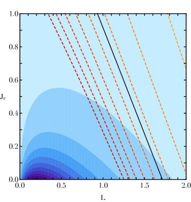
Figure 1: Illustration of the reduced DF, ${F(\mathbf{J})}$, as defined in Eq. (2), for an isotropic isochrone cluster, in units ${G\!=\!M\!=\!b_{\mathrm{c}}\!=\!1}$. Blue contours are spaced linearly between 5% and 95% of the function maximum. Dashed contours represent the level lines of the resonance frequency ${\omega\!=\!\mathbf{n}\!\cdot\!\mathbf{\Omega}(\mathbf{J})}$, for ${\mathbf{n}\!=\!(1,-1)}$. Contours are spaced linearly between ${\omega\!=\!0.04\,\Omega_{0}}$ (dark color) and ${\omega\!=\!0.005\,\Omega_{0}}$ (light color). As such the strong ${\ell\!=\!1}$ self-gravitating amplification, that occurs for ${\omega\!\simeq\!0.017\,\Omega_{0}}$ (black line, see also Fig. 3), can only resonantly couple to a very poorly populated location of action space, hence the inefficiency of collective effects to accelerate the RR relaxation (§3.2).

Other details of the model are given in §G.

In order to test Eq. (4) and the associated kinetic theories, we will now compare the NR and RR predictions to direct measurements in $N$-body simulations. In addition, in order to better highlight the importance of long-range couplings, we will consider two sets of clusters, either driven by the traditional Newtonian interaction, or by a softened Plummer interaction. Before diving into this comparison, a bit more work is required.

3.1 Curing divergences

First, as both NR and RR theories describe the dynamics of perturbations at linear order, e.g., through the linearised Vlasov equation, they both suffer from divergences associated with strong interactions (i.e. interactions at very short lengthscales). The NR theory also diverges at large scales. We now show how the various divergences may be cured.

3.1.1 NR relaxation and Coulomb logarithm

One drawback of the orbit-averaged FP theory is that it exhibits two divergences: one arising from stellar encounters with very small impact parameters, and one from encounters with very large impact parameters. As a result, the final answer, ${\mathbf{F}_{\mathrm{NR}}(\mathbf{J})}$, is necessarily proportional to the Coulomb logarithm

$$\ln\Lambda=\ln(b_{\mathrm{max}}/b_{\mathrm{min}})\,,$$ (11)

in which the minimum/maximum impact parameters $b_{\mathrm{min}/\mathrm{max}}$ have to be prescribed by hand. The first of these is traditionally taken to be the scale of $90^{\circ}$ deflections, ${2G\mu/\sigma^{2}}$, in the case of purely Newtonian interaction) or by the considered softening length $\varepsilon$ (as in Eq. (99)) for a softened interaction:

$$b_{\mathrm{min}}=\begin{cases}\displaystyle\frac{2G\mu}{\sigma^{2}}&\text{(Newtonian interaction)},\\[4.30554pt] \displaystyle\varepsilon&\text{(Softened interaction)},\end{cases}$$ (12)

with $\sigma$ the cluster’s velocity dispersion. Meanwhile, the maximum impact parameter is normally taken to be roughly the scale of the system itself; a reasonable choice is

$$b_{\mathrm{max}}\sim b_{\mathrm{c}},$$ (13)

with $b_{\mathrm{c}}$ the typical lengthscale of the considered cluster (e.g., the lengthscale entering the isochrone potential, see Eq. (104)). Of course, one should already be suspicious that interactions on these lengthscales do not satisfy the key assumptions of Chandrasekhar’s theory (see the Introduction), as they cannot seriously be considered either local or impulsive.

In practice, for the particular case ${N\!=\!10^{5}}$, and the parameters considered in our numerical simulations (see §H) we readily find from Eqs. (128) and (132) that the classical Coulomb logarithm reads

$$\ln\Lambda\simeq\begin{cases}\displaystyle 8.69&\text{(Newtonian interaction)},\\[4.30554pt] \displaystyle 3.60&\text{(Softened interaction)}.\end{cases}$$ (14)

As a result, for such a large value of $N$, strong encounters are drastically suppressed by softening, hence slowing down the evolution by a factor ${\sim\!2}$.

3.1.2 RR and divergence at small scales

In the RR theory, the spatial scale of each interaction is essentially set by the harmonic number $\ell$ (see §4.2 for further discussion). Because of this, the resonant flux $\mathbf{F}_{\mathrm{RR}}$ does not suffer from a large-scale divergence: the largest scales in the problem are set by the minimum harmonic number ${\ell=0}$ from which there stems a finite contribution. However, $\mathbf{F}_{\mathrm{RR}}$ still exhibits a small-scale divergence, associated with ${\ell\!\to\!+\infty}$ and the improper accounting of hard interactions, that one must heuristically cure. We now explore how this divergence arises, and offer a prescription for dealing with it in practice.

We first note that, all things being equal, from the prefactor of Eq. (10) we expect the flux $\mathbf{F}_{\mathrm{RR}}^{\ell}$ to be proportional to ${1/\ell}$ for large $\ell$, a scaling already noticed by Weinberg (1986) in the context of resonant dynamical friction. At this point one might argue that the presence of the coefficient ${|\Lambda^{\ell}_{\mathbf{n}\mathbf{n}^{\prime}}|^{2}}$ may change this simple picture; however, in practice it turns out that ${\mathbf{F}_{\mathrm{RR}}^{\ell}\!\propto\!1/\ell}$ is a good relation. We confirm this prediction numerically in Fig. 2 for the particular case of the spherical isochrone potential. In this figure, we plot the value of the resonant flux $|\mathbf{F}_{\mathrm{RR}}^{\ell}|$ at a particular phase space location $\mathbf{J}$ as a function of $\ell$.

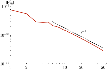
Figure 2: Illustration of the respective contributions from a given harmonic $\ell$ to the resonant flux from Eq. (9), in the absence of collective effects, in units ${G\!=\!M\!=\!b_{\mathrm{c}}\!=\!1}$. Here, the RR flux has been computed at the orbital location ${(J_{r},L)\!=\!(0.1,0.5)}$, with ${0\!\leq\!\ell\!\leq\!50}$, and ${|n_{1}|,|n^{\prime}_{1}|\leq 200}$, using ${K\!=\!500}$ points to compute the orbit-average, and ${K_{\mathrm{res}}\!=\!500}$ points to construct the resonance lines. For ${\ell\!=\!50}$, this amounts to considering more than $10^{8}$ resonance pairs ${(\mathbf{n},\mathbf{n}^{\prime})}$ possibly contributing to the flux. For ${\ell\!\gtrsim\!6}$, we recover ${|\mathbf{F}_{\mathrm{RR}}^{\ell}|\!\propto\!1/\ell}$, i.e. the logarithmic divergence on small scales associated with the unsoftened Newtonian interaction.

(To understand how we computed $\mathbf{F}_{\mathrm{RR}}^{\ell}$, itself a significant technical challenge, see §E–G). We see that for the purely Newtonian interaction, we find the expected scaling ${|\mathbf{F}_{\mathrm{RR}}^{\ell}|\!\propto\!1/\ell}$ for ${\ell\!\gtrsim\!\ell_{\mathrm{crit}}\!\equiv\!6}$. This scaling naturally leads to a logarithmic divergence in the calculation of the RR flux, since for $\ell_{\mathrm{max}}$ large enough, one has ${\sum_{\ell=0}^{\ell_{\mathrm{max}}}\!1/\ell\!\propto\!\ln(\ell_{\mathrm{max}})}$. We also point out that, for a fixed $\ell$, there is no divergence of Eq. (9) w.r.t. the infinite sum ${\sum_{\mathbf{n},\mathbf{n}^{\prime}}}$, as illustrated in Fig. 13. The problem is therefore to choose the ${\ell_{\mathrm{max}}}$ at which the infinite harmonic sum from Eq. (9) should be truncated.

To find the appropriate $\ell_{\mathrm{max}}$, we first note that the efficiency of resonant interactions is determined by the coupling coefficients ${\Lambda_{\mathbf{n}\mathbf{n}^{\prime}}^{\ell}}$. For large $\ell$ we expect collective amplification to be unimportant as high frequency oscillations cancel out long-range effects (see Fig. 4), so we consider only the bare coefficients defined in Eq. (86). From Eq. (85) we know that the efficiency of the coupling between two locations $r$ and $r^{\prime}$ is proportional to

$$U_{\ell}(r,r^{\prime})\propto\frac{1}{r_{\mathrm{max}}}\,\bigg{(}\!\frac{r_{\mathrm{min}}}{r_{\mathrm{max}}}\!\bigg{)}^{\ell},$$ (15)

with ${r_{\mathrm{min}}\!=\!\min(r,r^{\prime})}$ and ${r_{\mathrm{max}}\!=\!\max(r,r^{\prime})}$. As $\ell$ increases, this function gets sharper so that only very local interactions get picked up by the resonant interaction. Let us then consider one such interaction in the core of the cluster, and let us take ${r_{\mathrm{max}}\!=\!b_{\mathrm{c}}}$ (the typical lengthscale of the cluster’s density), and ${r_{\mathrm{min}}\!=\!b_{\mathrm{c}}(1\!-\!\alpha)}$, with ${\alpha\!>\!0}$. For two stars to have a close encounter necessarily requires that $\alpha$ is very small. Therefore in the limit of interest (${\alpha\!\ll\!1,\ell\!\gg\!1}$), Eq. (15) becomes

$$U_{\ell}(\alpha)\propto\frac{1}{b_{\mathrm{c}}}\,\big{(}1\!-\!\alpha\big{)}^{\ell}\simeq\frac{1}{b_{\mathrm{c}}}\,\mathrm{e}^{-\ell\alpha}.$$ (16)

The typical separation associated with this interaction is that given by its half-width, i.e. the value of $\alpha$ such that ${U_{\ell}(\alpha)/U_{\ell}(0)\!=\!\tfrac{1}{2}}$. One naturally gets ${\alpha\!=\!\ln(2)/\ell}$. For a given harmonic $\ell$, ${b_{\mathrm{c}}\alpha}$ then corresponds to the smallest scale of separation that is effectively resolved by the coupling coefficients. As a consequence, equating this interaction scale with $b_{\mathrm{min}}$, we may then truncate the RR harmonics expansion at

$$\ell_{\mathrm{max}}=\ln(2)\,\frac{b_{\mathrm{c}}}{b_{\mathrm{min}}},$$ (17)

hence heuristically curing the small-scale divergence of the RR theory.

For the parameters considered in our numerical simulations, (see §H), we therefore truncate the RR flux computation at

$$\ell_{\mathrm{max}}\simeq\begin{cases}\displaystyle 4115&\text{(Newtonian interaction)},\\[4.30554pt] \displaystyle 25&\text{(Softened interaction)}.\end{cases}$$ (18)

We note that the introduction of softening strongly reduces the range of harmonics that contribute to the dynamics.

3.2 The role of collective effects in RR

A central feature of the BL formalism is that it accounts for the collective amplification (‘dressing’) of potential fluctuations. Mathematically, this amplification is captured in the RR flux from Eq. (10) through the frequency-dependent dressed coupling coefficients ${\Lambda_{\mathbf{n}\mathbf{n}^{\prime}}^{\ell}(\mathbf{J},\mathbf{J}^{\prime},\omega)}$, which are defined in Eq. (78). These coefficients in turn depend on the susceptibility matrix ${\mathbf{N}_{\ell}(\omega)}$, defined in Eq. (46). If one ignores collective effects then ${\mathbf{N}_{\ell}(\omega)\!\to\!\mathbf{I}}$, the dressed coupling coefficients become the bare coupling coefficients (§F.1), and the BL flux reverts to the Landau flux.

It is natural to ask what impact the collective amplification has upon secular evolution in spherical systems — in other words, how does the BL prediction differ from that of Landau? In this section we argue that the difference between BL and Landau predictions is marginal on the largest scales, and is otherwise negligible, so that collective effects have only a minor role to play in the bulk evolution of dynamically hot stellar systems.

To see this, we begin by considering the top panel of Fig. 3, in which we plot the eigenvalue of ${\mathbf{N}_{\ell}(\omega)}$ that has the greatest modulus, which we call $|\lambda|_{\mathrm{max}}$, as a function of $\omega$ for different $\ell$.

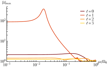
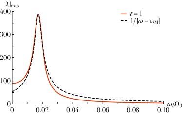
Figure 3: Top panel: Illustration of the maximum eigenvalue norm, ${|\lambda(\omega)|_{\max}}$, of the susceptibility matrix, ${\mathbf{N}_{\ell}(\omega)}$, as a function of the frequency $\omega$, and for various harmonics $\ell$. Both axes are logarithmic. Bottom panel: Same as the top panel except on linear axes, and zoomed around the frequency of the ${\ell\!=\!1}$ weakly damped mode, along with a function ${\!\propto\!1/|\omega\!-\!\omega_{\mathrm{M}}|}$. As already put forward in Weinberg (1994), globular clusters generically support a weakly damped ${\ell\!=\!1}$ mode, here estimated with the complex frequency ${\omega_{\mathrm{M}}/\Omega_{0}\!\simeq\!0.017\!-\!0.0024\,\mathrm{i}}$, using the peak’s position and full width at half maximum. The BL equation accounts for the amplification of fluctuations at all real frequencies, and naturally the biggest effect is around that frequency, leading to a very efficient self-gravitating dressing of the perturbations. Yet, such a low frequency is only commensurate with outer orbits in the cluster, hence the inefficiency of collective effects to accelerate the RR relaxation in the centre of the cluster. See §B.2 for the details of the numerical parameters used.

Clearly, if collective amplification is to be an important effect (i.e. if ${\mathbf{N}_{\ell}(\omega)}$ is to differ significantly from $\mathbf{I}$) for any given $\ell$ and $\omega$, then this eigenvalue must differ significantly from unity. We see from the plot that in all cases, ${|\lambda|_{\mathrm{max}}\to 1}$ for $|\omega/\Omega_{0}|\gtrsim 1$, meaning collective effects are unimportant at high frequencies. Meanwhile ${|\lambda|_{\mathrm{max}}\!\gg\!1}$ is achievable for ${\ell\!=\!1}$, i.e. dipole fluctuations can be greatly enhanced by collective amplification (Weinberg, 1994; Lau & Binney, 2019; Heggie et al., 2020). However, even for ${\ell\!=\!1}$ the amplification is large (${|\lambda|_{\mathrm{max}}\!\gtrsim\!10}$) only for very small frequencies, ${\omega/\Omega_{0}\!\lesssim\!0.1}$. In the lower panel of Fig. 3 we demonstrate that the ${\ell\!=\!1}$ curve exhibits a clear and narrow amplification around the frequency ${\omega\!\simeq\!0.017\,\Omega_{0}}$. This peak is to be interpreted as the imprint along the real frequency line of the cluster’s ${\ell\!=\!1}$ weakly damped mode (Weinberg, 1994), i.e. a pole of the susceptibility matrix, ${\mathbf{N}_{\ell=1}(\omega)}$, in the lower half of the complex frequency plane. More precisely, following Eq. (139) of Nelson & Tremaine (1999), it is sensible to approximate

$${|\lambda(\omega)|_{\max}\,\propto\,1/|\omega\!-\!\omega_{\mathrm{M}}|},$$ (19)

around this peak, where $\omega_{\mathrm{M}}$ is the complex frequency of the mode, with ${\mathrm{Im}[\omega_{\mathrm{M}}]\!<\!0}$. By fitting the analytical form from Eq. (19) to match the amplitude and full-width half-maximum of our numerical results, we estimate ${\omega_{\mathrm{M}}/\Omega_{0}\!\simeq\!0.017\!-\!0.0024\,\mathrm{i}}$. To summarise, the dressed coupling coefficients ${\Lambda_{\mathbf{n}\mathbf{n}^{\prime}}^{\ell}(\mathbf{J},\mathbf{J}^{\prime},\omega)}$ may differ markedly from their corresponding bare ones only for ${\ell\!=\!1}$ and ${\omega/\Omega_{0}\!\lesssim\!0.1}$, and the strongest amplification will be centred on $\omega/\Omega_{0}\simeq 0.017$.

We can now use this information to pinpoint the likely impact of collective effects on the secular evolution. Considering again Eq. (10), we see that the coupling coefficients contribute to the flux ${\mathbf{F}_{\mathbf{n}\mathbf{n}^{\prime}}^{\ell}(\mathbf{J})}$ at the resonance frequency ${\omega\!=\!\mathbf{n}\!\cdot\!\mathbf{\Omega}}$. Moreover, we know from §E.1 that for ${\ell\!=\!1}$ the only vectors $\mathbf{n}$ that contribute are of the form ${\mathbf{n}\!=\!(n_{1},1)}$, with ${n_{1}\!\in\!\mathbb{Z}}$ any integer. Putting these two facts together with the requirement ${\omega/\Omega_{0}\!\lesssim\!0.1}$, we see that ${\mathbf{F}_{\mathbf{n}\mathbf{n}^{\prime}}^{\ell}(\mathbf{J})}$ may undergo significant collective amplification only if ${\ell\!=\!1}$, ${\mathbf{n}\!=\!(n_{1},1)}$, and

$$n_{1}\Omega_{1}+\Omega_{2}\lesssim 0.1\,\Omega_{0}.$$ (20)

Given that ${\Omega_{1},\Omega_{2}\!>\!0}$ and that orbits in cored spherical systems always have ${1/2\!\leq\!\Omega_{2}/\Omega_{1}\!\leq\!1}$, the only practical value of $n_{1}$ for which some stars will be capable of satisfying Eq. (20) is ${n_{1}\!=\!-1}$. This can be checked easily in the case of the isochrone potential, for which we have explicit expressions for the frequencies (§G), but should hold for all sensible cored spherical potentials. In Fig. 1 we plot contours of the reduced isotropic DF of the isochrone model, ${F(\mathbf{J})}$. Overplotted with dashed lines are contours of $|{(-1,1)\!\cdot\!\mathbf{\Omega}}|$ spaced linearly from a maximum of ${0.04\,\Omega_{0}}$ (dark) to a minimum of ${0.005\,\Omega_{0}}$ (light). Since ${\ell\!=\!1}$ fluctuations are amplified most strongly around ${\simeq\!0.017\,\Omega_{0}}$, we see that even for ${n_{1}\!=\!-1}$, the condition from Eq. (20) holds only in a very sparsely occupied region of action space.

To complete our argument, we look once again at Eq. (10). The Dirac delta function in its right hand side demands that a star with action $\mathbf{J}$ and frequency ${\mathbf{n}\!\cdot\!\mathbf{\Omega}}$ couples to another star with action $\mathbf{J}^{\prime}$ and frequency ${\mathbf{n}^{\prime}\!\cdot\!\mathbf{\Omega}^{\prime}}$ only if ${\mathbf{n}\!\cdot\!\mathbf{\Omega}\!=\!\mathbf{n}^{\prime}\!\cdot\!\mathbf{\Omega}^{\prime}}$. But for this interaction to be strongly amplified by collective effects, we require Eq. (20) to be true, which we have just seen means that ${F(\mathbf{J})}$ and ${F(\mathbf{J}^{\prime})}$ and their gradients are very small. This fact severely suppresses the flux from Eq. (10) at the locations where strong self-gravitating amplification is possible. Moreover, since there is nothing particularly special about the isochrone potential or its isotropic DF, these conclusions ought to hold for all sensible spherical systems even with mildly anisotropic DFs. However, in isotropic systems ${F_{\mathrm{tot}}\!=\!F_{\mathrm{tot}}(E)}$, we note that ${\mathbf{n}\!\cdot\!\partial F/\partial\mathbf{J}\!=\!(\mathbf{n}\!\cdot\!\mathbf{\Omega})\,\mathrm{d}F/\mathrm{d}E}$. Since ${\omega\!=\!\mathbf{n}\!\cdot\!\mathbf{\Omega}}$ needs to be very small for the coupling coefficients ${\Lambda_{\mathbf{n}\mathbf{n}^{\prime}}^{\ell}(\mathbf{J},\mathbf{J}^{\prime},\omega)}$ to be amplified significantly, an additional small factor necessarily enters the flux computation at these frequencies, further suppressing the effect.

To summarise: (i) In near-isotropic spherical clusters, the only potential fluctuations that are greatly amplified by collective effects are ${\ell\!=\!1}$ (dipole) fluctuations at very low frequencies. (ii) For ${\ell\!=\!1}$ the only resonance vector that allows meaningful coupling to these very low frequency fluctuations is ${\mathbf{n}\!=\!\pm(-1,1)}$. (iii) The only stars that can resonantly couple to these low frequency fluctuations are on rather loosely bound orbits, which are sparsely populated. (iv) Secular evolution occurs only if two such stars couple to one another, which at these positions in $\mathbf{J}$ space is exceedingly rare. Thus we conclude that there are simply not enough pairs of stars able to resonate with one another at sufficiently low frequency for the collective dressing to be dominant. Put another way, collective effects will have at most a marginal impact on the largest scales, and will be totally absent on smaller scales.

In order to test these claims, we compare in Fig. 4 the RR predictions for ${\partial F/\partial t}$ for different harmonics $\ell$, in the presence (i.e. BL; left column) and absence (i.e. Landau; centre column) of collective effects.

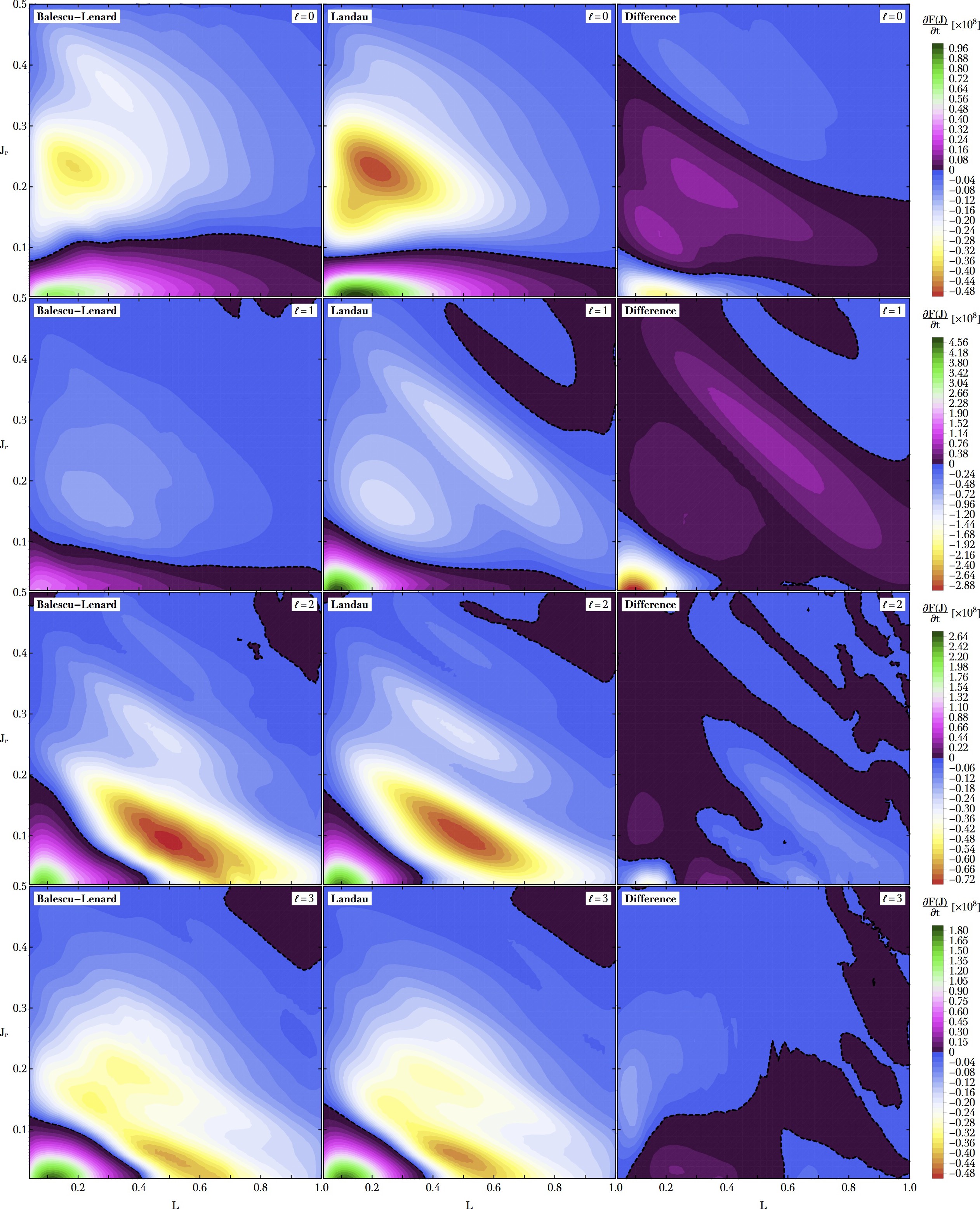
Figure 4: Illustration of the divergence of the RR diffusion flux, ${-\partial/\partial\mathbf{J}\!\cdot\!\mathbf{F}_{\mathrm{RR}}^{\ell}(\mathbf{J})\!=\!\partial F/\partial t}$, as defined in Eq. (9), in units ${G\!=\!M\!=\!b_{\mathrm{c}}\!=\!1}$, as a function of the considered harmonics $\ell$. The left panel corresponds to the dressed RR flux, as given by the BL equation, the centre panel is its bare analog given by the Landau equation, while the right panel corresponds to their differences. The number of orbits is predicted to increase in the central regions of action space, and decrease in the outer ones. We refer to §F for the numerical details. As expected, as $\ell$ increases, collective effects become less and less important. We also note that collective effects tend to decrease the efficiency of the RR relaxation, a paradoxical point already raised in Weinberg (1989).

In the right column we plot the difference between these two predictions (i.e. ‘BL minus Landau’). The numerical computations that give rise to this figure are highly non-trivial — for a discussion of their convergence, see §F.2. We note that the ${(L,J_{r})}$ range shown in Fig. 4 barely includes any of the resonance lines shown in Fig. 1, However, we emphasise that the action domain covered by Fig. 4 still contains about ${\sim 53\%}$ of the total mass of the cluster.

From the bottom two rows of Fig. 4 we see that for ${\ell\!=\!2,3}$ the impact of collective effects is already very small. Since self-gravity operates less efficiently on smaller scales, we can be confident that for ${\ell\!\geq\!\ell_{\mathrm{BL}}\!\equiv\!4}$, collective effects may be neglected completely (Weinberg, 1989). In other words, for ${\ell\!\geq\!\ell_{\mathrm{BL}}}$, we may use the Landau equation to safely compute the RR prediction for ${\partial F/\partial t}$. This greatly alleviates the numerical difficulty of future RR computations (§3.3), as it is far easier to compute the bare coupling coefficients ${\Lambda_{\mathbf{n}\mathbf{n}^{\prime}}^{\ell}}$ than the dressed ones — see §F.4.

Moreover, Fig. 4 shows us that even on the smallest scales ${\ell\!=\!0,1}$, the collective amplification is a marginal effect. Somewhat paradoxically, collective effects tend to reduce the efficiency of RR, in particular for ${\ell\!=\!0,1}$. Such a conclusion was already reached in Weinberg (1989) (see Fig. 7 therein), which showed that self-gravity tends to reduce the magnitude of the ${\ell\!=\!1}$ dynamical friction in spherical clusters. Such a trend was interpreted in Weinberg (1989) as being due to the fact that the self-gravitating wake generated by a perturber is symmetric and closely in phase with it, so that this wake cannot generate itself any significant torque back on the perturber. Interestingly, we note that for ${\ell\!=\!1}$, collective effects also lead to the fading of a diagonal ‘ridge’ that is present in the bare prediction, whereas, inversely, in self-gravitating discs, collective effects are what give rise to striking ridges in the action space diffusion map (Fouvry et al., 2015).

3.3 Computing the RR flux

In Fig. 2, we determined the critical harmonic number, ${\ell_{\mathrm{crit}}\!=\!6}$, at which the logarithmic scaling ${\mathbf{F}_{\mathrm{RR}}^{\ell}\!\propto\!1/\ell}$ starts to appear. In addition, in Eq. (18) we determined the maximum harmonic number $\ell_{\mathrm{max}}$ that must be considered in the infinite sum over harmonics. Of course for the sake of numerical feasibility, one can only estimate numerically the diffusion fluxes $\mathbf{F}_{\mathrm{RR}}^{\ell}$ for small enough values of $\ell$. In practice we are able to do this for ${\ell\!\leq\!\ell_{\mathrm{calc}}\!\equiv\!11}$. Such individual fluxes are illustrated in Fig. 5, in the absence of any collective effects.

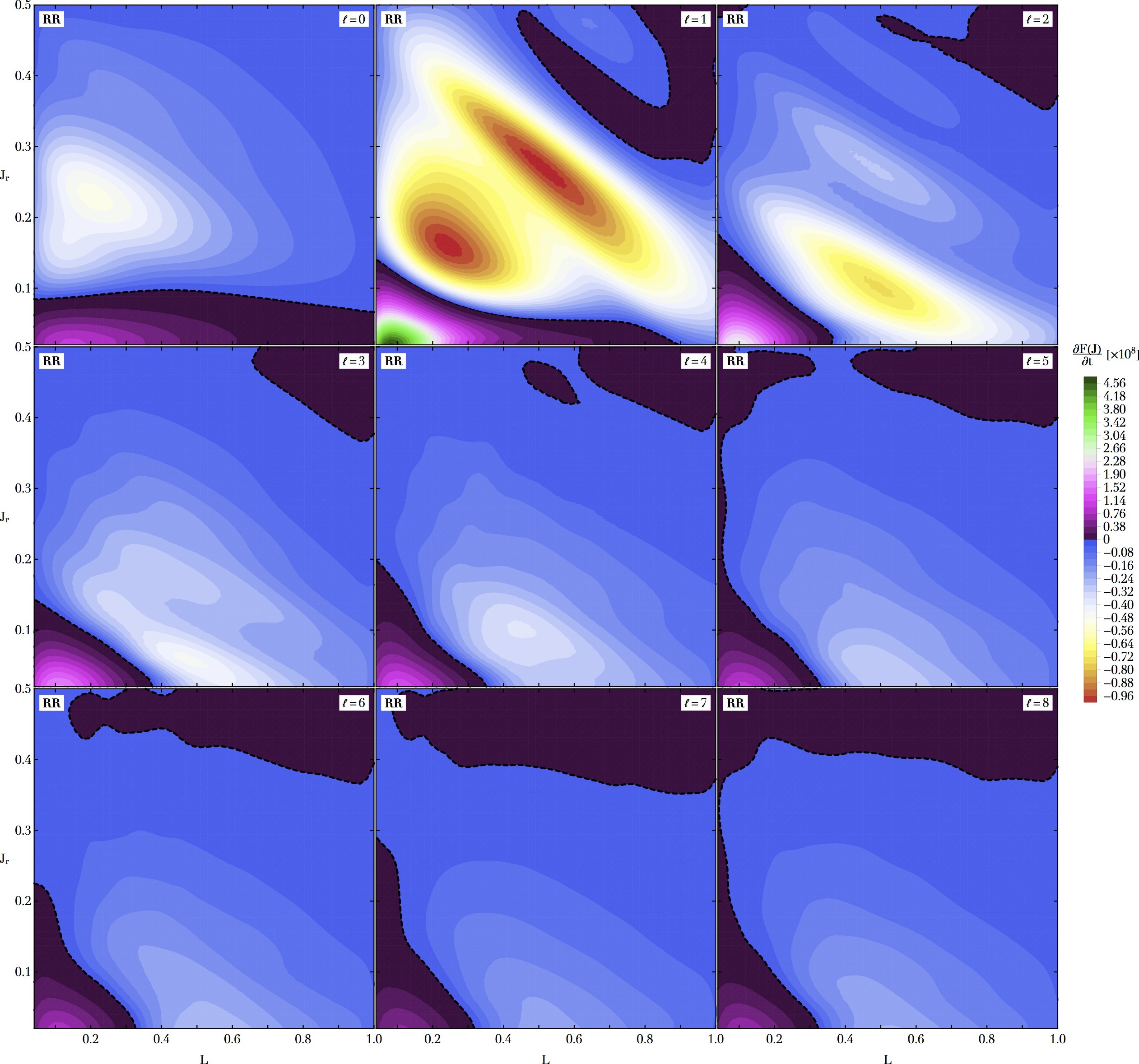
Figure 5: Illustration of the divergence of the bare (Landau) RR diffusion flux, ${-\partial/\partial\mathbf{J}\!\cdot\!\mathbf{F}_{\mathrm{RR}}^{\ell}(\mathbf{J})\!=\!\partial F/\partial t}$, as defined in Eq. (9), as a function of the considered harmonics $\ell$, without collective effects, using the same conventions as in Fig. 4. For $\ell$ large enough, the similarities in shape with the NR prediction presented in the central panel of Fig. 6 is striking.

Given these constraints, one may estimate the associated total RR diffusion flux as follows. To begin we decompose the flux into low- and high-order harmonic contributions:

$$\mathbf{F}_{\mathrm{RR}}{} =\mathbf{F}_{\mathrm{RR}}^{\mathrm{low}\,\ell}+\mathbf{F}_{\mathrm{RR}}^{\mathrm{high}\,\ell}$$ (21)

where

$$\mathbf{F}_{\mathrm{RR}}^{\mathrm{low}\,\ell}\equiv\sum_{\ell=0}^{\mathclap{\ell_{\mathrm{crit}}-1}}\mathbf{F}_{\mathrm{RR}}^{\ell};\quad\mathbf{F}_{\mathrm{RR}}^{\mathrm{high}\,\ell}\equiv\sum_{\mathclap{\ell=\ell_{\mathrm{crit}}}}^{\ell_{\mathrm{max}}}\mathbf{F}_{\mathrm{RR}}^{\ell},$$ (22)

We can now calculate these two contributions separately. For the low $\ell$ (i.e. large-scale) contribution, following Fig. 4 we have shown that for ${\ell\!\geq\!\ell_{\mathrm{BL}}\!=\!4}$, collective effects may be safely neglected. Thus we may approximate

$$\mathbf{F}_{\mathrm{RR}}^{\mathrm{low}\,\ell}\simeq\sum_{\ell=0}^{\mathclap{\ell_{\mathrm{BL}}-1}}\mathbf{F}_{\mathrm{RR}}^{\ell}[\mathrm{BL}]+\sum_{\mathclap{\ell=\ell_{\mathrm{BL}}}}^{\mathclap{\ell_{\mathrm{crit}}-1}}\mathbf{F}_{\mathrm{RR}}^{\ell}[\mathrm{Landau}],$$ (23)

i.e. collective effects are only accounted for for the harmonics ${0\!\leq\!\ell\!<\!\ell_{\mathrm{BL}}}$. Meanwhile for the high $\ell$ (i.e. smaller-scale) contribution, on account of the logarithmic scaling for ${\ell\!\gtrsim\!\ell_{\mathrm{crit}}}$, we can approximate

$$\mathbf{F}_{\mathrm{RR}}^{\mathrm{high}\,\ell}\simeq\kappa\sum_{\mathclap{\ell=\ell_{\mathrm{crit}}}}^{\ell_{\mathrm{calc}}}\mathbf{F}_{\mathrm{RR}}^{\ell},$$ (24)

where

$$\kappa \equiv\bigg{[}\sum_{\ell=\ell_{\mathrm{crit}}}^{\ell_{\mathrm{max}}}1/\ell\bigg{]}/\bigg{[}\sum_{\ell=\ell_{\mathrm{crit}}}^{\ell_{\mathrm{calc}}}1/\ell\bigg{]}.$$ (25)

$$=\begin{cases}\displaystyle 8.98&\text{(Newtonian interaction)},\\ \displaystyle 2.08&\text{(Softened interaction)}.\end{cases}$$ (26)

where we took ${\ell_{\mathrm{crit}}\!=\!6}$, and used the particular values of $\ell_{\mathrm{max}}$ from Eq. (18). The quantities on the right hand sides of Eqs. (23) and (24) are what we compute numerically. We get the total RR flux by summing them according to Eq. (21).

3.4 Comparing RR, NR and N-body evolution

We are now in a position to compare the NR and RR predictions with direct measurements from $N$-body simulations (see §H for the details of our numerical setup). Our main result is presented in Fig. 6, in which we plot contours of ${\partial F/\partial t}$ predicted by the NR (left) and RR theories (right) to those measured in $N$-body simulations (centre).

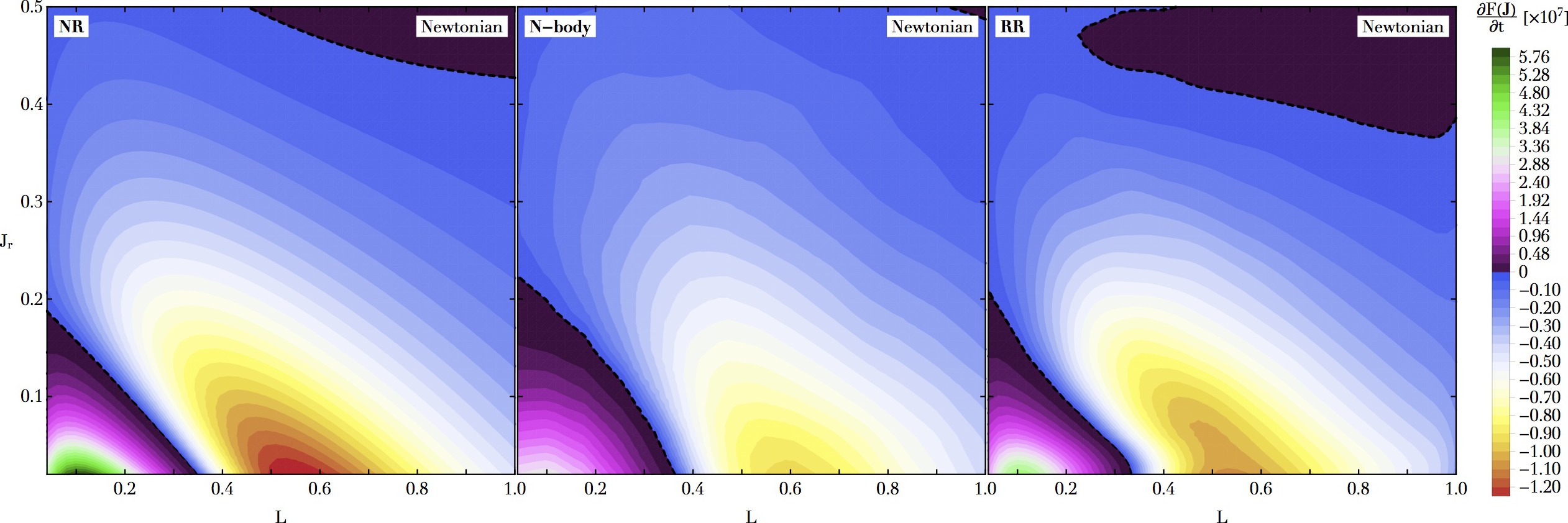
Figure 6: Illustration of the divergence of the diffusion flux, ${-\partial/\partial\mathbf{J}\!\cdot\!\mathbf{F}(\mathbf{J})\!=\!\partial F/\partial t}$, as predicted by the NR theory (left), measured in direct numerical simulations (centre), and predicted by the RR theory (right), using the same convention as in Fig. 4. The qualitative agreement between the three panels is striking. Note that the overall amplitude of NR is about twice that of the other panels.

While the shape of the contours differs slightly between each panel, it is reassuring to note that both NR and RR theories are in satisfactory agreement with $N$-body measurements. We note however that the NR theory over-estimates the efficiency of the relaxation by a factor ${\sim 2}$, which is reminiscent of an observation made by Theuns (1996). This amplitude mismatch is much reduced in the RR predictions. Of course, one should recall that the harmonic small-scale truncation from Eq. (17), and the associated self-similar summation from Eq. (21) still remain somewhat heuristic, and are likely responsible for some of the remaining mismatches present in Fig. 6.

The agreement between the $N$-body measurement on the one hand and the RR prediction on the other is a clear vindication of the BL/Landau kinetic theory. This is a non-trivial result, because implementing the BL/Landau formalism in practice involves significant technical challenges: as discussed above, it requires summing fluxes over many harmonics and extremely large numbers of resonances, which in turn requires very good accuracy for each contribution to the sum.

The relative match of the NR prediction with the numerical simulations comes as a pleasant surprise, since it is far simpler to implement than the RR theory. Yet, even if taken at face value, the NR prediction requires some significant tuning of ${\ln\Lambda}$ (by a factor $\sim{2}$) for which there exists no generic, effective and systematic prescription. In addition, it does raise some fundamental questions since the NR theory effectively ignores non-local resonances, which are properly accounted for by the RR theory. We further discuss all these elements in §4.

3.5 The impact of softening

Having investigated in the previous section the relaxation of a cluster governed by the Newtonian pairwise interaction, we now briefly turn our interest to the case of a softened interaction, as defined in Eq. (99). We refer to §H.2 for the details of our numerical setup.

In Fig. 7 we illustrate the impact of softening that cures the logarithmic divergence of the RR flux for ${\ell\!\to\!+\infty}$. (This result was already demonstrated in Fig. 5 of Weinberg (1986)).

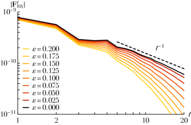
Figure 7: Same as in Fig. 2 but for a softened pairwise interaction, as in Eq. (99), with various softening lengths, $\varepsilon$. Here, we used ${0\!\leq\!\ell\!\leq\!20}$, and ${|n_{1}|,|n^{\prime}_{1}|\leq 40}$, using ${K\!=\!100}$ and ${K_{\mathrm{res}}\!=\!100}$. The larger the softening length, the more rapidly the flux contribution decays with $\ell$ for higher-order harmonics, as advocated in Eq. (103).

The larger $\varepsilon$, the stronger the softening, and therefore the stronger the dampening of the RR flux for large $\ell$, i.e. the smaller the contributions from small scales.

Following the prescriptions from Eqs. (14) and (18), we present in Fig. 8 the associated diffusion maps, as predicted by the NR and RR theories and measured in numerical (collisionless) simulations.

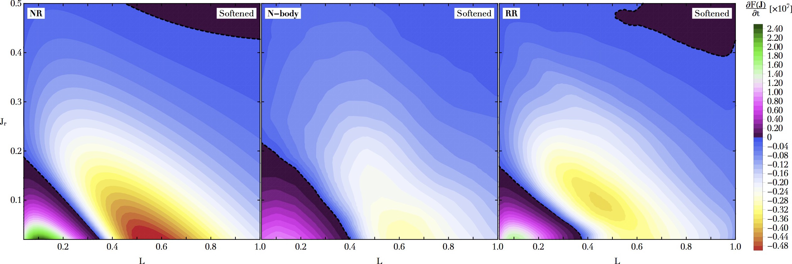
Figure 8: Same as in Fig. 6 but for a softened pairwise interaction with its respective prescriptions to deal with the NR and RR divergences.

As expected, we recover that the introduction of softening, because it smears out the contributions from small scales and hard encounters, leads to a reduction in the overall diffusion rate. Similarly to Fig. 6, we note that the NR theory still over-predicts the rate of relaxation by a factor ${\sim\!2}$. The RR kinetic theory presents once again a welcome satisfactory agreement with numerical simulations.

4 Discussion

Let us now discuss our results in steps: first the connection between RR and NR theories (§4.1), then how one may interpret our results in terms of orbit coupling (§4.2), how our results connect to those in previous works (§§4.3-4.4), and finally possible future extensions (§4.5).

4.1 From RR to NR

We recall that Fig. 5 shows the contribution to the Landau prediction for ${\partial F/\partial t}$ from harmonic $\ell$, namely ${-\partial/\partial\mathbf{J}\!\cdot\!\mathbf{F}_{\mathrm{RR}}^{\ell}}$, for ${\ell\!=\!0,...,8}$. One key result of this figure is that for ${\ell\!\gtrsim\!\ell_{\mathrm{crit}}\!=\!6}$, the map of ${-\partial/\partial\mathbf{J}\!\cdot\!\mathbf{F}_{\mathrm{RR}}^{\ell}}$ begins to resemble the NR prediction ${-\partial/\partial\mathbf{J}\!\cdot\!\mathbf{F}_{\mathrm{NR}}}$ (see the left panel of Fig. 6), up to an overall amplitude. In other words, the RR theory and the NR theory give qualitatively equivalent results on small scales. Heuristically, this may be understood as follows.

On the one hand, at large scales ${\ell\!\lesssim\!\ell_{\mathrm{crit}}}$, the pairwise coupling between orbits is not a very sharp function of their respective separation, as highlighted in Eq. (15). As a consequence, for such low-order harmonics, long-range resonant couplings are possible, leading to the non-trivial diffusion maps presented in the first panels of Fig. 5. We also recall that these maps maps are distorted by collective effects for the smallest $\ell$, as in Fig. 4, which the NR theory has no hope of accounting for.

On the other hand, for ${\ell\!\gtrsim\!\ell_{\mathrm{crit}}}$, the pairwise coupling becomes a sharp function of the stars’ separations. As a consequence, for such high-order harmonics, relaxation is made possible only through local scatterings, i.e. the form of relaxation captured by the NR theory from Eq. (5). As highlighted in the last panels of Fig. 5, this allows for the maps of $\mathbf{F}_{\mathrm{RR}}^{\ell}$ to greatly resemble the ones from $\mathbf{F}_{\mathrm{NR}}$ (see Fig. 5), up to an overall change in the amplitude, that follows the logarithmic scaling recovered in Fig. 2.

As such, one of the key improvements of the RR theory over the NR one is to offer a better estimation of the diffusion flux for low-order harmonics (i.e. the contributions from large scales). In addition, this inhomogeneous RR prediction also naturally cures the large-scale divergence present in the NR theory. While this does not significantly affect the overall structure of the maps of ${\partial F/\partial t}$, it does improve the estimation of the overall amplitude of the diffusion flux, as highlighted in Fig. 6.

Benefiting from this self-similarity between the NR theory and the large $\ell$ contribution to the RR theory, we may improve upon Eq. (21) and propose a simpler effective approach, combining both RR and NR, to estimate the total diffusion flux. As such, we write

$$\mathbf{F}=\mathbf{F}_{\mathrm{RR}}^{<\ell_{\mathrm{cut}}}+\mathbf{F}_{\mathrm{NR}}^{b_{\mathrm{cut}}}.$$ (27)

In that expression, the contribution from low-order harmonics, ${\mathbf{F}_{\mathrm{RR}}^{<\ell_{\mathrm{cut}}}}$, is computed as

$$\mathbf{F}_{\mathrm{RR}}^{<\ell_{\mathrm{cut}}}=\sum_{\ell=0}^{\mathclap{\ell_{\mathrm{cut}}-1}}\mathbf{F}_{\mathrm{RR}}^{\ell},$$ (28)

where, following Eq. (23), collective effects are also accounted for in low-order harmonics. In Eq. (27), we also introduced $\mathbf{F}_{\mathrm{NR}}^{b_{\mathrm{cut}}}$ as the NR flux computed with a Coulomb logarithm given by ${\ln\Lambda_{\mathrm{cut}}\!=\!\ln(b_{\mathrm{cut}}/b_{\mathrm{min}})}$, where the minimum impact parameter, $b_{\mathrm{min}}$, is given by Eq. (12), while the maximum impact parameter, $b_{\mathrm{cut}}$, is a function of $\ell_{\mathrm{cut}}$, and follows from Eq. (17) reading

$$b_{\mathrm{cut}}=\frac{\ln(2)}{\ell_{\mathrm{cut}}}\,b_{\mathrm{c}}.$$ (29)

Such an effective calculation is presented in Fig. 9, for both a Newtonian and softened interaction potential.

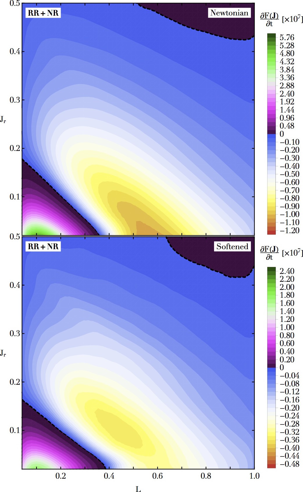
Figure 9: Same as Figs. 6 and 8 but using the effective diffusion flux from Eq. (27) that combines the RR and NR fluxes, for a Newtonian interaction (top) and a softened interaction (bottom), using a truncation at ${\ell_{\mathrm{cut}}\!=\!12}$. Accounting for the large-scale contributions to the flux using RR allows for an improved agreement with the numerical simulations, compared to the direct NR prediction.

In that figure, we note, on the one hand, that accounting for the large-scale contributions to the flux using RR rather than NR partially alleviates the amplitude mismatch that was observed in Figs. 6 and 8 when comparing the NR prediction with the numerical simulations. On the other hand, accounting for the small-scale contributions to the flux using NR rather than RR significantly alleviates the computational difficulty of the prediction, as one does not need to solve any non-local resonance condition, nor sum over numerous high-order resonance pairs. All in all, the effective approach from Eq. (27) appears as a promising way to effectively and simultaneously account for the joint effects of large-scale, resonant, dressed, and non-local contributions (as captured by RR), and small-scale, non-resonant, bare, and local contributions (as captured by NR).

4.2 Qualitative interpretation via orbit-orbit torques

Let us now attempt to explain the physical origin of the observed agreement between the RR and NR maps. The two basic questions we are trying to answer are as follows. (A) Why is it that the distinct conceptual pictures of (i) long-lived resonant encounters of stars with small scale potential fluctuations, and (ii) instantaneous local non-resonant two-body encounters between individual stars, ultimately end up being equivalent here? (B) Why do interactions of stars with small-scale (high $\ell$) potential fluctuations dominate the RR flux, rather than interactions with large-scale (low $\ell$) collectively dressed fluctuations?

To begin to answer these questions, let us start with (i) and argue why it is the same as (ii), at least for the system at hand. Let us also stress that in contrast to the result of the previous section, what follows in this sub section is only offered as a broad heuristic explanation that warrants further work. We shall ignore collective effects, since these are unimportant on small scales (see Fig. 4). Then the mathematical formalism behind (i) is Landau theory, i.e. with the same flux as in Eq. (10) but with the dressed coupling coefficients replaced by bare coefficients. We begin to make a connection with star-star scattering when we realise that the bare coupling coefficients entering the Landau flux are merely Fourier transforms of the interaction potential between pairs of stars w.r.t. both sets of angles (see, e.g., Pichon, 1994; Chavanis, 2013b). Concomitant with this, Rostoker’s principle (Gilbert, 1968; Hamilton, 2021) tells us that Landau theory is nothing more than a theory of bare two-body resonant interactions between stars on mean field orbits. Furthermore, we know that any star’s mean field orbit can be labelled by its ${3D}$ action ${\overline{\mathbf{J}}\!=\!(J_{r},L,L_{z})}$ and its ${3D}$ angle variable at some reference time, $\overline{\bm{\theta}}_{0}$, and then written as a Fourier series: ${\mathbf{r}(t)\!=\!\!\sum_{\overline{\mathbf{n}}}\!\mathbf{r}_{\overline{\mathbf{n}}}(\overline{\mathbf{J}})\exp(\mathrm{i}\overline{\mathbf{n}}\!\cdot\!\overline{\bm{\theta}})}$, with ${\overline{\bm{\theta}}\!=\!\overline{\bm{\theta}}_{0}\!+\!\overline{\mathbf{\Omega}}(\overline{\mathbf{J}})t}$. Taking this Fourier series literally, we could equivalently think of replacing each star on mean field orbit ${(\overline{\bm{\theta}}_{0},\overline{\mathbf{J}})}$ by a superposition of many (less massive) quasi-stars each labelled by $(\overline{\bm{\theta}}_{0},\overline{\mathbf{J}},\overline{\mathbf{n}})$, and having orbits ${\mathbf{r}(t)\!=\!\mathbf{r}_{\overline{\mathbf{n}}}(\overline{\mathbf{J}})\exp(\mathrm{i}\overline{\mathbf{n}}\!\cdot\!\overline{\bm{\theta}})}$. From this viewpoint the interaction between any two stars ${(\overline{\bm{\theta}}_{0},\overline{\mathbf{J}})}$ and ${(\overline{\bm{\theta}}_{0}^{\prime},\overline{\mathbf{J}}^{\prime})}$ can be thought of as a superposition of interactions between all possible pairs of quasi-stars labelled by $\overline{\mathbf{n}}$, $\overline{\mathbf{n}}^{\prime}$. Thus, Landau theory is a theory of bare interactions between all possible resonant quasi-stars. (Note that since we are now considering angles and actions in ${3D}$, we have not yet thrown away any information about the relative inclination of the orbital planes of these quasi-stars).

What sort of resonant interactions can pairs of quasi-stars have? To start with, given the corresponding ${2D}$ actions and resonant numbers in each corresponding plane $\mathbf{J}$, $\mathbf{J}^{\prime}$, $\mathbf{n}$ and $\mathbf{n}^{\prime}$ we can always find a rotating reference frame in which both quasi-star orbits are closed. As viewed in this reference frame there are then roughly four qualitative types of resonant interaction, stemming from the fact that the orbital orientations can be either ‘in-plane’ or ‘out-of-plane’, and that the resonances can be either ‘high-order’ or ‘low-order’. To illustrate what we mean, in the top two panels of Fig. 10, we show two typical quasi-star orbits in the isochrone potential, with ${\mathbf{n}\!=\!(-1,4)}$ in blue and ${\mathbf{n}^{\prime}\!=\!(1,4)}$ and in orange.

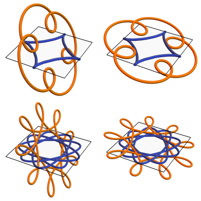
Figure 10: Illustration of the four basic types of interaction between quasi-star orbits with ${(J_{r},L)/\sqrt{GMb_{\mathrm{c}}}}$ equal to resp. ${(0.04,0.2)}$ (blue) and ${(0.11,0.4)}$ (orange). Roughly speaking we have (top left) out-of-plane interactions via a low-order resonance; (top right) close-to-in-plane interactions via a low-order resonance; (bottom left) out-of-plane interactions via a high-order resonance; (bottom right) close-to-in-plane interactions via a high-order resonance.

Note that we have transformed to the aforementioned rotating frame, so that both orbits are closed. On the top left we take the orbital planes to be inclined w.r.t. each other by an angle ${\pi/3}$, so that they are significantly ‘out-of-plane’. On the top right we have simply changed the relative angle to ${\pi/16}$ so that the two orbits are instead almost coplanar. Finally, the bottom panels show something similar except for a ‘higher-order’ resonance, namely taking ${\mathbf{n}\!=\!(-4,9)}$ (blue) and ${\mathbf{n}^{\prime}\!=\!(-2,9)}$ (orange).

Obviously, the ‘order’ of the resonance here corresponds roughly to the number of ‘loops’ in these diagrams. Thus, low-order resonances (top row) correspond to relatively small $\mathbf{n}$, $\mathbf{n}^{\prime}$ while high-order resonances correspond to relatively large ${\mathbf{n},\mathbf{n}^{\prime}}$ (bottom row). Moreover, as explained further in §D.2, the minimum relative inclination angle between quasi-star orbits is roughly set by ${\pi/\ell}$, so that large $\ell$ can capture near coplanar configurations (right) while small $\ell$ are limited to to out-of-plane interactions (left).

We can now plausibly answer question (A). Large $\ell$ means a typical small angular-scale ${\pi/\ell}$ between the two planes. Also, while there are very many high-order $\mathbf{n}$, $\mathbf{n}^{\prime}$ to choose from like in the bottom right panel of Fig. 10, there are not so many low-order ones like in the top right. Thus we expect the large-$\ell$ (small scale) contribution to the RR flux to mostly consist of interactions like those in the bottom right panel. These mimic local deflections: indeed, when the overlap between the two quasi-star orbits is strongest, the local trajectories follow paths as though they (locally) deflect one another. At this stage we already begin to suspect a similarity between (i) and (ii). Taking it a step further, the orbit-averaged NR theory assumes that the sequence of deflections can be considered as uncorrelated. The RR theory considers ${|n_{2}|\!\leq\!\ell}$ sequential deflections per azimuthal period in the rotating frame (see §E.1), and must be summed over many such $\ell$s (bottom-right panel of Fig. 10). Since the type of deflection decorrelates from one pair ${(\mathbf{n},\mathbf{n}^{\prime})}$ of orbital configurations to the next, it seems likely that the sum over such pairs in Eq. (9) induces the same level of decoherence as the a posteriori orbital average implemented in Eq. (7) for NR theory. Thus we end up with the heuristic expectation that the secular evolution predicted by large-$\ell$ RR theory behaves qualitatively the same as that predicted by NR theory.

To answer question (B), we ask more generally: which of the four configurations do we expect to dominate the secular evolution? We notice that there are simply not so many low values of $\ell$ to choose from, whereas the number of high $\ell$ is in principle infinite. Also, as we have seen, the value of $\ell$ puts a limit on the order of the resonance that may contribute to the RR flux, ${|n_{2}|,|n^{\prime}_{2}|\!\leq\!\ell}$, so that configurations like the bottom-left panel of Fig. 10 are rare. In addition to this, the lack of orbital overlap for low $\ell$ means that at a typical time in their mutual orbits the quasi-stars will typically be physically far apart, leading to rather weak interactions. Conversely, the large $\ell$ in-plane interactions (right panels in Fig. 10) allow for multiple localised overlaps, particularly from the numerous available high-order resonances (bottom right). This hand-waving argument suggests that the dominant contributions to the flux could come from many configurations like the bottom right panel, since they are strongest and most numerous.

When attempting to draw a closer connection to §3, recall that when $\ell$ is small, the interaction kernel ${U_{\ell}(r,r^{\prime})}$ is wide (see Eq. (85) and Appendix B.1), so that orbits can still couple at fairly different $r$ and $r^{\prime}$, whereas high-$\ell$ display a very narrow kernel. This is the basis-sampling counter-part to the geometric argument of ‘capturing in-and-out-of-plane orbit overlap’. If $\ell$ is large, a narrow kernel is sufficient to sample small local loops which can get close to each other in-plane; if $\ell$ is small the wider kernel accounts for the less locally-averaged impact of the other orbit: such terms will contribute to the sum, but, it turns out, less so. In fact, §3 showed that while contributions from ${\ell_{2}\!\gg\!\ell_{1}}$ are much smaller than that from $\ell_{1}$, i.e. ${\mathbf{F}_{\ell_{2}}\!\ll\!\mathbf{F}_{\ell_{1}}}$, each contribution from a decade ${\sum_{\ell=0.1\ell_{2}}^{10\ell_{2}}\!\!\mathbf{F}_{\ell}}$ is similar to any other decade ${\sum_{\ell=0.1\ell_{1}}^{10\ell_{1}}\!\!\mathbf{F}_{\ell}}$, in direct analogy with the NR case. It seems that the $\ell$-convergence of the kernel’s width in ${r/r^{\prime}}$ compensates the number of deflections set by the relevant patch of size ${\pi/\ell}$, so that each decade of $\ell$ contributes roughly the same amount to the flux (cf Fig. 2). In all likelihood, ${U_{\ell}(r,r^{\prime})}$ inherited this feature from the inverse-square law of the interaction, hence the same asymptotic ${1/\ell}$ contribution to the flux. Clearly this rough argument warrants further detailed exploration.

At this point one might also interject and argue that the interactions between quasi-stars ought not to be treated as bare Newtonian interactions at all, but rather as dressed by collective effects, i.e. mediated via the dressed coupling coefficients in Eq. (10). These collective effects will boost the contribution from the top-left-panel configurations (low $\ell$) for certain special pairs of small ${\mathbf{n},\mathbf{n}^{\prime}}$, and this will have some impact on the low $\ell$ flux. While this is true, the argument of §3.2 suggests that in hot isotropic spheres it is only a modest effect. A posteriori, our calculations of ${\partial F/\partial t}$ tell us that the low $\ell$ flux is insufficient to overwhelm the many contributions from configurations that look like the bottom-right panel.

Finally, we note that in this picture, the effect of softening as investigated in §3.5 acts as a minimum plane separation, effectively damping the divergent $1/\ell$ sum corresponding to the Coulomb logarithm, as observed in Fig. 7. More quantitatively, softening tends to make the interaction kernel ${U_{\ell}(r,r^{\prime})}$ flatter, so that when modulated by high-order resonances ${(\mathbf{n},\mathbf{n}^{\prime})}$ in $W_{\ell}^{\mathbf{n}\mathbf{n}^{\prime}}(\mathbf{J},\mathbf{J}^{\prime})$ in Eq. (87), it gives a vanishing contribution.

Overall, a geometric understanding of the quasi-star orbit-orbit coupling framework highlights a posteriori why the RR of spherical hot clusters can indeed quantitatively match the predictions of NR theory. A more quantitative analysis would require investigating the relative dressed populations of quasi-stars at each $\mathbf{n}$, $\mathbf{n}^{\prime}$, their relative ‘tumbling’ rates in the rotating frame, and so on. This is left for future work.

4.3 Relation to Hamilton et al. (2018)

Hamilton et al. (2018) applied the RR theory in the context of spherical stellar systems (i.e. globular clusters). The main aim of their paper was to evaluate the BL prediction for ${\partial F/\partial t}$ for the spherical isochrone potential, and then compare this to the Landau prediction (to evaluate the importance of collective effects for RR processes) and the Chandrasekhar prediction (to compare RR with the canonical NR theory). They performed this calculation for the same isotropic DF that we employed here (Eq. (54)), as well as for some anisotropic (but still stable) isochrone DFs. From the resulting maps of ${\partial F/\partial t}$, Hamilton et al. (2018) claimed the following: (i) collective amplification, particularly of ${\ell\!=\!1}$ fluctuations, is strong in spherical clusters so that the BL prediction for the relaxation rate is much larger than that of Landau; and (ii) the typical BL relaxation rate is comparable in magnitude to, or even greater than, the NR prediction of Chandrasekhar, while taking a very different form in $\mathbf{J}$-space. Based on these results, Hamilton et al. (2018) concluded that large-scale self-gravitating collective motions provide a crucial, and heretofore overlooked, contribution to the secular relaxation of globular clusters.

We would like to emphasise here that the formal results developed in the first four sections of Hamilton et al. (2018) are correct, and indeed we have based much of the present paper on those foundations. However, the remainder of Hamilton et al. (2018)’s results should be revised. (i) In §3.2 we gave an analytical argument for why collective amplification cannot be a dominant effect for the great majority of stars in a cored spherical cluster, at least without a strong velocity anisotropy. We justified this claim numerically in Fig. 4. In other words, at least in the great bulk of phase space there is no significant difference between the BL and Landau predictions of ${\partial F/\partial t}$. (ii) The RR and NR predictions are actually remarkably similar, once the contributions from high-order harmonics and resonances are correctly accounted for.

Why do the conclusions of Hamilton et al. (2018) differ so much from ours? The simple answer is that their numerical computations of ${\partial F/\partial t}$ were not converged. As in Fig. 11 here, Hamilton et al. (2018) verified their computation of the response matrix ${M_{pq}(\omega)}$ by recovering from it the ${\ell\!=\!2}$ radial orbit instability of Saha (1991). Their confidence in the accuracy of their code was strengthened by carrying out a detailed convergence study around this instability, showing its recovery did not depend on the code parameters beyond some threshold (see their Table 2). However, when they then came to computing ${\partial F/\partial t}$ for a stable ${F(\mathbf{J})}$ they eased the heavy computational burden by making three parameter truncations, none of which was truly justified. First, they considered only the largest scale fluctuations, namely those with ${\ell\!=\!0,1,2}$ — but as we illustrated in Fig. 2, ${\ell_{\max}\!=\!2}$ is definitely not sufficient to find any trace of the underlying small-scale logarithmic divergence inherent in the RR flux. Second, they truncated the sum over resonance vectors in Eq. (9) to ${|n_{1}|,|n^{\prime}_{1}|\!\leq\!2}$. As illustrated in Fig. 13, this is not satisfactory, as the contributions from high-order resonances are heavily under-estimated. Third, they computed the coupling coefficients ${\Lambda_{\mathbf{n}\mathbf{n}^{\prime}}^{\ell}}$ using a finite basis expansion with ${n_{\mathrm{cut}}\!=\!10}$ radial basis elements. While such a drastic truncation is sufficient to recover the large-scale ${\ell\!=\!2}$ mode (Fig. 11), it is not enough to resolve correctly the rest of the $\Lambda_{\mathbf{n}\mathbf{n}^{\prime}}^{\ell}$, as illustrated in Fig. 12.

4.4 Relations to other works

In recent decades, many authors have compared the predictions of Chandrasekhar’s theory of two-body relaxation to direct $N$-body experiments of spherical stellar clusters (e.g. Heggie & Hut, 2003; Vasiliev, 2015; Sellwood, 2015). Often, but not always, these studies have been geared towards describing the evolution of the system using an orbit-averaged FP equation in energy space (e.g., Vasiliev 2015 and references therein) or in energy-angular momentum space (e.g., Takahashi 1995; Drukier et al. 1999). There, the role of Chandrasekhar’s theory is to provide an estimate for the NR diffusion coefficients that enter the FP equation. The $N$-body experiments are needed (i) to check that the orbit-averaged FP theory is capable of describing the evolution at least qualitatively, and (ii) to make the description quantitative by calibrating the free parameter ${\ln\Lambda}$. These studies have found repeatedly that once ${\ln\Lambda}$ is fixed, NR theory does a remarkably good job of estimating the diffusion coefficients (Theuns, 1996) and therefore of determining secular evolution (Kim et al., 2008; e Silva et al., 2017), a finding corroborated by our Fig. 6. Moreover, the ‘free parameter’ ${\ln\Lambda}$ is often well-constrained, such that any two reasonable values of it can only produce NR relaxation rates that differ from one another in magnitude at the level of ${\!\sim\!10\%}$, and often less (Giersz & Heggie, 1994; e Silva et al., 2017).

Only occasionally has the agreement between NR theory and $N$-body simulation been called into question, except for systems that are rotating or that have strongly anisotropic DFs (see §4.5). Theuns (1996) measured diffusion coefficients in energy space using $N$-body simulations of King models, and compared these to the associated NR theoretical prediction. He found that while the agreement between the experimental diffusion coefficients and their NR theoretical counterparts is good, in King models that have low central concentration, the NR theory overestimates the diffusion rate by a factor ${\simeq 1.5\,\mbox{---}\,2}$. Noting that the isochrone model has low central concentration also, this finding is in agreement with what we found in Fig. 6 in a different setting. Theuns (1996) attributed this additional relaxation to collective effects (which should be accounted for by the BL formalism), or to the scattering of stars by global collective modes (which BL does not cover — see Hamilton & Heinemann 2020).

While these studies may be enough to convince one that NR theory is a sufficiently good workhorse for most practical purposes, they do not really probe in detail the underlying physics of relaxation. That is because they confine themselves to following the evolution of the cluster either in real space (looking at, e.g., the time-evolution of Lagrangian radii) or in the space of energies $E$. Important though these quantities are, they are imperfect for probing relaxation physics because changes in those quantities reflect adiabatic changes in the mean field. A key novel feature of the present study is that we calculated the secular evolution in the ${(J_{r},L)}$ action space, allowing us to separate true relaxation from the adiabatic evolution of the mean field potential ${\psi(r)}$ — whilst $E$ changes under slow changes in $\psi$, the actions ${(J_{r},L)}$ do not.

Other than the present paper, to our knowledge, the only study in which the action space evolution has been computed for a spherical stellar system from $N$-body experiments is Lau & Binney (2019). They performed $10^{4}$ brief $N$-body simulations of the isotropic isochrone cluster with ${N\!=\!10^{3}}$, and stacked their results to build up good statistics. They drew their initial conditions from a Poisson sampling of the underlying distribution ${F_{\mathrm{tot}}(E)}$. They showed very clearly that in the early stages of evolution, ${\ell\!=\!1}$ potential fluctuations are strongly amplified compared to the initial bare Poisson noise (c.f. our Fig. 3). This amplification had not yet saturated after ${\sim 3\,t_{\mathrm{cross}}}$ (where $t_{\mathrm{cross}}$ is a typical crossing time) which is when their simulations ended.

Lau & Binney (2019) then compared their results to the RR and NR predictions from Hamilton et al. (2018). However, as they acknowledged, the fact that the amplifying noise had not yet saturated meant that their simulations could not be considered a fair test of the BL theory, which assumes saturated noise from the outset. Our simulations do not suffer from this shortcoming because the larger $N$ value means that the dressing process has sufficient time to saturate before the system relaxes significantly. Moreover, $\mathbf{F}$ is a difficult quantity to measure in simulations. Indeed, it seems that Lau & Binney (2019) may actually have been measuring only the frictional contribution to $\mathbf{F}$, i.e. the part arising from the coefficient $\mathbf{D}_{1}$, rather than the full $\mathbf{F}$ (D. Heggie, private communication). Indeed, the flux measurement reported by Lau & Binney (2019) matches qualitatively the NR prediction for the frictional part of $\mathbf{F}$, as can be seen by comparing the middle panel of Fig. 11 of Lau & Binney (2019) with the upper panel of Fig. B1 of Hamilton et al. (2018).

In the present paper we chose to compute ${\partial F/\partial t}$ rather than the flux $\mathbf{F}$, because (i) one can measure it from $N$-body simulations in an unambiguous way and (ii) its theoretical value is insensitive to the addition of a $\mathbf{J}$-independent constant to the flux. In so doing we arrived at the conclusion that up to an overall scale factor the NR prediction for ${\partial F/\partial t}$ is remarkably similar to that measured in $N$-body experiments. While RR differs from NR at the largest scales, and while collective amplification may play some minor role in the RR prediction, like most classical studies we have concluded that relaxation does not differ fundamentally from the predictions of Chandrasekhar’s NR theory, at least in an isotropic cored globular cluster.

4.5 Future extensions

Of course, the present work is only a first step towards a complete description of the collective, long-range and resonant relaxation of globular clusters. Let us now list briefly several avenues that deserve further investigation.

First, for the sake of simplicity, we limited ourselves to only considering isotropic non-rotating clusters, i.e. clusters whose DF follows ${F_{\mathrm{tot}}\!=\!F_{\mathrm{tot}}(E)}$. As recently highlighted in Breen et al. (2017), clusters with (strong) tangential anisotropy can undergo a much more efficient relaxation. Accounting for anisotropic DFs, i.e. ${F_{\mathrm{tot}}\!=\!F_{\mathrm{tot}}(E,L)}$, would involve two main developments: (i) in the NR theory, as in Eq. (51), a computation of Rosenbluth potentials involving ${3D}$ integrals is necessary; (ii) in the RR theory, e.g., as highlighted in Rozier et al. (2019), clusters can support an ever stronger self-gravitating amplification, which may (or may not) lead to an efficient collective dressing of the low-order harmonics. All in all, understanding the secular relaxation of rotating spheres would be of genuine astrophysical interest: the set of possible resonances gets shifted by rotation, and stars can extract free energy from the mean rotation of the sphere. This may impact the importance of collective effects, especially at low $\ell$.

Second, the present investigation was limited to the case of an isochrone potential. It was picked for the convenience of offering an explicit angular mapping, as in Eq. (113), making the orbital averages numerically much more sound. Provided such explicit and well-behaved mappings can be designed, the present work could then naturally be extended to other cored potentials, as well as eventually cuspy ones. In addition, we limited ourselves to only computing the divergence of the diffusion flux at the initial time, ${t\!=\!0}$. It would be of interest to use the same kinetic theories to integrate forward in time the dynamics of ${F(\mathbf{J},t)}$, ideally up to the time of the cluster’s core collapse. Given the complexity of both the NR and RR formalisms, this will be no easy task.

Third, when computing the RR flux in Fig. 5, we emphasised that for $\ell$ large enough, the maps of ${-\partial/\partial\mathbf{J}\!\cdot\!\mathbf{F}_{\mathrm{RR}}^{\ell}}$ resemble those of ${-\partial/\partial\mathbf{J}\!\cdot\!\mathbf{F}_{\mathrm{NR}}}$, up to an overall amplitude. From the theoretical point of view, following §4.2 it would therefore be interesting to understand in detail how a global resonance condition between orbits, ${\delta_{\mathrm{D}}(\mathbf{n}\!\cdot\!\mathbf{\Omega}\!-\!\mathbf{n}^{\prime}\!\cdot\!\mathbf{\Omega}^{\prime})}$, as captured by the RR theory, formally falls back on the orbit-averaged contributions from local homogeneous deflections, as captured by the NR theory, provided that one considers large enough harmonics $\ell$, and large enough resonance numbers ${(\mathbf{n},\mathbf{n}^{\prime})}$. Similarly, one should also better understand the detailed origin of the scaling ${\mathbf{F}_{\mathrm{RR}}^{\ell}\!\propto\!1/\ell}$, observed in Fig. 2.

Fourth, while it is true that the BL equation captures the amplification, and that this amplification tends to be greatest when $\omega$ is close to the pattern frequency of a weakly damped normal mode of the stellar system, it does not account for the direct interaction between stars and this continuously excited damped mode, the subject of quasilinear (QL) theory (Rogister & Oberman, 1968; Hamilton & Heinemann, 2020). Weakly damped modes are weakly damped precisely because there are not many stars with which they resonate; hence, it may be expected that these QL interactions do not contribute much to the global evolution of $F$. However, their slow pattern speed means that they will interact resonantly with stars that are on large, long-period orbits and therefore only weakly bound to the system; hence possibly leading to excess evaporation beyond the two-body prediction (Hénon, 1960). Unfortunately, applying the QL operator in practice is no easy task as it first requires a detailed characterisation of the damped modes of a given cluster (Weinberg, 1994; Heggie et al., 2020) through the appropriate analytic continuation of linear response theory.

Finally, we emphasised here that the relaxation of a star’s ‘in-plane’ actions, i.e. ${\mathbf{J}\!=\!(J_{r},L)}$, up to a correction in the Coulomb logarithm, is mainly driven by local, small-scale contributions. Similarly, it would be of interest to determine whether or not the relaxations of the ‘out-of-plane’ actions, i.e. $\widehat{\mathbf{L}}$ the instantaneous orientation of the orbital plane, is also mainly driven by NR effects, or RR ones, following the steps of Meiron & Kocsis (2019); Fouvry et al. (2019).

5 Conclusion

The study of the secular relaxation of globular clusters has a long history dating back to Chandrasekhar (1943). It might come as a surprise that almost 80 years later, this topic of research should remain so active. While it has been claimed recently (Hamilton et al., 2018; Lau & Binney, 2019) that collective effects are able to greatly amplify the efficiency of cluster relaxation, our present work shows that for an isotropic isochrone sphere, Chandrasekhar’s orbit-averaged theory provides a good effective description, apart from an overall factor of ${\sim\!2}$ in the relaxation rate (Fig. 6). However, the physical basis of Chandrasekhar’s theory should not be taken entirely literally, since ‘collisions’ on the scale of the cluster are certainly neither impulsive nor local. Our implementations of both the NR and RR formalisms show that the dominant contribution to the fluxes arises from the decades of high $\ell$-harmonics. Interactions on these scales are barely affected by collective amplification. The collective amplification on the largest scales (low $\ell$-harmonics) are not totally negligible, but provide only a modest correction to the overall relaxation of such a dynamically hot sphere. From our softening analysis, we conclude that indeed the higher $\ell$-harmonics, i.e. small-scale perturbations, involving orbits captured in high-order resonances contribute most of the flux. Finally we presented a mixed NR and RR approach to effectively and simultaneously account for the joint effects of large scale, resonant, dressed, non-local contributions and small scale, non-resonant, bare, local contributions.

In future it will be of interest to extend our investigations to other cluster models. In particular, it is important to check how well our results hold for colder, thinner, rotating or anisotropic systems — in the rather extreme case of old razor-thin discs, Fouvry et al. (2015) have already shown that evolution is dominated by the RR processes driven by large-scale dressed fluctuations. One should also aim to better understand and characterise from the analytical point of view the deep connections between the NR and RR kinetic theories.

Data availability

The data and numerical codes underlying this article were produced by the authors. They will be shared on reasonable request to the corresponding author.

Appendix A Mean field dynamics

In this Appendix we spell out all our conventions to describe the mean field dynamics of a spherically symmetric ${3D}$ stellar system.

Following the notations from Tremaine & Weinberg (1984), we define the ${3D}$ angle-action coordinates as

$$\overline{\mathbf{J}}=(J_{r},L,L_{z}),$$ (30)

with the associated angles ${\overline{\bm{\theta}}\!=\!(\theta_{1},\theta_{2},\theta_{3})}$, and orbital frequencies ${\overline{\mathbf{\Omega}}\!=\!(\Omega_{1},\Omega_{2},0)}$. In that expression, $J_{r}$ is the radial action, $L$ the norm of the angular momentum vector, and $L_{z}$ its projection along a given $z$-direction. As a result of spherical symmetry ${\Omega_{3}\!=\!0}$, because mean field orbits remain within their orbital plane. The other two frequencies are given by

$$\frac{2\pi}{\Omega_{1}}{} =2\!\!\int_{r_{\mathrm{p}}}^{r_{\mathrm{a}}}\!\!\!\!\frac{\mathrm{d}r}{\sqrt{2(E-\psi(r))-L^{2}/r^{2}}},$$

$$\frac{\Omega_{2}}{\Omega_{1}}{} =\frac{L}{\pi}\!\!\int_{r_{\mathrm{p}}}^{r_{\mathrm{a}}}\!\!\!\!\frac{\mathrm{d}r}{r^{2}\sqrt{2(E-\psi(r))-L^{2}/r^{2}}},$$ (31)

where $r_{\mathrm{p}}$ (resp. $r_{\mathrm{a}}$) is the orbit’s pericentre (resp. apocentre). Once the orbit has been characterised, the position of the star is obtained through the angles

$$\theta_{1}{} =\!\!\int_{\mathcal{C}}\!\!\mathrm{d}r\,\frac{\Omega_{1}}{\sqrt{2(E-\psi(r))-L^{2}/r^{2}}},$$

$$\theta_{2}-\varphi{} =\!\!\int_{\mathcal{C}}\!\!\mathrm{d}r\,\frac{\Omega_{2}-L/r^{2}}{\sqrt{2(E-\psi(r))-L^{2}/r^{2}}},$$ (32)

where $\mathcal{C}$ is the contour going from the pericentre $r_{\mathrm{p}}$ up to the current position ${r\!=\!r(\theta_{1})}$, along the radial oscillation. The quantity $\varphi$ in Eq. (32) is the angle from the ascending node to the current location of the particle along the orbital motion — see Fig. 1 of Tremaine & Weinberg (1984).

As mentioned in §2 one can take advantage of the spherical symmetry of the problem and work exclusively with the in-plane angle-action coordinates. Thus we define

$$\mathbf{J}\equiv(J_{r},L);\quad\bm{\theta}\equiv(\theta_{1},\theta_{2});\quad\mathbf{\Omega}\equiv(\Omega_{1},\Omega_{2}).$$ (33)

Importantly, the shape of a mean field orbit is characterised by just two quantities, the actions $(J_{r},L)$. It will sometimes be more convenient instead to label orbits with the peri- and apocentre distances ${(r_{\mathrm{p}},r_{\mathrm{a}})}$, which are related to the energy $E$ and the angular momentum $L$ by

$$E=\frac{r_{\mathrm{a}}^{2}\,\psi(r_{\mathrm{a}})-r_{\mathrm{p}}^{2}\,\psi(r_{\mathrm{p}})}{r_{\mathrm{a}}^{2}-r_{\mathrm{p}}^{2}};\quad L=\sqrt{\frac{2(\psi(r_{\mathrm{a}})-\psi(r_{\mathrm{p}}))}{r_{\mathrm{p}}^{-2}-r_{\mathrm{a}}^{-2}}}.$$ (34)

One final way to label orbits, useful in numerical work, is via an effective semi-major axis and eccentricity defined as

$$a=\frac{r_{\mathrm{p}}+r_{\mathrm{a}}}{2};\quad e=\frac{r_{\mathrm{a}}-r_{\mathrm{p}}}{r_{\mathrm{a}}+r_{\mathrm{p}}}.$$ (35)

Such a rewriting proves particularly useful in Eq. (113) to perform numerically well-posed orbit-averages in the isochrone potential.

Appendix B Linear response theory

B.1 Basis method

In order to characterise the linear stability of a self-gravitating system, we follow the basis method (Kalnajs, 1976). We introduce a set of potentials and densities ${(\psi^{(\alpha)},\rho^{(\alpha)})}$ that satisfy the biorthogonality relation

$$\psi^{(\alpha)}(\mathbf{r})=\!\!\int\!\!\mathrm{d}\mathbf{r}^{\prime}\,U(\mathbf{r},\mathbf{r}^{\prime})\,\rho^{(\alpha)}(\mathbf{r}^{\prime}),$$

$$\!\!\int\!\!\mathrm{d}\mathbf{r}\,\psi^{(\alpha)*}(\mathbf{r})\,\rho^{(\beta)}(\mathbf{r})=-\delta_{\alpha\beta},$$ (36)

with ${U(\mathbf{r},\mathbf{r}^{\prime})\!=\!-G/|\mathbf{r}-\mathbf{r}^{\prime}|}$ the gravitational pairwise interaction. In the case of a spherical system, it is natural to write

$$\psi^{(\alpha)}(\mathbf{r}){} =Y_{\ell}^{m}(\vartheta,\phi)\,U_{n}^{\ell}(r),$$

$$\rho^{(\alpha)}(\mathbf{r}){} =Y_{\ell}^{m}(\vartheta,\phi)\,D_{n}^{\ell}(r),$$ (37)

with ${(r,\vartheta,\phi)}$ the usual spherical coordinates and $Y_{\ell}^{m}$ spherical harmonics normalised so that ${\!\int\!\mathrm{d}\vartheta\mathrm{d}\phi\sin\vartheta|Y_{\ell}^{m}(\vartheta,\phi)|^{2}\!=\!1}$. Equation (37) also involves the radial functions ${(U_{n}^{\ell},D_{n}^{\ell})}$, which we take to be real. As such, a given basis element is characterised by three integers: the label $\alpha$ is a shorthand for the triplet $(\ell,m,n)$ where ${\ell\!=\!0,1,2,...}$ and ${m\!=\!-\ell,-\ell+1,...,\ell}$ describe the angular dependence, and ${n\!\geq\!1}$ gives the radial dependence.

In practice, we use the radial basis elements from Clutton-Brock (1973). With our present convention, the radial functions of the basis elements read

$$U_{n}^{\ell}(r){} =A_{n}^{\ell}\,\frac{(r/R_{\mathrm{b}})^{\ell}}{(1+(r/R_{\mathrm{b}})^{2})^{\ell+1/2}}\,C_{n-1}^{(\ell+1)}(\rho),$$

$$D_{n}^{\ell}(r){} =B_{n}^{\ell}\,\frac{(r/R_{\mathrm{b}})^{\ell}}{(1+(r/R_{\mathrm{b}})^{2})^{\ell+5/2}}\,C_{n-1}^{(\ell+1)}(\rho).$$ (38)

In that expression, $R_{\mathrm{b}}$ is a fixed scale radius, and ${-1\!\leq\!\rho\!\leq\!1}$ is the rescaled variable

$$\rho=\frac{(r/R_{\mathrm{b}})^{2}-1}{(r/R_{\mathrm{b}})^{2}+1}.$$ (39)

Equation (38) also involves the Gegenbauer polynomials ${C_{n}^{(\alpha)}(\rho)}$. They can easily be computed through the upward stable recurrence relation

$$(n\!+\!1)C_{n+1}^{(\alpha)}\!(\rho)\!=\!2(n\!+\!\alpha)\rho\,C_{n}^{(\alpha)}\!(\rho)-(n\!+\!2\alpha\!-\!1)C_{n-1}^{(\alpha)}\!(\rho),$$ (40)

with the initial conditions

$$C_{0}^{(\alpha)}=1;\quad C_{1}^{(\alpha)}=2\alpha\rho.$$ (41)

Finally, in Eq. (38), we introduced the normalisation coefficients

$$A_{n}^{\ell}={} -\sqrt{G/R_{\mathrm{b}}}\,2^{2\ell+3}\,\ell!$$ (42)

$$\times{} \bigg{[}\!\frac{(n\!-\!1)!(n\!+\!\ell)}{(n\!+\!2\ell)!\big{[}4(n\!-\!1)(n\!+\!2\ell\!+\!1)\!+\!(2\ell\!+\!1)(2\ell\!+\!3)\big{]}}\!\bigg{]}^{1/2}\!\!,$$

as well as

$$B_{n}^{\ell}={} \frac{1}{\sqrt{G}\,R_{\mathrm{b}}^{5/2}}\,\frac{2^{2\ell+3}}{4\pi}\,\ell!$$ (43)

$$\times{} \bigg{[}\!\frac{(n\!-\!1)!(n\!+\!\ell)\big{[}4(n\!-\!1)(n\!+\!2\ell\!+\!1)\!+\!(2\ell\!+\!1)(2\ell\!+\!3)\big{]}}{(n\!+\!2\ell)!}\!\bigg{]}^{1/2}\!\!.$$

B.2 Response matrix

Having constructed basis elements, they may now be used to represent the potential fluctuations present in the system so as to characterise its linear stability. Following Eq. (37) of Hamilton et al. (2018), for a given harmonic $\ell$, the linear stability of a stellar cluster is characterised by the response matrix, ${\mathbf{M}_{\ell}(\omega)}$, with coefficients

$$M_{pq}^{\ell}(\omega)=\frac{2(2\pi)^{3}}{2\ell+1}\sum_{\mathclap{\begin{subarray}{c}n_{1}\\ |n_{2}|\leq\ell\\ (\ell-n_{2})\mathrm{even}\end{subarray}}}|y_{\ell}^{n_{2}}|^{2}{} \!\!\int\!\!\mathrm{d}\mathbf{J}\,L\,\frac{\mathbf{n}\!\cdot\!\partial F_{\mathrm{tot}}/\partial\mathbf{J}}{\omega-\mathbf{n}\!\cdot\!\mathbf{\Omega}(\mathbf{J})}$$

$$\times W_{\ell p}^{\mathbf{n}}(\mathbf{J})\,W_{\ell q}^{\mathbf{n}}(\mathbf{J}).$$ (44)

Here, ${y_{\ell}^{n}\!\equiv\!Y_{\ell}^{n}(\tfrac{\pi}{2},0)}$ are pure numbers, while (see Eq. (34) of Hamilton et al., 2018)

$$W_{\ell n}^{\mathbf{n}}(\mathbf{J})=\!\!\int_{0}^{\pi}\!\!\frac{\mathrm{d}\theta_{1}}{\pi}\,U_{n}^{\ell}(r)\,\cos\big{(}n_{1}\theta_{1}+n_{2}(\theta_{2}-\varphi)\big{)},$$ (45)

whose computation relies on the angle mappings from Eq. (32). Having computed the response matrix, we may finally define the susceptibility matrix as

$$\mathbf{N}_{\ell}(\omega)=\big{[}\mathbf{I}-\mathbf{M}_{\ell}(\omega)\big{]}^{-1}.$$ (46)

This matrix characterises the amplitude of the self-gravitating dressing of potential fluctuations, and is therefore involved in the dressed resonant diffusion flux (see Eq. (78)). In practice, for spherically symmetric systems the susceptibility matrix satisfies the symmetry

$$\mathbf{N}_{\ell}(-\omega_{\mathrm{R}})=\mathbf{N}_{\ell}^{*}(\omega_{\mathrm{R}}),$$ (47)

for ${\omega_{\mathrm{R}}\!\in\!\mathbb{R}}$, so that we only need to pre-compute the susceptibility matrix for ${\omega_{\mathrm{R}}\!\geq\!0}$.

B.3 Numerical computation

The most demanding computation in Eq. (44) is the computation of the coupling coefficients, ${W_{\ell n}^{\mathbf{n}}(\mathbf{J})}$, as defined in Eq. (45). In order to accelerate their evaluation, we follow an approach similar to the one of §B of Rozier et al. (2019).

First, as already introduced in Eq. (35), we label the orbits using ${(a,e)}$. To compute any integral, we follow the same trick as in Hénon (1971), and define an effective anomaly, ${-1\leq u\leq 1}$, through the explicit mapping

$$r(u)=a(1+ef(u))\quad\text{ with }\quad f(u)=u\big{(}\tfrac{3}{2}-\tfrac{1}{2}u^{2}\big{)}.$$ (48)

Doing so, any integral over $\theta_{1}$ can be rewritten as

$$\!\!\int_{0}^{\pi}\!\!\mathrm{d}\theta_{1}\,F{} =\!\!\int_{r_{\mathrm{p}}}^{r_{\mathrm{a}}}\!\!\!\!\mathrm{d}r\,\frac{\mathrm{d}\theta_{1}}{\mathrm{d}r}\,F=\!\!\int_{-1}^{1}\!\!\!\!\mathrm{d}u\,\frac{\mathrm{d}\theta_{1}}{\mathrm{d}r}\,\frac{\mathrm{d}r}{\mathrm{d}u}\,F,$$ (49)

where the Jacobian, ${\mathrm{d}\theta_{1}/\mathrm{d}r}$, naturally follows from Eq. (32). Following such a change of variables, integrands now have finite values at the edge of the integration domain. Furthermore, in order to increase the numerical stability of the scheme, we use an exact and well-posed expression for ${\mathrm{d}\theta_{1}/\mathrm{d}u}$, as presented in Eq. (113) for the specific case of the isochrone potential.

Following this rewriting, one could still naively interpret Eq. (45) as involving nested integrals, since one must also compute the values of ${\theta_{1}[u]}$ and ${(\theta_{2}\!-\!\varphi)[u]}$ following Eq. (32). Fortunately, we can use the same trick as in §B of Rozier et al. (2019) and interpret these joint integrals simply as the forward integration of a single 3-vector. This is the approach we pursued here. In practice, we used the traditional RK4 scheme (see, e.g., Press et al., 2007), using $K$ steps. Owing to the analytical expression from Eq. (113), the integrand is always numerically well-behaved, which prevents any issues at the boundaries of the integration where the radial velocity vanishes.

Having computed the coefficients ${W_{\ell n}^{\mathbf{n}}(\mathbf{J})}$, we now have at our disposal an efficient evaluation of the integrand from Eq. (44). In order to carry out the action integral present in that expression, we follow the same approach as in Fouvry et al. (2015) up to three main improvements. (i) The action space, $\mathbf{J}$, is remapped to the dimensionless coordinates ${(x,e)\!=\!(a/b_{\mathrm{c}},e)}$, with $b_{\mathrm{c}}$ the lengthscale of the considered isochrone model. It is within these coordinates that the orbital domain is tiled in small square regions of extension ${\Delta x\!\times\!\Delta e}$. (ii) In the expression of the approximated integrands, derivatives, such as ${\partial W_{\ell n}^{\mathbf{n}}/\partial x}$ and ${\partial W_{\ell n}^{\mathbf{n}}/\partial e}$, are not computed through finite differences but rather through their analytical expressions by computing explicitly the derivatives under the integral sign in Eq. (45). (iii) All angular integrals, including derivatives, are computed efficiently using the effective anomaly from Eq. (48) and the associated integration trick. Let us finally emphasise that, while Eq. (44) is a complicated function to compute, once evaluated, one can store pre-computed interpolation functions ${(\ell,p,q,\omega)\!\to\!N_{pq}^{\ell}(\omega)}$, which are then used to evaluate the dressed coupling coefficients from Eq. (78).

In order to validate our implementation of the response matrix, we set out to reproduce the radial-orbit instability of the isochrone potential recovered in Saha (1991), using the radially anisotropic DF from Eq. (115). This is illustrated in Fig. 11.

Figure 11: Illustration of the radial shape of the mode, ${\psi(r)}$, as measured in Fig. 4 of Saha (1991) and compared with the present method, for the unstable ${\ell\!=\!2}$ mode of the ${R_{\mathrm{a}}\!=\!b_{\mathrm{c}}}$ model. The normalisation of the vertical axis is arbitrary.

For these calculations, following Eq. (38), we considered a total of ${n_{\mathrm{max}}\!=\!20}$ basis elements with ${R_{\mathrm{b}}\!=\!5\,b_{\mathrm{c}}}$. In Eq. (44), the orbital integral was performed for ${\ell\!=\!2}$ using a uniform grid in ${(x,e)}$-space, with ${0\!\leq\!x\!\leq\!x_{\mathrm{max}}\!=\!10}$, ${0\!\leq\!e\!\leq\!1}$, with the step distances ${\Delta x\!=\!0.02}$, and ${\Delta e\!=\!0.002}$. In that same expression, the sum over resonances was limited to ${|n_{1}|\!\leq\!n_{1}^{\max}\!=\!10}$. Finally, the orbital averages in Eq. (45) were performed using ${K\!=\!100}$ steps.

In Fig. 11, we recover that the model ${R_{\mathrm{a}}\!=\!b_{\mathrm{c}}}$ supports an unstable mode with growth rate ${\eta\!\simeq\!0.0245\,\Omega_{0}}$ in good agreement with the value ${0.024\,\Omega_{0}}$ measured in Saha (1991). The radial shape of the unstable mode also offers a good agreement with Saha (1991). All in all, this shows the sanity of our present numerical implementation of the response matrix.

We use this matrix method in §3.2, in particular to understand the inefficiency of collective effects to enhance the RR relaxation in the core regions of isotropic clusters. In the numerical calculation presented in Fig. 3, we considered a total of ${n_{\mathrm{max}}\!=\!20}$ basis elements, using the basis from Eq. (38) with the scale radius ${R_{\mathrm{b}}\!=\!10\,b_{\mathrm{c}}}$. The sum over resonances was limited to ${|n_{1}|\!\leq\!n_{1}^{\max}\!=\!10}$, while the orbit-averages were performed with ${K\!=\!100}$ steps. Finally, the domain of orbital integration was limited to ${0\!\leq\!x\!\leq\!x_{\mathrm{max}}\!=\!20}$, ${0\!\leq\!e\!\leq\!1}$, with the uniform step distances ${\Delta x\!=\!0.02}$ and ${\Delta e\!=\!0.002}$.

Appendix C Fokker–Planck equation

In this Appendix, we detail our implementation of the orbit-averaged local diffusion coefficients that appear in the NR flux from Eq. (5). Here, we follow in particular calculations from Binney & Tremaine (2008) for the local velocity diffusion coefficients, and from Bar-Or & Alexander (2016) for the computation of the orbit-average.

Following Eq. (7.69) of Binney & Tremaine (2008), we write the traditional Fokker–Planck equation in velocity space with the convention

$$\frac{\partial P(\mathbf{v})}{\partial t}={} -\sum_{i=1}^{3}\frac{\partial}{\partial v_{i}}\big{[}\big{\langle}\delta v_{i}\big{\rangle}\,P(\mathbf{v})\big{]}$$

$$+\frac{1}{2}\sum_{i,j=1}^{3}\frac{\partial^{2}}{\partial v_{i}\partial v_{j}}\big{[}\big{\langle}\delta v_{i}\,\delta v_{j}\big{\rangle}\,P(\mathbf{v})\big{]},$$ (50)

where ${P(\mathbf{v})}$ stands for an arbitrary DF, proportional to the number of particles within the volume ${\mathrm{d}\mathbf{v}}$.

In a nutshell, the NR flux is computed through the following steps. (i) At a given phase space location ${(\mathbf{r},\mathbf{v})}$, one computes the local velocity diffusion coefficients, ${\langle\delta\mathbf{v}\rangle(\mathbf{r},\mathbf{v})}$ and ${\langle(\delta\mathbf{v})^{2}\rangle(\mathbf{r},\mathbf{v})}$, a calculation made easier by our assumption of an isotropic background DF. (ii) The local diffusion coefficients are translated into local diffusion coefficients in integrals of motion, in practice the energy and angular momentum, $E$ and $L$, e.g., via ${\langle\delta E\rangle(\mathbf{r},\mathbf{v})}$. (iii) Contributions from all these kicks accumulate as the star follows its mean field orbit, leading to the associated orbit-averaged diffusion coefficients, e.g., ${\langle\Delta E\rangle(\mathbf{J})\!=\!\!\oint\!\tfrac{\mathrm{d}\theta_{1}}{2\pi}\langle\delta E\rangle}$. (iv) Finally, the diffusion coefficients in $\mathbf{J}$-space are derived through the appropriate change of variables. Let us now be more specific for each of these steps.

The first- and second-order diffusion coefficients originate from local deflections. Following Eq. (7.83a) of Binney & Tremaine (2008), and paying a careful attention to our normalisation convention, for a single-mass cluster, they read

$$\big{\langle}\delta v_{i}\big{\rangle}{} =8\pi G^{2}\,\mu\ln\Lambda\,\frac{\partial h}{\partial v_{i}},$$

$$\big{\langle}\delta v_{i}\,\delta v_{j}\big{\rangle}{} =4\pi G^{2}\mu\ln\Lambda\,\frac{\partial^{2}g}{\partial v_{i}\partial v_{j}},$$ (51)

where we introduced ${\ln\Lambda}$ as the Coulomb logarithm. In practice, the Coulomb logarithm is fixed following the prescription from Eq. (11). In that expression, the Rosenbluth potentials are given by

$$h(\mathbf{r},\mathbf{v}){} =\!\!\int\!\!\mathrm{d}\mathbf{v}^{\prime}\,\frac{F_{\mathrm{tot}}(\mathbf{r},\mathbf{v}^{\prime})}{|\mathbf{v}-\mathbf{v}^{\prime}|},$$

$$g(\mathbf{r},\mathbf{v}){} =\!\!\int\!\!\mathrm{d}\mathbf{v}^{\prime}\,F_{\mathrm{tot}}(\mathbf{r},\mathbf{v}^{\prime})\,|\mathbf{v}-\mathbf{v}^{\prime}|.$$ (52)

For an isotropic DF, ${F_{\mathrm{tot}}(\mathbf{r},\mathbf{v})\!=\!F_{\mathrm{tot}}(r,v)}$, the diffusion coefficients are characterised by only three quantities, namely

$$\big{\langle}\delta v_{\parallel}\big{\rangle}{} \!=\!-2\kappa\!\!\int_{0}^{v}\!\!\mathrm{d}v^{\prime}\,\frac{v^{\prime 2}}{v^{2}}\,F_{\mathrm{tot}}(v^{\prime}),$$ (53)

$$\big{\langle}\big{(}\delta v_{\parallel}\big{)}^{2}\big{\rangle}{} \!=\!\frac{2}{3}\kappa\bigg{[}\!\!\int_{0}^{v}\!\!\mathrm{d}v^{\prime}\,\frac{v^{\prime 4}}{v^{3}}F_{\mathrm{tot}}(v^{\prime})+\!\!\int_{v}^{+\infty}\!\!\!\!\!\!\!\!\mathrm{d}v^{\prime}v^{\prime}F_{\mathrm{tot}}(v^{\prime})\bigg{]},$$

$$\big{\langle}\big{(}\delta v_{\perp}\big{)}^{2}\big{\rangle}{} \!=\!\frac{2}{3}\kappa\bigg{[}\!\!\int_{0}^{v}\!\!\!\!\mathrm{d}v^{\prime}\bigg{(}\!\frac{3v^{\prime 2}}{v}\!-\!\frac{v^{\prime 4}}{v^{3}}\!\bigg{)}F_{\mathrm{tot}}(v^{\prime})\!+\!2\!\!\int_{v}^{+\infty}\!\!\!\!\!\!\!\!\mathrm{d}v^{\prime}v^{\prime}F_{\mathrm{tot}}(v^{\prime})\bigg{]}.$$

where we introduced ${\kappa\!=\!16\pi^{2}G^{2}\mu\ln\Lambda}$, and did not write the dependence w.r.t. $r$ to shorten the expressions.

Fortunately, in the case of an isotropic DF, we can rewrite all these integrals as integrals over the energy. Noting that ${v\mathrm{d}v\!=\!\mathrm{d}E}$, we can rewrite Eq. (53) as

$$\big{\langle}\delta v_{\parallel}\big{\rangle}{} =-2\kappa\frac{1}{v}\,I^{\mathrm{inf}}_{1},$$

$$\big{\langle}\big{(}\delta v_{\parallel}\big{)}^{2}\big{\rangle}{} =\frac{2}{3}\kappa\bigg{[}I^{\mathrm{inf}}_{3}+I^{\mathrm{sup}}_{0}\bigg{]},$$

$$\big{\langle}\big{(}\delta v_{\perp}\big{)}^{2}\big{\rangle}{} =\frac{2}{3}\kappa\bigg{[}3I^{\mathrm{inf}}_{1}-I^{\mathrm{inf}}_{3}+2I^{\mathrm{sup}}_{0}\bigg{]},$$ (54)

where we introduced the one-dimensional integrals

$$I^{\mathrm{inf}}_{k}(r,v){} =\!\!\int_{\psi}^{E}\!\!\mathrm{d}E^{\prime}\,(v^{\prime}/v)^{k}\,F_{\mathrm{tot}}(E^{\prime}),$$

$$I^{\mathrm{sup}}_{k}(r,v){} =\!\!\int_{E}^{0}\!\!\mathrm{d}E^{\prime}\,(v^{\prime}/v)^{k}\,F_{\mathrm{tot}}(E^{\prime}).$$ (55)

In these expression, the boundary of the integrals are given by ${\psi\!=\!\psi(r)}$ and ${E\!=\!\tfrac{1}{2}v^{2}\!+\!\psi(r)}$. We also note that all orbits are taken to be bound, so that ${E,E^{\prime}<0}$. In practice, these integrals are computed using a midpoint rule with ${K\!=\!10^{3}}$ steps.

From these local diffusion coefficients in velocity, we can now compute the local diffusion coefficients in ${(E,L)}$. To do so, we rely on the relations ${E\!=\!\tfrac{1}{2}v^{2}\!+\!\psi(r)}$, and ${L\!=\!|\mathbf{r}\!\times\!\mathbf{v}|}$, that are perturbed to first order. Following Eqs. (85)–(89) in Bar-Or & Alexander (2016), we obtain

$$\big{\langle}\delta E\big{\rangle} {}=v\,\big{\langle}\delta v_{\parallel}\big{\rangle}+\frac{1}{2}\big{\langle}\big{(}\delta v_{\parallel}\big{)}^{2}\big{\rangle}+\frac{1}{2}\big{\langle}\big{(}\delta v_{\perp}\big{)}^{2}\big{\rangle},$$

$$\big{\langle}\delta L\big{\rangle}{} =\frac{L}{v}\big{\langle}\delta v_{\parallel}\big{\rangle}+\frac{r^{2}}{4L}\,\big{\langle}\big{(}\delta v_{\perp}\big{)}^{2}\big{\rangle},$$

$$\big{\langle}\big{(}\delta E\big{)}^{2}\big{\rangle}{} =v^{2}\big{\langle}\big{(}\delta v_{\parallel}\big{)}^{2}\big{\rangle},$$

$$\big{\langle}\delta E\,\delta L\big{\rangle}{} =L\,\big{\langle}\big{(}\delta v_{\parallel}\big{)}^{2}\big{\rangle},$$

$$\big{\langle}\big{(}\delta L\big{)}^{2}\big{\rangle}{} =\frac{L^{2}}{v^{2}}\big{\langle}\big{(}\delta v_{\parallel}\big{)}^{2}\big{\rangle}+\frac{1}{2}\bigg{(}r^{2}-\frac{L^{2}}{v^{2}}\bigg{)}\big{\langle}\big{(}\delta v_{\perp}\big{)}^{2}\big{\rangle}.$$ (56)

Having computed the local diffusion coefficients in ${(E,L)}$, we can now compute their orbit-average. For an isotropic system, it is given by the simple calculation

$$\big{\langle}\Delta E\big{\rangle}=\!\!\int_{0}^{\pi}\!\!\frac{\mathrm{d}\theta_{1}}{\pi}\,\big{\langle}\delta E\big{\rangle}.$$ (57)

In practice, to avoid any boundary issues, we use the exact same technique as in Eq. (49), and introduce an effective anomaly to perform the orbit-average. These integrals are then computed using a midpoint rule with ${K\!=\!10^{3}}$ steps.

At this stage, we have derived the orbit-averaged diffusion coefficients in ${(E,L)}$–space. It now only remains to translate them in the ${\mathbf{J}\!=\!(J_{r},L)}$ coordinates. Following Eqs. (122) and (123) of Bar-Or & Alexander (2016), under a coordinate transform of the form ${\mathbf{x}^{\prime}\!=\!\mathbf{x}^{\prime}(\mathbf{x})}$, the new diffusion coefficients are given by

$$\big{\langle}\Delta x^{\prime}_{k}\big{\rangle}{} =\frac{\partial x^{\prime}_{k}}{\partial x_{i}}\,\big{\langle}\Delta x_{i}\big{\rangle}+\frac{1}{2}\frac{\partial^{2}x^{\prime}_{k}}{\partial x_{i}\partial x_{j}}\,\big{\langle}\Delta x_{i}\Delta x_{j}\big{\rangle},$$

$$\big{\langle}\Delta x^{\prime}_{k}\Delta x^{\prime}_{l}\big{\rangle}{} =\frac{\partial x^{\prime}_{k}}{\partial x_{i}}\,\frac{\partial x^{\prime}_{l}}{\partial x_{j}}\,\big{\langle}\Delta x_{i}\Delta x_{j}\big{\rangle},$$ (58)

where the sums over $i$ and $j$ are implied. Fortunately, in the case of the isochrone potential, we have at our disposal an explicit expression for ${J_{r}\!=\!J_{r}(E,L)}$, as in Eq. (106), which eases this change of coordinates. Following all these manipulations, we finally obtain the first-order diffusion coefficient, ${\mathbf{D}_{1}(\mathbf{J})}$, and the second-order diffusion tensor, ${\mathbf{D}_{2}(\mathbf{J})}$, as in Eq. (5).

Appendix D Deriving the Balescu–Lenard flux

In this Appendix, we present the key steps of the derivation of the BL equation from the Klimontovich equation (Chavanis, 2012), focussing specifically on how, in spherically symmetric systems, the resulting ${3D}$ kinetic equation may rewritten as an effective ${2D}$ equation (Hamilton et al., 2018) involving a summation over $\ell$ harmonics.

D.1 From Klimontovich to Balescu–Lenard

The state of the globular cluster can be fully described by its discrete DF,

$$F_{\mathrm{d}}(\mathbf{x},\mathbf{v},t)=\sum_{i=1}^{N}\mu\,\delta_{\mathrm{D}}(\mathbf{x}-\mathbf{x}_{i}(t))\,\delta_{\mathrm{D}}(\mathbf{v}-\mathbf{v}_{i}(t)),$$ (59)

where ${(\mathbf{x}_{i}(t),\mathbf{v}_{i}(t))}$ stands for the location in phase space at time $t$ of particle $i$. For a given realisation, the dynamics of that DF is exactly described by the Klimontovich equation that takes here the short form

$$\frac{\partial F_{\mathrm{d}}}{\partial t}+\big{[}F_{\mathrm{d}},H_{\mathrm{d}}\big{]}=0,$$ (60)

where the Poisson bracket is defined with the convention

$$\big{[}f,h\big{]}=\frac{\partial f}{\partial\mathbf{x}}\!\cdot\!\frac{\partial h}{\partial\mathbf{v}}-\frac{\partial f}{\partial\mathbf{v}}\!\cdot\!\frac{\partial h}{\partial\mathbf{x}}.$$ (61)

In Eq. (60), we introduced the (specific) discrete Hamiltonian

$$H_{\mathrm{d}}(\mathbf{x},\mathbf{v},t)=\frac{1}{2}|\mathbf{v}|^{2}+\Phi_{\mathrm{d}}(\mathbf{x},t),$$ (62)

where the instantaneous potential, ${\Phi_{\mathrm{d}}\!=\!\Phi_{\mathrm{d}}[F_{\mathrm{d}}]}$, self-consistently depends on the system’s instantaneous DF, through the relation

$$\Phi_{\mathrm{d}}(\mathbf{x},t)=\!\!\int\!\!\mathrm{d}\mathbf{x}^{\prime}\mathrm{d}\mathbf{v}^{\prime}\,F_{\mathrm{d}}(\mathbf{x}^{\prime},\mathbf{v}^{\prime},t)\,U(\mathbf{x},\mathbf{x}^{\prime}),$$ (63)

with ${U(\mathbf{x},\mathbf{x}^{\prime})\!=\!-G/|\mathbf{x}\!-\!\mathbf{x}^{\prime}|}$ the Newtonian pairwise interaction.

We now assume that the system’s DF and potential can be decomposed into two components,

$$F_{\mathrm{d}}=F_{\mathrm{tot}}+\delta F;\quad H_{\mathrm{d}}=H_{\mathrm{tot}}+\delta\Phi,$$ (64)

such that ${\delta F\!\ll\!F_{\mathrm{tot}}}$ and ${\delta\psi\!\ll\!H_{\mathrm{tot}}}$. Perturbations are such that ${\langle\delta F\rangle\!=\!0}$, and ${\langle\delta\Phi\rangle\!=\!0}$, with ${\langle\,\cdot\,\rangle}$ the ensemble average over realisations. Importantly, we note that the DF’s and potential fluctuations are self-consistent as, similarly to Eq. (63), one has

$$\delta\Phi(\mathbf{x},t)=\!\!\int\!\!\mathrm{d}\mathbf{x}^{\prime}\mathrm{d}\mathbf{v}^{\prime}\,\delta F(\mathbf{x}^{\prime},\mathbf{v}^{\prime},t)\,U(\mathbf{x},\mathbf{x}^{\prime}).$$ (65)

We assume that the mean system is in an integrable mean field equilibrium, so that ${[F_{\mathrm{tot}},H_{\mathrm{tot}}]\!=\!0}$, and there exist some ${3D}$ angle-action coordinates, ${(\overline{\bm{\theta}},\overline{\mathbf{J}})}$, as defined in Eq. (30), so that ${F_{\mathrm{tot}}\!=\!F_{\mathrm{tot}}(\overline{\mathbf{J}},t)}$. Similarly, the mean field Hamiltonian is such that ${H_{\mathrm{tot}}\!=\!H_{\mathrm{tot}}(\overline{\mathbf{J}},t)}$, which naturally defines the associated orbital frequencies ${\overline{\mathbf{\Omega}}\!=\!\partial H_{\mathrm{tot}}/\partial\overline{\mathbf{J}}}$.

Injecting the decomposition from Eq. (64) into Eq. (60), and assuming that the dynamics of perturbations can be solved at linear order, one obtains a set of two coupled evolution equations reading respectively

$$\frac{\partial\delta F}{\delta t}+\big{[}\delta F,H_{\mathrm{tot}}\big{]}+\big{[}F_{\mathrm{tot}},\delta\Phi\big{]}=0,$$

$$\frac{\partial F_{\mathrm{tot}}}{\partial t}+\big{\langle}\big{[}\delta F,\delta\Phi\big{]}\big{\rangle}=0.$$ (66)

The first equation is the linearised Klimontovich equation that describes the combined effects of phase mixing and collective amplification. The second equation, once the ensemble-averaged computed, will give the long-term kinetic equation.

Introducing the Laplace-Fourier transform with the convention

$$\delta\widetilde{F}_{\overline{\mathbf{n}}}(\overline{\mathbf{J}},\omega)=\!\!\int_{0}^{+\infty}\!\!\!\!\mathrm{d}t\,\mathrm{e}^{\mathrm{i}\omega t}\!\!\int\!\!\frac{\mathrm{d}\overline{\bm{\theta}}}{(2\pi)^{3}}\,\delta F(\overline{\bm{\theta}},\overline{\mathbf{J}},t)\,\mathrm{e}^{-\mathrm{i}\overline{\mathbf{n}}\cdot\overline{\bm{\theta}}},$$ (67)

with ${\overline{\mathbf{n}}\!\in\!\mathbb{Z}^{3}}$, one can rewrite Eq. (66) as

$$\delta F_{\overline{\mathbf{n}}}(\overline{\mathbf{J}},\omega)=-\frac{\overline{\mathbf{n}}\!\cdot\!\partial F_{\mathrm{tot}}/\partial\overline{\mathbf{J}}}{\omega-\overline{\mathbf{n}}\!\cdot\!\overline{\mathbf{\Omega}}}\,\delta\widetilde{\Phi}_{\overline{\mathbf{n}}}(\overline{\mathbf{J}},\omega)-\frac{\delta F_{\overline{\mathbf{n}}}(\overline{\mathbf{J}},0)}{\mathrm{i}(\omega-\overline{\mathbf{n}}\!\cdot\!\overline{\mathbf{\Omega}})},$$ (68)

where ${\delta F_{\overline{\mathbf{n}}}(\overline{\mathbf{J}},0)}$ stands for the fluctuations of the DF at the initial time. Owing to self-consistency, ${\delta\Phi\!=\!\delta\Phi[\delta F]}$, one can rewrite Eq. (68) as

$$\delta\widetilde{\Phi}_{\overline{\mathbf{n}}}(\overline{\mathbf{J}},\omega)\!=\!-(2\pi)^{3}\sum_{\overline{\mathbf{n}}^{\prime}}\!\!\int\!\!\mathrm{d}\overline{\mathbf{J}}^{\prime}\,\frac{\delta F_{\overline{\mathbf{n}}^{\prime}}(\overline{\mathbf{J}}^{\prime},0)}{\mathrm{i}(\omega\!-\!\overline{\mathbf{n}}^{\prime}\!\cdot\!\overline{\mathbf{\Omega}}(\overline{\mathbf{J}}^{\prime}))}\,\psi^{\mathrm{d}}_{\overline{\mathbf{n}}\overline{\mathbf{n}}^{\prime}}(\overline{\mathbf{J}},\overline{\mathbf{J}}^{\prime},\omega),$$ (69)

where the dressed susceptibility coefficients, ${\psi^{\mathrm{d}}_{\overline{\mathbf{n}}\overline{\mathbf{n}}^{\prime}}(\overline{\mathbf{J}},\overline{\mathbf{J}}^{\prime},\omega)}$, read

$$\psi^{\mathrm{d}}_{\overline{\mathbf{n}}\overline{\mathbf{n}}^{\prime}}(\overline{\mathbf{J}},\overline{\mathbf{J}}^{\prime},\omega)=-\sum_{\alpha,\beta}\psi_{\overline{\mathbf{n}}}^{(\alpha)}(\overline{\mathbf{J}})\,\overline{N}_{\alpha\beta}(\omega)\,\psi_{\overline{\mathbf{n}}^{\prime}}^{(\beta)*}(\overline{\mathbf{J}}^{\prime}).$$ (70)

In that expression, the basis elements, ${\psi^{(\alpha)}}$, were introduced following the convention from Eq. (36), and their Fourier transform defined with the convention from Eq. (67). Equation (70) also involves the total susceptibility matrix, ${\overline{\mathbf{N}}(\omega)\!=\![\mathbf{I}-\overline{\mathbf{M}}(\omega)]^{-1}}$, with the response matrix

$$\overline{M}_{\alpha\beta}(\omega)=(2\pi)^{3}\sum_{\overline{\mathbf{n}}}\!\!\int\!\!\mathrm{d}\overline{\mathbf{J}}\,\frac{\overline{\mathbf{n}}\!\cdot\!\partial F_{\mathrm{tot}}/\partial\overline{\mathbf{J}}}{\omega-\overline{\mathbf{n}}\!\cdot\!\overline{\mathbf{\Omega}}(\overline{\mathbf{J}})}\,\psi^{(\alpha)*}_{\overline{\mathbf{n}}}(\overline{\mathbf{J}})\,\psi^{(\beta)}_{\overline{\mathbf{n}}}(\overline{\mathbf{J}}).$$ (71)

We may then inject the solutions from Eqs. (68) and (69) into the evolution equation for ${\partial F_{\mathrm{tot}}/\partial t}$ in Eq. (66). Following this manipulation, one gets an expression of the form

$$\frac{\partial F_{\mathrm{tot}}(\overline{\mathbf{J}})}{\partial t}=-\frac{\partial}{\partial\mathbf{J}}\cdot\bigg{[}\overline{\mathbf{F}}_{1}(\overline{\mathbf{J}})+\overline{\mathbf{F}}_{2}(\overline{\mathbf{J}})\bigg{]}.$$ (72)

In that expression, we introduced the fluxes ${\overline{\mathbf{F}}_{1}(\overline{\mathbf{J}})\!\propto\!\langle\delta\Phi\,\delta F(0)\rangle}$, and ${\overline{\mathbf{F}}_{2}(\overline{\mathbf{J}})\!\propto\!\langle\delta\Phi\,\delta\Phi\rangle}$. Here, on the one hand, ${\overline{\mathbf{F}}_{1}(\overline{\mathbf{J}})}$ is the friction force and is sourced by the correlations between one particular fluctuation in the system’s DF and the associated potential perturbations generated in the system. As such, this captures the process of dynamical friction (Tremaine & Weinberg, 1984). On the other, the flux component, ${\overline{\mathbf{F}}_{2}(\overline{\mathbf{J}})}$, is sourced by the potential correlations between the potential fluctuations. This captures the process of resonant orbital diffusion (Binney & Lacey, 1988).

Following some lengthy and sometimes subtle manipulations, and the use of the Poisson statistics ${\langle\delta F(0)\delta F(0)\rangle\!\propto\!\mu F_{\mathrm{tot}}}$, one can finally rewrite Eq. (72) as the inhomogeneous BL equation (Chavanis, 2012) that generically reads

$$\frac{\partial F_{\mathrm{tot}}(\overline{\mathbf{J}})}{\partial t}\!=\!-\pi(2\pi)^{3}\mu\frac{\partial}{\partial\overline{\mathbf{J}}}\!\cdot\!\bigg{[}\sum_{\overline{\mathbf{n}},\overline{\mathbf{n}}^{\prime}}\overline{\mathbf{n}}\!\!\int\!\!\mathrm{d}\overline{\mathbf{J}}^{\prime}\,\big{|}\psi^{\mathrm{d}}_{\overline{\mathbf{n}}\overline{\mathbf{n}}^{\prime}}(\overline{\mathbf{J}},\overline{\mathbf{J}}^{\prime},\overline{\mathbf{n}}\!\cdot\!\overline{\mathbf{\Omega}}(\overline{\mathbf{J}}))\big{|}^{2}$$

$$\times{} \delta_{\mathrm{D}}(\overline{\mathbf{n}}\!\cdot\!\overline{\mathbf{\Omega}}(\overline{\mathbf{J}})\!-\!\overline{\mathbf{n}}^{\prime}\!\cdot\!\overline{\mathbf{\Omega}}(\overline{\mathbf{J}}^{\prime}))\bigg{(}\!\overline{\mathbf{n}}^{\prime}\!\cdot\!\frac{\partial}{\partial\overline{\mathbf{J}}^{\prime}}\!-\!\overline{\mathbf{n}}\!\cdot\!\frac{\partial}{\partial\overline{\mathbf{J}}}\!\bigg{)}\!\,F_{\mathrm{tot}}(\overline{\mathbf{J}})F_{\mathrm{tot}}(\overline{\mathbf{J}}^{\prime})\!\bigg{]}.$$ (73)

Equation (73) is a key result, as it is the master equation to describe the long-term relaxation of self-gravitating systems induced by the long-range, resonant, and dressed couplings between Poisson fluctuations.

D.2 From ${3D}$ to effectively ${2D}$ resonant relaxation

While Eq. (73) is a very generic result, it still requires to be tailored to ${3D}$ spherical systems to benefit from these systems’ additional symmetries, i.e. orbits at fixed action remain coplanar but gravitationally interact and resonate with orbits in different orbital planes. This is the calculation that was presented in §4 of Hamilton et al. (2018), and that we briefly reproduce here.

As emphasised in Eq. (30), in the absence of any perturbations, stars are confined to their orbital planes. This is the imprint of a dynamical degeneracy, so that one has ${\Omega_{3}(\overline{\mathbf{J}})\!=\!0}$, i.e. ${(\theta_{3},L_{z})}$ (${\propto\!\widehat{\mathbf{L}}}$ the orientation of the orbital plane) are both conserved through the mean field dynamics. Similarly, in spherically symmetric systems, one has ${F_{\mathrm{tot}}\!=\!F_{\mathrm{tot}}(\mathbf{J})}$, i.e. it depends only on the two in-plane actions from Eq. (1). We may then use these additional symmetries to transform Eq. (73) into an effectively ${2D}$ diffusion equation.

Let us highlight the key steps of Hamilton et al. (2018) relevant to the summation over orbital planes. The first step is to transform the potential basis given by Eq. (36) into angle-action and Fourier transform w.r.t. to these angles to write for ${\alpha\!=\!(\ell,m,n)}$ (see Tremaine & Weinberg, 1984)

$${\psi}_{\overline{\mathbf{n}}}^{(\alpha)}(\overline{\mathbf{J}})\!=\!\delta_{m}^{n_{3}}\,\mathrm{i}^{m-n_{2}}y_{\ell}^{n_{2}}\,R_{n_{2}m}^{\ell}(\beta)\,W_{\ell n}^{\mathbf{n}}(\mathbf{J}),$$

with ${y_{\ell}^{n}\!\equiv\!Y_{\ell}^{n}(\tfrac{\pi}{2},0)}$, and where ${R_{n_{2}m}^{\ell}(\beta)}$ is the spin-$\ell$ Wigner rotation matrix,

$$R_{nm}^{\ell}(\beta)= \sum_{t}(-1)^{t}\frac{\sqrt{(\ell+n)!(\ell-n)!(\ell+m)!(\ell-m)!}}{(\ell-m-t)!(\ell+n-t)!t!(t+m-n)!}$$

$$\times[\cos(\beta/2)]^{2\ell+n-m-2t}[\sin(\beta/2)]^{2t+m-n}\,,$$

and ${W_{\ell n}^{\mathbf{n}}(\mathbf{J})}$ is defined by Eq. (45).

Since $F_{\mathrm{tot}}$ is independent of $L_{z}$, the only $\beta$ dependence in the response matrix from Eq (71) comes from the rotation matrices $R_{nm}^{\ell}$. Given the orthogonality of these rotation matrices when integrated over ${\cos(\beta)}$ (e.g. Edmonds, 1996), the ${3D}$ response matrix can be rewritten as Eq. (44) which depends explicitly on $\ell$ and displays an extra $L$ volume element in the integration over action space. We can then proceed accordingly for the computation of the dressed coupling coefficients and write

$$\big{|}\psi^{\mathrm{d}}_{\overline{\mathbf{n}}\overline{\mathbf{n}}^{\prime}}(\overline{\mathbf{J}},\overline{\mathbf{J}}^{\prime},\omega)\big{|}^{2}=\delta_{n_{3}}^{n^{\prime}_{3}}$$

$$\hskip 21.33955pt\times\sum_{\begin{subarray}{c}\ell^{p}\end{subarray}}\sum_{\begin{subarray}{c}\ell^{q}\end{subarray}}\Lambda_{\mathbf{n}\mathbf{n}^{\prime}}^{\ell^{p}}(\mathbf{J},\mathbf{J}^{\prime},\omega)\,\Lambda_{\mathbf{n}\mathbf{n}^{\prime}}^{\ell^{q}}(\mathbf{J},\mathbf{J}^{\prime},\omega)$$

$$\hskip 21.33955pt\times R^{\ell^{p}}_{n_{2}n_{3}}\!(\beta)\,R^{\ell^{q}}_{n_{2}n_{3}}\!(\beta)\,R^{\ell^{p}}_{n^{\prime}_{2}n^{\prime}_{3}}\!(\beta^{\prime})\,R^{\ell^{q}}_{n^{\prime}_{2}n^{\prime}_{3}}\!(\beta^{\prime}).$$ (74)

where we now have two sums over the two plane orientations $\beta$ and $\beta^{\prime}$ while the ${2D}$ coupling coefficients ${\Lambda_{\mathbf{n}\mathbf{n}^{\prime}}^{\ell}(\mathbf{J},\mathbf{J}^{\prime},\omega)}$ are given by Eq. (78). Once again, since $F_{\mathrm{tot}}$ is independent of $L_{z}$ we can integrate Eq. (74) over ${\cos(\beta)}$ and use the orthogonality conditions of $R$ to write

$$\int \mathrm{d}J^{\prime}_{3}\,\big{|}\psi^{\mathrm{d}}_{\overline{\mathbf{n}}\overline{\mathbf{n}}^{\prime}}(\overline{\mathbf{J}},\overline{\mathbf{J}}^{\prime},\overline{\mathbf{n}}\!\cdot\!\overline{\mathbf{\Omega}}(\overline{\mathbf{J}}))\big{|}^{2}=\delta_{n_{3}}^{n^{\prime}_{3}}\,J^{\prime}_{2}$$

$$\,\times\!\!\sum_{\begin{subarray}{c}\ell\end{subarray}}\frac{2}{2\ell+1}\big{|}\Lambda_{\mathbf{n}\mathbf{n}^{\prime}}^{\ell}(\mathbf{J},\mathbf{J}^{\prime},\mathbf{n}\!\cdot\!\mathbf{\Omega}(\mathbf{J}))\big{|}^{2}\big{|}R^{\ell}_{n_{2}n_{3}}\!(\beta)\big{|}^{2}\!.$$ (75)

From Eq. (73) the only non-zero contributions to the flux are proportional to ${|R^{\ell}_{n_{2}n_{3}}\!(\beta)|^{2}}$. For given $\mathbf{n}$ and $\mathbf{n}^{\prime}$, we can sum over all values of ${n_{3}\!=\!n^{\prime}_{3}}$ and thanks to the identities

$$\sum_{n_{3}}\big{|}R^{\ell}_{n_{2}n_{3}}(\beta)\big{|}^{2}\!=\!1;\;\sum_{n_{3}}n_{3}\,\big{|}R^{\ell}_{n_{2}n_{3}}(\beta)\big{|}^{2}\!=\!n_{2}\cos(\beta),$$ (76)

integrate Eq. (73) over ${J_{3}}$ so as to write

$$\frac{\partial F(\mathbf{J})}{\partial t}\!=\!-\!\!\frac{\partial}{\partial\mathbf{J}}\!\cdot\!\bigg{[}{} \sum_{\mathbf{n},\mathbf{n}^{\prime}}\!\mathbf{n}\sum_{\ell}\frac{\pi(2\pi)^{3}\mu}{2\ell+1}\!\!\!\int\!\!\mathrm{d}\mathbf{J}^{\prime}LL^{\prime}$$

$$\times{} \big{|}\Lambda_{\mathbf{n}\mathbf{n}^{\prime}}^{\ell}(\mathbf{J},\mathbf{J}^{\prime}\!,\mathbf{n}\!\cdot\!\mathbf{\Omega}(\mathbf{J}))\big{|}^{2}\delta_{\mathrm{D}}(\mathbf{n}\!\cdot\!\mathbf{\Omega}(\mathbf{J})\!-\!\mathbf{n}^{\prime}\!\cdot\!\mathbf{\Omega}(\mathbf{J}^{\prime}))$$

$$\times{} \bigg{(}\!\mathbf{n}^{\prime}\!\cdot\!\frac{\partial}{\partial\mathbf{J}^{\prime}}\!-\!\mathbf{n}\!\cdot\!\frac{\partial}{\partial\mathbf{J}}\!\bigg{)}\frac{F(\mathbf{J})}{L}\frac{F(\mathbf{J}^{\prime})}{L^{\prime}}\bigg{]},$$ (77)

where we introduced the reduced DF given by Eq. (2). Equation (77) is fully equivalent to Eqs. (9)–(10). This new (in-plane) RR equation is formally very similar to the generic Eq. (73), modulo a volume element $L$ in the integrand and an extra summation over $\ell$. We can see from Eqs. (74)–(75) that this sum is sourced by the double integration over the ${\beta,\beta^{\prime}}$ planes. The dressed ${3D}$ coupling coefficient, $\psi^{\mathrm{d}}_{\overline{\mathbf{n}}\overline{\mathbf{n}}^{\prime}}$, has been replaced by the ${2D}$ $\ell$-dependent coefficient, $\Lambda_{\mathbf{n}\mathbf{n}^{\prime}}^{\ell}$, given by Eq. (78).

Appendix E Computing the Balescu–Lenard flux

In this Appendix we detail our computation of the inhomogeneous BL flux for spherical systems.

E.1 Dressed coupling coefficients

As already emphasised in Eq. (10), the resonant diffusion flux involves the dressed coupling coefficients, ${\Lambda_{\mathbf{n}\mathbf{n}^{\prime}}^{\ell}(\mathbf{J},\mathbf{J}^{\prime},\omega)}$. Following Eq. (41) of Hamilton et al. (2018), they read

$$\Lambda_{\mathbf{n}\mathbf{n}^{\prime}}^{\ell}(\mathbf{J},\mathbf{J}^{\prime},\omega)=y_{\ell}^{n_{2}}\,y_{\ell}^{n^{\prime}_{2}}\,\sum_{\mathclap{p,q=1}}^{+\infty}W_{\ell p}^{\mathbf{n}}(\mathbf{J})\,N_{pq}^{\ell}(\omega)\,W_{\ell q}^{\mathbf{n}^{\prime}}(\mathbf{J}^{\prime}),$$ (78)

with ${y_{\ell}^{n}\!\equiv\!Y_{\ell}^{n}(\tfrac{\pi}{2},0)}$. This expression involves the in-plane coupling coefficients, ${W_{\ell n}^{\mathbf{n}}(\mathbf{J})}$, introduced in Eq. (45). These coefficients also involve the susceptibility matrix, ${\mathbf{N}_{\ell}(\omega)}$, already presented in Eq. (46), so that the pairwise coupling is said to be dressed by collective effects. Thanks to the prefactors ${y_{\ell}^{n}\!=\!Y_{\ell}^{n}(\tfrac{\pi}{2},0)}$, the $\Lambda_{\mathbf{n}\mathbf{n}^{\prime}}^{\ell}$ coefficients are non-zero only for ${|n_{2}|,|n^{\prime}_{2}|\leq\ell}$, in conjunction with ${(\ell-n_{2})}$ and ${(\ell-n^{\prime}_{2})}$ both even.

E.2 Resonance condition

In order to compute the resonant diffusion flux from Eq. (10), one must solve the resonance condition ${\mathbf{n}\!\cdot\!\mathbf{\Omega}\!=\!\mathbf{n}^{\prime}\!\cdot\!\mathbf{\Omega}^{\prime}}$, with the shortened notation ${\mathbf{\Omega}\!=\!\mathbf{\Omega}(\mathbf{J})}$ and ${\mathbf{\Omega}^{\prime}\!=\!\mathbf{\Omega}(\mathbf{J}^{\prime})}$. In order to ease that calculation, we rewrite the integral from Eq. (10) as

$$\mathcal{F}_{\mathbf{n}\mathbf{n}^{\prime}}^{\ell}{} =\!\!\int\!\!\mathrm{d}\mathbf{J}^{\prime}\,G(\mathbf{J}^{\prime})\,\delta_{\mathrm{D}}(\mathbf{n}\!\cdot\!\mathbf{\Omega}-\mathbf{n}^{\prime}\!\cdot\!\mathbf{\Omega}^{\prime})$$ (79)

$$=\!\!\int\!\!\mathrm{d}x^{\prime}\mathrm{d}e^{\prime}\,\frac{G}{\Omega_{1}}\,\bigg{|}\frac{\partial(E^{\prime},L^{\prime})}{\partial(x^{\prime},e^{\prime})}\bigg{|}\,\delta_{\mathrm{D}}(\mathbf{n}\!\cdot\!\mathbf{\Omega}-\mathbf{n}^{\prime}\!\cdot\!\mathbf{\Omega}^{\prime})$$

$$=\!\!\int_{\gamma}\!\!\mathrm{d}\sigma(x^{\prime},e^{\prime})\,\frac{G}{\Omega_{1}}\,\bigg{|}\frac{\partial(E^{\prime},L^{\prime})}{\partial(x^{\prime},e^{\prime})}\bigg{|}\,\frac{1}{|\partial(\mathbf{n}^{\prime}\!\cdot\!\mathbf{\Omega}^{\prime})/\partial(x^{\prime},e^{\prime})|},$$

where the function ${G(\mathbf{J}^{\prime})}$ directly follows from Eq. (10). In the second line, we used ${(x,e)\!=\!(a/b_{\mathrm{c}},e)}$ as our orbital coordinates, following Eq. (35), while the Jacobian of the transformation ${(E^{\prime},L^{\prime})\!\to\!(x^{\prime},e^{\prime})}$ can be obtained from Eq. (35). One interest of such a writing is that, given that ${x,e}$ are both dimensionless, it is straightforward to integrate along the resonant line in these coordinates. This is highlighted in the third line of Eq. (79), where we introduced the resonance line $\gamma$ as the ${1D}$ line in ${(x^{\prime},e^{\prime})}$ space along which the resonance condition ${\mathbf{n}^{\prime}\!\cdot\!\mathbf{\Omega}^{\prime}\!=\!\mathbf{n}\!\cdot\!\mathbf{\Omega}\!=\!\omega}$ is satisfied, with the associated measure ${\mathrm{d}\sigma}$. In that expression, we also introduced the quantity ${|\partial(\omega)/\partial(x^{\prime},e^{\prime})|\!=\!\sqrt{(\partial\omega/\partial x^{\prime})^{2}\!+\!(\partial\omega/\partial e^{\prime})^{2}}}$.

In practice, in order to estimate the integral from Eq. (79), we must then approximate the resonance line $\gamma$. Examples of resonant lines are given in Fig. 14. This is done by determining a set ${\{x^{\prime}_{i},e^{\prime}_{i}\}_{1\leq i\leq K_{\mathrm{res}}}}$ of resonance locations along $\gamma$, with ${K_{\mathrm{res}}\gg 1}$. We detail in §G how such a line can be efficiently constructed in the case of the isochrone potential. We then simply replace the integral from Eq. (79), with ${K_{\mathrm{res}}\!-\!1}$ straight lines connecting the points. As such, we perform an estimation of the form

$$\!\!\int_{\gamma}\!\!\mathrm{d}\sigma^{\prime}\,g(x^{\prime},e^{\prime})\simeq\sum_{i=1}^{\mathclap{K_{\mathrm{res}}-1}}g(\overline{x}^{\prime}_{i},\overline{e}^{\prime}_{i})\,\Delta\sigma^{\prime}_{i},$$ (80)

where we introduced the central location ${(\overline{x}^{\prime}_{i},\overline{e}^{\prime}_{i})}$ and length ${\Delta\sigma^{\prime}_{i}}$

$$\big{(}\overline{x}^{\prime}_{i},\overline{e}^{\prime}_{i}\big{)}{} =\big{(}\tfrac{1}{2}(x^{\prime}_{i}\!+\!x^{\prime}_{i+1}),\tfrac{1}{2}(e^{\prime}_{i}\!+\!e^{\prime}_{i+1})\big{)},$$

$$\Delta\sigma^{\prime}_{i}{} =\sqrt{(x^{\prime}_{i+1}-x^{\prime}_{i})^{2}+(e^{\prime}_{i+1}-e^{\prime}_{i})^{2}}.$$ (81)

Given the numerical difficulty of these calculations, it is important to limit as much as possible the number of resonance pairs to consider. Let us emphasise how these may be mitigated.

First, we note that resonance pairs with ${\mathbf{n}\!=\!(0,0)}$ or ${\mathbf{n}^{\prime}\!=\!(0,0)}$ do not contribute to the diffusion, so that we limit our sums only to the pairs such that ${\mathbf{n}\!\neq\!(0,0)}$ and ${\mathbf{n}^{\prime}\!\neq\!(0,0)}$. From Eq. (10), we note that the resonance pairs ${(\mathbf{n},\mathbf{n}^{\prime})}$ and ${(-\mathbf{n},-\mathbf{n}^{\prime})}$ source the exact same flux. As a consequence, we may account for only one of the two pairs, and add an overall factor $2$ to the total flux.

Second, for a given resonance vector $\mathbf{n}$, the associated resonance frequency is equal to ${\mathbf{n}\!\cdot\!\mathbf{\Omega}\!=\!\Omega_{1}(n_{1}\!+\!\eta\,n_{2})}$, where, following the notation from Eq. (109), we introduced the ratio ${\eta\!=\!\Omega_{2}/\Omega_{1}}$. In the case of an outward decreasing cored density profile such as the isochrone potential, one generically has ${\tfrac{1}{2}\!\leq\!\eta\!\leq\!1}$. Hence, by simply computing the two values ${(n_{1}\!+\!\tfrac{1}{2}n_{2})}$ and ${(n_{1}\!+\!n_{2})}$, one can determine whether the function ${\mathbf{J}\!\mapsto\!\mathbf{n}\!\cdot\!\mathbf{\Omega}(\mathbf{J})}$ is always positive, always negative, or changes sign. Given this simple criterion, we can finally keep only resonance pairs ${(\mathbf{n},\mathbf{n}^{\prime})}$ for which the resonance condition has a chance of being satisfied given the two associated sign constraints.

Appendix F Computing the Landau flux

When collective effects are neglected, the BL flux becomes the Landau flux. This allows us to accelerate greatly the computation, as we now detail.

F.1 Bare coupling coefficients

Switching off collective effects at harmonic $\ell$ is equivalent to setting the response matrix ${\mathbf{M}_{\ell}(\omega)\!=\!0}$. Then the coefficients ${\Lambda_{\mathbf{n}\mathbf{n}^{\prime}}^{\ell}}$, from Eq. (78) become independent of the temporal frequency $\omega$ and read

$$\Lambda_{\mathbf{n}\mathbf{n}^{\prime}}^{\ell}(\mathbf{J},\mathbf{J}^{\prime})=y_{\ell}^{n_{2}}y_{\ell}^{n^{\prime}_{2}}\,\sum_{n}W_{\ell n}^{\mathbf{n}}(\mathbf{J})\,W_{\ell n}^{\mathbf{n}^{\prime}}(\mathbf{J}^{\prime}),$$ (82)

where we recall that $n$ runs over the basis elements. These simplified coefficients can in practice be computed without resorting to any biorthogonal basis (Chavanis, 2013b). Indeed, introducing the basis elements generically amounts to assuming that the gravitational pairwise interaction, ${U(\mathbf{r},\mathbf{r}^{\prime})\!=\!-G/|\mathbf{r}-\mathbf{r}^{\prime}|}$, can be decomposed under the separable form

$$U(\mathbf{r},\mathbf{r}^{\prime}){} =-\sum_{\alpha}\psi^{(\alpha)}(\mathbf{r})\,\psi^{(\alpha)*}(\mathbf{r}^{\prime})$$

$$=-\sum_{\ell,m,n}Y_{\ell}^{m}(\widehat{\mathbf{r}})\,Y_{\ell}^{m*}(\widehat{\mathbf{r}}^{\prime})\,U_{n}^{\ell}(r)\,U_{n}^{\ell}(r^{\prime}),$$ (83)

with the usual notations ${r\!=\!|\mathbf{r}|}$, and ${\widehat{\mathbf{r}}\!=\!\mathbf{r}/r}$. Fortunately, using the Legendre expansion of the Newtonian interaction kernel, as well as the addition theorem for spherical harmonics, Eq. (83) can be rewritten as

$$U(\mathbf{r},\mathbf{r}^{\prime})=-\sum_{\ell,m}Y_{\ell}^{m}(\widehat{\mathbf{r}})\,Y_{\ell}^{m*}(\widehat{\mathbf{r}}^{\prime})\,U_{\ell}(r,r^{\prime}),$$ (84)

where we introduced the function

$$U_{\ell}(r,r^{\prime})=\frac{4\pi G}{2\ell+1}\,\frac{\mathrm{Min}[r,r^{\prime}]^{\ell}}{\mathrm{Max}[r,r^{\prime}]^{\ell+1}}.$$ (85)

In the limit where collective effects can be neglected, i.e. the limit ${\mathbf{N}_{\ell}(\omega)\to\mathbf{I}}$, the dressed coupling coefficients from Eq. (78) then naturally become

$$\Lambda_{\mathbf{n}\mathbf{n}^{\prime}}^{\ell}(\mathbf{J},\mathbf{J}^{\prime})=y_{\ell}^{n_{2}}y_{\ell}^{n^{\prime}_{2}}\,W_{\ell}^{\mathbf{n}\mathbf{n}^{\prime}}(\mathbf{J},\mathbf{J}^{\prime}),$$ (86)

where we introduced the coefficients ${W_{\ell}^{\mathbf{n}\mathbf{n}^{\prime}}(\mathbf{J},\mathbf{J}^{\prime})}$ as

$$W_{\ell}^{\mathbf{n}\mathbf{n}^{\prime}}{} (\mathbf{J},\mathbf{J}^{\prime})=\!\!\int_{0}^{\pi}\!\!\frac{\mathrm{d}\theta_{1}}{\pi}\frac{\mathrm{d}\theta^{\prime}_{1}}{\pi}\,U_{\ell}(r,r^{\prime})$$ (87)

$$\times\cos\big{(}n_{1}\theta_{1}\!+\!n_{2}(\theta_{2}\!-\!\varphi)\big{)}\,\cos\big{(}n^{\prime}_{1}\theta^{\prime}_{1}\!+\!n^{\prime}_{2}(\theta^{\prime}_{2}\!-\!\varphi^{\prime})\big{)},$$

where $r$ and ${(\theta_{2}\!-\!\varphi)}$ are both functions of $\theta_{1}$, and similarly for the primed variables. One of the drawbacks of such an expression is that ${W_{\ell}^{\mathbf{n}\mathbf{n}^{\prime}}(\mathbf{J},\mathbf{J}^{\prime})}$ is not explicitly separable anymore, compared to Eq. (78) where both angular averages factor out. Fortunately, such coefficients can still be computed efficiently for the Newtonian interaction potential using a traditional multipole approach, owing to the (almost) separable form of the integrand from Eq. (87). We briefly detail this method in §F.4.

F.2 Convergence of the basis function expansion

In Fig. 12, we display the errors in the bare coupling coefficients, ${\Lambda_{\mathbf{n}\mathbf{n}^{\prime}}^{\ell}(\mathbf{J},\mathbf{J}^{\prime})}$, introduced by the finite truncation of the basis expansion.

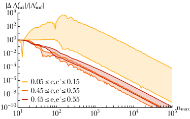
Figure 12: Illustration of the relative errors in the bare coupling coefficient, ${\Lambda_{\mathbf{n}\mathbf{n}^{\prime}}^{\ell}(\mathbf{J},\mathbf{J}^{\prime})}$, using the basis method as in Eq. (82) vs. the multipole expression from Eq. (86), as a function of the total number of basis elements, $n_{\max}$. Following Eq. (49), the angular integrals were performed using ${K\!=\!10^{5}}$ steps, with ${\ell\!=\!1}$, ${\mathbf{n}\!=\!(2,1)}$ and ${\mathbf{n}^{\prime}\!=\!(3,1)}$, and a potential basis satisfying ${R_{\mathrm{b}}\!=\!10\,b_{\mathrm{c}}}$. We considered $10^{4}$ pairs of orbits with ${x\!=\!1.0}$ and ${x^{\prime}\!=\!1.2}$, with the associated eccentricities, $e$ and $e^{\prime}$, taken uniformly within some finite range. Coloured regions correspond to the ${16\%}$ and ${84\%}$ levels among the pairs of orbits. We note in particular that the basis method converges significantly more slowly for quasi-circular orbits (in yellow).

In that figure, we note in particular that for quasi-circular orbits, the bare coupling coefficients are affected by (very) significant errors associated with the finite truncation of the number of basis elements.

Let us now detail how one may mitigate these errors when computing the dressed coupling coefficients as defined in Eq. (78). We assume that ${\mathbf{N}_{\ell}(\omega)\!\to\!\mathbf{I}}$, for ${p,q\!\geq\!n_{\mathrm{cut}}}$, and compute the full susceptibility matrix ${\mathbf{N}_{\ell}(\omega)}$ only for ${1\!\leq\!p,q\!\leq\!n_{\mathrm{cut}}}$. Then for the remaining $p,q>n_{\mathrm{cut}}$, we use the bare coefficients, so that Eq. (78) becomes

$$\Lambda_{\mathbf{n}\mathbf{n}^{\prime}}^{\ell}(\mathbf{J},\mathbf{J}^{\prime},\omega)=y_{\ell}^{n_{2}}\,y_{\ell}^{n^{\prime}_{2}}\bigg{\{}{} \sum_{\mathclap{p,q=1}}^{n_{\mathrm{cut}}}W_{\ell p}^{\mathbf{n}}(\mathbf{J})\,N_{pq}^{\ell}(\omega)\,W^{\mathbf{n}^{\prime}}_{\ell q}(\mathbf{J}^{\prime})$$

$$+{} \sum_{\mathclap{p=n_{\mathrm{cut}}+1}}^{+\infty}W_{\ell p}^{\mathbf{n}}(\mathbf{J})\,W_{\ell p}^{\mathbf{n}^{\prime}}(\mathbf{J}^{\prime})\bigg{\}},$$ (88)

Using Eq. (82), this can be rewritten as

$$\Lambda_{\mathbf{n}\mathbf{n}^{\prime}}^{\ell}(\mathbf{J},\mathbf{J}^{\prime},\omega)=y_{\ell}^{n_{2}}\,y_{\ell}^{n^{\prime}_{2}}\bigg{\{}{} \sum_{\mathclap{p,q=1}}^{n_{\mathrm{cut}}}W_{\ell p}^{\mathbf{n}}(\mathbf{J})\,\big{[}N_{pq}^{\ell}(\omega)\!-\!\delta_{pq}\big{]}W_{\ell q}^{\mathbf{n}^{\prime}}(\mathbf{J}^{\prime})$$

$$+{} W_{\ell}^{\mathbf{n}\mathbf{n}^{\prime}}(\mathbf{J},\mathbf{J}^{\prime})\bigg{\}},$$ (89)

where, importantly, the last term is obtained through the multipole expression from Eq. (87), that does not require any basis elements. We used such an expression to compute the BL fluxes in Fig. 4.

F.3 Convergence of the resonance truncation

The RR flux from Eq. (9) involves a sum over two resonance vectors ${\mathbf{n},\mathbf{n}^{\prime}}$. As highlighted in Eq. (78), for a given harmonic number $\ell$, the two resonance numbers $n_{2}$ and ${n^{\prime}_{2}}$ satisfy ${|n_{2}|,|n^{\prime}_{2}|\!\leq\!\ell}$. Yet, there are no such constraints for other resonance numbers $n_{1}$ and $n^{\prime}_{1}$. In practice, we mitigate this issue by limiting ourselves to ${|n_{1}|,|n^{\prime}_{1}|\!\leq\!n_{1}^{\max}}$, where $n_{1}^{\max}$ is a given threshold.

In Fig. 13, we explore the effect of this truncation on the value of the bare RR diffusion flux $\mathbf{F}_{\mathrm{RR}}^{\ell}$. First we computed the flux $\mathbf{F}_{\mathrm{RR}}^{\ell}$ at the same orbital location as in Fig. 2 and using ${n_{1}^{\max}\!=\!256}$. Different coloured lines in Fig. 13 show the relative error w.r.t. this measurement that is induced by degrading the calculation of $\mathbf{F}_{\mathrm{RR}}^{\ell}$ to smaller values of $n_{1}^{\max}$.

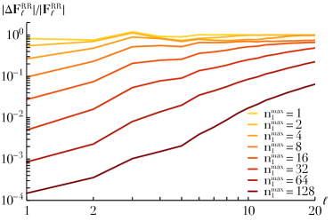
Figure 13: Illustration of the relative error in $\mathbf{F}_{\mathrm{RR}}^{\ell}$, computed at the same orbital location as in Fig. 2, as a function of the maximum resonance number, $n_{1}^{\max}$, and the considered harmonics $\ell$. Here, we used ${K\!=\!512}$ nodes to compute the orbit-average and ${K_{\mathrm{res}}\!=\!512}$ points to construct the resonance line. Relative errors are computed by comparison to a calculation with ${n_{1}^{\max}\!=\!256}$. The larger $\ell$ is, the more high-order resonances contribute.

As expected, the larger $\ell$ is, the larger $n_{1}^{\max}$ must be for an accurate calculation of the diffusion flux. In practice, it appears that picking ${n_{1}^{\max}\gtrsim 8\!+\!4\ell}$ allows for a computation of the flux with a relative error of the order of ${10\%}$, highlighting the role played by high-order resonances in driving the RR relaxation. More important conceptually is the fact that, at fixed $\ell$, the infinite sum over $n_{1}$ and $n^{\prime}_{1}$ in Eq. (13) converges, in sharp constrast with the logarithmic divergence w.r.t. the harmonic number $\ell$ highlighted in Fig. 2.

F.4 Multipole expansion

We now detail how the bare coupling coefficients, ${W_{\ell}^{\mathbf{n}\mathbf{n}^{\prime}}(\mathbf{J},\mathbf{J}^{\prime})}$, from Eq. (87) may be efficiently computed using a multipole approach. First, in order not to have to invert the implicit relation ${\theta_{1}\!=\!\theta_{1}(r)}$ (see Eq. (32)), and to avoid boundary divergences at the edge of the integration domain where the radial velocity vanishes, we rely on the same effective anomaly, ${r\!=\!r(u)}$, as in Eq. (48). Equation (87) then becomes

$$W_{\ell}^{\mathbf{n}\mathbf{n}^{\prime}}(\mathbf{J},\mathbf{J}^{\prime})=\frac{4}{\pi^{2}}\!\!\int_{-1}^{1}\!\!\frac{\mathrm{d}u}{2}\frac{\mathrm{d}u^{\prime}}{2}\,g(r)\,g^{\prime}(r^{\prime})\,U_{\ell}(r,r^{\prime}),$$ (90)

where we introduced the function

$$g(r)=\frac{\mathrm{d}\theta_{1}}{\mathrm{d}u}\,\cos\big{(}n_{1}\theta_{1}+n_{2}(\theta_{2}-\varphi)\big{)},$$ (91)

and similarly for ${g^{\prime}(r^{\prime})}$.

To perform the two integrals from Eq. (90), we now sample uniformly each interval using $K$ nodes. Specifically, for ${1\!\leq\!k\!\leq\!K}$, we sample the anomaly $u$ with

$$u_{k}=-1+\Delta u\,\big{(}k-\tfrac{1}{2}\big{)}\quad\text{ with }\quad\Delta u=\frac{2}{K}.$$ (92)

Following this discretisation, Eq. (90) becomes

$$W_{\ell}^{\mathbf{n}\mathbf{n}^{\prime}}\!\!=\!\frac{16G}{\pi(2\ell+1)}\frac{1}{K^{2}}\sum_{i,j}g_{i}\,g^{\prime}_{j}\,\frac{\mathrm{Min}[r_{i},r^{\prime}_{j}]^{\ell}}{\mathrm{Max}[r_{i},r^{\prime}_{j}]^{\ell+1}},$$ (93)

where we used the shortened notation ${g_{i}\!=\!g(r_{i})}$.

Let us now use the particular structure of Eq. (93) to accelerate its evaluation. To proceed forward, we order the set of radii ${\{r_{i},r^{\prime}_{j}\}}$ by increasing order. We emphasise that this can be made in ${\mathcal{O}(K)}$ steps, as the two sets ${\{r_{i}\}}$ and ${\{r^{\prime}_{j}\}}$ are already ordered, so that it only remains to merge the two lists. Following this ordering, we construct the array $w_{j}$ which, for ${1\!\leq\!j\!\leq\!K}$, is defined as

$$w_{j}=\mathrm{Card}\bigg{\{}i\in\big{\{}1,...,K\big{\}}\,\bigg{|}\,r_{i}\leq r^{\prime}_{j}\bigg{\}},$$ (94)

with the boundary terms ${w_{0}\!=\!0}$ and ${w_{K+1}\!=\!K}$. We can now rewrite the double sum from Eq. (93) as

$$W_{\ell}^{\mathbf{n}\mathbf{n}^{\prime}}\!\!=\!\frac{16G}{\pi(2\ell+1)}\frac{1}{K^{2}}\sum_{j=1}^{K}g^{\prime}_{j}\big{[}P_{j}+Q_{j}\big{]},$$ (95)

where we introduced

$$P_{j}=\sum_{i=1}^{w_{j}}g_{i}\frac{r_{i}^{\ell}}{r_{j}^{\prime\ell+1}};\quad Q_{j}=\sum_{\mathclap{i=w_{j}+1}}^{K}g_{i}\frac{r_{j}^{\prime\ell}}{r_{i}^{\ell+1}}.$$ (96)

Here, it is essential to note that both ${\{P_{j}\}_{1\leq j\leq K}}$ and ${\{Q_{j}\}_{1\leq j\leq K}}$ series can be computed with a complexity scaling linearly with $K$. To highlight this point, we define for ${1\!\leq\!j\!\leq\!K}$, the partial sums

$$\delta P_{j}=\sum_{\mathclap{i=w_{j-1}+1}}^{w_{j}}g_{i}\,\frac{r_{i}^{\ell}}{r_{j}^{\prime\ell+1}};\quad\delta Q_{j}=\sum_{\mathclap{i=w_{j}+1}}^{w_{j+1}}g_{i}\,\frac{r_{j}^{\prime\ell}}{r_{i}^{\ell+1}},$$ (97)

which satisfy the recurrence relations

$$P_{1}{} =\delta P_{1};\quad P_{j+1}=\bigg{[}\frac{r^{\prime}_{j}}{r^{\prime}_{j+1}}\bigg{]}^{\ell+1}\,P_{j}+\delta P_{j+1},$$

$$Q_{K}{} =\delta Q_{K};\quad Q_{j-1}=\bigg{[}\frac{r^{\prime}_{j-1}}{r^{\prime}_{j}}\bigg{]}^{\ell}\,Q_{j}+\delta Q_{j-1}.$$ (98)

Owing to these explicit recurrence relations, we are in a position to compute the bare coupling coefficients, ${W_{\ell}^{\mathbf{n}\mathbf{n}^{\prime}}(\mathbf{J},\mathbf{J}^{\prime})}$, with a complexity in ${\mathcal{O}(K)}$.

As a closing remark, let us detail a bit more the preparation of Eq. (93). In that equation, one must compute ${\theta_{1}[u_{k}]}$ and ${(\theta_{2}\!-\!\varphi)[u_{k}]}$. This is done using the same method as in Eq. (49), i.e. using a RK4 integration of each expression. In practice, the initial value of the various integrals are obtained through a first ‘warm-up’ starting from ${u\!=\!-1}$ with one RK4 step of length ${\Delta u/2}$.

In practice, for the maps presented in Fig. 5, we considered the resonances up to ${|n_{1}|,|n^{\prime}_{1}|\!\leq\!40}$ contained within the domain ${0\!\leq\!x\!\leq\!x_{\mathrm{max}}\!=\!10}$. The orbit-average was performed with ${K\!=\!200}$ points, and the resonance lines constructed with ${K_{\mathrm{res}}\!=\!200}$ points.

F.5 Softened bare coupling coefficients

It is also possible to obtain the bare coupling coefficients associated with a softened pairwise interaction of the form

$$U(\mathbf{r},\mathbf{r}^{\prime},\varepsilon)=-\frac{G}{\sqrt{|\mathbf{r}-\mathbf{r}^{\prime}|^{2}+\varepsilon^{2}}},$$ (99)

with $\varepsilon$ the considered softening length. Following §B of Weinberg (1986) (see also Wachlin & Carpintero (2006)), in the case of a softened interaction, Eq. (85) becomes

$$U_{\ell}(r,r^{\prime},\varepsilon)=\frac{4\pi G}{2\ell+1}\frac{r_{\beta}^{\ell}}{r_{\alpha}^{\ell+1}},$$ (100)

where we introduced the notations

$$r_{\alpha}{} =\!\bigg{[}\!\tfrac{1}{2}\bigg{(}\!r^{2}\!+\!r^{\prime 2}\!+\!\varepsilon^{2}\!+\!\sqrt{\!\big{(}(r\!+\!r^{\prime})^{2}\!+\!\varepsilon^{2}\big{)}\big{(}(r\!-\!r^{\prime})^{2}\!+\!\varepsilon^{2}\big{)}}\bigg{)}\!\bigg{]}^{1/2},$$

$$r_{\beta}{} =\frac{r\,r^{\prime}}{r_{\alpha}}.$$ (101)

From Eq. (101), one can immediately recover the unsoftened limit presented in Eq. (85). Unfortunately, the expression from Eq. (100) is far from being (almost) separable, so that it cannot benefit from the fast evaluation permitted by the multipole approach from §F.4.

We finally note that, even for the softened interaction kernel from Eq. (100), one can perform the same asymptotic expansion as in Eq. (15), as already detailed in Eq. (B8) of Weinberg (1986). As such, let us assume that ${r\!=\!b_{\mathrm{c}}}$, ${r^{\prime}\!=\!b_{\mathrm{c}}(1\!-\!\alpha)}$, with ${\alpha\!>\!0}$. Assuming that ${\mathcal{O}(\alpha)\!\simeq\!\mathcal{O}(\varepsilon)}$, one can write the following expansions

$$r_{\alpha}{} \simeq b_{\mathrm{c}}+\mathcal{O}(\varepsilon),$$

$$\frac{r_{\beta}}{r_{\alpha}}{} \simeq 1-\sqrt{\alpha^{2}+(\varepsilon/b_{\mathrm{c}})^{2}}+\mathcal{O}(\varepsilon^{2}).$$ (102)

As a consequence, in the limit ${\alpha,\varepsilon\!\ll\!1}$ and ${\ell\!\geq\!1}$, one can expand Eq. (100) as

$$U_{\ell}(\alpha){} \propto\frac{1}{b_{\mathrm{c}}}\,\Big{(}1-\sqrt{\alpha^{2}+(\varepsilon/b_{\mathrm{c}})^{2}}\Big{)}^{\ell}$$

$$\simeq\frac{1}{b_{\mathrm{c}}}\,\mathrm{e}^{-\ell\sqrt{\alpha^{2}+(\varepsilon/b_{\mathrm{c}})^{2}}}.$$ (103)

This is the direct equivalent of Eq. (16) in the case of a softened interaction. In particular, we note that for interparticle separations, $\alpha$, smaller than the softening length, $\varepsilon$, the pairwise coupling tends to a constant value. This prevents the system from sustaining any relaxation on scales smaller than the softening scale.

Appendix G Isochrone potential

In this section, we follow Hénon (1959), and recall some of the key analytical expressions of the isochrone potential used throughout the paper. It is defined as

$$\psi(r)=-\frac{GM}{b_{\mathrm{c}}+\sqrt{b_{\mathrm{c}}^{2}+r^{2}}},$$ (104)

with $M$ the system’s total active mass, and $b_{\mathrm{c}}$ its lengthscale. In practice, for all the numerical applications, we pick units so that ${G\!=\!M\!=\!b_{\mathrm{c}}\!=\!1}$. The isochrone Hamiltonian can be explicitly written as a function of the action coordinates. It reads

$$H(\mathbf{J})=-\frac{(GM)^{2}}{2{[J_{r}+\tfrac{1}{2}(L+\sqrt{L^{2}+4GMb_{\mathrm{c}}})]}^{2}}.$$ (105)

Fortunately, that same expression also provides us with an explicit inversion of the expression of the radial action, so that

$$J_{r}=\frac{GM}{\sqrt{-2E}}-\frac{1}{2}\bigg{(}L+\sqrt{L^{2}+4GMb_{\mathrm{c}}}\bigg{)}.$$ (106)

The radial frequency is given by

$$\Omega_{1}=\omega(a,e)\,\Omega_{0},$$ (107)

with the frequency scale ${\Omega_{0}\!=\!\sqrt{GM/b_{\mathrm{c}}^{3}}}$. In Eq. (107), we introduced the dimensionless function

$$\omega(a,e)=\bigg{(}\frac{E}{E_{\mathrm{min}}}\bigg{)}^{3/2}\!\!=\bigg{(}\frac{2}{s_{\mathrm{p}}\!+\!s_{\mathrm{a}}}\bigg{)}^{3/2},$$ (108)

where we introduced ${s_{\mathrm{p}}\!=\!\sqrt{1\!+\!x_{\mathrm{p}}^{2}}}$ (similarly for $s_{\mathrm{a}}$) with the dimensionless pericentre, ${x_{\mathrm{p}}\!=\!r_{\mathrm{p}}/b_{\mathrm{c}}}$, as well as the minimum energy ${E_{\mathrm{min}}\!=\!-GM/(2b_{\mathrm{c}})}$. The azimuthal frequency is given by

$$\Omega_{2}=\omega(a,e)\,\eta(a,e)\,\Omega_{0},$$ (109)

where we introduced the frequency ratio ${\eta\!=\!\Omega_{2}/\Omega_{1}}$. In the isochrone case, it follows the explicit form

$$\eta(a,e){} =\frac{1}{2}\bigg{(}1+\frac{L}{\sqrt{L^{2}+4GMb_{\mathrm{c}}}}\bigg{)}$$ (110)

$$=\frac{1}{2}\bigg{(}1\!+\!\frac{x_{\mathrm{p}}x_{\mathrm{a}}}{\big{(}1+s_{\mathrm{p}}\big{)}\big{(}1+s_{\mathrm{a}}\big{)}}\bigg{)}.$$

We note that along circular (resp. radial) orbits, i.e. for ${e\!\to\!0}$ (resp. ${e\!\to\!1}$), the isochrone frequencies take the simple forms

$$\begin{cases}\displaystyle\omega_{\mathrm{circ}}(x)=\bigg{(}\!\frac{1}{\sqrt{1\!+\!x^{2}}}\!\bigg{)}^{3/2},\\[8.61108pt] \displaystyle\eta_{\mathrm{circ}}(x)=\frac{\sqrt{1\!+\!x^{2}}}{1\!+\!\sqrt{1\!+\!x^{2}}},\end{cases}\!\!\!\begin{cases}\displaystyle\omega_{\mathrm{rad}}(x)=\bigg{(}\!\frac{2}{1\!+\!\sqrt{1\!+\!4x^{2}}}\!\bigg{)}^{3/2}\!\!,\\[8.61108pt] \displaystyle\eta_{\mathrm{rad}}(x)=\frac{1}{2}.\end{cases}$$ (111)

In the specific case of the isochrone potential, one can also get numerically well-posed expressions for ${E\!=\!E(r_{\mathrm{p}},r_{\mathrm{a}})}$ and ${L\!=\!L(r_{\mathrm{p}},r_{\mathrm{a}})}$ from Eq. (34). They read

$$E=\frac{E_{0}}{s_{\mathrm{p}}\!+\!s_{\mathrm{a}}};\quad L=\sqrt{2}\,L_{0}\,\frac{x_{\mathrm{p}}x_{\mathrm{a}}}{\sqrt{(1\!+\!s_{\mathrm{p}})(1\!+\!s_{\mathrm{a}})(s_{\mathrm{p}}\!+\!s_{\mathrm{a}})}},$$ (112)

with the energy scale ${E_{0}\!=\!-GM/b_{\mathrm{c}}}$, and the action scale ${L_{0}\!=\!\sqrt{GMb_{\mathrm{c}}}}$. These explicit expressions finally allow us to obtain exact expressions for the Jacobian ${\mathrm{d}\theta_{1}/\mathrm{d}u}$ appearing in Eq. (49)

$$\frac{\mathrm{d}\theta_{1}}{\mathrm{d}u}=\frac{3}{\sqrt{2}}\frac{\Omega_{1}}{\Omega_{0}}\,\frac{x_{r}}{\sqrt{4\!-\!u^{2}}}\,\frac{\sqrt{(s_{r}\!+\!s_{\mathrm{p}})(s_{r}\!+\!s_{\mathrm{a}})(s_{\mathrm{p}}\!+\!s_{\mathrm{a}})}}{\sqrt{(x_{r}\!+\!x_{\mathrm{p}})(x_{r}\!+\!x_{\mathrm{a}})}},$$ (113)

where we introduced ${x_{r}\!=\!r/b}$, and ${s_{r}\!=\!\sqrt{1\!+\!x_{r}^{2}}}$. Importantly, we note that this expression is numerically well-behaved for any ${-1\!\leq\!u\!\leq\!1}$.

Following Eq. (4.54) of Binney & Tremaine (2008), the isotropic DF of the isochrone potential reads

$$F_{\mathrm{tot}}(E)={} \,\frac{M}{(GMb_{\mathrm{c}})^{3/2}}\,\frac{1}{128\sqrt{2}\,\pi^{3}}\,\frac{\sqrt{\mathcal{E}}}{(1\!-\!\mathcal{E})^{4}}$$

$$\times{} \,\bigg{[}27\!-\!66\mathcal{E}\!+\!320\mathcal{E}^{2}\!-\!240\mathcal{E}^{3}+64\mathcal{E}^{4}$$

$$+\frac{3\sin^{-1}(\sqrt{\mathcal{E}})}{\sqrt{\mathcal{E}(1\!-\!\mathcal{E})}}(-9\!+\!28\mathcal{E}\!+\!16\mathcal{E}^{2})\bigg{]}.$$ (114)

where we introduced the rescaled energy ${\mathcal{E}\!=\!E/E_{0}}$. Owing to Eq. (114), one can compute all the gradients ${\partial F/\partial\mathbf{J}}$ that appear both in the response matrix from Eq. (44) and in the RR diffusion flux from Eq. (10).

In §B.3, we validate our implementation of the response matrix by recovering the radial orbit instability in a radially anisotropic isochrone cluster following Saha (1991). In that case, we consider an anisotropic DF defined as

$$F_{\mathrm{tot}}(Q)=\frac{M}{(GMb_{\mathrm{c}})^{3/2}}\frac{1}{128\sqrt{2}\,\pi^{3}}\frac{\sqrt{Q}}{(1\!-\!Q)^{4}}$$ (115)

$$\times{} \bigg{\{}27\!+\!77\gamma\!-\!(66\!+\!286\gamma)Q\!+\!(320\!+\!136\gamma)Q^{2}$$

$$\!-\!(240\!+\!32\gamma)Q^{3}\!+\!64Q^{4}$$

$$+{} \frac{3\sin^{-1}\big{(}\sqrt{Q}\big{)}}{\sqrt{Q(1\!-\!Q)}}\big{[}(-9\!+\!17\gamma)\!+\!(28\!-\!44\gamma)Q\!+\!(16\!-\!8\gamma)Q^{2}\big{]}\bigg{\}},$$

where we introduced

$$Q=\frac{1}{E_{0}}\bigg{(}E+\frac{L^{2}}{2R_{\mathrm{a}}^{2}}\bigg{)};\quad\gamma=\bigg{(}\frac{b_{\mathrm{c}}}{R_{\mathrm{a}}}\bigg{)}^{2}.$$ (116)

Here $R_{\mathrm{a}}$ is the so-called anisotropy radius. Stars orbiting at radii much smaller than $R_{\mathrm{a}}$ tend to have isotropically distributed velocities while stars at radii much larger than $R_{\mathrm{a}}$ are nearly all on highly radial orbits. In the limit ${R_{\mathrm{a}}\!\to\!+\infty}$, one has ${Q\!\to\!\mathcal{E}}$ and ${\gamma\!\to\!0}$, so that Eq. (115) reduces to Eq. (114).

In order to compute the resonant flux from Eq. (10), one has to compute a resonance condition of the form ${\delta_{\mathrm{D}}(\mathbf{n}\!\cdot\!\mathbf{\Omega}(\mathbf{J})\!-\!\mathbf{n}^{\prime}\!\cdot\!\mathbf{\Omega}(\mathbf{J}^{\prime}))}$. As already defined in Eq. (79), this amounts to finding all the resonant locations ${(x^{\prime},e^{\prime})}$ such that the resonance condition ${\mathbf{n}^{\prime}\!\cdot\!\mathbf{\Omega}(x^{\prime},e^{\prime})\!=\!\mathbf{n}\!\cdot\!\mathbf{\Omega}(\mathbf{J})}$ is satisfied. In conjunction with the computation of the response matrix, this is one of the most cumbersome tasks in the estimation of the RR diffusion flux. Fortunately, such a search can be eased in the case of the isochrone potential, owing to the explicit expressions of the associated orbital frequencies obtained in Eqs. (108) and (110). Let us now briefly detail our scheme to construct the system’s resonance lines.

Following Eq. (10), a resonance is characterised by a resonance vector ${\mathbf{n}^{\prime}\!=\!(n^{\prime}_{1},n^{\prime}_{2})}$. Following Eqs. (107) and (109), the associated resonance condition reads

$$\omega_{\mathrm{res}}(x^{\prime},e^{\prime})=\varpi,$$ (117)

where we introduced the resonance frequency ${\omega_{\mathrm{res}}\!=\!\omega(n^{\prime}_{1}\!+\!n^{\prime}_{2}\eta)}$, as well as the rescaled frequency ${\varpi\!=\!\mathbf{n}\!\cdot\!\mathbf{\Omega}(\mathbf{J})/\Omega_{0}}$.

First, we compute the quantity

$$\nu\equiv n^{\prime}_{1}+\tfrac{1}{2}n^{\prime}_{2}.$$ (118)

Owing to the simple expression of $\eta_{\mathrm{rad}}$ from Eq. (111), we have the inequality ${|\omega_{\mathrm{res}}(x,e\!=\!1)|\leq|\nu|}$, and the function ${x^{\prime}\!\mapsto\!\omega(x^{\prime},e\!=\!1)}$ is a monotonic function. As a consequence, dealing appropriately with the case ${\nu\!=\!0}$, we may conclude that the resonance line goes up to the radial orbit if one has

$$0\leq\frac{\varpi}{\nu}\leq 1.$$ (119)

If this constraint is satisfied, the resonance line reaches radial orbits for ${x^{\prime}\!=\!x^{\prime}_{\mathrm{rad}}}$ so that ${\omega_{\mathrm{res}}(x^{\prime}_{\mathrm{rad}},e^{\prime})\!=\!\varpi}$ with the explicit expression

$$x^{\prime}_{\mathrm{rad}}=\frac{\sqrt{1-(\varpi/\nu)^{2/3}}}{(\varpi/\nu)^{2/3}}.$$ (120)

Having determined whether or not the resonance line reaches the radial orbits, we must now consider how it reaches the circular orbit. Along circular orbits, the resonance frequency takes the form

$$\omega_{\mathrm{res}}(x^{\prime},e^{\prime}\!=\!0)=\frac{1}{q^{3/2}}\bigg{[}n^{\prime}_{1}+n^{\prime}_{2}\,\frac{q}{1+q}\bigg{]}\equiv h(q),$$ (121)

where we introduced ${q\!=\!\sqrt{1+x^{2}}}$. We note therefore that the boundary terms are given by ${\omega_{\mathrm{res}}(x^{\prime}\!=\!0,e^{\prime}\!=\!0)\!=\!\nu}$ and ${\omega_{\mathrm{res}}(x^{\prime}\!=\!+\infty,e^{\prime}\!=\!0)\!=\!0}$. Since these are the same bounds as in Eq. (119), we conclude that any resonance line that reaches the radial orbits necessarily reaches the circular orbits.

For some resonance vector, ${(n^{\prime}_{1},n^{\prime}_{2})}$, the function ${q\!\mapsto\!h(q)}$ might not be monotonic. Yet, we have the systematic bound ${|h(q)|\!\leq\!(|n^{\prime}_{1}\!+\!n^{\prime}_{2}|)/q^{3/2}}$, so that introducing

$$q_{\mathrm{b}}=\bigg{(}\frac{2(|n^{\prime}_{1}|\!+\!|n^{\prime}_{2}|)}{|\varpi|}\bigg{)}^{2/3},$$ (122)

one gets that ${q\!\leq\!q_{\mathrm{b}}}$ implies ${|h(q)|\!\leq\!|\varpi|/2}$. In the case where Eq. (119) is satisfied, such a bound provides us with an explicit interval within which to perform a bisection search in order to obtain the location at which the resonance line intersects the circular orbits, $x^{\prime}_{\mathrm{circ}}$. Once ${(x^{\prime}_{\mathrm{circ}},x^{\prime}_{\mathrm{rad}})}$ have been determined, we sample uniformly the range ${0\!\leq\!e^{\prime}\!\leq\!1}$ with $K_{\mathrm{res}}$ points, and we use bisection searches to identify precisely the resonance locations. In practice, we also ensure that the resonant search is constrained to the domain ${0\!\leq\!x^{\prime}\!\leq\!x_{\mathrm{max}}}$.

Even if the condition from Eq. (119) is not met, the system can still support a resonance line that would not reach radial orbits, but would rather connect two circular orbits. To find such lines, we follow Eq. (121) and write

$$\frac{\mathrm{d}h}{\mathrm{d}q}=\frac{P(q)}{2q^{5/2}(1+q)^{2}},$$ (123)

where we introduced the second-order polynomial

$$P(q)=-3(n^{\prime}_{1}\!+\!n^{\prime}_{2})q^{2}-(6n^{\prime}_{1}+n^{\prime}_{2})q-3n^{\prime}_{1}.$$ (124)

We note that if ${n^{\prime}_{2}\!=\!-n^{\prime}_{1}}$, ${P(q)}$ becomes linear in $q$. In the range ${1\!\leq\!q\!\leq\!+\infty}$ this function is of constant sign, i.e. the function ${h(q)}$ is monotonic. As a consequence, for such resonances, we may use the exact same criteria as in Eq. (119), and all the resonance lines connect the circular orbits to the radial ones.

Let us then assume ${n^{\prime}_{2}\!\neq\!n^{\prime}_{1}}$. The polynomial ${P(q)}$ from Eq. (124) is then a true second-order polynomial, and its discriminant reads

$$\Delta=n^{\prime}_{2}(n^{\prime}_{2}-24n^{\prime}_{1}).$$ (125)

If ${\Delta\!\leq\!0}$, ${P(q)}$ does not change sign. As a consequence, ${h(q)}$ is monotonic. The criteria from Eq. (119) applies again, and all the resonance lines connect the circular orbits to the radial ones.

If ${\Delta\!>\!0}$, ${P(q)}$ has two roots, i.e. it changes of sign. It only remains to determine whether or not this change of sign occurs within the domain ${1\!\leq\!q\!<\!+\infty}$. The two roots of ${P(q)}$ are given by

$$q_{\pm}=\frac{-(6n^{\prime}_{1}+n^{\prime}_{2})\pm\sqrt{\Delta}}{6(n^{\prime}_{1}+n^{\prime}_{2})},$$ (126)

which are subsequently ordered as

$$q_{\mathrm{min}}=\mathrm{Min}[q_{-},q_{+}];\quad q_{\mathrm{max}}=\mathrm{Max}[q_{-},q_{+}].$$ (127)

It is only if ${1\!<\!q_{\mathrm{max}}}$ that the system can support resonance line joining two circular orbits. In that case, we use a bisection search to identify these two radii $x^{\prime}_{\mathrm{min}}$ and $x^{\prime}_{\mathrm{max}}$ where the resonance condition is met. We then sample uniformly the range ${x^{\prime}_{\mathrm{min}}\!\leq\!x^{\prime}\!\leq\!x^{\prime}_{\mathrm{max}}}$ with $K_{\mathrm{res}}$ points and we use bisection searches to identify precisely the resonance locations. In practice, we also enforce the additional constraint that the resonance line is limited to the domain ${0\!\leq\!x^{\prime}\!\leq\!x_{\mathrm{max}}}$.

To conclude this Appendix, we briefly illustrate in Fig. 14 an example of resonance lines, where one can note, as previously discussed, the presence of two types of resonance lines depending on whether or not they reach radial orbits.

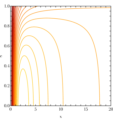
Figure 14: Illustration of the level lines of the resonance frequency ${\omega_{\mathrm{res}}\!=\!\mathbf{n}\!\cdot\!\mathbf{\Omega}(x,e)}$ for an isochrone cluster, considering the resonance vector ${\mathbf{n}\!=\!(4,-7)}$. In particular, one can note that there exist two types of resonance lines, depending on whether or not they reach radial orbits (${e\!=\!1}$).

Appendix H Numerical simulations

In this Appendix, we briefly detail the properties of our numerical simulations.

In order to ease the description of each of these setups, for this Appendix, units are displayed in Hénon units ($\mathrm{HU}$) (Hénon, 1971). For the isochrone potential from Eq. (104), the virial theorem gives the system’s velocity dispersion as (see, e.g., Eq. (B36) in Hamilton et al., 2018)

$$\sigma^{2}=\frac{GM}{b_{\mathrm{c}}}\bigg{(}\frac{\pi}{4}-\frac{2}{3}\bigg{)}.$$ (128)

As a result, the lengthscale of the Henon units is given by

$$r_{\mathrm{H}}=\frac{6}{3\pi-8}\,b_{\mathrm{c}}\simeq 4.21\,b_{\mathrm{c}}.$$ (129)

In order to sample the cluster’s initial condition, we adapted the publicly available code PlummerPlus to the case of an isotropic isochrone cluster. All simulations were performed with a total of ${N\!=\!10^{5}}$ particles of equal mass.

H.1 Collisional simulations

In order to simulate the dynamics of the globular cluster as driven by the (unsoftened) Newtonian interaction, we used the direct code NBODY6++GPU (Wang et al., 2015), with the control parameters

$$\texttt{NNBOPT}\!=\!400;\;\texttt{ETAI}\!=\!0.02;\;\texttt{ETAR}\!=\!0.01;$$

$$\texttt{RS0}\!=\!0.10;\;\texttt{DTADJ}\!=\!2.0;\;\texttt{QE}\!=\!2\!\times\!10^{-4};$$

$$\texttt{DTMIN}\!=\!10^{-5};\;\texttt{RMIN}\!=\!2\!\times\!10^{-4};\;\texttt{ETAU}\!=\!0.1;$$ (130)

$$\texttt{ECLOSE}\!=\!1.0;\;\texttt{GMIN}\!=\!10^{-6};\;\texttt{GMAX}\!=\!0.01;\;\texttt{SMAX}\!=\!0.125.$$

Each individual realisation was run on a node with a single GPU and a 40-core CPU. Integrating one realisation up to ${t_{\mathrm{max}}\!=\!10^{3}\,\mathrm{HU}}$ required about $26$h of computation. We performed a total of ${N_{\mathrm{real}}\!=\!10^{2}}$ different realisations.

H.2 Collisionless simulations

In order to simulate the dynamics of the globular cluster as driven by the softened Plummer interaction kernel from Eq. (99), we used the collisionless code gyrfalcON (Dehnen, 2000). Simulations were performed using the Plummer softening kernel $P_{0}$, which matches exactly with Eq. (99). Integration parameters were chosen so that the integration time step is ${\Delta t\!=\!2^{-8}\,\mathrm{HU}}$, while the minimum tolerance parameter was fixed to ${\theta\!=\!0.6}$.

To fix the softening length, we followed the same approach as in Theuns (1996) (see Eq. (14) therein). In the very core of the cluster, the typical interparticle distance is given by

$$d=\big{[}\mu/\rho(0)\big{]}^{1/3}.$$ (131)

For the isochrone potential (see Eq. (2.49) of Binney & Tremaine, 2008), this simply becomes

$$d{} =\big{[}16\pi/(3N)\big{]}^{1/3}\,b_{\mathrm{c}}$$

$$\simeq 0.013\,\mathrm{HU}\;\;\;\;\;\;\;\text{for}\;\;N=10^{5}.$$ (132)

It is then appropriate to consider a softening length comparable with this scale. In practice, for the fiducial runs, we used ${\varepsilon\!=\!d/2}$. Each individual realisation was run on a single CPU-core. Integrating one realisation up to ${t_{\mathrm{max}}\!=\!10^{3}\,\mathrm{HU}}$ required about $17$h of computation. We performed a total of ${N_{\mathrm{real}}\!=\!168}$ different realisations with ${\varepsilon\!=\!0.0065\,\mathrm{HU}}$.

H.3 Measuring the diffusion rate

As recently investigated in Heggie et al. (2020) (see also references therein), the density centre of the cluster undergoes a correlated random walk throughout its relaxation. It is therefore of prime importance to correctly centre the coordinate system before attempting any measurement of the particles’ actions.

In the collisional runs, to estimate the position of the density centre, we followed the algorithm from Casertano & Hut (1985) using the ${j\!=\!6}$ nearest neighbours to estimate the local densities. In the collisionless runs, we used the same algorithm with ${j\!=\!32}$.

Once the origin of the coordinate system has been determined, we checked that the cluster’s mean potential had scarcely changed from the initial mean isochrone potential. We could then use the particles’ position and velocities ${(\mathbf{r},\mathbf{v})}$ to estimate their energy and angular momentum ${(E,L)}$, and finally the associated actions ${(J_{r},L)}$, following Eq. (106). Having determined the particle’s actions at the initial time ${t\!=\!0}$, and at the late time ${t\!=\!10^{3}\,\mathrm{HU}}$, we binned particles into ${20\!\times\!20}$ bins within the domain ${0\!\leq\!J_{r}\!\leq\!0.4\,\mathrm{HU}}$ and ${0\!\leq\!L\!\leq\!0.7\,\mathrm{HU}}$. This allowed us to compute the variation in the number of particles within each action bin through a simple difference between both times. Once averaged over available realisations, this led to a direct estimation of ${\partial F(\mathbf{J})/\partial t}$, as presented in Figs. 6 and 8.

References

- Bar-Or & Alexander (2016) Bar-Or B., Alexander T., 2016, ApJ, 820, 129
- Bar-Or & Fouvry (2018) Bar-Or B., Fouvry J.-B., 2018, ApJ, 860, L23
- Binney & Lacey (1988) Binney J., Lacey C., 1988, MNRAS, 230, 597
- Binney & Tremaine (2008) Binney J., Tremaine S., 2008, Galactic Dynamics: Second Edition. Princeton Univ. Press
- Breen et al. (2017) Breen P. G., Varri A. L., Heggie D. C., 2017, MNRAS, 471, 2778
- Casertano & Hut (1985) Casertano S., Hut P., 1985, ApJ, 298, 80
- Chandrasekhar (1943) Chandrasekhar S., 1943, ApJ, 97, 255
- Chavanis (2012) Chavanis P.-H., 2012, Physica A, 391, 3680
- Chavanis (2013a) Chavanis P.-H., 2013a, Eur. Phys. J. Plus, 128, 126
- Chavanis (2013b) Chavanis P.-H., 2013b, A&A, 556, A93
- Clutton-Brock (1973) Clutton-Brock M., 1973, Ap&SS, 23, 55
- Dehnen (2000) Dehnen W., 2000, ApJ, 536, L39
- Drukier et al. (1999) Drukier G., Cohn H., Lugger P., Yong H., 1999, ApJ, 518, 233
- Edmonds (1996) Edmonds A., 1996, Angular Momentum in Quantum Mechanics. Princeton Univ. Press
- Fouvry et al. (2015) Fouvry J.-B., Pichon C., Magorrian J., Chavanis P.-H., 2015, A&A, 584, A129
- Fouvry et al. (2019) Fouvry J.-B., Bar-Or B., Chavanis P.-H., 2019, ApJ, 883, 161
- Giersz & Heggie (1994) Giersz M., Heggie D. C., 1994, MNRAS, 268, 257
- Gilbert (1968) Gilbert I. H., 1968, ApJ, 152, 1043
- Hamilton (2021) Hamilton C., 2021, MNRAS, 501, 3371
- Hamilton & Heinemann (2020) Hamilton C., Heinemann T., 2020, arXiv, 2011.14812
- Hamilton et al. (2018) Hamilton C., Fouvry J.-B., Binney J., Pichon C., 2018, MNRAS, 481, 2041
- Heggie & Hut (2003) Heggie D., Hut P., 2003, The Gravitational Million-Body Problem
- Heggie et al. (2020) Heggie D. C., Breen P. G., Varri A. L., 2020, MNRAS, 492, 6019
- Hénon (1959) Hénon M., 1959, Annales d’Astrophysique, 22, 126
- Hénon (1960) Hénon M., 1960, Annales d’Astrophysique, 23, 668
- Hénon (1971) Hénon M., 1971, Ap&SS, 14, 151
- Heyvaerts (2010) Heyvaerts J., 2010, MNRAS, 407, 355
- Kalnajs (1976) Kalnajs A. J., 1976, ApJ, 205, 745
- Kim et al. (2008) Kim E., Yoon I., Lee H. M., Spurzem R., 2008, MNRAS, 383, 2
- Lau & Binney (2019) Lau J. Y., Binney J., 2019, MNRAS, 490, 478
- Meiron & Kocsis (2019) Meiron Y., Kocsis B., 2019, ApJ, 878, 138
- Nelson & Tremaine (1999) Nelson R. W., Tremaine S., 1999, MNRAS, 306, 1
- Pichon (1994) Pichon C., 1994, Dynamics of self-gravitating disks. Cambridge Univ.
- Press et al. (2007) Press W., et al., 2007, Numerical Recipes 3rd Edition. Cambridge Univ. Press
- Rauch & Tremaine (1996) Rauch K. P., Tremaine S., 1996, New Astron., 1, 149
- Rogister & Oberman (1968) Rogister A., Oberman C., 1968, J. Plasma Phys., 2, 33
- Rozier et al. (2019) Rozier S., Fouvry J.-B., Breen P. G., Varri A. L., Pichon C., Heggie D. C., 2019, MNRAS, 487, 711
- Saha (1991) Saha P., 1991, MNRAS, 248, 494
- Sellwood (2015) Sellwood J., 2015, MNRAS, 453, 2919
- Takahashi (1995) Takahashi K., 1995, PASJ, 47, 561
- Theuns (1996) Theuns T., 1996, MNRAS, 279, 827
- Tremaine & Weinberg (1984) Tremaine S., Weinberg M. D., 1984, MNRAS, 209, 729
- Vasiliev (2015) Vasiliev E., 2015, MNRAS, 446, 3150
- Wachlin & Carpintero (2006) Wachlin F. C., Carpintero D. D., 2006, Rev. Mex. Astron. Astrofis., 42, 251
- Wang et al. (2015) Wang L., Spurzem R., Aarseth S., Nitadori K., Berczik P., Kouwenhoven M. B. N., Naab T., 2015, MNRAS, 450, 4070
- Weinberg (1986) Weinberg M. D., 1986, ApJ, 300, 93
- Weinberg (1989) Weinberg M. D., 1989, MNRAS, 239, 549
- Weinberg (1994) Weinberg M. D., 1994, ApJ, 421, 481
- e Silva et al. (2017) e Silva L. B., de Siqueira Pedra W., Sodré L., Perico E. L., Lima M., 2017, ApJ, 846, 125