Lossless compression with state space models using bits back coding

Abstract

We generalize the ‘bits back with ANS’ method to time-series models with a latent Markov structure. This family of models includes hidden Markov models (HMMs), linear Gaussian state space models (LGSSMs) and many more. We provide experimental evidence that our method is effective for small scale models, and discuss its applicability to larger scale settings such as video compression.

1 Introduction

Recent work by Townsend et al. (2019) shows the existence of a practical method, called ‘bits back with ANS’ (BB-ANS), for doing lossless compression with a latent variable model, at rates close to the negative variational free energy of the model (this quantity bounds the model’s marginal log-likelihood and is often referred to as the ‘evidence lower bound’, or ELBO). BB-ANS depends on a last-in-first-out (LIFO) source coding algorithm called Asymmetric Numeral Systems (ANS; Duda, 2009), and also uses an idea called bits back coding (Wallace, 1990; Hinton & van Camp, 1993). Townsend et al. (2019) show that BB-ANS can be used to compress sequences of symbols which are modeled as statistically independent. The compression rate achieved for the first symbol compressed is equal to the ELBO plus the entropy of the approximate posterior, which is a significant overhead, but compression rates for subsequent symbols are very close to the ELBO. For long enough sequences, the effect of the first symbol overhead on the overall compression rate is negligible.

Townsend et al. (2019) demonstrated BB-ANS on MNIST images using a small VAE. Subsequent work has extended BB-ANS to hierarchical latent variable models and larger, color images (Townsend et al., 2020; Kingma et al., 2019) and demonstrated how to use ideas from the Monte Carlo literature to achieve a tighter bound than the ELBO (Ruan et al., 2021). In this work we present a generalization of BB-ANS to sequences which are not modeled as independent, by ‘interleaving’ bits-back steps with the time-steps in a model, exploiting latent Markov structure in a similar way to the Bit-Swap method of Kingma et al. (2019). We call the method ‘Interleaving for economical Compression with Latent Sequence Models’ (IconoCLaSM).

IconoCLaSM is applicable to the general class of ‘state space models’ (SSMs; defined in section 2.2), but does require access to specific conditional distributions under an approximate posterior (section 3). We demonstrate the method on a hidden Markov model (HMM; Baum & Petrie, 1966), showing that, as with vanilla BB-ANS, for long enough sequences the compression rate is very close to the model ELBO. We believe that this result is significant, because the same method is likely to be extensible to audio and video compression with deep latent variable models.

2 Background

2.1 Asymmetric Numeral Systems

Asymmetric Numeral Systems (ANS) is a family of algorithms for losslessly compressing sequences (Duda, 2009). ANS defines a last-in-first-out (LIFO) compressed message data structure and the inverse pair of functions ‘push’ and ‘pop’, for adding and removing data from the message.

To encode a sequence $x_{1},\ldots,x_{T}$, with distribution $P$, ANS encoding starts with a very short base message $m_{\mathrm{init}}$, and then encodes the elements one-at-a-time, starting with $x_{T}$ and working backwards:

$$m_{T} =\mathrm{push}_{P(x_{T}\,|\,x_{1},\ldots,x_{T-1})}(m_{\mathrm{init}},x_{T})$$ (1)

$$m_{T-1} =\mathrm{push}_{P(x_{T-1}\,|\,x_{1},\ldots,x_{T-2})}(m_{T},x_{T-1})$$ (2)

$$\kern 5.5pt\vdots$$

$$m_{1} =\mathrm{push}_{P(x_{1})}(m_{2},x_{1}).$$ (3)

The compressed message $m_{1}$ can then be communicated and data decoded forwards using the inverse sequence of pop operations. Each push depends on the cumulative distribution function (CDF) and its inverse for the conditional distribution $P(x_{t}\,|\,x_{1},\ldots,x_{t-1})$.

It can be shown that the length, in bits, of the message after each push operation is bounded above

$$l(m_{t})<h(x_{t},\ldots,x_{T}\,|\,x_{1},\ldots,x_{t-1})+t\epsilon+C,$$ (4)

where $h(x):=1/\log_{2}P(x)$ is the ‘information content’, and $C$ and $\epsilon$ are implementation-dependent constants. Since $C$ does not depend on $t$, the per-symbol compression rate tends towards $h(x_{t}\,|\,x_{1},\ldots,x_{t-1})+\epsilon$ as $T$ increases. In a typical ANS implementation, $C=64$ and $\epsilon\approx 2.2\times 10^{-5}$; Townsend (2020) provides more detail. Thus, for long enough sequences, ANS encodes close to the information content, and it is not possible to do better on average for data sampled from $P$ (Shannon, 1948).

After pushing some data, it is then possible to pop using a different distribution. Doing so produces a sample from the distribution used for popping, and shortens the message length by the information content of that sample. Using such intermediate decoding steps within an encoding process is the key idea behind bits back coding, which is significantly more flexible than basic ANS.

Hereafter we elide $m$ and use the shorthand notation of Townsend et al. (2020): $x\rightarrow P(x)$ for pushing the symbol $x$ according to the distribution $P$, and $x\leftarrow P(x)$ for the inverse pop operation.

2.2 Latent variable models and state space models

For the purposes of this work, we define a latent variable model to be a model with a mass function which can be expressed as a sum or integral over a ‘latent’ variable $z$:

$$P(x\,|\,\theta)=\int P(x\,|\,z,\theta)\,P(z\,|\,\theta)\;dz,$$ (5)

where $\theta$ denotes the parameters of the model. The marginal distribution $P(x\,|\,\theta)$ needn’t be tractable: our model is defined by the ‘prior’ $P(z\,|\,\theta)$ and ‘likelihood’ $P(x\,|\,z,\theta)$. The parameters $\theta$ can be learned by optimizing the ‘evidence lower bound’ (ELBO):

$$L(x;\theta,\phi)=\mathbb{E}_{Q(z\,|\,x,\phi)}\log\frac{P(x,z\,|\,\theta)}{Q(z\,|\,x,\phi)},$$ (6)

where $Q$ is a variational distribution, referred to as the ‘approximate posterior’, and $\phi$ are the ‘variational parameters’. The ELBO is usually optimized jointly with respect to $\theta$ and $\phi$ using stochastic gradient ascent (Kingma & Welling, 2014; Rezende et al., 2014). Coding with BB-ANS (section 2.3), requires access to conditional CDFs and inverse CDFs under the prior, likelihood and approximate posterior, as described in section 2.1. From now on we assume access to a trained model (i.e., with $\theta$ and $\phi$ fixed).

State space models (SSMs) are latent variable models where an observed sequence $x_{1},\ldots,x_{T}$ is modeled using a latent sequence $z_{1},\ldots,z_{T}$ and the joint mass function admits the factorization

$$P(x_{1},\ldots,x_{T},z_{1},\ldots,z_{T})=P(z_{1})\prod_{t=2}^{T}P(z_{t}\,|\,z_{t-1})\prod_{t=1}^{T}P(x_{t}\,|\,z_{t}).$$ (7)

In general, both the observations and the latents may be either continuous or discrete, but for lossless compression we require discrete observations. SSMs have been applied to speech modeling, computational neuroscience and many other areas (Kalman, 1960; Rabiner, 1989; Paninski et al., 2010), and using deep, nonlinear SSMs for video modeling is an active area of research (Johnson et al., 2016; Saxena et al., 2021).

2.3 Bits back with ANS

To compress a symbol $x$ using ANS with a latent variable model, a naive thing to do would be to choose $z$ and send it along with the data:

$$x \rightarrow P(x\,|\,z)$$ (8)

$$z \rightarrow P(z).$$ (9)

These operations increase message length by $\log 1/P(x,z)$, so the optimal choice of $z$ is one which minimizes that quantity. That increase is longer than the ideal length $\log 1/P(x)$, because of a redundancy: $z$ has effectively been sent twice: once the receiver has decoded $x$, they can compute $z$ by running the same minimization routine that the sender used.

The idea of bits-back coding (Wallace, 1990; Hinton & van Camp, 1993) is to recover information communicated in the choice of $z$, in a way that cancels out the redundancy. BB-ANS (Townsend et al., 2019) is a practical realization of this idea that codes at an average rate equal to the negative ELBO. The BB-ANS sender decodes $z$ according to $Q$. That is, they sample a plausible latent value $z$ from the approximate posterior $Q$, using the information in the message to make the random choice.

The BB-ANS encoding and decoding processes are as follows:

BB-ANS encoding process

⬇

1$z\leftarrow Q(z\,|\,x)$

2$x\rightarrow P(x\,|\,z)$

3$z\rightarrow P(z)$

BB-ANS decoding process

⬇

1$z\leftarrow P(z)$

2$x\leftarrow P(x\,|\,z)$

3$z\rightarrow Q(z\,|\,x)$

When the first symbol $x$ is encoded, the message $m$ is empty, so the posterior sample $z$ is generated at random, rather than decoded. This leads to an ‘initial bits’ overhead of $\log 1/Q(z\,|\,x)$ for the first symbol. Once a sufficient buffer has been built up in $m$, $z$ can be decoded and the compression rate of subsequent steps will be close to the negative ELBO. If $Q$ is equal to the exact posterior $P(z\,|\,x)$, then the ELBO bound is tight and BB-ANS is close to optimal (Townsend et al., 2019).

3 Coding with state space models using IconoCLaSM

In order to use an SSM for lossless compression, we could directly apply BB-ANS. However, the first step of encoding in BB-ANS is to decode an entire latent, and in the case of an SSM that means sampling the sequence $z_{1},\ldots,z_{T}$; leading to an initial bits overhead which scales with $T$, making this an impractical method. We could break the sequence into independent chunks, but this would also harm the compression rate. The central contribution of this work is a method for ‘interleaving’ bits back steps with the SSM timesteps, allowing optimal compression with $O(1)$ initial bits overhead. The encoding and decoding processes are shown below.

IconoCLaSM requires the following factorization of the approximate posterior:

$$Q(z_{1},\ldots,z_{T}\,|\,x_{1},\ldots,x_{T})=Q(z_{T}\,|\,x_{1},\ldots,x_{T})\prod_{t=1}^{T-1}Q(z_{t}\,|\,x_{1},\ldots,x_{t},z_{t+1}),$$ (10)

and that the factors on the right hand side can be coded with ANS (i.e., their CDFs and inverse CDFs are available). In HMMs and linear Gaussian SSMs those factors can be computed exactly using message passing. In deep latent variable models they may be computed using an RNN, as in Saxena et al. (2021), or by message passing, as in Johnson et al. (2016).

IconoCLaSM encoding process

⬇

1$z_{T}\leftarrow Q(z_{T}\,|\,x_{1},\ldots,x_{T})$

2for $t$ in $T,\ldots,2$:

3 $x_{t}\rightarrow P(x_{t}\,|\,z_{t})$

4 $z_{t-1}\leftarrow Q(z_{t-1}\,|\,x_{1},\ldots,x_{t-1},z_{t})$

5 $z_{t}\rightarrow P(z_{t}\,|\,z_{t-1})$

6$x_{1}\rightarrow P(x_{1}\,|\,z_{1})$

7$z_{1}\rightarrow P(z_{1})$

IconoCLaSM decoding process

⬇

1$z_{1}\leftarrow P(z_{1})$

2$x_{1}\leftarrow P(x_{1}\,|\,z_{1})$

3for $t$ in $2,\ldots,T$:

4 $z_{t}\leftarrow P(z_{t}\,|\,z_{t-1})$

5 $z_{t-1}\rightarrow Q(z_{t-1}\,|\,x_{1},\ldots,x_{t-1},z_{t})$

6 $x_{t}\leftarrow P(x_{t}\,|\,z_{t})$

7$z_{T}\rightarrow Q(z_{T}\,|\,x_{1},\ldots,x_{T})$

4 Experiments

We conducted proof of concept experiments to demonstrate IconoCLaSM on a small hidden Markov model; that is, an SSM with discrete latents and observations. Since, in an HMM, the conditionals $P(x_{t}\,|\,x_{1},\ldots,x_{t-1})$ can be tractably computed using message passing, it is possible to use vanilla ANS with this model. As a result, IconoCLaSM is not the most efficient way to code with an HMM. However, an HMM is a reasonable first demonstration of IconoCLaSM, since the HMM has the correct generative structure, the required posterior conditionals are available, and we can easily compare to the exact information content.

  

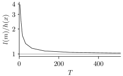
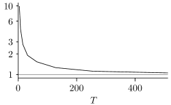
Figure 1: Plots showing that the ratio of the actual compressed message length, $l(m)$, to the information content $h(x)$, tends to $1$ as the sequence length $T$ increases. Left hand plot is compressing data sampled from the model; right hand plot is compressing English text with a model trained using the EM algorithm.

Figure 1 shows the convergence of the compression rate to the optimum, $h(x)$, as the sequence length $T$ increases, for two different setups. For the first experiment, shown in the left hand plot, we compressed an exact sample from an HMM with randomly generated parameters. Then, to demonstrate that IconoCLaSM doesn’t depend on the model being perfectly fit to the data, for the second plot we compressed a section of War and Peace, using an HMM trained on an earlier section of the same text. The effect of the initial bits overhead is significant for short messages, but diminishes gracefully as sequence length increases.

The HMMs used for both experiments had 64 hidden states. The HMM for the first experiment had 64 observation states and all parameters sampled from a Dirichlet distribution with concentration parameters $\alpha_{i}\!=\!1$. The HMM for the second experiment had 101 observation states (corresponding to the characters that appeared in the text) and parameters trained using the EM algorithm for 100 iterations. Code to reproduce these experiments is available at github.com/j-towns/ssm-code.

5 Discussion

We have demonstrated the existence of a simple, practical scheme for doing lossless compression with state space models, assuming the availability of certain conditionals under a (possibly approximate) posterior. It was demonstrated by Kingma et al. (2019) and Townsend et al. (2020) that the basic BB-ANS method can be scaled up to large, color images. We speculate that it may be possible to scale up IconoCLaSM in a similar way, and use it for lossless compression of video, where deep latent variable models have been shown to be effective (Saxena et al., 2021; Johnson et al., 2016). Two particularly interesting open questions are

1. Can IconoCLaSM be generalized to hierarchical models, and if so what constraints are there on the hierarchical model and posterior?

2. Can IconoCLaSM be combined with Monte Carlo methods such as sequential Monte Carlo in order to improve on the ELBO, in the style of Ruan et al. (2021)?

We leave investigation of these questions to future work.

References

- Baum & Petrie (1966) Leonard E. Baum and Ted Petrie. Statistical Inference for Probabilistic Functions of Finite State Markov Chains. The Annals of Mathematical Statistics, 37(6):1554–1563, 1966.
- Duda (2009) Jarek Duda. Asymmetric numeral systems, 2009. http://arxiv.org/abs/0902.0271.
- Hinton & van Camp (1993) Geoffrey E. Hinton and Drew van Camp. Keeping Neural Networks Simple by Minimizing the Description Length of the Weights. In Proceedings of the Sixth Annual Conference on Computational Learning Theory, COLT ’93, pp. 5–13, 1993.
- Johnson et al. (2016) Matthew J. Johnson, David K. Duvenaud, Alex Wiltschko, Ryan P. Adams, and Sandeep R. Datta. Composing graphical models with neural networks for structured representations and fast inference. In Advances in Neural Information Processing Systems 29, pp. 2946–2954. 2016.
- Kalman (1960) Rudolf E. Kalman. A New Approach to Linear Filtering and Prediction Problems. Journal of Basic Engineering, 82(1):35–45, 1960.
- Kingma & Welling (2014) Diederik P. Kingma and Max Welling. Auto-Encoding Variational Bayes. In International Conference on Learning Representations (ICLR), 2014.
- Kingma et al. (2019) Friso H. Kingma, Pieter Abbeel, and Jonathan Ho. Bit-Swap: Recursive Bits-Back Coding for Lossless Compression with Hierarchical Latent Variables. In International Conference on Machine Learning, 2019.
- Paninski et al. (2010) Liam Paninski, Yashar Ahmadian, Daniel Gil Ferreira, Shinsuke Koyama, Kamiar Rahnama Rad, Michael Vidne, Joshua Vogelstein, and Wei Wu. A new look at state-space models for neural data. Journal of Computational Neuroscience, 29(1):107–126, 2010.
- Rabiner (1989) L. R. Rabiner. A tutorial on hidden Markov models and selected applications in speech recognition. Proceedings of the IEEE, 77(2):257–286, 1989.
- Rezende et al. (2014) Danilo Jimenez Rezende, Shakir Mohamed, and Daan Wierstra. Stochastic Backpropagation and Approximate Inference in Deep Generative Models. In International Conference on Machine Learning, pp. 1278–1286, 2014. http://proceedings.mlr.press/v32/rezende14.html.
- Ruan et al. (2021) Yangjun Ruan, Karen Ullrich, Daniel Severo, James Townsend, Ashish Khisti, Arnaud Doucet, Alireza Makhzani, and Chris J. Maddison. Improving Lossless Compression Rates via Monte Carlo Bits-Back Coding, 2021. http://arxiv.org/abs/2102.11086.
- Saxena et al. (2021) Vaibhav Saxena, Jimmy Ba, and Danijar Hafner. Clockwork Variational Autoencoders, 2021. http://arxiv.org/abs/2102.09532.
- Shannon (1948) Claude. E. Shannon. A mathematical theory of communication. The Bell System Technical Journal, 27(3):379–423, 1948.
- Townsend (2020) James Townsend. A tutorial on the range variant of asymmetric numeral systems, 2020. http://arxiv.org/abs/2001.09186.
- Townsend et al. (2019) James Townsend, Thomas Bird, and David Barber. Practical lossless compression with latent variables using bits back coding. In International Conference on Learning Representations (ICLR), 2019. https://openreview.net/forum?id=ryE98iR5tm.
- Townsend et al. (2020) James Townsend, Thomas Bird, Julius Kunze, and David Barber. HiLLoC: Lossless image compression with hierarchical latent variable models. In International Conference on Learning Representations (ICLR), 2020. https://openreview.net/forum?id=r1lZgyBYwS.
- Wallace (1990) Chris S. Wallace. Classification by minimum-message-length inference. In Advances in Computing and Information, pp. 72–81, 1990.