Search and Matching for Adoption from Foster Care

Search and Matching for Adoption from Foster Care

N. Olberg, L. Dierks, S. Seuken, V. Slaugh, and U. Ünver

Nils Olberg Department of Informatics, University of Zurich, Switzerland, olberg@ifi.uzh.ch Ludwig Dierks Department of Informatics, Kyushu University, Japan, dierks@inf.kyushu-u.ac.jp Sven Seuken Department of Informatics, University of Zurich, Switzerland, seuken@ifi.uzh.ch Vincent W. Slaugh SC Johnson College of Business, Cornell University, USA, vslaugh@cornell.edu M. Utku Ünver Department of Economics, Boston College, USA, unver@bc.edu

More than 100,000 children in the foster care system are currently waiting for an adoptive placement in the United States, where adoptions from foster care occur through a semi-decentralized search and matching process with the help of local agencies. Traditionally, most agencies have employed a family-driven search process, where prospective families respond to announcements made by the caseworker responsible for a child. However, recently some agencies switched to a caseworker-driven search process, where the caseworker conducts a targeted search of suitable families for the child. We introduce a novel search-and-matching model to capture essential aspects of adoption and compare these two search processes through a game-theoretical analysis. We show that the search equilibria induced by (novel) threshold strategies form a lattice structure under either approach. Our main theoretical result establishes that the equilibrium outcomes in family-driven search can never Pareto dominate the outcomes in caseworker-driven search, but there are instances where each caseworker-driven search outcome Pareto dominates all family-driven search outcomes. We also find that when families are sufficiently impatient, caseworker-driven search is better for all children. We illustrate numerically that for a wide range of parameters, most agents are better off under caseworker-driven search.

child adoption, foster care, search and matching, market design, game theory

1 Introduction

Foster care systems worldwide serve children suffering from abuse, neglect, or other crises by temporarily removing them from their families until a permanent solution can be found. For example, the United States foster care system serves around 700,000 children annually, with approximately 440,000 children in foster care at any given point in time. While the goal for most of these children is to reunite them with their parents or close relatives, roughly 120,000 children are waiting for adoptive placements (Children’s Bureau 2020). Finding a permanent family for these children has become a public policy priority due to high levels of incarceration, homelessness, unemployment, and teen pregnancy observed in the population of children “aging out” of long-term foster care (Barth 1990, Triseliotis 2002, Courtney et al. 2010).

A caseworker, typically a social worker employed by county agencies or non-profit organizations, represents the child in the process of finding suitable adoptive parents (simply families from now on). This process has a search and a matching aspect: Identifying a family that is willing to adopt the child and capable of meeting the child’s needs from this large pool of candidates can be like searching for a needle in a haystack. A priori, caseworkers do not know whether a family would be a suitable match. Caseworkers must carefully review written home studies (i.e., documents providing background information about families) and perform interviews. This can be a time consuming and emotional stressful process for everyone involved. Furthermore, a match between a child and a family only forms if both the child (represented by the caseworker) and the family agree to the match. If all involved parties agree to a match, the child is placed with the family usually for a test period of several months. Once the test period has been completed successfully, the adoption is finalized. In this paper, we study and model the search and matching process (adoption matching from now on) for children waiting for adoptive placement and compare two prominent search methods for finding suitable families for these children.

There are different paradigms for the practice of search and matching. In the predominant approach, caseworkers announce children via email to a set of registered families, each of whom has the opportunity to express interest in a child. The caseworker receives these inquiries and works to identify the family that best fits the needs of the child. We label this approach family-driven search, as families take a lead role in the search process. However, some child welfare agencies have recently sought to improve outcomes by switching to caseworker-driven search, in which caseworkers search using a database tool and target specific prospective parents. One motivation for this change is that caseworkers are usually better at identifying suitable matches than families. We provide a more detailed description of the two approaches in Appendix 9.

Even though caseworker-driven search might have its advantages, it is unclear whether it leads to overall desirable outcomes. One of the reasons is that changing the approach also affects how agents are going to strategically behave in the system. Taking these strategic effects into account is essential in order to determine whether a caseworker-driven search approach ultimately improves the overall process. In this paper, we therefore ask the following research question: Does caseworker-driven search lead to more desirable outcomes than family-driven search? In order to answer this question, we introduce a new search-and-matching model (Section 3), which captures the following key aspects: First, both approaches to adoption matching are inherently dynamic. Children and families (simply agents from now on) may enter and leave the system at any time, and there is no central matchmaking. Second, we allow for uncertainty regarding whether a child-family pair would actually be compatible. Third, our model captures the heterogeneous preferences of agents.

We perform a game-theoretic comparison of the two approaches within our model. In Section 4.2, we establish that equilibria are guaranteed to exist under both search technologies (i.e., family-driven search and caseworker-driven search). Furthermore, we find that equilibria form a lattice reminiscent of the structure of the set of stable matchings in standard two-sided matching markets. We then present our main theoretical result: Family-driven search equilibrium outcomes can never be Pareto improvements over caseworker-driven search equilibrium outcomes, but there are instances where each caseworker-driven search equilibrium outcome is a Pareto improvement over all family-driven search equilibrium outcomes (Section 5.1). This holds because caseworker-driven search (i) can reduce wasted search efforts and (ii) agents can worry less about accumulating search costs when they express interest in a child. However, because of multiplicity of equilibria and the lattice structure over these equilibria, all children can be strictly better off in either system. The same holds for families. Even when both family-driven search and caseworker-driven search only admit a unique equilibrium each, an agent can be better off in either setting (Section 5.2). This may be surprising, given that caseworker-driven search reduces wasteful search efforts on both sides of the market. We therefore explore the conditions under which caseworker-driven search usually leads to more agents being better off. In Section 6.1, we show that all children will be better off in caseworker-driven search if families are sufficiently impatient. Furthermore, increasing family supply in family-driven search can have a negative effect on children’s utilities, but not in caseworker-driven search (Section 6.2). We find numerically that caseworker-driven search leads to more desirable outcomes for a wide variety of model parameter choices (Section 7). We lastly discuss limitations of our model and the potential policy implications of our work (Section 8). With this work, we aim to inform current public policy questions as well as adoption agencies’ tactical matching efforts.

2 Related Work

Even though child adoption matching markets bear similarities to other two-sided matching markets such as centralized labor markets (Roth 1984, 1991) or ride sharing platforms (Ma et al. 2020), there are important differences that necessitate new models and analyses. Adoption matching is inherently dynamic, and there is no centralized clearinghouse that determines final matches. Matches are only ever proposed, and both sides of the market have to invest search efforts to identify a match candidate. Purely random decentralized matching models have been widely studied under search frictions and homogeneous preferences (Eeckhout 1999, Shimer and Smith 2000, 2001, Atakan 2006) and more rarely under heterogeneous preferences (Adachi 2003). More recent studies have combined directional search rather than random search as an important feature (Lauermann and Nöldeke 2014, Lauermann et al. 2020, Cheremukhin et al. 2020).

One matching market similar to adoption from foster care is online dating (Hitsch et al. 2010a, b, Lee and Niederle 2015, Rios et al. 2021, Kanoria and Saban 2021). However, online dating markets are completely decentralized despite their dynamic and recommendation-based features. Individuals in search of a romantic partner can, at any time, decide to browse a dating platform and reach out to other individuals that appeal to them. In contrast, the approaches we analyze in this paper follow a centralized protocol despite the dynamic decentralized search component: Caseworkers perform the search for a family on behalf of children, and they do so in approximately regular time intervals. Caseworkers therefore play an essential role throughout the process since they act as an intermediary to protect vulnerable children. Crucially, this introduces an asymmetry that we have not observed in any other previously studied matching market. As a consequence, we develop a new model that allows us to capture the features of the two different search technologies in one model.

Our paper contributes to the literature that studies child welfare systems from an economic perspective. Slaugh et al. (2016) investigated how the Pennsylvania Statewide Adoption & Permanency Network could utilize a match recommendation tool to improve their process of matching children to prospective parents. Their spreadsheet-based tool can be seen as a simplified version of the previously mentioned data-driven software system. Robinson-Cortés (2019) worked with a foster care data set to analyze placements of children in foster homes. His model predicts that allowing placements across administrative regions would be beneficial for children. MacDonald (2019) studied a dynamic matching problem where children and families can either form reversible matches (foster placements) or irreversible matches (adoptions). In her model, children are heterogeneous in the sense that there are children with disabilities and children without disabilities, while families are homogeneous. Baccara et al. (2014) estimate families’ preferences over children available for adoption from a data set documenting the operations of adoption agencies. A key difference of our paper from the earlier literature is that we allow for general heterogeneous preferences. While we focus specifically on analyzing adoption systems, our work is also relevant for search-and-matching theory in general. To the best of our knowledge, we are the first to formally analyze economic effects in the child welfare domain while taking heterogeneity of preferences into account.

The literature on dynamic matching relates to our work (Arnosti et al. 2021, Baccara et al. 2015, Immorlica et al. 2020, Jeloudar et al. 2021, Kasy and Teytelboym 2020). Again, the fact that none of these works allow for fully general preferences distinguishes them from our work. Different studies investigate how matching platforms should be designed so that desirable outcomes can be achieved (see, e.g., Lee and Niederle 2015, Fradkin 2017, Shi 2020). Most of these works perform field experiments, with the exception of Shi (2020), which is most related to our work since the author explores which side of the market should drive the search process depending on which side’s preferences can easily be expressed or satisfied. The setting, however, is quite different from our work since we allow agents on both sides of the market to arrive over time and let them face an optimal stopping problem as they can decide to remain unmatched until better future match opportunities arise.

Recently, there has been an increased interest from market design and related areas in historically underserved and disadvantaged communities (e.g., refugee resettlement Andersson et al. 2018, Bansak et al. 2018, Delacrétaz et al. 2020, improvement of teacher quality at disadvantaged schools Combe et al. 2022). We hope that the child welfare system will similarly receive more attention in the future.

3 Preliminaries

In this section, we first introduce the notation that is used in both family-driven search (FS) and caseworker-driven search (CS). We then describe the processes of the two different search technologies and derive characterizations of agents’ utilities.

3.1 Model

In our model, agents (children and families) have observable characteristics. Agents with the same characteristics are said to be of the same type. We treat sibling sets as single children in our model. Furthermore, we see the caseworker as a direct representative of the child, i.e., we think of a child-caseworker pair as one child agent. We let $C=\{c_{1},\ldots,c_{n}\}$ and $F=\{f_{1},\ldots,f_{m}\}$ denote the set of all $n$ child types and the set of all $m$ family types, respectively. Individual agents are indifferent between agents of the same type, i.e., their preferences are over agent types: A child of type $c$ has a value $v_{c}({f})\in\mathbb{R}$ for family type $f$, and a family of type $f$ has a value $v_{f}({c})\in\mathbb{R}$ for child type $c$. Preferences are assumed to be strict, i.e., $v_{c}({f})\neq v_{c}({f^{\prime}})$ if $f\neq f^{\prime}$ and $v_{f}({c})\neq v_{f}({c^{\prime}})$ if $c\neq c^{\prime}$. Agents’ valuations are summarized by a list of vectors $v=(v_{c_{1}},\ldots,v_{c_{n}},v_{f_{1}},\ldots,v_{f_{m}})$, and each agent has a value of 0 for remaining unmatched. Given valuations $v$, we let $\bar{v}$ denote the maximal value of all $v_{c}({f})$ and $v_{f}({c})$.

There are infinitely many discrete time steps. At any time step, there is at most one agent of each type present in the system. Thus, we can use $c\in C$ and $f\in F$ to refer to either individual agents and agent types without ambiguity. We refer to an agent (or agent type) from either set as $i\in A:=C\cup F$. From now on, we will simply say that agent $i\in A$ is active if they are present at the current time step.

At the beginning of each time step, all active agents are determined as follows: For each family type, one family of that type is active with with probability $\lambda\in(0,1]$. This is determined independently for each family type. We call parameter $\lambda$ the market thickness indicator, as it determines the expected number of active families at each time step: For small values of $\lambda$, there will be few active families in expectation. For large values of $\lambda$, it is quite likely that a family of each type will be active. Further, exactly one child (type) is selected uniformly at random to be active. This feature is motivated by search processes used by adoption agencies: A caseworker works on the case of one child at a time, which we assume she selects randomly.

There is uncertainty regarding whether a specific child $c$ and a specific family $f$ are compatible: With probability $p\in(0,1)$, $f$ is a suitable match for $c$ and unsuitable with probability $1-p$. Whether a match is suitable or not is determined independently at random for child-family pairs. We refer to $p$ as the match success probability. Parameter $p$ captures the following aspect of adoption markets: When a family shows interest in a child, the family’s decision is based on limited reported information, such as the sex, ethnicity, age of the child, and known disabilities. However, there are many other important characteristics of a child that determine whether the child is actually a good match for the family and whether there is mutual attraction. The same holds for a child (or his caseworker) showing interest in a family. Only if a family $f$ is a suitable match for child $c$ can a match between $c$ and $f$ be formed. If $c$ and $f$ form a match they both obtain a value of $v_{c}({f})$ and $v_{f}({c})$, respectively. Determining the suitability of a match is costly for both sides, as it is a time-consuming process. Children and families incur search costs $\kappa_{C}\in\mathbb{R}_{+}$ and $\kappa_{F}\in\mathbb{R}_{+}$, respectively, each time the suitability of a match including them is determined. All agents discount the future, however, they only discount time steps in which they are active. Children’s and families’ discount factors are $\delta_{C}\in[0,1)$ and $\delta_{F}\in[0,1)$, respectively.

We model adoption matching as a dynamic process that we assume to be stationary. An instance $(v,\delta_{C},\delta_{F},\kappa_{C},\kappa_{F},p,\lambda)$ together with a search technology (which we will introduce) induce a game. To reduce notation, we assume that instance $(v,\delta_{C},\delta_{F},\kappa_{C},\kappa_{F},p,\lambda)$ is fixed unless stated otherwise. Agents’ strategies in this game are captured as follows: Child $c$ is either interested in a family of type $f$ or not. Similarly, each family $f$ is either interested in a child of type $c$ or not. We assume that all agents of the same type play the same strategy, and agents don’t change their strategies in different time steps. Therefore, we can represent a strategy for a child $c$ as a vector $s_{c}\in\{0,1\}^{m}$, where $s_{c}(f)=1$ if $c$ is interested in matching with a family of type $f$. Similarly, a strategy for a family $f$ is given by a vector $s_{f}\in\{0,1\}^{n}$, where $s_{f}(c)$ indicates whether $f$ is interested in children of type $c$. A strategy profile is a tuple of vectors $s=(s_{c_{1}},\ldots,s_{c_{n}},s_{f_{1}},\ldots,s_{f_{m}})$, while we let $S$ denote the finite set of all possible strategy profiles. For $i\in A$ we let $s_{-i}$ denote the tuple of all agents’ strategies in $s$, except that agent $i$ is excluded. We say that $c$ and $f$ are mutually interested in each other under strategy profile $s$ if $s_{c}(f)=1$ and $s_{f}(c)=1$. The set $M(s)=\{(c,f)\in C\times F\mid s_{c}(f)=s_{f}(c)=1\}$ is called the matching correspondence of $s$. We use $M_{i}(s)$ to denote the set of agents that agent $i$ is mutually interested in under $s$.

In the remainder of this section, we describe the two different search technologies. We analyze the dynamic stochastic games induced by an instance and a search technology in a full information environment.

Family-driven Search (FS): At the beginning of each time step, after a child $c$ is randomly chosen to be active, each family that is active and interested in $c$ lets the caseworker of the child know of their interest. This corresponds to families responding to an email announcement made by a caseworker. The caseworker immediately discards any families without mutual interest in $c$, i.e., where $s_{c}(f)=0$ or $s_{f}(c)=0$. The caseworker then investigates all remaining families to determine whether they would actually be a suitable match. Recall that each investigated family is a suitable match for $c$ with probability $p$—which is determined independently for each family—and that each agent incurs cost for each investigation including them. After all families have been processed by the caseworker, $c$ either matches with the most-preferred choice from all those families that were identified as suitable matches or remains unmatched if no such family exists. We move on to the next time step.

Caseworker-driven Search (CS): After a child $c$ is randomly chosen to be active at the beginning of a time step, the child’s caseworker is presented with a list of active families ordered in decreasing order of $v_{c}({f})$. Families are then sequentially processed. The caseworker skips any family in which $c$ is not mutually interested. If there is mutual interest between $c$ and $f$, the suitability of a match between $c$ and $f$ is investigated. If the match turns out to be suitable, $c$’s search is over, $c$ and $f$ are matched and leave. We then move on to the next time step. Otherwise, the caseworker continues the search by selecting the next family in the list. If all families have been processed, the child remains unmatched and we move on to the next time step. Proposition 10.1 in Appendix 10.1 shows that $c$’s utility is maximized if the caseworker processes families in decreasing order of $v_{c}(f)$.

3.2 Utilities

We define agents’ utilities at a time step and characterize their flow utilities in both FS- and CS-induced stochastic games. Assume child $c$ is active at the current time step and that active families are yet to be determined. Let $f$ be an arbitrary family. For any $s\in S$, let $b_{cf}(s)=|\{f^{\prime}\in M_{c}(s)\mid v_{c}({f^{\prime}})>v_{c}({f})\}|$ denote the number of families in $M_{c}(s)$ that $c$ likes better than $f$. Further, let $\beta_{cf}(s)$ denote the probability that $c$ will not match with any other family that $c$ prefers over $f$ at the current time step. Noting that for any child $c$ the probability that a mutually interested family $f^{\prime}$ is active at the current time step and a suitable match is $\lambda p$, it follows immediately that $\beta_{cf}(s)=(1-\lambda p)^{b_{cf}(s)}$ for both FS and CS. In FS and CS, the expected immediate utility that active child $c$ will obtain at an arbitrary time step is then given by

$$\bar{u}^{FS}_{c}(s)=\lambda\sum_{f^{\prime}\in M_{c}(s)}\beta_{cf^{\prime}}(s)pv_{c}({f^{\prime}})-\kappa_{C}$$ (1)

and

$$\bar{u}^{CS}_{c}(s)=\lambda\sum_{f^{\prime}\in M_{c}(s)}\beta_{cf^{\prime}}(s)\left(pv_{c}({f^{\prime}})-\kappa_{C}\right),$$ (2)

respectively. Similarly, for a family $f$, we can express the expected immediate utilities at an arbitrary time step (conditional on $f$ being active) by

$$\bar{u}^{FS}_{f}(s)=\frac{1}{n}\sum_{c^{\prime}\in M_{f}(s)}\beta_{c^{\prime}f}(s)pv_{c^{\prime}}({f})-\kappa_{F}$$ (3)

for FS and

$$\bar{u}^{CS}_{f}(s)=\frac{1}{n}\sum_{c^{\prime}\in M_{f}(s)}\beta_{c^{\prime}f}(s)\left(pv_{c^{\prime}}({f})-\kappa_{F}\right)$$ (4)

for CS. From the previous equations the crucial difference between FS and CS in our model becomes immediately apparent: In FS, search costs are incurred with certainty if there is mutual interest between agents. In CS, however, search costs only incur if all previous match attempts at the time step have been unsuccessful.

We assume that each agent is risk neutral and maximizes their expected (overall) utility, which is the expected discounted value of their eventual match minus the total discounted search costs they incur. We use $(z)^{+}$ as shorthand-notation for $\max\{z,0\}$. $\mathbbm{1}\big{[}\cdot\big{]}$ is the indicator function, which has value $1$ if its argument is true and value $0$ otherwise. We denote the expected (overall) utility of agent $i$ under strategy profile $s$ by $u^{FS}_{i}(s)$ in FS and $u^{CS}_{i}(s)$ in CS. Whenever it is clear from context whether we are referring to FS or CS we will simply write $u_{i}(s)$. Proposition 3.1 characterizes children’s and families’ utilities in FS and CS via balance equations.

Proposition 3.1

Given strategy profile $s$, $c$’s utility in FS is the unique value $u^{FS}_{c}(s)$ that satisfies

$$u^{FS}_{c}(s)=\delta_{C}u^{FS}_{c}(s)+\lambda\sum_{f\in M_{c}(s)}\Big{(}\beta_{cf}(s)p\big{(}v_{c}({f})-\delta_{C}u^{FS}_{c}(s)\big{)}-\kappa_{C}\Big{)}.$$ (5)

Similarly, $f$’s utility in FS is the unique value $u^{FS}_{f}(s)$ that satisfies

$$u^{FS}_{f}(s)=\delta_{F}u^{FS}_{f}(s)+\frac{1}{n}\sum_{c\in M_{f}(s)}\Big{(}\beta_{cf}(s)p\big{(}v_{f}({c})-\delta_{F}u^{FS}_{f}(s)\big{)}-\kappa_{F}\Big{)}.$$ (6)

In CS, $c$’s utility in CS is the unique value $u^{CS}_{c}(s)$ that satisfies

$$u^{CS}_{c}(s)=\delta_{C}u^{CS}_{c}(s)+\lambda\sum_{f\in M_{c}(s)}\beta_{cf}(s)\Big{(}p\big{(}v_{c}({f})-\delta_{C}u^{CS}_{c}(s)\big{)}-\kappa_{C}\Big{)}.$$ (7)

Similarly, $f$’s utility in CS is the unique value $u^{CS}_{f}(s)$ that satisfies

$$u^{CS}_{f}(s)=\delta_{F}u^{CS}_{f}(s)+\frac{1}{n}\sum_{c\in M_{f}(s)}\beta_{cf}(s)\Big{(}p\big{(}v_{f}({c})-\delta_{F}u^{CS}_{f}(s)\big{)}-\kappa_{F}\Big{)}.$$ (8)

The proof of Proposition 3.1 can be found in Appendix 11.1. One difference between FS and CS is immediately visible from the above balance equations. In CS, search costs only incur if previous match attempts have been unsuccessful. In FS, however, costs incur with certainty if there is mutual interest and the family is active.

4 Equilibria

We use a tie-breaking assumption, which allows us to exclude degenerate equilibria later on. After stating this assumption, we introduce two classes of strategies—one for CS and one for FS—and show that these classes capture agents’ best responses. This will be helpful for obtaining results later on. We show that for both search technologies equilibria always exist and that equilibria form a lattice.

4.1 Threshold Strategies

For both search technologies, we make the following tie-breaking assumption: If agent $i$’s utility would (weakly) increase from mutual interest with agent $j$, then $i$ will be interested in $j$—even if $j$ is not interested in $i$. Similarly, if agent $i$’s utility would decrease from mutual interest with agent $j$, then $i$ will not be interested in $j$. This assumption allows us to exclude degenerate equilibria (e.g., no agent being interested in any other agent) later on without restricting agents in their endeavour to maximize their utility.

We now introduce threshold strategies for FS and CS. As we will see, our tie-breaking assumption implies that agents’ best responses belong to the class of threshold strategies. Note that a best response always exists, because $S$ is finite.

Definition 4.1

Child $c$ plays a CS threshold strategy (CS-TS) with threshold $y_{c}\in\mathbb{R}$ in $s$, if

$$s_{c}(f)=\mathbbm{1}\big{[}p(v_{c}({f})-\delta_{C}y_{c})\geq\kappa_{C}\big{]}\mbox{ for all }f\in F.$$ (9)

Family $f$ plays a CS-TS with threshold $y_{f}$ in $s$, if

$$s_{f}(c)=\mathbbm{1}\big{[}p(v_{f}({c})-\delta_{F}y_{f})\geq\kappa_{F}\big{]}\mbox{ for all }c\in C.$$ (10)

Child $c$ plays an FS threshold strategy (FS-TS) with threshold $y_{c}$ in $s$, if

$$s_{c}(f)=\mathbbm{1}\big{[}\beta_{cf}(s)p(v_{c}({f})-\delta_{C}y_{c})\geq\kappa_{C}\big{]}\mbox{ for all }f\in F.$$ (11)

Family $f$ plays an FS-TS with threshold $y_{f}$ in $s$, if

$$s_{f}(c)=\mathbbm{1}\big{[}\beta_{cf}(s)p(v_{f}({c})-\delta_{F}y_{f})\geq\kappa_{F}\big{]}\mbox{ for all }c\in C.$$ (12)

In a CS-TS or an FS-TS, threshold $y_{i}$ can be interpreted as $i$’s reservation utility. Let $u^{FS*}_{i}(s_{-i})$ and $u^{CS*}_{i}(s_{-i})$ denote $i$’s utility from a best response to $s_{-i}$ in FS and CS, respectively. As before, we simply write $u^{*}_{i}(s_{-i})$ if there is no ambiguity. Proposition 4.2 shows that agents’ best responses always have the form of a threshold strategy.

Proposition 4.2

Let $i\in A$ and $s_{-i}$ be an arbitrary strategy profile of all agents excluding $i$. In both FS and CS, a best response of $i$ to $s_{-i}$ corresponds to a threshold strategy with threshold $u^{*}_{i}(s_{-i})$.

The proof of Proposition 4.2 can be found in Appendix 11.2. To derive results later on, it will prove useful to switch between thresholds and strategies. We therefore provide the following definition.

Definition 4.3

In CS, a strategy profile induced by threshold profile $y\in\mathbb{R}^{n+m}$ is denoted by $s^{CS}(y)$ and satisfies for each $i\in A$, $s^{CS}_{i}(y)$ is a CS-TS with threshold $y_{i}$ in $s^{CS}(y)$. In FS, a strategy profile induced by threshold profile $y\in\mathbb{R}^{n+m}$ is denoted by $s^{FS}(y)$ and satisfies for each $i\in A$, $s^{FS}_{i}(y)$ is a FS-TS with threshold $y_{i}$ in $s^{FS}(y)$.

We again omit the superscript if this does not lead to ambiguity. It is trivial to obtain $s^{CS}(y)$ by inserting $y$ in the corresponding equations in Definition 4.1. Algorithm 1 from Appendix 12 can be used to compute $s^{FS}(y)$. From now on, we use $\beta^{FS}_{cf}(y)$ and $\beta^{CS}_{cf}(y)$ as shorthand-notation for $\beta_{cf}(s^{FS}(y))$ and $\beta_{cf}(s^{CS}(y))$, respectively. Whenever it is clear from the context, we simply write $\beta_{cf}(y)$.

4.2 Equilibrium Existence and Lattice Structure

In this section, we show that equilibria always exist under both search technologies. We use Nash equilibria as our equilibrium concept. We say that strategy profile $s$ is an equilibrium in FS (FSE) if $s$ is a Nash equilibrium in the game induced by FS. Analogously, strategy profile $s$ is an equilibrium in CS (CSE) if $s$ is a Nash equilibrium in the game induced by CS. We use $S^{FS}$ to denote the set of FSE, and let $Y^{FS}=\{(u_{i}(s))_{i\in A}\}_{s\in S^{FS}}$ be the corresponding set of equilibrium threshold profiles in FS. For CS, those sets are defined analogously. Before we can prove that these sets are never empty, we need to define a partial order $\leq_{C}$ on $Y=[0,\bar{v}]^{n+m}$. Note that if agents only play individually rational strategies their utility is always lower bounded by $0$ and upper bounded by $\bar{v}$.

Definition 4.4

Let $\leq_{C}$ be the partial order on $Y$, where for all $y,y^{\prime}\in Y$ it holds that $y\leq_{C}y^{\prime}$ if and only if $y_{c}\leq y^{\prime}_{c}$ for all $c\in C$ and $y_{f}\geq y^{\prime}_{f}$ for all $f\in F$.

Having defined partial order $\leq_{C}$, we can now prove that equilibria always exist in both settings. We state this result in Proposition 4.5.

Proposition 4.5

The set of FS and CS equilibrium threshold profiles $Y^{FS}$ and $Y^{CS}$ is non-empty and both $(Y^{FS},\leq_{C})$ and $(Y^{CS},\leq_{C})$ form complete lattices.

Proof 4.6

Proof. For FS, define a mapping $T^{FS}:Y\rightarrow Y$ as follows: $T^{FS}=(T^{FS}_{i})_{i\in A}$, where

$$T^{FS}_{c}(y)=\delta_{C}y_{c}+\lambda\sum_{f\in F}\mathbbm{1}[\beta_{cf}(y)p(v_{f}({c})-\delta_{F}y_{f})\geq\kappa_{F}]\Big{(}\beta_{cf}(y)p(v_{c}({f})-\delta_{C}y_{c})-\kappa_{C}\Big{)}^{+}$$ (13)

for all $c\in C$ and

$$T^{FS}_{f}(y)=\delta_{F}y_{f}+\frac{1}{n}\sum_{c\in C}\mathbbm{1}[\beta_{cf}(y)p(v_{c}({f})-\delta_{C}y_{c})\geq\kappa_{C}]\Big{(}\beta_{cf}(y)p(v_{f}({c})-\delta_{F}y_{f})-\kappa_{F}\Big{)}^{+}.$$ (14)

for all $f\in F$. Note that any fixed point of $T^{FS}$ (i.e., any $y$ with $T^{FS}(y)=y$) is an equilibrium threshold profile in FS. We now show that $T^{FS}$ is monotonically increasing according to $\leq_{C}$. Let $c\in C$, $y,y^{\prime}\in Y$, and $y\leq_{C}y^{\prime}$. We have

$$T^{FS}_{c}(y) =\delta_{C}y_{c}+\lambda\sum_{f\in F}\mathbbm{1}[\beta_{cf}(y)p(v_{f}({c})-\delta_{F}y_{f})\geq\kappa_{F}]\Big{(}\beta_{cf}(y)p(v_{c}({f})-\delta_{C}y_{c})-\kappa_{C}\Big{)}^{+}$$ (15)

$$\leq\delta_{C}y^{\prime}_{c}+\lambda\sum_{f\in F}\mathbbm{1}[\beta_{cf}(y^{\prime})p(v_{f}({c})-\delta_{F}y^{\prime}_{f})\geq\kappa_{F}]\Big{(}\beta_{cf}(y^{\prime})p(v_{c}({f})-\delta_{C}y^{\prime}_{c})-\kappa_{C}\Big{)}^{+}$$ (16)

$$=T^{FS}_{c}(y^{\prime}).$$ (17)

The inequality holds because of the following reason: Suppose a family $f$ is interested in $c$ under $s(y)$ but not under $s(y^{\prime})$. Since $f$ is weakly less selective in $s(y^{\prime})$, it must be the case that there exists another family $f^{\prime}$ with $v_{c}({f^{\prime}})>v_{c}({f})$ that is not mutually interested in $c$ under $s(y)$ but under $s(y^{\prime})$. Note that for any family that loses interest in $c$ under $s(y^{\prime})$, there must exist such a unique family that replaces it and is preferred by $c$.

Since each child $c$ is weakly more selective under $s(y^{\prime})$ than $s(y)$, we have for all $f\in F$

$$T^{FS}_{f}(y) =\delta_{F}y_{f}+\frac{1}{n}\sum_{c\in C}\mathbbm{1}[\beta_{cf}(y)p(v_{c}({f})-\delta_{C}y_{c})\geq\kappa_{C}]\Big{(}\beta_{cf}(y)p(v_{f}({c})-\delta_{F}y_{f})-\kappa_{F}\Big{)}^{+}$$ (18)

$$\geq\delta_{F}y^{\prime}_{f}+\frac{1}{n}\sum_{c\in C}\mathbbm{1}[\beta_{cf}(y^{\prime})p(v_{c}({f})-\delta_{C}y^{\prime}_{c})\geq\kappa_{C}]\Big{(}\beta_{cf}(y^{\prime})p(v_{f}({c})-\delta_{F}y^{\prime}_{f})-\kappa_{F}\Big{)}^{+}$$ (19)

$$=T^{FS}_{f}(y^{\prime}).$$ (20)

Note that $T^{FS}$ maps elements from $Y$ to $Y$ and $(Y,\leq_{C})$ is a complete lattice. By Tarski’s fixed point theorem, the claim follows for FS. The proof for CS is analogous and can be found in Appendix 11.3.

In general, there can be more than one FSE or CSE for a fixed instance $(v,\delta_{C},\delta_{F},\kappa_{C},\kappa_{F},p,\lambda)$. Proposition 4.5 not only guarantees that equilibria always exist in both settings, but also highlights that there is a special ordering over equilibria: there exists a child-optimal equilibrium that children unanimously prefer over all other equilibria; i.e., their utility is weakly higher compared to any other equilibrium. Similarly, there exists a family-optimal equilibrium that families prefer. From now on, we let $s^{co-CS}$ denote the child-optimal CSE (co-CSE), $s^{co-FS}$ the child-optimal FSE (co-FSE), $s^{fo-CS}$ the family-optimal CSE (fo-CSE), and $s^{fo-FS}$ the family-optimal FSE (fo-FSE). This is reminiscent of the structure of the set of stable matchings in standard two-sided matching markets (Knuth 1997).

5 Comparison of Family-driven Search and Caseworker-driven Search

In this section, we investigate the impact of the two search technologies on equilibrium outcomes. Here, we present our main theoretical result: An FSE can never Pareto dominate a CSE, as any increase in utility for one agent can only arise if another agent lowered their standard, corresponding to a decrease in that agent’s utility. There exist instances, however, where each CSE is a Pareto improvement over all FSEs. We further find that no approach is always preferable for neither children nor families.

5.1 Pareto Comparison

A natural way to determine which equilibrium outcomes are preferable is to check whether one equilibrium is a Pareto improvement over the other. We first formalize the Pareto dominance relationship for strategy profiles in our model.

Definition 5.1

Strategy profile $s\in S$ is a Pareto improvement over strategy profile $s^{\prime}\in S$ if $u_{i}(s^{\prime})\leq u_{i}(s)$ for all $i\in A$ and there exists $j\in A$, such that $u_{j}(s^{\prime})<u_{j}(s)$.

Note that $u_{i}(s)$ either denotes $u^{CS}_{i}(s)$ or $u^{FS}_{i}(s)$, depending on whether we refer to $s$ as a CSE or an FSE. Before we prove our main result Theorem 5.6, which states that FSEs can never Pareto dominate CSEs, but there are instances where each CSE Pareto dominates all FSEs, we state two lemmas. The first lemma is useful for understanding why FSEs cannot Pareto dominate CSEs. Lemma 5.2 shows that if there is a pair with mutual interest in FS that is not present in CS, then at least one of the two agents in the pair must be strictly worse off in FS compared to CS.

Lemma 5.2

Let $s^{FS}\in S^{FS}$ and $s^{CS}\in S^{CS}$. If there exists $c\in C$ and $f\in F$, such that $(c,f)\in M(s^{FS})$ and $(c,f)\notin M(s^{CS})$, then either $u_{c}(s^{FS})<u_{c}(s^{CS})$ or $u_{f}(s^{FS})<u_{f}(s^{CS})$.

Proof 5.3

Proof. If $(c,f)\in M(s^{FS})$ and $(c,f)\notin M(s^{CS})$, then it holds that $\beta_{cf}(s^{FS})p(v_{c}({f})-\delta_{C}u_{c}(s^{FS}))\geq\kappa_{C}$ and $\beta_{cf}(s^{FS})p(v_{f}({c})-\delta_{F}u_{f}(s^{FS}))\geq\kappa_{F}$. Further, either $p(v_{c}({f})-\delta_{C}u_{c}(s^{CS}))<\kappa_{C}$ or $p(v_{f}({c})-\delta_{F}u_{f}(s^{CS}))<\kappa_{F}$. If the former is true we have

$$\delta_{C}u_{c}(s^{FS})\leq v_{c}({f})-\frac{\kappa_{C}}{\beta_{cf}(s^{FS})p}\leq v_{c}({f})-\frac{\kappa_{C}}{p}<\delta_{C}u_{c}(s^{CS}),$$ (21)

since $0<\beta_{c}(f,s^{FS})\leq 1$. Otherwise, we get

$$\delta_{F}u_{f}(s^{FS})\leq v_{f}({c})-\frac{\kappa_{F}}{\beta_{cf}(s^{FS})p}\leq v_{f}({c})-\frac{\kappa_{F}}{p}<\delta_{F}u_{f}(s^{CS}).$$ (22)

Intuitively, if two agents are not mutually interested in each other in CS but are in FS, then at least one of them had to lower their standards in FS—which means that their optimal reservation utility is lower in FS. However, since the optimal reservation utility corresponds to the once-discounted utility, this agent must be strictly worse off.

The next lemma almost immediately follows from Lemma 5.2 and is used for the proof of Theorem 5.6 as well as for later results.

Lemma 5.4

Let $s^{FS}\in S^{FS}$, $s^{CS}\in S^{CS}$, and $c\in C$. If $M_{c}(s^{FS})\subseteq M_{c}(s^{CS})$, then $u_{c}(s^{FS})\leq u_{c}(s^{CS})$.

Proof 5.5

Proof. If $c$ responds to $s^{CS}_{-c}$ with $s^{FS}_{c}$, $c$ is mutually interested in the same families as under $s^{FS}$ since $M_{c}(s^{FS})\subseteq M_{c}(s^{CS})$. Further, $c$’s expected costs are weakly lower in CS compared to FS. Hence, there exists a strategy for $c$ in CS where $c$’s utility is weakly higher than $u_{c}(s^{FS})$. The fact that $c$ plays a best response in $s^{CS}$ completes the proof.

It is quite intuitive that a child $c$ cannot be worse off under CS if all families that are mutually interested in $c$ under FS are also interested in $c$ under CS. We can now state the main theoretical result of our paper.

Theorem 5.6

An FSE can never be a Pareto improvement over a CSE. On the other hand, there exist an instance where all CSEs are Pareto improvements over all FSEs.

Proof 5.7

Proof. It is easy to see why all CSEs can be Pareto improvements over all FSEs: Consider the following example: Let $C=\{c\}$, $F=\{f_{1},f_{2}\}$ and let valuations be according to the following tables for some $\epsilon>0$.

$v_{c}({f})$	$f_{1}$	$f_{2}$
$c_{1}$	1	$1-\epsilon$

$v_{f}({c})$	$f_{1}$	$f_{2}$
$c_{1}$	1	1

Assume that $p\geq\max\{\kappa_{C},\kappa_{F}\}$, and $\epsilon$ and $\delta_{C}$ are sufficiently small. If $p(1-\lambda p)\geq\kappa_{F}$ then the matching correspondences of the unique FSE and the unique CSE are identical, and $f_{2}$ only incurs search costs in CS if the match between $f_{1}$ and $c_{1}$ is not suitable. Thus, an agent can be made strictly better off in CS compared to FS without making anyone else worse off by saving wasted search efforts. If $p(1-\lambda p)<\kappa_{F}$, then in the unique FSE there is only mutual interest between $c$ and $f_{1}$ while in the unique CSE, all agents have again mutually in each other. Furthermore, the CSE is a Pareto improvement over the FSE.

Let $s^{FS}\in S^{FS}$ and $s^{CS}\in S^{CS}$. We now show that if there exists an agent $i\in A$, such that $u_{i}(s^{FS})>u_{i}(s^{CS})$, then there exists another agent $j\in A$ with $u_{j}(s^{FS})<u_{j}(s^{CS})$. Suppose $i\in C$. If $u_{i}(s^{FS})>u^{CS}_{i}(s^{CS})$, we get by Lemma 5.4 that $M_{c}(s^{FS})\not\subseteq M_{c}(s^{CS})$. Then, by Lemma 5.2, the claim immediately follows. Now suppose $i\in F$. Further, for the sake of contradiction, assume $M_{c}(s^{FS})\subseteq M_{c}(s^{CS})$ for all $c\in C$, as otherwise by Lemma 5.2 the claim would immediately follow. Therefore, $f$’s increase in $u_{f}(s^{FS})$ can only come from the fact that there exists a child $c\in M_{f}(s^{FS})$ and another family $f^{\prime}\in F$ with $v_{c}({f^{\prime}})>v_{f}(f)$ that is not interested in $c$ under $s^{FS}$ but under $s^{CS}$. Suppose $c$ responds to $s^{CS}_{-c}$ with $s^{FS}_{c}$ in CS. By Lemma 5.4, this would imply $u_{c}(s^{FS})\leq u_{c}((s^{FS}_{c},s^{CS}_{-c})){}$. However, note that $c$’s utility would strictly increase if $c$ would be interested in $f^{\prime}$ instead of $f$ since $v_{c}({f^{\prime}})>v_{c}({f})$. Hence, $c$ does not play a best response in $s^{CS}$, a contradiction.

The main intuition for why an FSE can never be a Pareto improvement over a CSE is that the only way an agent can be better off in FS compared to CS is to have a higher chance of matching with someone they like. But this implies that some other agent had to lower their standards (by Lemma 5.2), which means that their utility decreased. There are two reasons why a CSE can Pareto dominate an FSE. First, CS can save agents search costs. Second, because search costs are only incurred in CS if previous match attempts at the current time step have been unsuccessful, agents do not have to worry about accumulating search costs that much in CS unlike in FS. Therefore, agents are incentivized to express interest in more potential match candidates in CS compared to FS.

5.2 No Approach Dominates the Other

Even though CSEs can be Pareto improvements over FSEs, we find that CS is not always better for everyone compared to FS. In fact, a CSE might yield arbitrarily higher (or lower) utility for all children or families compared to an FSE.

Proposition 5.8

For any $L>0$ and $0<\epsilon<L$, there exists an instance where

1. the child-optimal equilibrium, which we denote as $s^{co}$, is the same in both CS and FS, and similarly, the family-optimal equilibrium, which we denote as $s^{fo}$, is the same in both CS and FS,

2. $u_{c}(s^{co})=L$ for all $c\in C$ and $u_{f}(s^{co})\leq\epsilon$ for all $f\in F$, and

3. $u_{c}(s^{fo})\leq\epsilon$ for all $c\in C$ and $u_{f}(s^{fo})=L$ for all $f\in F$.

Proof 5.9

Proof. Consider the following example: Let $C=\{c_{1},c_{2}\}$, $F=\{f_{1},f_{2}\}$ and let valuations be according to the following tables.

$v_{c}({f})$	$f_{1}$	$f_{2}$
$c_{1}$	$L$	$\epsilon$
$c_{2}$	$\epsilon$	$L$

$v_{f}({c})$	$f_{1}$	$f_{2}$
$c_{1}$	$\epsilon$	$L$
$c_{2}$	$L$	$\epsilon$

If agents are patient enough (i.e., $\delta_{C}$ and $\delta_{F}$ are close enough to $1$) and search costs are small enough, there exist only two equilibria, independent of search technology. In the child-optimal equilibrium, $s^{co}$, children are only interested in their preferred choice (i.e., the agent type for which they have a match value of $L$) and in the family-optimal equilibrium $s^{fo}$ families are only interested in their preferred choice. Note that if each child is mutually interested in at most one family in strategy profile $s$, then $u^{CS}_{i}(s)=u^{FS}_{i}(s)$ for all $i\in A$. As $p,\delta_{F},\delta_{C}\rightarrow 1$, children’s utilities will be weakly less than $\epsilon$ under $s^{fo}$ while being positive and converging to $L$ under $s^{co}$. Similarly, families’ utilities will be weakly less than $\epsilon$ under $s^{co}$ while being positive and converging to $L$ under $s^{fo}$.

The example used in the proof of Proposition 5.8 shows that the utility gap between child-optimal and family-optimal equilibria can be arbitrarily large in both FS and CS. Thus, depending on which equilibria are realized, both approaches can be arbitrarily better for either side of the market.

Both a single child and a single family can be arbitrarily worse off in equilibrium under CS, even if both FS and CS admit only one equilibrium each. This is highlighted by the following two propositions.

Proposition 5.10

There exists an instance, where a child is strictly worse off under the unique CSE compared to the unique FSE.

Proof 5.11

Proof. Consider the following example: Let $C=\{c_{1},c_{2}\}$, $F=\{f_{1},f_{2}\}$ and let valuations be according to the following tables for some $\epsilon>0$.

$v_{c}({f})$	$f_{1}$	$f_{2}$
$c_{1}$	1	$1-\epsilon$
$c_{2}$	1	$1-\epsilon$

$v_{f}({c})$	$f_{1}$	$f_{2}$
$c_{1}$	1	1
$c_{2}$	0	$\kappa_{F}/p$

If $\epsilon>0$ is small enough and $p(1-\lambda p)<\kappa_{F}$, then in the unique FSE $s^{FS}$, only $c_{1}$ and $f_{1}$ will be mutually interested in each other and $c_{2}$ and $f_{2}$. Family $f_{2}$ will not be interested in $c_{1}$ in FS independent of how patient $f_{2}$ is. That is, because the probability of actually matching with $c_{1}$ while facing competition from $c_{1}$ is too small, yet $f_{2}$ would have to incur search costs every time $c_{1}$ is active. However, if $\delta_{F}$ is sufficiently large, then the unique CSE matching correspondence is $M(s^{CS})=\{(c_{1},f_{1}),(c_{1},f_{2})\}$. In CS, $c_{2}$, the “low-type” child, will remain unmatched.

The example in the proof of Proposition 5.10 illustrates how a child, namely $c_{2}$ in the example, might benefit from FS: The costs family $f_{2}$ expects to pay in order to match with $c_{1}$ (who prefers another, mutually interested family $f_{1}$) might make $f_{2}$ lose interest in $c_{1}$, regardless of $f_{2}$’s patience level. Therefore, $f_{2}$ might settle for $c_{2}$ instead. The same does not hold for CS, however. If $f_{2}$ is patient enough, $f_{2}$ might just wait until they get a chance of matching with their preferred choice $c_{1}$. Similarly, we can show that a family can be worse off in CS when both FS and CS each only admit one equilibrium.

Proposition 5.12

There exists an instance, where a family is strictly worse off under the unique CSE compared to the unique FSE.

Proof 5.13

Proof. Consider the following example: Let $C=\{c\}$, $F=\{f_{1},f_{2},f_{3}\}$ and let valuations be according to the following tables for some $\epsilon>0$.

$v_{c}({f})$	$f_{1}$	$f_{2}$	$f_{3}$
$c$	$1$	$1-\epsilon$	$1-2\epsilon$

$v_{f}({c})$	$f_{1}$	$f_{2}$	$f_{3}$
$c$	$1$	$\kappa_{F}/p+\epsilon$	$1$

Choose $\delta_{C}=\delta_{F}=0$. If both $\epsilon$ and $\kappa_{C}$ are sufficiently small and further $\kappa_{F}<p$ we get the following: In the unique FSE $s^{FS}$, child $c$ will be mutually interested in both $f_{1}$ and $f_{3}$. In the unique CSE, all agents will have mutual interest in each other, and therefore $f_{3}$’s utility strictly decreases.

Just as children can benefit from families that decide to settle for a less preferred child, so can other families. It can be the case that a family $f$ is interested in a child $c$ in a CSE but $f$ is not interested in $c$ in an FSE, because the associated expected costs would be too high. Not having $f$ as competition might be enough incentive for another family $f^{\prime}$ to be interested in $c$ under the FSE. As a result, $f^{\prime}$ can be strictly better off in FS.

6 Effects of Model Parameters

We showed that FSEs cannot be Pareto improvements over CSEs, but CSEs can be Pareto improvements over FSEs. Additionally, we found that some agents can be better off under an FSE compared to a CSE. In order to better understand the conditions under which one of the two approaches might be preferable, we explore the effects that different parameters have on equilibrium outcomes in FS and CS. We provide two more results in favor of CS: First, we show that as families’ patience decreases, at some point all children will be weakly better off in any CSE compared to any FSE. Second, increasing supply on the family side, i.e., increasing the market thickness indicator $\lambda$, can negatively affect children’s utilities in FS but not in CS. Finally, as a sanity check, we investigate the effect of certain parameters or parameter combinations in the limit; all of these latter results can be found in Appendix 13.

6.1 Discount Factors

For this subsection, let $S^{CS}(\delta_{F}^{\prime})$ and $S^{FS}(\delta_{F}^{\prime})$ denote the set of CSEs and FSEs when $\delta_{F}=\delta_{F}^{\prime}$, respectively. We now show that as families’ patience decreases below a certain threshold, all children will always be better off in CS compared to FS.

Proposition 6.1

For each instance there exists $\bar{\delta}_{F}\in[0,1)$, such that for all $\delta_{F}^{\prime}\in[0,\bar{\delta}_{F}]$ it holds that $u_{c}(s^{FS})\leq u_{c}(s^{CS})$ for all $c\in C$, $s^{CS}\in S^{CS}(\delta_{F}^{\prime})$, $s^{FS}\in S^{FS}(\delta_{F}^{\prime})$.

Proof 6.2

Proof. Suppose all instance parameters except for $\delta_{F}$ are fixed. Let $\mathcal{M}$ be the set of all child-family pairs $(c,f)$ for which there exists $\delta_{F}\in[0,1)$, such that $c$ and $f$ are mutually interested in each other under some FSE $s^{FS}$. Further, let $v_{\min}$ denote the smallest value a family in $\mathcal{M}$ has for a mutually interested child, i.e., $v_{\min}=\min_{(c,f)\in\mathcal{M}}v_{f}({c})$. For $\delta_{F}$, such that

$$\delta_{F}\leq\frac{v_{\min}-\kappa_{F}/p}{\bar{v}},$$ (23)

it follows that $p(v_{f}({c})-\delta_{F}\bar{v})\geq\kappa_{F}$ for all $(c,f)\in\mathcal{M}$. Since $\bar{v}$ is an upper bound for agents’ utilities, for any such $\delta_{F}$ and any $(c,f)\in\mathcal{M}$, being interested in $c$ is (weakly) advantageous for $f$ under CS, independent of all other strategies. As in the proof of Lemma 5.4, this implies that $c$ must be weakly better off in CS compared to FS.

An analogous statement for families’ utilities and children’s patience level does not hold, as we have seen in the proof of Proposition 5.12. Intuitively, a family $f$ might be worse off in CS, because another family $f^{\prime}$ is not shying away from $c$, as $f^{\prime}$ does not have to worry about accumulating wasted search efforts in CS.

6.2 Market Thickness

Adoption agencies might intuitively prefer to have a larger pool of available families to choose from. Here, we present another result which suggests that this might be generally good in CS but not always in FS when it comes to children’s utilities. Increasing supply on the family side, i.e., increasing the market thickness indicator $\lambda$, can negatively affect children’s utilities in FS but not in CS. For the remainder of Section 6.2, assume that all instance parameters are fixed except for $\lambda$. Let $s^{co-CS,\lambda}$ denote the child-optimal CSE given market thickness indicator $\lambda$. Definitions for $s^{fo-CS,\lambda}$, $s^{co-FS,\lambda}$, and $s^{fo-FS,\lambda}$ are analogous. Proposition 6.3 shows that increasing $\lambda$ can lead to some children being worse off in FS.

Proposition 6.3

There exists an instance with a child $c\in C$ and $\lambda,\lambda^{\prime}\in(0,1]$ with $\lambda<\lambda^{\prime}$, such that $u_{c}(s^{co-FS,\lambda})>u_{c}(s^{co-FS,\lambda^{\prime}})$.

Proof 6.4

Proof. Consider the following example: Let $C=\{c_{1},c_{2}\}$, $F=\{f_{1},f_{2}\}$ and let valuations be according to the following tables for some $\epsilon>0$.

$v_{c}({f})$	$f_{1}$	$f_{2}$
$c$	1	$1-\epsilon$

$v_{f}({c})$	$f_{1}$	$f_{2}$
$c$	1	1

Choose $p$ and $\kappa_{F}$, such that $p(1-\lambda^{\prime}p)<\kappa_{F}\leq p(1-\lambda p)$. If $\kappa_{C}$, $\delta_{C}$, and $\delta_{F}$ are sufficiently small, child $c$ will be mutually interested in $f_{1}$ and $f_{2}$ in the unique FSE for $\lambda$. But in the unique FSE for $\lambda^{\prime}$ only $c$ and $f_{1}$ will be mutually interested in each other. However, if the difference between $\lambda$ and $\lambda^{\prime}$ is very small, $c$’s utility can be smaller in the case where the market thickness indicator is $\lambda$, as the increased probability of $f_{1}$ being active might not compensate for the loss of $f_{2}$’s interest.

In CS, on the other hand, increasing $\lambda$ can only have a positive effect on children’s utilities in equilibrium outcomes.

Proposition 6.5

Let $\lambda,\lambda^{\prime}\in(0,1]$, such that $\lambda\leq\lambda^{\prime}$. Then $u_{c}(s^{co-CS,\lambda})\leq u_{c}(s^{co-CS,\lambda^{\prime}})$ and $u_{c}(s^{fo-CS,\lambda})\leq u_{c}(s^{fo-CS,\lambda^{\prime}})$ for all $c\in C$.

The proof for Proposition 6.5 is in Appendix 11.4. The reason why this holds in CS is that, unlike in FS, families will not shy away from children in whom they are interested just because the probability of matching with them decreased. This result is reminiscent of a similar result in standard two-sided matching markets, as the number of agents in one side increases, the other side agents become all unambiguously better off under side-optimal stable matchings (Gale and Sotomayor 1985). However it only holds for caseworker-driven search and only for the children’s welfare.

7 Numerical Evaluation

We previously established that CSEs can be Pareto improvements over FSEs while FSEs cannot be Pareto improvements over CSEs, and that agents can be better off in either approach (see Theorem 5.6 and Proposition 5.8). Additionally, we have shown that all children will be better off in CS compared to FS if families are sufficiently impatient. Here, we present numerical results to further investigate under which conditions children and families will be better off in CS or FS. Our results suggest that CS is almost always preferable for both sides of the market. Only when agents’ preferences are perfectly correlated and families are very patient, we find that on average there are more children types better off in FS compared to CS in equilibrium.

Section 7.1 describes how our numerical experiments are set up. We then explain how equilibria are computed in Section 7.2. In Section 7.3, we compare FS and CS in terms of their Pareto dominance relationship. We further quantify how many agents are typically better off in either approach.

7.1 Setup

For our numerical evaluation, we set the number of agent types on each side to be $n=m=50$. Recall that in our model the number of agent types does not directly correspond to the number of agents because of the instant replacement assumption.

Valuations: For the generation of agents’ valuations we follow other approaches from the matching literature (Abdulkadiroğlu et al. 2015, Mennle et al. 2015). Each agent type $i\in A$ is uniformly assigned a “quality” $q_{i}$ at random from $[0,1]$. Then, for each child-family pair $(c,f)\in C\times F$, idiosyncratic values $\eta_{c}(f)$ and $\eta_{f}(c)$ are randomly drawn from $[0,1]$. For a given value $\alpha\in[0,1]$, we obtain the preliminary valuations $v^{\prime}_{c}(f)=\alpha q_{f}+(1-\alpha)\eta_{c}(f)$ and $v^{\prime}_{f}(c)=\alpha q_{c}+(1-\alpha)\eta_{f}(c)$. Note that as $\alpha$ increases, agents’ preferences become more similar and end up being identical (vertical) for $\alpha=1$. Final valuations $v$ are obtained by normalizing $v^{\prime}$, such that the minimal and maximal value that each agent has for a match is $0$ and $1$, respectively.

Data: We generated $200$ quality-value pairs $(q^{(1)},\eta^{(1)}),\ldots,(q^{(200)},\eta^{(200)})$ as described above. Parameters $p$ and $\lambda$ are chosen to be $p=\lambda=0.5$, and we let $\delta:=\delta_{C}=\delta_{F}$ and $\kappa:=\kappa_{C}=\kappa_{F}$ For each pair $(q^{(k)},\eta^{(k)})$, we computed the child-optimal CSE/FSE and the family-optimal CSE/FSE for each combination of $\alpha$, $\delta$, and $\kappa$, where $\alpha\in\{0,1/3,2/3,1.0\}$, $\delta\in\{0.8,0.9,0.975,0.99\}$, and $\kappa\in\{0.01,0.02,0.05,0.1\}$. Thus, we consider $200\cdot 4\cdot 4\cdot 4=12800$ different instances and compute a total of $51200$ equilibria.

7.2 Equilibrium Computation

The mapping $T$ defined in the proof of Proposition 4.5 can be used to find the child-optimal and family-optimal equilibria. The following procedure converges to an equilibrium threshold profile: Start from the $\leq_{C}$-minimal element in $Y$ and recursively apply $T$ to it. This produces a sequence $y^{0},y^{1},y^{2},\ldots$ of threshold profiles, which converges to the fo-FSE. Starting from the $\leq_{C}$-maximal element yields the co-FSE. In order to terminate after a finite number of steps, we force the procedure to stop once $|y^{k}_{i}-y^{k+1}_{i}|\leq\epsilon$ for all $i\in A$ for some previously chosen small parameter $\epsilon>0$. The threshold profiles obtained by this procedure can then be mapped to the corresponding strategy profiles. In our numerical experiments, we have performed additional checks to confirm that the computed strategy profiles are in fact equilibria.

7.3 Results

Before comparing FS and CS, we first note that family and child optimal equilibria in FS coincide roughly $97\%$ of the time. The same holds for CS. For simplicity, we only consider family-optimal equilibria in our analysis. As equilibria are almost always unique within each search technology, results for child-optimal equilibria do not differ markedly even with substantial differences between FS and CS. Of all cases considered, the CSE and the FSE only coincide once in the sense that the same agents are mutually interested in each other.

Consistent with Theorem 5.6, the family-optimal FSE never represents a Pareto improvement upon the corresponding family-optimal CSE. However, for approximately 22% of all instances, the CSE Pareto dominates the corresponding FSE. Figure 1 shows the distribution of cases in which the CSE dominates an FSE for different discount factors and levels of correlation among preferences. Two insights emerge from this analysis: First, as agents become more impatient, CSEs more frequently constitute Pareto improvements over FSEs. As indicated by Proposition 6.1, once families become sufficiently impatient, any CSE will Pareto dominate all FSEs. Second, when preferences exhibit high correlation, CSEs rarely Pareto dominate FSEs. The case of vertical preferences—i.e., $\alpha=1$—helps to explain this effect. If agents are patient enough, a family $f$ in the CS regime might wait for an opportunity to match with a high-type child $c$, even if $f$ is not $c$’s first choice and $f$ must wait a long time until getting matched. In FS, however, if there are enough other families that $c$ prefers over $f$, $f$ or $c$ might shy away from being interested in order to avoid accumulating search costs for such an “unlikely” match. In that case, $f$ might settle for another low-type child or multiple low-type children instead (see the example from the proof of Proposition 5.10). These low-type children now benefit from FS, while $f$ will be worse off in FS compared to CS.

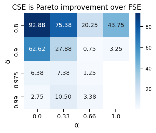
Figure 1: Percentage of instances in which the CSE Pareto is a Pareto improvement over the corresponding FSE for different combinations of agents’ patience levels and degree of preference correlation.

The previous Pareto comparison only allows for a very high-level comparison of FS and CS. In order to better understand the conditions under which certain agents benefit from FS or CS, we evaluate how many agents are better off in CS and how many agents are better off in FS. Our numerical experiments show that all families are almost always better off in CS. We refer the reader to Appendix 14.1 for more details on families’ statistics. For children, the combination of model parameters affects which approach appears more appealing. Figure 2 shows how many children are (strictly) better off (in terms of utilities) in CS and FS for different parameter combinations.

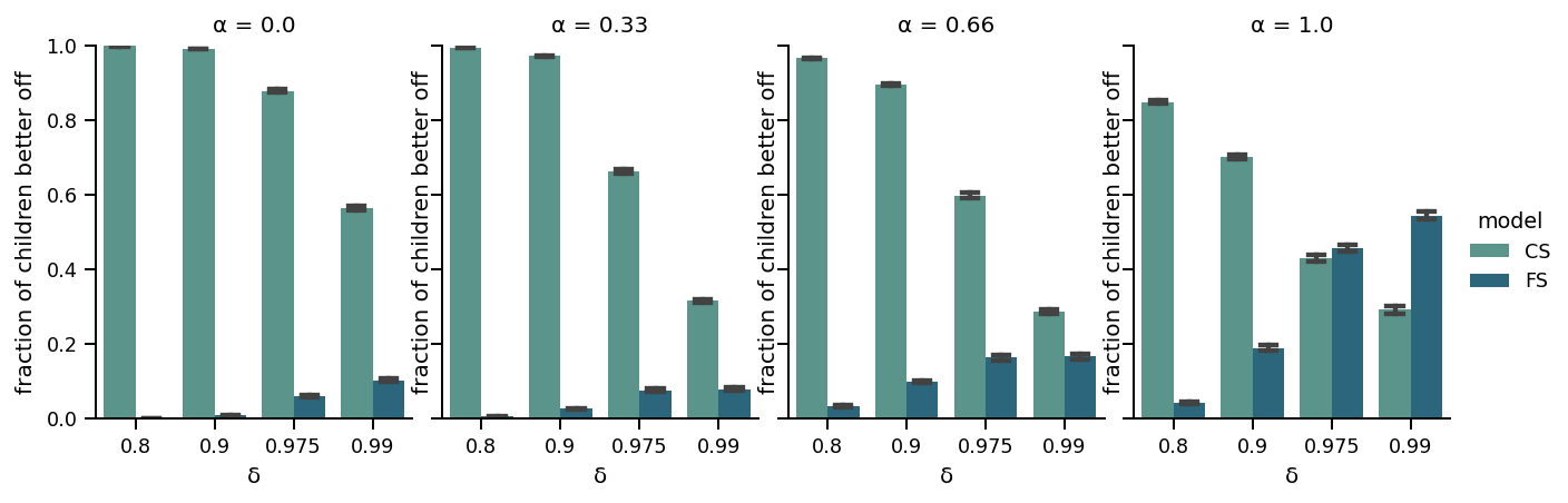
Figure 2: The ratio of children who are on average (strictly) better off in terms of utilities in either approach in the family-optimal equilibrium for different combinations of agents’ patience and the level of preference correlation.

CS provides higher utility than FS for almost all children when agents are sufficiently impatient (e.g., $\delta=0.8$) because CS allows agents to express interest in more potential match partners without risking wasted search efforts. Being interested in more agents increases the probability of getting matched at each time step, which is especially valuable to children when patience is low. On the other hand, FS incentivizes agents to focus on a smaller set of match candidates due to higher expected total search costs. When $\delta=0.8$, families will on average be interested in $35.9$ and $43.5$ child types in FS and CS, respectively. Interestingly, more children benefit from FS than CS when agents are extremely patient and agents’ preferences are almost completely aligned. This explains why CSEs are less frequently Pareto improvements over FSEs under these conditions, as we previously saw in Figure 1.

Figure 3: The ratio of children who are on average (strictly) better off in terms of (expected discounted) match value in either approach in the family-optimal equilibrium for different combinations of agents’ patience and the level of preference correlation.

Figure 3 shows that CS not only reduces wasted search efforts in many cases but also enables children to match with more preferred families. We calculate a child’s match value as the child’s utility ignoring the expected search costs, which might be less relevant to a policymaker trying to improve child outcomes.

8 Discussion and Conclusion

We are the first to apply market design principles and a formal game theoretical model to study the process by which children in the child welfare system are adopted. We introduced a novel search-and-matching model to compare two competing search paradigms. First, we analyzed the Nash equilibria of the games induced by our model. We show that agents follow novel threshold strategies as best responses, subject to a tie-breaking assumption. Also, Nash equilibria form a non-empty complete lattice in either setting.

Search frictions caused by the nature of the adoption process present one of the biggest obstacles to efficient matching efforts. We found that decreasing wasted search efforts leads to generally better outcomes, which are realized in caseworker-driven search. We explored the nuances of this finding to identify circumstances for which this intuition fails to hold.

As our main theoretical result, we showed that each caseworker-driven search equilibrium can Pareto dominate all family-driven search equilibria, but no equilibrium of family-driven search can ever Pareto dominate any caseworker-driven search equilibrium. Despite less wasted search efforts, caseworker-driven search equilibria do not always Pareto dominate those of family-driven search. However, we numerically investigated a wide range of underlying model parameters to observe that caseworker-driven search is better for most agents.

These results suggest that adoption agencies should consider using search technologies that allow caseworkers to perform a targeted search, rather than a strategy of broad announcements to which families respond. In our interviews with a North American adoption agency, managers have indicated to us that practices resembling family-driven search have dominated practice, although some have more recently switched to adopt a new technology resembling caseworker-driven search. Our results help to rationalize this decision and understand the advantages of caseworker-driven search.

Furthermore, we identified environments in which such a switch from family-driven to caseworker-driven search would be not be desirable. In only the case when agents are very patient and preferences are highly correlated, we found numerically that a majority of children are worse off in caseworker-driven search. Families display a willingness to wait for their chance to match with a child they prefer. However, we know from domain experts that especially families’ patience is limited in practice, as their wish to adopt a child is usually very strong after completing the strenuous process of a home study investigation. We also proved that in such cases — i.e., if families are sufficiently impatient — all children are unambiguously better off in caseworker-driven search compared to family-driven search, regardless of correlation in preferences. Moreover, agents’ preferences are far from being highly correlated in practice. Domain experts report idiosyncratic preferences of families based on different characteristics of children such as ethnicity, gender, or age.

Our model has some limitations. The instant replacement assumption is a theoretical abstraction. Elimination of this assumption requires a model with a large state space, which compromises its tractability. Instead, we introduced the market thickness indicator to soften this assumption. Also, having a single match success probability $p$ is a simplification of a rather idiosyncratic process that involves possible revelation of private information. In the end, we isolated the main similar and contrasting features of these search processes and created a tractable model that incorporates the most important market-level aspects of the adoption process.

Although further empirical field studies are required, our results have the potential to consider replacing the main search paradigm in adoption, family-driven search, with newer caseworker-driven search technology. Such a fundamental shift in the child adoption matching process requires that powerful search and matching tools be widely available for caseworkers. Our findings motivate future research on the development of better recommendation systems using machine learning and matching theory to help caseworkers search for suitable families more efficiently.

We thank the adoption caseworkers and managers who provided valuable insights about the search and matching process. This paper is part of a project that has received funding from the European Research Council (ERC) under the European Union’s Horizon 2020 research and innovation programme (Grant agreement No. 805542).

9 Descriptions of Approaches to Adoption Matching

In this section, we give a more detailed introduction to how matches between children and families are formed in practice under the two approaches.

9.1 Family-driven Search

A child welfare agency might send an email to announce a child’s availability and invite families to respond if interested. The child might have just entered the foster care system and is thus announced for the first time, or has been announced before but no suitable match had been identified. The announcement contains basic information about the child. If families are interested in learning more about the child, they contact the adoption agency. The caseworker responsible for the child compiles a list of interested families. In most jurisdictions, a caseworker is obligated to seriously consider each family that has shown interest. The caseworker then begins investigating those families to determine which family is the best suitable match. The caseworker might reject some families immediately, while promising candidates require further investigation through reading the family’s home study and conducting interviews. This process of determining the final match suitability is usually time consuming for both sides and emotionally stressful for families. Finally, the child can be placed with the most suitable family or remain unmatched.

9.2 Caseworker-driven Search

Caseworkers have access to an advanced software tool that enables them to efficiently browse through prospective parents that registered with the agency. After having selected a case (i.e., a child), the caseworker sees a curated list of families with promising match candidates for that child showing up at the top. The caseworker then decides which of these families to investigate and in which order. Investigation means that the caseworker looks at the family’s profile, reads their home study, and interviews the family. As in family-driven search, this process is often time consuming for both sides and emotionally stressful for families. If a contacted family turns out to be a suitable match for the child, the match proceeds to placement. If not, the caseworker can either move on to the next family or temporarily stop the search if there are no promising families remaining. The search resumes some time in the future, as caseworkers are responsible for multiple children, and have other responsibilities besides identifying matches. Therefore, if no match has been identified, a caseworker might only work on the same case after a couple of weeks or even months.

10 Additional Lemmas and Propositions

10.1 Proposition 10.1

Here, we show that processing families in decreasing order of $v_{c}(f)$ is optimal for children in CS.

Proposition 10.1

In CS, $c$’s utility is maximized if the caseworker processes families in decreasing order of $v_{c}({f})$.

Proof 10.2

Proof. Assume child $c$ is active at the current time step. Note that families without interest in $c$ do not affect $c$’s utility in any way. For the remaining families, $c$ faces a Pandora’s box problem (Weitzman 1979) where $c$ receives a payoff of $v_{c}({f})$ with probability $p$ and a payoff of 0 with probability $1-p$ when the box corresponding to family $f$ is opened. Notice that the reservation value of the box corresponding to family $f$ is higher than for family $f^{\prime}$ if and only if $v_{c}({f})>v_{c}({f^{\prime}})$.

10.2 Proposition 10.3

Strategy $s_{f}$ is a simple threshold strategy with threshold $z\in\mathbb{R}$ for family $f$ if $s_{f}=\mathbbm{1}[v_{f}({c})\geq z]$, $\forall c\in C$. Here, we show that there exist instances where families cannot best respond with a simple threshold strategy.

Proposition 10.3

In FS, there exists an instance with a family $f$ and other agents’ strategies $s_{-f}$, such that no simple threshold strategy $s_{f}$ is a best response for $f$.

Proof 10.4

Proof. Consider the following example: Let $C=\{c_{1},c_{2}\}$, $F=\{f_{1},f_{2}\}$ and let valuations be according to the following tables for some $\epsilon>0$.

$v_{c}({f})$	$f_{1}$	$f_{2}$
$c_{1}$	1	$1-\epsilon$
$c_{2}$	1	$1-\epsilon$

$v_{f}({c})$	$f_{1}$	$f_{2}$
$c_{1}$	1	1
$c_{2}$	$1-\epsilon$	$1-\epsilon$

Suppose strategy profile $s$ is such that $s_{c}(f)=s_{f}(c)=1$ for all $c\in C$, $f\in F$. If $\epsilon$ is small enough and $(1-\lambda p)p<\kappa_{F}\leq p$, then it is optimal for $f_{2}$ to only be interested in $c_{2}$, even though $f_{2}$ strictly prefers $c_{1}$.

11 Remaining Proofs

11.1 Proof of Proposition 3.1

In FS, one way to express $c$’s utility is as follows:

$$u^{FS}_{c}(s)=\Bigg{[}1-\lambda p\sum_{f\in M_{c}(s)}\beta_{cf}(s)\Bigg{]}\delta_{C}u^{FS}_{c}(s)+\lambda\sum_{f\in M_{c}(s)}\Big{[}\beta_{cf}(s)pv_{c}({f})-\kappa_{C}\Big{]}.$$ (24)

The probability of a match forming between $c$ and $f$ at the current time step is $\lambda p\beta_{cf}(s)$ if there is mutual interest, in which case $c$ obtains a value of $v_{c}(f)$ and leaves the process. For any active family that showed interest, $c$ incurs search costs $\kappa_{C}$. If $c$ remains unmatched, then $c$ receives $\delta_{C}u^{FS}_{c}(s)$. By pulling $\delta_{C}u^{FS}_{c}(s)$ out of the sums, we get

$$u^{FS}_{c}(s)=\delta_{C}u^{FS}_{c}(s)+\lambda\sum_{f\in M_{c}(s)}\Big{(}\beta_{cf}(s)p\big{(}v_{c}({f})-\delta_{C}u^{FS}_{c}(s)\big{)}-\kappa_{C}\Big{)}.$$ (25)

The proof for families’ utilities in FS and agents’ utilities in CS is analogous and omitted.

11.2 Proof of Proposition 4.2

First of all, notice that whether agent $i$ is interested in some agent $j$ or not does not affect agent $i$’s utility if $j$ is not interested in $i$. Further, for an arbitrary family $f$ in FS, $\beta_{cf}(s)$ does not depend on $s_{f}$. By slightly modifying Equation 6, we can see that when $f$ plays a best response in $s$ it must hold that

$$u^{FS*}_{c}(s_{-f})=\delta_{F}u^{FS*}_{c}(s_{-f})+\frac{1}{n}\sum_{c\in M_{f}(s)}\Big{(}\beta_{cf}(s)p\big{(}v_{f}({c})-\delta_{F}u^{FS*}_{c}(s_{-f})\big{)}-\kappa_{F}\Big{)}.$$ (26)

By Equation 26 it must hold for all $c\in C$ that

$$s_{f}(c)=\mathbbm{1}[\beta_{cf}(s)p\big{(}v_{c}({f})-\delta_{F}u^{FS*}_{f}(s_{-f})\big{)}\geq\kappa_{F}]$$ (27)

when there is mutual interest between $c$ and $f$, as $s_{f}$ would otherwise not be a best response. That is, because all children $c$ contribute non-negatively to $f$’s utility if and only if $\beta_{cf}(s)p\big{(}v_{c}({f})-\delta_{F}u^{FS*}_{f}(s_{-f})\big{)}\geq\kappa_{F}$. By our tie-breaking assumption, the claim of the proposition follows for families in FS. The proof for families in CS is analogous and thus omitted.

In the remainder of the proof, we show that the statement holds for children in FS. The proof for CS is again analogous and therefore omitted. Let $c$ be an arbitrary child. For a best response $s_{c}$ to $s_{-c}$ we have that

$$u^{FS*}_{c}(s_{-c})=\delta_{C}u^{FS*}_{c}(s_{-c})+\lambda\sum_{f\in F}s_{c}(f)s_{f}(c)\Big{(}\beta_{cf}(s)p\big{(}v_{c}({f})-\delta_{C}u^{FS*}_{c}(s_{-c})\big{)}-\kappa_{C}\Big{)}.$$ (28)

As for families, it must be the case that

$$s_{c}(f)=\mathbbm{1}[\beta_{cf}(s)p\big{(}v_{c}({f})-\delta_{C}u^{FS*}_{c}(s_{-c})\big{)}\geq\kappa_{C}]$$ (29)

because for all $f,f^{\prime}\in F$

$$\beta_{cf}(s)\geq\beta_{cf^{\prime}}(s)\iff v_{c}({f})\geq v_{c}({f^{\prime}}),$$ (30)

and otherwise $s_{c}$ would not be a best response to $s_{-c}$. Again, by our tie-breaking assumption the claim of the proposition follows for children in FS.

11.3 Proof of Proposition 4.5 (Part for CS)

For CS, we define a mapping $T^{CS}:Y\rightarrow Y$ as follows: $T^{CS}=(T^{CS}_{i})_{i\in A}$, where

$$T^{CS}_{c}(y)=\delta_{C}y_{c}+\lambda\sum_{f\in F}\mathbbm{1}[p(v_{f}({c})-\delta_{F}y_{f})\geq\kappa_{F}]\beta_{cf}(y)\Big{(}p(v_{c}({f})-\delta_{C}y_{c})-\kappa_{C}\Big{)}^{+}$$ (31)

for all $c\in C$ and

$$T^{CS}_{f}(y)=\delta_{F}y_{f}+\frac{1}{n}\sum_{c\in C}\mathbbm{1}[p(v_{c}({f})-\delta_{C}y_{c})\geq\kappa_{C}]\beta_{cf}(y)\Big{(}p(v_{f}({c})-\delta_{F}y_{f})-\kappa_{F}\Big{)}^{+}.$$ (32)

for all $f\in F$. Note that any fixed point of $T^{CS}$ is an equilibrium threshold profile in CS. We now show that $T^{CS}$ is monotonically increasing according to $\leq_{C}$. Let $c\in C$, $y,y^{\prime}\in Y$, and $y\leq_{C}y^{\prime}$. It holds that

$$T^{CS}_{c}(y) =\delta_{C}y_{c}+\lambda\sum_{f\in F}\mathbbm{1}[p(v_{f}({c})-\delta_{F}y_{f})\geq\kappa_{F}]\beta_{cf}(y)\Big{(}p(v_{c}({f})-\delta_{C}y_{c})-\kappa_{C}\Big{)}^{+}$$ (33)

$$\leq\delta_{C}y^{\prime}_{c}+\lambda\sum_{f\in F}\mathbbm{1}[p(v_{f}({c})-\delta_{F}y^{\prime}_{f})\geq\kappa_{F}]\beta_{cf}(y^{\prime})\Big{(}p(v_{c}({f})-\delta_{C}y^{\prime}_{c})-\kappa_{C}\Big{)}^{+}$$ (34)

$$=T^{CS}_{c}(y^{\prime}),$$ (35)

because each family is weakly less selective under $s(y^{\prime})$ than $s(y)$.

Similarly, since each child is weakly more selective under $s(y^{\prime})$ than $s(y)$, we have for all $f\in F$

$$T^{CS}_{f}(y) =\delta_{F}y_{f}+\frac{1}{n}\sum_{c\in C}\mathbbm{1}[p(v_{c}({f})-\delta_{C}y_{c})\geq\kappa_{C}]\beta_{cf}(y)\Big{(}p(v_{f}({c})-\delta_{F}y_{f})-\kappa_{F}\Big{)}^{+}$$ (36)

$$\geq\delta_{F}y^{\prime}_{f}+\frac{1}{n}\sum_{c\in C}\mathbbm{1}[p(v_{c}({f})-\delta_{C}y_{c})\geq\kappa_{C}]\beta_{cf}(y^{\prime})\Big{(}p(v_{f}({c})-\delta_{F}y^{\prime}_{f})-\kappa_{F}\Big{)}^{+}$$ (37)

$$=T^{CS}_{f}(y^{\prime}).$$ (38)

Note that $T^{CS}$ maps elements from $Y$ to $Y$ and $(Y,\leq_{C})$ is a complete lattice. By Tarski’s fixed point theorem, the claim for CS follows.

11.4 Proof of Proposition 6.5

Let $u=(u_{i}(s^{co-CS,\lambda}))_{i\in A}$ denote the vector of agents’ utilities under $s^{co-CS,\lambda}$ and let $Y^{\prime}=[u_{c},\bar{v}]^{n}\times[0,u_{f}]^{m}\subseteq[0,\bar{v}]^{n+m}=Y$. We now define a mapping $T^{\lambda}:Y\rightarrow Y$ as follows: $T^{\lambda}=(T^{\lambda}_{i})_{i\in A}$, where

$$T^{\lambda}_{c}(y)=\delta_{C}y_{c}+\lambda\sum_{f\in F}\mathbbm{1}[p(v_{f}({c})-\delta_{F}y_{f})\geq\kappa_{F}]\beta_{cf}(y)\Big{(}p(v_{c}({f})-\delta_{C}y_{c})-\kappa_{C}\Big{)}^{+}$$ (39)

for all $c\in C$ and

$$T^{\lambda}_{f}(y)=\delta_{F}y_{f}+\frac{1}{n}\sum_{c\in C}\mathbbm{1}[p(v_{c}({f})-\delta_{C}y_{c})\geq\kappa_{C}]\beta_{cf}(y)\Big{(}p(v_{f}({c})-\delta_{F}y_{f})-\kappa_{F}\Big{)}^{+}.$$ (40)

As we have seen in a previous proof, $T^{\lambda}$ is $\leq_{C}$-monotone on $Y$. We now show that $T^{\lambda^{\prime}}$ maps from $Y^{\prime}$ to $Y^{\prime}$, which by Tarski’s fixed-point theorem yields the result. Since $T^{\lambda}$ is $\leq_{C}$-monotone and $u$ is the $\leq_{C}$-minimal element of $Y^{\prime}$, it is sufficient to show that $T^{\lambda^{\prime}}(u)\in Y^{\prime}$.

Because $u$ is an equilibrium threshold profile, we have that $T^{\lambda}(u)=u\in Y^{\prime}$. Further, it can easily be verified that $T^{\lambda}(y)\leq_{C}T^{\lambda^{\prime}}(y)$ for all $y\in Y$. Hence, $T^{\lambda^{\prime}}(u)\in Y^{\prime}$, which completes the proof.

12 Algorithm to Compute FS-TSs from Threshold Profiles

Algorithm 1 can be used to compute $s^{FS}(y)$ for a given threshold profile $y\in\mathbb{R}^{n+m}$. Since $\beta_{cf}(s)$ only depends on families $f^{\prime}\in F$ with $v_{c}({f^{\prime}})>v_{c}({f})$ and for each child families are processed in decreasing order of $v_{c}({f})$, the final strategy profile satisfies the equations for FS from Proposition 3.1.

Input: $y\in\mathbb{R}^{n+m}$

Output: Strategy profile $s\in S$

$s_{c}(f):=0$ and $s_{f}(c):=0$ for all $c\in C$, $f\in F$

for $c\in C$ do

      $U:=F$

     while $U\neq\emptyset$ do

           $f:=\arg\max_{f^{\prime}\in U}v_{c}({f^{\prime}})$

          if $\beta_{cf}(s)p(v_{f}({c})-\delta_{F}y_{f})\geq\kappa_{F}$ then

                $s_{f}(c):=1$

                end if

               if $\beta_{cf}(s)p(v_{c}({f})-\delta_{C}y_{c})\geq\kappa_{C}$ then

                     $s_{c}(f):=1$

                     end if

                    $U:=U\setminus\{f\}$

                     end while

                    

                     end for

Algorithm 1 Thresholds to strategy profile

13 Limit Results

Here, we provide a collection of limit results that all illustrate how the differences between FS and CS disappear as certain parameters take on extreme values.

13.1 Negligible Search Costs

The next proposition shows that the games induced by CS and FS become identical as search costs become negligible.

Proposition 13.1

As $\kappa_{C}\rightarrow 0$ and $\kappa_{F}\rightarrow 0$, $|u^{FS}_{i}(s)-u^{CS}_{i}(s)|\rightarrow 0$ for all $s\in S$, $i\in A$.

Proof 13.2

Proof. Assume that $\kappa_{C}=\kappa_{F}=:\kappa$ and let $s\in S$. For each family $f$, define $T_{s,f}^{FS}:Y\rightarrow\mathbb{R}$ and $T_{s,f}^{CS}:Y\rightarrow\mathbb{R}$ as follows:

$$T_{s,f}^{FS}(y)=\delta_{F}y_{f}+\frac{1}{n}\sum_{c\in C}s_{c}(f)s_{f}(c)\Big{(}\beta_{cf}(s)p(v_{f}({c})-\delta_{F}y_{f})-\kappa\Big{)}$$ (41)

and

$$T_{s,f}^{CS}(y)=\delta_{F}y_{f}+\frac{1}{n}\sum_{c\in C}s_{c}(f)s_{f}(c)\beta_{cf}(s)\Big{(}p(v_{f}({c})-\delta_{F}y_{f})-\kappa\Big{)}.$$ (42)

Similarly, for all $c\in C$, let

$$T_{s,c}^{FS}(y)=\delta_{C}y_{c}+\lambda\sum_{f\in F}s_{c}(f)s_{f}(c)\Big{(}\beta_{cf}(s)p(v_{c}({f})-\delta_{C}y_{c})-\kappa\Big{)}$$ (43)

and

$$T_{s,c}^{CS}(y)=\delta_{C}y_{c}+\lambda\sum_{f\in F}s_{c}(f)s_{f}(c)\beta_{cf}(s)\Big{(}p(v_{c}({f})-\delta_{C}y_{c})-\kappa\Big{)}.$$ (44)

Notice that the unique fixpoints $y^{FS},y^{CS}\in Y$ of $T_{s}^{FS}(y)$ and $T_{s}^{CS}(y)$ define agents’ utilities under $s$ in FS and CS, respectively. For all $y\in Y$ and $f\in F$ it holds that

$$\lim_{\kappa\rightarrow 0}\left(\delta_{F}y_{f}+\frac{1}{n}\sum_{c\in C}s_{c}(f)s_{f}(c)\Big{(}\beta_{cf}(s)p(v_{f}({c})-\delta_{F}y_{f})-\kappa\Big{)}\right)$$ (45)

$$= \delta_{F}y_{f}+\frac{1}{n}\sum_{c\in C}s_{c}(f)s_{f}(c)\Big{(}\beta_{cf}(s)p(v_{f}({c})-\delta_{F}y_{f})\Big{)}$$ (46)

$$= \lim_{\kappa\rightarrow 0}\left(\delta_{F}y_{f}+\frac{1}{n}\sum_{c\in C}s_{c}(f)s_{f}(c)\beta_{cf}(s)\Big{(}p(v_{f}({c})-\delta_{F}y_{f})-\kappa\Big{)}\right).$$ (47)

Similarly, for all $y\in Y$ and $c\in C$ we have that

$$\lim_{\kappa\rightarrow 0}\left(\delta_{C}y_{c}+\lambda\sum_{f\in F}s_{c}(f)s_{f}(c)\Big{(}\beta_{cf}(s)p(v_{c}({f})-\delta_{C}y_{c})-\kappa\Big{)}\right)$$ (48)

$$= \delta_{C}y_{c}+\lambda\sum_{f\in F}s_{c}(f)s_{f}(c)\Big{(}\beta_{cf}(s)p(v_{c}({f})-\delta_{C}y_{c})\Big{)}$$ (49)

$$= \lim_{\kappa\rightarrow 0}\left(\delta_{C}y_{c}+\lambda\sum_{f\in F}s_{c}(f)s_{f}(c)\beta_{cf}(s)\Big{(}p(v_{c}({f})-\delta_{C}y_{c})-\kappa\Big{)}\right),$$ (50)

and hence $\lim_{\kappa\rightarrow 0}|u^{FS}_{i}(s)-u^{CS}_{i}(s)|=0$ for all $i\in A$.

FS and CS do not necessarily become identical if only one side has negligible search costs. In both cases—i.e., if only $\kappa_{C}\rightarrow 0$ or only $\kappa_{F}\rightarrow 0$—we can create instances where the sets of equilibria differ from each other in the two approaches.

13.2 High Match Success Probability and Market Thickness

Match success probability and market thickness indicator are strongly connected in our model, such that we cannot make any insightful statements about the limit behavior if only one of them approaches 1. However, if it is certain that a family of each type will be present at each time step and that each family would be a suitable match, we observe once more that FS and CS become equivalent in a slightly different way.

Proposition 13.3

As $\lambda p\rightarrow 1$, $|u^{FS}_{i}(s^{FS}(y))-u^{CS}_{i}(s^{CS}(y))|\rightarrow 0$ for all $y\in Y$, $i\in A$.

Proof 13.4

Proof. For each family $f$, define $T_{f}^{FS}:Y\rightarrow\mathbb{R}$ and $T_{f}^{CS}:Y\rightarrow\mathbb{R}$ as follows:

$$T_{f}^{FS}(y)=\delta_{F}y_{f}+\frac{1}{n}\sum_{c\in C}\mathbbm{1}[\beta^{FS}_{cf}(y)p(v_{c}({f})-\delta_{C}y_{c})\geq\kappa_{C}]\Big{(}\beta^{FS}_{cf}(y)p(v_{f}({c})-\delta_{F}y_{f})-\kappa_{F}\Big{)}^{+}$$ (51)

and

$$T_{f}^{CS}(y)=\delta_{F}y_{f}+\frac{1}{n}\sum_{c\in C}\mathbbm{1}[p(v_{c}({f})-\delta_{C}y_{c})\geq\kappa_{C}]\beta^{CS}_{cf}(y)\Big{(}p(v_{f}({c})-\delta_{F}y_{f})-\kappa_{F}\Big{)}^{+}.$$ (52)

Similarly, for all $c\in C$, let

$$T_{c}^{FS}(y)=\delta_{C}y_{c}+\lambda\sum_{f\in F}\mathbbm{1}[\beta^{FS}_{cf}(y)p(v_{f}({c})-\delta_{F}y_{f})\geq\kappa_{F}]\Big{(}\beta^{FS}_{cf}(y)p(v_{c}({f})-\delta_{C}y_{c})-\kappa_{C}\Big{)}^{+}$$ (53)

and

$$T_{c}^{CS}(y)=\delta_{C}y_{c}+\lambda\sum_{f\in F}\mathbbm{1}[p(v_{f}({c})-\delta_{F}y_{f})\geq\kappa_{F}]\beta^{CS}_{cf}(y)\Big{(}p(v_{c}({f})-\delta_{C}y_{c})-\kappa_{C}\Big{)}^{+}.$$ (54)

Notice that the unique fixpoints $y^{FS},y^{CS}\in Y$ of $T^{FS}(y)$ and $T^{CS}(y)$ define agents’ utilities under an FS-TS and CS-TS with threshold $y$ in FS and CS, respectively. For all $y\in Y$ and $f\in F$, it holds that

$$\lim_{\lambda p\rightarrow 1}\left(\delta_{F}y_{f}+\frac{1}{n}\sum_{c\in C}\mathbbm{1}[\beta^{FS}_{cf}(y)p(v_{c}({f})-\delta_{C}y_{c})\geq\kappa_{C}]\Big{(}\beta^{FS}_{cf}(y)p(v_{f}({c})-\delta_{F}y_{f})-\kappa_{F}\Big{)}^{+}\right)$$ (55)

$$= \delta_{F}y_{f}+\frac{1}{n}\sum_{c\in C}\mathbbm{1}\left[f=\argmax_{f^{\prime}\in F:v_{f^{\prime}}({c})-\delta_{F}y_{f^{\prime}}>\kappa_{F}\land v_{c}({f^{\prime}})-\delta_{C}y_{c}>\kappa_{C}}v_{c}({f^{\prime}})\right]\Big{(}v_{f}({c})-\delta_{F}y_{f}-\kappa_{F}\Big{)}$$ (56)

$$= \lim_{\lambda p\rightarrow 1}\left(\delta_{F}y_{f}+\frac{1}{n}\sum_{c\in C}\mathbbm{1}[\beta^{CS}_{cf}(y)p(v_{c}({f})-\delta_{C}y_{c})\geq\kappa_{C}]\beta^{CS}_{cf}(y)\Big{(}p(v_{f}({c})-\delta_{F}y_{f})-\kappa_{F}\Big{)}^{+}\right).$$ (57)

Similarly, for all $y\in Y$ and $c\in C$ we have that

$$\lim_{\lambda p\rightarrow 1}\left(\delta_{C}y_{c}+\lambda\sum_{f\in F}\mathbbm{1}[\beta^{FS}_{cf}(y)p(v_{f}({c})-\delta_{F}y_{f})\geq\kappa_{F}]\Big{(}\beta^{FS}_{cf}(y)p(v_{c}({f})-\delta_{C}y_{c})-\kappa_{C}\Big{)}^{+}\right)$$ (58)

$$= \delta_{C}y_{c}+\lambda\sum_{f\in F}\mathbbm{1}\left[f=\argmax_{f^{\prime}\in F:v_{f^{\prime}}({c})-\delta_{F}y_{f^{\prime}}>\kappa_{F}\land v_{c}({f^{\prime}})-\delta_{C}y_{c}>\kappa_{C}}v_{c}({f^{\prime}})\right]\Big{(}v_{c}({f})-\delta_{C}y_{c}-\kappa_{C}\Big{)}$$ (59)

$$= \lim_{\lambda p\rightarrow 1}\left(\delta_{C}y_{c}+\lambda\sum_{f\in F}\mathbbm{1}[p(v_{f}({c})-\delta_{F}y_{f})\geq\kappa_{F}]\beta^{CS}_{cf}(y)\Big{(}p(v_{c}({f})-\delta_{C}y_{c})-\kappa_{C}\Big{)}^{+}\right).$$ (60)

and hence $\lim_{\lambda p\rightarrow 1}|u_{i}(s^{FS}_{i}(y))-u_{i}(s^{CS}_{i}(y))|=0$. This concludes the proof for families. For children, the proof is analogous and omitted.

In order to see why Proposition 13.3 holds, notice that the probability of child $c$ matching with his first choice from $M_{c}(s)$ goes to 1 as $\lambda p\rightarrow 1$. Thus, the contribution of all other families from $M_{c}(s)$ goes to zero. As only these first choices contribute to utilities, the difference between FS and CS again disappears.

13.3 Low Market Thickness

As the supply on the family side becomes very small, the differences between CS and FS disappear in equilibrium.

Proposition 13.5

As $\lambda\rightarrow 0$, $|u^{FS}_{i}(s)-u^{CS}_{i}(s)|\rightarrow 0$ for all $s\in S$, $i\in A$.

Proof 13.6

Proof. Notice that the unique fixpoints $y^{FS},y^{CS}\in Y$ of $T_{s}^{FS}(y)$ and $T_{s}^{CS}(y)$ (recall definitions from the proof of Proposition 13.1 define agents’ utilities under $s$ in FS and CS, respectively. For all $y\in Y$ and $f\in F$ it holds that

$$\lim_{\lambda\rightarrow 0}\left(\delta_{F}y_{f}+\frac{1}{n}\sum_{c\in C}s_{c}(f)s_{f}(c)\Big{(}\beta_{cf}(s)p(v_{f}({c})-\delta_{F}y_{f})-\kappa_{F}\Big{)}\right)$$ (61)

$$= \delta_{F}y_{f}+\frac{1}{n}\sum_{c\in C}s_{c}(f)s_{f}(c)\Big{(}p(v_{f}({c})-\delta_{F}y_{f})\Big{)}$$ (62)

$$= \lim_{\lambda\rightarrow 0}\left(\delta_{F}y_{f}+\frac{1}{n}\sum_{c\in C}s_{c}(f)s_{f}(c)\beta_{cf}(s)\Big{(}p(v_{f}({c})-\delta_{F}y_{f})-\kappa_{F}\Big{)}\right),$$ (63)

because $\beta_{cf}(s)\rightarrow 1$ as $\lambda\rightarrow 0$. Similarly, for all $y\in Y$ and $c\in C$ we have that

$$\lim_{\lambda\rightarrow 0}\left(\delta_{C}y_{c}+\lambda\sum_{f\in F}s_{c}(f)s_{f}(c)\Big{(}\beta_{cf}(s)p(v_{c}({f})-\delta_{C}y_{c})-\kappa_{C}\Big{)}\right)$$ (64)

$$= \delta_{C}y_{c}$$ (65)

$$= \lim_{\lambda\rightarrow 0}\left(\delta_{C}y_{c}+\lambda\sum_{f\in F}s_{c}(f)s_{f}(c)\beta_{cf}(s)\Big{(}p(v_{c}({f})-\delta_{C}y_{c})-\kappa_{C}\Big{)}\right),$$ (66)

and hence $\lim_{\lambda\rightarrow 0}|u^{FS}_{i}(s)-u^{CS}_{i}(s)|=0$ for all $i\in A$.

The reason why the statement holds is that for very small $\lambda$ families do not have to worry about competition in FS, as it is likely that there is no other family active at any given time step.

13.4 Patient Agents

Here, we first need to revisit classical matching markets. The matching market induced by $(v,\delta_{C},\delta_{F},\kappa_{C},\kappa_{F},p,\lambda)$ is a tuple $(C,F,\succ)$, where $f\succ_{c}f^{\prime}$ if and only if $v_{c}({f})>v_{c}({f^{\prime}})$ and $c\succ_{f}c^{\prime}$ if and only if $v_{f}({c})>v_{f}({c^{\prime}})$. Further, $f\succ_{c}c$ if and only if $pv_{c}({f})\geq\kappa_{C}$ and $c\succ_{f}f$ if and only if $pv_{f}({c})\geq\kappa_{F}$. For the remainder of this section, we assume that $\delta_{C}=\delta_{F}=:\delta$.

Proposition 13.7

There exists $\bar{\delta}\in[0,1)$, such that for all $\delta\in[\bar{\delta},1)$ the set of equilibrium matching correspondences are identical in FS and CS and coincide with the set of stable matchings in the induced marriage market.

For small $p$ and large search costs, the statement above is trivial: If search costs become too large or the probability of a match being suitable becomes too small, no agent will have an incentive to be interested in any potential match candidate in either FS or CS. Hence, no matches will form in any equilibrium.

We only prove the statement for iii) here, as i) and ii) are trivial. For this proof, we first need to revisit classical matching markets. The matching market induced by $(v,\delta_{C},\delta_{F},\kappa_{C},\kappa_{F},p,\lambda)$ is a tuple $(C,F,\succ)$, where $f\succ_{c}f^{\prime}$ if and only if $v_{c}({f})>v_{c}({f^{\prime}})$ and $c\succ_{f}c^{\prime}$ if and only if $v_{f}({c})>v_{f}({c^{\prime}})$. Further, $f\succ_{c}c$ if and only if $pv_{c}({f})\geq\kappa_{C}$ and $c\succ_{f}f$ if and only if $pv_{f}({c})\geq\kappa_{F}$.

Let $(C,F,\succ)$ be a matching market where agents have strict preferences.

Definition 13.8

A pair of functions $g=(g_{C},g_{F})$ is called a pre-matching if $g_{C}:C\rightarrow A$ and $g_{F}:F\rightarrow A$, such that if $g_{C}(c)\neq c$ then $g_{C}(c)\in F$ and if $g_{F}(f)\neq f$ then $g_{F}(f)\in C$.

We say that a pre-matching $g$ induces a matching $w$ if the function $w:A\rightarrow A$ defined by $w(i)=g(i)$ is a matching. Consider the following set of equations:

$$g_{C}(c)=\max_{\succ_{c}}\left(\{f\in F\mid c\succeq_{f}g_{F}(f)\}\cup\{c\}\right),\quad c\in C,$$ (67)

$$g_{F}(f)=\max_{\succ_{f}}\left(\{c\in C\mid f\succeq_{c}g_{C}(c)\}\cup\{f\}\right),\quad f\in F,$$ (68)

where the maxima are taken with respect to agents’ preferences.

Lemma 13.9 (Adachi (2003))

If a matching $w$ is stable, then the pre-matching $g$ defined by $w$ solves the above equations. If a pre-matching $g$ solves the above equations, then $g$ induces a stable matching $w$.

With the above lemma, we can now prove Lemma 13.10. Assume that $\delta_{C}=\delta_{F}=:\delta$.

Lemma 13.10

There exists $\bar{\delta}\in[0,1)$, such that for all $\delta\in[\bar{\delta},1)$ the set of equilibrium matching correspondences are identical in FS and CS and coincide with the set of stable matchings in the induced marriage market.

Proof 13.11

Proof. Let $s\in S^{FS}$ and $c\in C$. $c$’s utility under $s$ is the unique value $u^{FS}_{c}(s)$ that satisfies

$$u_{c}(s)=\delta u_{c}(s)+\lambda\sum_{f\in F}s_{f}(c)\Big{(}\beta_{cf}(s)p(v_{f}({c})-\delta u_{c}(s))-\kappa_{C}\Big{)}^{+}$$ (69)

$$\iff (1-\delta)u_{c}(s)=\lambda\sum_{f\in F}s_{f}(c)\Big{(}\beta_{cf}(s)p(v_{f}({c})-\delta u_{c}(s))-\kappa_{C}\Big{)}^{+}.$$ (70)

Therefore, as $\delta\rightarrow 1$ we get

$$\frac{1}{n}\sum_{f\in F}s_{f}(c)\Big{(}\beta_{cf}(s)p(v_{f}({c})-\delta u^{FS}_{c}(s))-\kappa_{C}\Big{)}^{+}\rightarrow 0.$$ (71)

For the sake of contradiction, assume that $|M_{c}(s)|\geq 2$. Let $f^{*}=\arg\max_{f\in F:s_{f^{*}}(c)=1}v_{c}({f})$ and $f\in M_{c}(s)\setminus\{f^{*}\}$. Because of Equation 71, it must hold that

$$\beta_{cf}(s)\Big{(}v_{c}({f})-\delta u_{c}(s)-\kappa_{C}/p\Big{)}^{+}\rightarrow 0.$$ (72)

However, since $v_{c}(f^{*})>v_{c}({f})$ and $\beta_{cf^{*}}(s)>\beta_{cf}(s)$ we get that

$$\beta_{cf^{*}}(s)\Big{(}v_{c}({f^{*}})-\delta u_{c}(s)-\kappa_{C}/p\Big{)}^{+}\rightarrow\epsilon$$ (73)

for some $\epsilon>0$, a contradiction. Hence, $M_{c}(s)=\{f^{*}\}$ if $pv_{c}({f^{*}})\geq\kappa_{C}$ or $M_{c}(s)=\emptyset$ otherwise. Notice that this is equivalent to the expression of Equation 67. Now that we have established that children will be mutually interested in at most one family, the same can similarly be shown for families, which completes the proof for FS. The proof for CS is analogous and thus omitted.

14 Numerical Evaluation: Supplementary Material

14.1 Families

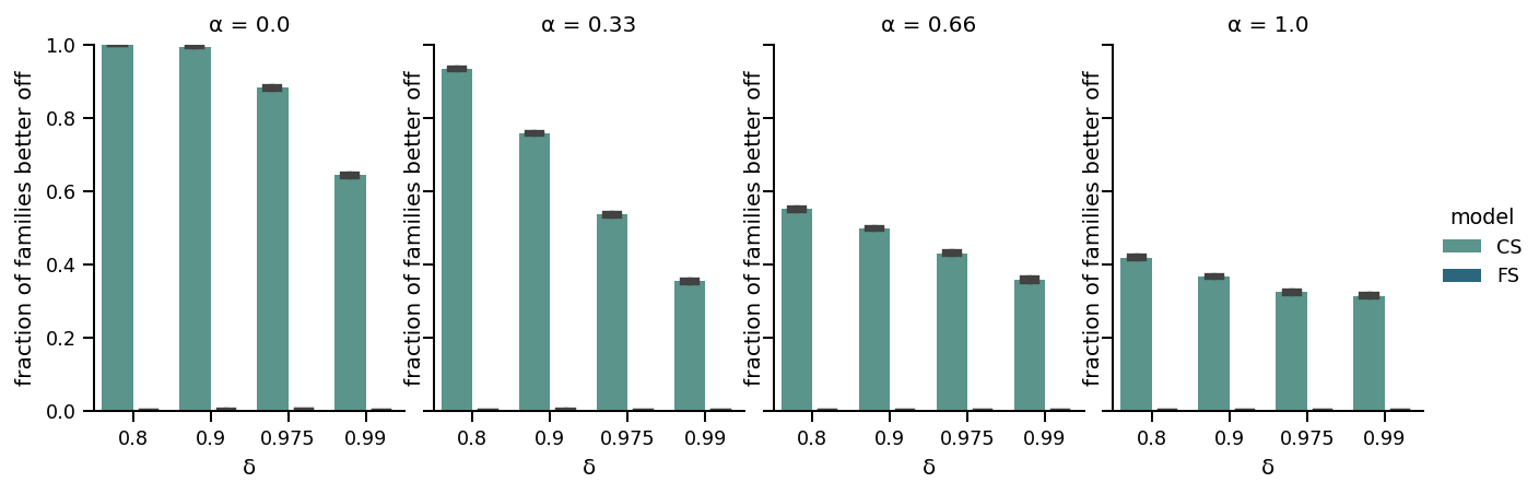
Figure 4: The ratio of families that are on average (strictly) better off in either approach in the family-optimal equilibrium for different combinations of agents’ patience and the level of preference correlation.

From Figure 4, we can see that the majority of families achieves a higher utility under CS, and almost no families achieve a higher utility under FS.

14.2 Match Probabilities

Figure 5 shows that on average children are more likely to get matched in CS than FS at any given time step.

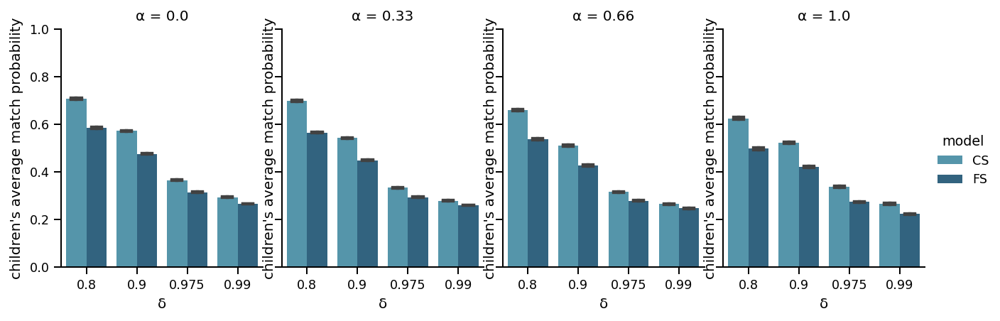
Figure 5: Children’s average match probability (averaged over all children and over all instances) in the family-optimal equilibrium for different combinations of agents’ patience and the level of preference correlation.

References

- Abdulkadiroğlu et al. (2015) Abdulkadiroğlu A, Che YK, Yasuda Y (2015) Expanding “Choice” in School Choice. American Economic Journal: Microeconomics 7(1):1–42, ISSN 1945-7669, 1945-7685, URL http://dx.doi.org/10.1257/mic.20120027.
- Adachi (2003) Adachi H (2003) A search model of two-sided matching under nontransferable utility. Journal of Economic Theory 113(2):182–198, ISSN 00220531, URL http://dx.doi.org/10.1016/S0022-0531(03)00085-1.
- Andersson et al. (2018) Andersson T, Ehlers L, Martinello A (2018) Dynamic Refugee Matching. Working paper, Lund University, Lund, Sweden.
- Arnosti et al. (2021) Arnosti N, Johari R, Kanoria Y (2021) Managing Congestion in Matching Markets. Manufacturing & Service Operations Management ISSN 1523-4614, 1526-5498, URL http://dx.doi.org/10.1287/msom.2020.0927.
- Atakan (2006) Atakan AE (2006) Assortative Matching with Explicit Search Costs. Econometrica 74(3):667–680, ISSN 00129682, 14680262, URL http://www.jstor.org/stable/4123098.
- Baccara et al. (2014) Baccara M, Collard-Wexler A, Felli L, Yariv L (2014) Child-Adoption Matching: Preferences for Gender and Race. American Economic Journal: Applied Economics 6(3):133–158, ISSN 1945-7782, 1945-7790, URL http://dx.doi.org/10.1257/app.6.3.133.
- Baccara et al. (2015) Baccara M, Lee S, Yariv L (2015) Optimal Dynamic Matching. SSRN Electronic Journal ISSN 1556-5068, URL http://dx.doi.org/10.2139/ssrn.2641670.
- Bansak et al. (2018) Bansak K, Ferwerda J, Hainmueller J, Dillon A, Hangartner D, Lawrence D, Weinstein J (2018) Improving refugee integration through data-driven algorithmic assignment. Science 359(6373):325–329, ISSN 0036-8075, 1095-9203, URL http://dx.doi.org/10.1126/science.aao4408.
- Barth (1990) Barth RP (1990) On their own: The experiences of youth after foster care. Child & Adolescent Social Work Journal 7(5):419–440, ISSN 0738-0151, 1573-2797, URL http://dx.doi.org/10.1007/BF00756380.
- Cheremukhin et al. (2020) Cheremukhin A, Restrepo-Echavarria P, Tutino A (2020) Targeted search in matching markets. Journal of Economic Theory 185:104956, ISSN 00220531, URL http://dx.doi.org/10.1016/j.jet.2019.104956.
- Children’s Bureau (2020) Children’s Bureau (2020) The AFCARS Report: Preliminary FY2019 Estimates. Version Number: 2020-06-23.
- Combe et al. (2022) Combe J, Dur U, Tercieux O, Terrier C, Ünver MU (2022) Market design for distributional objectives in (re)assignment: An application to improve the distribution of teachers in schools. Working paper, Boston College, Department of Economics.
- Courtney et al. (2010) Courtney ME, Dworsky AL, Lee JS, Raap M (2010) Midwest evaluation of the adult functioning of former foster youth: Outcomes at ages 23 and 24 (Chapin Hall at the University of Chicago Chicago).
- Delacrétaz et al. (2020) Delacrétaz D, Kominers SD, Teytelboym A (2020) Matching Mechanisms for Refugee Resettlement. Working paper, University of Oxford, Oxford, UK.
- Eeckhout (1999) Eeckhout J (1999) Bilateral Search and Vertical Heterogeneity. International Economic Review 40(4):869–887, ISSN 0020-6598, 1468-2354, URL http://dx.doi.org/10.1111/1468-2354.00045.
- Fradkin (2017) Fradkin A (2017) Search, Matching, and the Role of Digital Marketplace Design in Enabling Trade: Evidence from Airbnb. Working paper, Boston University Questrom School of Business, URL https://www.ssrn.com/abstract=2939084.
- Gale and Sotomayor (1985) Gale D, Sotomayor M (1985) Ms. Machiavelli and the stable matching problem. The American Mathematical Monthly 92(4):261–268, ISSN 00029890, 19300972, URL http://www.jstor.org/stable/2323645.
- Gerstenzang and Freundlich (2006) Gerstenzang S, Freundlich M (2006) Finding a Fit that Will Last a Lifetime: A Guide to Connecting Adoptive Families with Waiting Children.
- Hanna and McRoy (2011) Hanna M, McRoy R (2011) Innovative Practice Approaches to Matching in Adoption. Journal of Public Child Welfare 5(1):45–66, ISSN 1554-8732, URL http://dx.doi.org/10.1080/15548732.2011.542722.
- Hitsch et al. (2010a) Hitsch GJ, Hortaçsu A, Ariely D (2010a) Matching and Sorting in Online Dating. American Economic Review 100(1):130–163, ISSN 0002-8282, URL http://dx.doi.org/10.1257/aer.100.1.130.
- Hitsch et al. (2010b) Hitsch GJ, Hortaçsu A, Ariely D (2010b) What makes you click?—Mate preferences in online dating. Quantitative Marketing and Economics 8(4):393–427, ISSN 1570-7156, 1573-711X, URL http://dx.doi.org/10.1007/s11129-010-9088-6.
- Immorlica et al. (2020) Immorlica N, Leshno J, Lo I, Lucier B (2020) Information Acquisition in Matching Markets: The Role of Price Discovery. SSRN Electronic Journal ISSN 1556-5068, URL http://dx.doi.org/10.2139/ssrn.3705049.
- Jeloudar et al. (2021) Jeloudar MY, Lo I, Pollner T, Saberi A (2021) Decentralized Matching in a Probabilistic Environment. Proceedings of the 22nd ACM Conference on Economics and Computation 635–653, URL http://dx.doi.org/10.1145/3465456.3467652, arXiv: 2106.06706.
- Kanoria and Saban (2021) Kanoria Y, Saban D (2021) Facilitating the Search for Partners on Matching Platforms. Management Science ISSN 0025-1909, 1526-5501, URL http://dx.doi.org/10.1287/mnsc.2020.3794.
- Kasy and Teytelboym (2020) Kasy M, Teytelboym A (2020) Adaptive Combinatorial Allocation. arXiv:2011.02330 [econ, stat] URL http://arxiv.org/abs/2011.02330, arXiv: 2011.02330.
- Knuth (1997) Knuth DE (1997) Stable marriage and its relation to other combinatorial problems: An introduction to the mathematical analysis of algorithms, volume 10 (American Mathematical Soc.).
- Lauermann and Nöldeke (2014) Lauermann S, Nöldeke G (2014) Stable marriages and search frictions. Journal of Economic Theory 151:163–195, ISSN 00220531, URL http://dx.doi.org/10.1016/j.jet.2013.11.001.
- Lauermann et al. (2020) Lauermann S, Nöldeke G, Tröger T (2020) The Balance Condition in Search‐and‐Matching Models. Econometrica 88(2):595–618, ISSN 0012-9682, URL http://dx.doi.org/10.3982/ECTA8356.
- Lee and Niederle (2015) Lee S, Niederle M (2015) Propose with a rose? Signaling in internet dating markets. Experimental Economics 18(4):731–755, ISSN 1386-4157, 1573-6938, URL http://dx.doi.org/10.1007/s10683-014-9425-9.
- Ma et al. (2020) Ma H, Fang F, Parkes DC (2020) Spatio-Temporal Pricing for Ridesharing Platforms. Working paper, Columbia Business School, 3022 Broadway, Uris Hall 423, New York, NY, 10027, USA, URL http://arxiv.org/abs/1801.04015.
- MacDonald (2019) MacDonald DE (2019) Foster Care: A Dynamic Matching Approach. Working paper, Arizona State University, Phoenix, AZ, USA.
- Mennle et al. (2015) Mennle T, Weiss M, Philipp B, Seuken S (2015) The Power of Local Manipulation Strategies in Assignment Mechanisms. Proceedings of the 24th International Conference on Artificial Intelligence, 82–89, IJCAI’15, ISBN 978-1-57735-738-4.
- Rios et al. (2021) Rios I, Saban D, Zheng F (2021) Improving Match Rates in Dating Markets through Assortment Optimization. Proceedings of the 22nd ACM Conference on Economics and Computation, 788–789, EC ’21 (New York, NY, USA: Association for Computing Machinery), ISBN 978-1-4503-8554-1, URL http://dx.doi.org/10.1145/3465456.3467558.
- Robinson-Cortés (2019) Robinson-Cortés A (2019) Who Gets Placed Where and Why? An Empirical Framework for Foster Care Placement. Working paper, California Institute of Technology, 315 Baxter Hall, Pasadena, CA 91125, USA.
- Roth (1984) Roth AE (1984) The Evolution of the Labor Market for Medical Interns and Residents: A Case Study in Game Theory. Journal of Political Economy 92(6):991–1016, ISSN 0022-3808, 1537-534X, URL http://dx.doi.org/10.1086/261272.
- Roth (1991) Roth AE (1991) A Natural Experiment in the Organization of Entry-Level Labor Markets: Regional Markets for New Physicians and Surgeons in the United Kingdom. The American Economic Review 81(3):415–440, ISSN 00028282, URL http://www.jstor.org/stable/2006511.
- Shi (2020) Shi P (2020) Optimal Matchmaking Strategy in Two-sided Marketplaces. Working paper, USC Marshall School of Business, 3670 Trousdale Pkwy, Los Angeles, CA 90089.
- Shimer and Smith (2000) Shimer R, Smith L (2000) Assortative Matching and Search. Econometrica 68(2):343–369, ISSN 0012-9682, 1468-0262, URL http://dx.doi.org/10.1111/1468-0262.00112.
- Shimer and Smith (2001) Shimer R, Smith L (2001) Matching, Search, and Heterogeneity. Advances in Macroeconomics 1(1), ISSN 1534-6013, URL http://dx.doi.org/10.2202/1534-6013.1010.
- Slaugh et al. (2016) Slaugh VW, Akan M, Kesten O, Ünver MU (2016) The Pennsylvania Adoption Exchange Improves Its Matching Process. Interfaces 46(2):133–153, ISSN 0092-2102, 1526-551X, URL http://dx.doi.org/10.1287/inte.2015.0828.
- Triseliotis (2002) Triseliotis J (2002) Long-term foster care or adoption? The evidence examined. Child & Family Social Work 7(1):23–33.
- Weitzman (1979) Weitzman ML (1979) Optimal Search for the Best Alternative. Econometrica 47(3):641, ISSN 00129682, URL http://dx.doi.org/10.2307/1910412.
{APPENDICES}