Robust optimal periodic control using guaranteed Euler’s method

Abstract

In this paper, we consider the application of optimal periodic control sequences to switched dynamical systems. The control sequence is obtained using a finite-horizon optimal method based on dynamic programming. We then consider Euler approximate solutions for the system extended with bounded perturbations. The main result gives a simple condition on the perturbed system for guaranteeing the existence of a stable limit cycle of the unperturbed system. An illustrative numerical example is provided which demonstrates the applicability of the method.

I Introduction

When considering the optimization of real-time processes, it has been shown that a periodic time-dependent control often yields better performance than a simple time-invariant steady-state control. This observation has led to the creation of the field of Optimal Periodic Control (OPC) theory in the 70’s (see [Gil77] and references therein). These periodic controls are open-loop (no feedback), so they are not a priori “robust” or “stable” against possible perturbations or uncertainties, and special attention must be paid to ensure the robustness of such controls against possible disturbances (see, e. g., [Wan+19, DT12, Thu+18]). Among recent works on new methods of robust OPC, we focus here on a line of research developed by Houska and co-workers [Hou+09, SHD12, Ste+12]. Their methodology consists in generating a “central optimal path” for the case of a null perturbation, which is surrounded by a “tube”, which is invariant in a robust manner (i. e., in the presence of a bounded perturbation $w\in{\cal W}$). Here we consider a simplified problem compared to that of [Hou+09] (cf. [NB03]): we focus on the optimal open-loop control of the system without perturbation (“nominal control”) and analyze its robustness in the presence of perturbation while [Hou+09] modifies the nominal control in order to satisfy additional prescribed constraints on the state of the system (“robustified control”).

We keep the idea of “tube” used in [Hou+09, SHD12, Ste+12], but we make use of recent results related to approximate solutions by Euler’s method (see [CF19, CF19a]). Our method makes a preliminary use of a dynamic programming (DP) method for generating a finite sequence of control $\pi$ which solves a finite horizon optimal problem in the absence of perturbation. We then calculate an approximate Euler solution of the unperturbed system denoted by $\tilde{Y}(t)$ under $\pi^{*}$, which corresponds to the sequence $\pi$ applied repeatedly. We consider the tube defined by ${\cal B}_{{\cal W}}(t)$ of the form $B(\tilde{Y}(t),\delta_{{\cal W}}(t))$ where $\tilde{Y}(t)$ is the central path, and $\delta_{{\cal W}}(t)$ an upperbound of the deviation due to ${\cal W}$. The main contribution of this paper is to give a simple condition on ${\cal B}_{{\cal W}}(t)$ which guarantees that the system is “stable in the presence of perturbation” in the following sense: the unperturbed system under $\pi^{*}$ is guaranteed to converge towards an attractive limit cycle (LC) ${\cal L}$, and the trajectories of the perturbed system under $\pi^{*}$ are guaranteed to remain inside ${\cal B}_{{\cal W}}(t)$, which is a “torus” surrounding ${\cal L}$.

In contrast with many methods of OPC using elements of the theory of LCs, our method does not use any notion of “Lyapunov function” (as, e. g., in [SHD12, Ste+12]) or “monodromy matrix” (as, e. g., in [Hou+09]). We also explain how to compute a rate of local contraction of the system in order to obtain more accurate results than those obtained using global contraction (see, e. g., [AS14, MS13]). The simplicity of our method is illustrated on a classical example of bioreactor (see [Hou+09]).

Plan of the paper

In Section II, we recall the principles of the Euler-based method, described in [CF19, CF19a, Le ̵+17], for finding a finite control sequence $\pi$ that solves a finite-horizon optimal control problem. In Section III, we give a simple condition that ensures the robustness of the control (Theorem 2); the method is illustrated on the bioreactor example of [Hou+09]. We conclude in Section IV.

II Optimal control using Euler time integration

We present here the Euler-based method of optimal control synthesis given in [CF19, CF19a, Le ̵+17].

II-A Explicit Euler time integration

We consider here a time discretization of time-step $\tau$, and we suppose that the control law ${\bf u}(\cdot)$ is a piecewise-constant function, which takes its values on a finite set $U\subset\mathbb{R}^{m}$, called “modes” (or “control inputs”). Given $u\in U$, let us consider the differential system controlled by $u$:

$$\frac{dy(t)}{dt}=f_{u}\big{(}y(t)\big{)}\text{.}$$

where $f_{u}(y(t))$ stands for $f({\bf u}(t),y(t))$ with ${\bf u}(t)=u$ for $t\in[0,\tau]$, and $y(t)\in\mathbb{R}^{n}$ denotes the state of the system at time $t$. The function $u$ is assumed to be Lipschitz continuous. We use $Y_{y_{0}}^{u}(t)$ to denote the exact continuous solution $y$ of the system at time $t\in[0,\tau]$ under constant control $u$, with initial condition $y_{0}$. This solution is approximated using the explicit Euler integration method. We use $\tilde{Y}^{u}_{y_{0}}(t)\equiv y_{0}+tf_{u}(y_{0})$ to denote Euler’s approximate value of $Y^{u}_{y_{0}}(t)$ for $t\in[0,\tau]$.

Given a sequence of modes (or “pattern”) $\pi:=u_{1}\cdots u_{k}\in U^{k}$, we denote by $Y_{y_{0}}^{\pi}(t)$ the solution of the system under mode $u_{1}$ on $t\in[0,\tau)$ with initial condition $y_{0}$, extended continuously with the solution of the system under mode $u_{2}$ on $t\in[\tau,2\tau]$, and so on iteratively until mode $u_{k}$ on $t\in[(k-1)\tau,k\tau)$. The control function ${\bf u}(\cdot)$ is thus piecewise constant with ${\bf u}(t)=u_{i}$ for $t\in[(i-1)\tau,i\tau)$, $1\leq i\leq k$. Likewise, we use $\tilde{Y}_{y_{0}}(t)^{\pi}$ to denote Euler’s approximate value of $Y_{y_{0}}^{\pi}(t)$ for $t\in[0,k\tau)$ defined by $\tilde{Y}_{y_{0}}^{u_{1}\cdots u_{i}}(t)=\tilde{Y}_{y_{0}}^{u_{1}\cdots u_{i-1}}(t)+tf_{u_{i}}(\tilde{Y}_{y_{0}}^{u_{1}\cdots u_{i-1}}(t))$ for $t\in[0,\tau)$ and $2\leq n\leq k$. The approximate solution $\tilde{Y}_{y_{0}}^{\pi}(t)$ is here a continuous piecewise linear function on $[0,k\tau)$ starting at $y_{0}$. Note that we have supposed here that the step size $\Delta t$ used in Euler’s integration method was equal to the sampling period $\tau$ of the switching system. Actually, in order to have better approximations, it is often convenient to take a fraction of $\tau$ as for $\Delta t$ (e. g., $\Delta t=\tau/400$). Such a splitting is called “sub-sampling” in numerical methods (see [Le ̵+17a]). Henceforth, we will suppose that $k\in\mathbb{N}$ is the length of the pattern $\pi$, and $T=k\tau=K\Delta t$ for some $K$ multiple of $k$, and $T>0$.

II-B Finite horizon and dynamic programming

The optimization task is to find a control pattern $\pi\in U^{k}$ which guarantees that all states in a given set ${\cal S}=[0,1]^{n}\subset\mathbb{R}^{n}$ are steered at time $t_{\mathit{end}}=k\tau$ as closely as possible to an end state $y_{\mathit{end}}\in{\cal S}$. Let us explain the principle of the method based on DP and Euler integration method used in [CF19, CF19a]. We consider the cost function: $J_{k}:{\cal S}\times U^{k}\rightarrow\mathbb{R}_{\geq 0}$ defined by:

$$J_{k}(y,\pi)=\|Y_{y}^{\pi}(k\tau)-y_{\mathit{end}}\|\text{,}$$

where $\|\cdot\|$ denotes the Euclidean norm in $\mathbb{R}^{n}$

We consider the value function ${\bf v}_{k}:{\cal S}\rightarrow\mathbb{R}_{\geq 0}$ defined by:

$${\bf v}_{k}(y):=\min_{\pi\in U^{k}}\big{\{}J_{k}(y,\pi)\big{\}}\equiv\min_{\pi\in U^{k}}\big{\{}\|Y_{y}^{\pi}(k\tau)-y_{\mathit{end}}\|\big{\}}\text{.}$$

Given $k\in\mathbb{N}$ and $\tau\in\mathbb{R}_{>0}$, we consider the following finite time horizon optimal control problem: Find for each $y\in{\cal S}$

• the value ${\bf v}_{k}(y)$, i. e.,

  $$\min_{\pi\in U^{k}}\big{\{}\|Y_{y}^{\pi}(k\tau)-y_{\mathit{end}}\|\big{\}}\text{,}$$

• and an optimal pattern:

  $$\pi_{k}(y):=\operatorname*{arg\,min}_{\pi\in U^{k}}\big{\{}\|Y_{y}^{\pi}(k\tau)-y_{\mathit{end}}\|\big{\}}\text{.}$$

We then discretize the space ${\cal S}$ by means of a grid ${\cal X}$ such that any point $y_{0}\in{\cal S}$ has an “$\varepsilon$-representative” $z_{0}\in{\cal X}$ with $\|y_{0}-z_{0}\|\leq\varepsilon$, for a given value $\varepsilon>0$. As explained in [CF19a], it is easy to construct via DP a procedure $\mathit{PROC}_{k}^{\varepsilon}$ which, for any $y\in{\cal S}$, takes its representative $z\in{\cal X}$ as input, and returns a pattern $\pi_{k}^{\varepsilon}\in U^{k}$ corresponding to an approximate optimal value of ${\bf v}_{k}(y)$.

Example 1.

We consider a biochemical process model $Y$ of continuous culture fermentation (see [Hou+09] as well as [AKR89, KSC93, Par00, RC08]). Let $Y=(X,S,P)\in\mathbb{R}^{3}$ satisfies the differential system:

$$\begin{cases}\overset{.}{X}(t)=-DX(t)+\mu(t)X(t)\\ \overset{.}{S}(t)=D\big{(}S_{f}(t)-S(t)\big{)}-\frac{\mu(t)X(t)}{Y_{x/s}}\\ \overset{.}{P}(t)=-DP+\big{(}\alpha\mu(t)+\beta\big{)}X(t)\\ \end{cases}$$

where $X$ denotes the biomass concentration, $S$ the substrate concentration, and $P$ the product concentration of a continuous fermentation process. The model is controlled by $S_{f}\in[S_{f}^{\mathit{min}},S_{f}^{\mathit{max}}]$. While the dilution rate $D$, the biomass yield $Y_{x/s}$ , and the product yield parameters $\alpha$ and $\beta$ are assumed to be constant and thus independent of the actual operating condition, the specific growth rate $\mu:\mathbb{R}\rightarrow\mathbb{R}$ of the biomass is a function of the states:

$$\mu(t)=\mu_{m}\frac{\left(1-\frac{P(t)}{P_{m}}\right)S(t)}{K_{m}+S(t)+\frac{S(t)^{2}}{K_{i}}}$$

The parameters values are as follows: $D=0.15h^{-1}$, $K_{i}=22\frac{g}{L}$, $K_{m}=1.2\frac{g}{L}$, $P_{m}=50\frac{g}{L}$, $Y_{x/s}=0.4$, $\alpha=2.2$, $\beta=0.2h^{-1}$, $\mu_{m}=0.48h^{-1}$, $\overline{S_{f}}=32.9\frac{g}{L}$, $S_{f}^{\mathit{min}}=28.7\frac{g}{L}$, $S_{f}^{\mathit{max}}=40\frac{g}{L}$. The goal is to maximize the average productivity presented by the cost function:

$$J_{k}=\frac{1}{T}\int^{T}_{0}DP(t)dt$$

The domain ${\cal S}$ of the states $(X,S,P)$ is equal to $[4.8,7.5]\times[11,26]\times[17.5,26]$. The grid ${\cal X}$ corresponds to a discretization of ${\cal S}$, where each component is uniformly discretized into a set of $\kappa$ points. The codomain $[28.7,40]$ of the original continuous control function $S_{f}(\cdot)$ is itself discretized into a finite set $U$, for the needs of our method. After discretization, $S_{f}(\cdot)$ is a piecewise-constant function that takes its values in the set $U$ made of 300 values uniformly taken in $[28.7,40]$. The function $S_{f}(\cdot)$ can change its value every $\tau$ seconds.

We consider: $\tau=1$, $\kappa=200$, $\Delta t=1/400$, $T=t_{\mathit{end}}=48$, $k=T/\tau=48$ and $\varepsilon=\sqrt{n}/2\kappa=\sqrt{3}/400\approx 0.004$. For $z_{0}=(X(0),S(0),P(0))=(6.52,12.5,22.4)\in\mathcal{X}$, The pattern $\pi$ (repeated 4 times) output by $\mathit{PROC}_{k}^{\varepsilon}(z_{0})$ is depicted on Fig. 2 (bottom). For $\pi$, we have: $J_{k}=3.642$.

II-C Correctness of the method

Given a point $y\in{\cal S}$ of $\varepsilon$-representative $z\in{\cal X}$, and a pattern $\pi^{\varepsilon}_{k}$ returned by $\mathit{PROC}_{k}^{\varepsilon}(z)$, we are now going to show that the distance $\|\tilde{Y}_{z}^{\pi^{\varepsilon}_{k}}(k\tau),-y_{\mathit{end}}\|$ converges to ${\bf v}_{k}(y)$ as $\varepsilon\rightarrow 0$. We first consider the ODE: $\frac{dy}{dt}=f_{u}(y)$, and give an upper bound to the error between the exact solution of the ODE and its Euler approximation (see [CF19a, Le ̵+17a]).

Definition 1.

Let $\mu$ be a given positive constant. Let us define, for all $u\in U$ and $t\in[0,\tau]$, $\delta^{u}_{\mu}(t)$ as follows: $\mbox{if }\lambda_{u}<0:$

$$\delta^{u}_{\mu}(t)=\left(\mu^{2}e^{\lambda_{u}t}+\frac{C_{u}^{2}}{\lambda_{u}^{2}}\left(t^{2}+\frac{2t}{\lambda_{u}}+\frac{2}{\lambda_{u}^{2}}\left(1-e^{\lambda_{u}t}\right)\right)\right)^{\frac{1}{2}}$$

$\mbox{if }\lambda_{u}=0:$

$$\delta^{u}_{\mu}(t)=\Big{(}\mu^{2}e^{t}+C_{u}^{2}\big{(}-t^{2}-2t+2(e^{t}-1)\big{)}\Big{)}^{\frac{1}{2}}$$

$\mbox{if }\lambda_{u}>0:$

$$\delta^{u}_{\mu}(t)=\left(\mu^{2}e^{3\lambda_{u}t}+\frac{C_{u}^{2}}{3\lambda_{u}^{2}}\left(-t^{2}-\frac{2t}{3\lambda_{u}}+\frac{2}{9\lambda_{u}^{2}}\left(e^{3\lambda_{u}t}-1\right)\right)\right)^{\frac{1}{2}}$$

where $C_{u}$ and $\lambda_{u}$ are real constants specific to function $f_{u}$, defined as follows:

$$C_{u}=\sup_{y\in{\cal S}}L_{u}\|f_{u}(y)\|\text{,}$$

where $L_{u}$ denotes the Lipschitz constant for $f_{u}$, and $\lambda_{u}$ is the “one-sided Lipschitz constant” (or “logarithmic Lipschitz constant” [AS14]) associated to $f_{u}$, i. e., the minimal constant such that, for all $y_{1},y_{2}\in{\cal T}$:

$$\langle f_{u}(y_{1})-f_{u}(y_{2}),y_{1}-y_{2}\rangle\leq\lambda_{u}\|y_{1}-y_{2}\|^{2}\text{,}$$ (1)

where $\langle\cdot,\cdot\rangle$ denotes the scalar product of two vectors of ${\cal T}$, and ${\cal T}$ is a convex and compact overapproximation of ${\cal S}$ such that

$${\cal T}\supseteq\{Y_{y_{0}}^{u}(t)\ |\ u\in U,0\leq t\leq\Delta t,y_{0}\in{\cal S}\}.$$

The constant $\lambda_{u}$ can be computed using a nonlinear optimization solver (e. g., CPLEX [IBM09]) or using the Jacobian matrix of $f$ (see, e. g., [AS14]).

Proposition 1.

[Le ̵+17a] Consider the solution $Y_{y_{0}}^{u}(t)$ of $\frac{dy}{dt}=f_{u}(y)$ with initial condition $y_{0}$ of $\varepsilon$-representative $z_{0}$ (hence such that $\|y_{0}-z_{0}\|\leq\varepsilon$), and the approximate solution $\tilde{Y}_{z_{0}}^{u}(t)$ given by the explicit Euler scheme. For all $t\in[0,\tau]$, we have:

$$\|Y_{y_{0}}^{u}(t)-\tilde{Y}_{z_{0}}^{u}(t)\|\leq\delta^{u}_{\varepsilon}(t)\text{.}$$

Remark 1.

The function $\delta_{\varepsilon}^{u}(\cdot)$ is similar to the “discrepancy function” used in [FM15], but it gives an upper-bound on the distance between an exact solution and an Euler approximate solution while the discrepancy function gives an upper-bound on the distance between any two exact solutions.

Proposition 1 underlies the principle of our set-based method where set of points are represented as balls centered around the Euler approximate values of the solutions. This illustrated in Fig. 1: for any initial condition $x^{0}$ belonging to the ball $B(\tilde{x}^{0},\delta(0))$,the exact solution $x^{1}\equiv Y_{x^{0}}^{u}(\tau)$ belongs to the ball $B(\tilde{x}^{1},\delta(\tau))$ where $\tilde{x}^{1}\equiv\tilde{Y}_{\tilde{x}^{0}}^{u}(\tau)$ denotes the Euler approximation of the exact solution at $t=\tau$, and $\delta^{u}(\tau)\equiv\delta^{u}_{\delta(0)}(\tau)$.

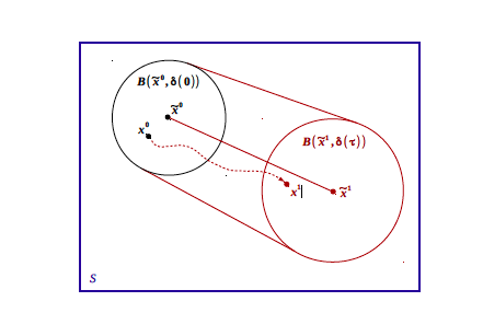
Figure 1: Illustration of Proposition 1

We have:

Theorem 1 (convergence [CF19a]).

Let $y\in{\cal S}$ be a point of $\varepsilon$-representative $z\in{\cal X}$. Let $\pi_{k}^{\varepsilon}$ be the pattern returned by $\mathit{PROC}_{k}^{\varepsilon}(z)$, and $\pi^{\sharp}:=\operatorname*{arg\,min}_{\pi\in U_{k}}\|Y^{\pi}_{y}(k\tau)-y_{f}\|$. Let ${\bf v}_{k}(y):=\|Y_{y}^{\pi^{\sharp}}(k\tau)-y_{\mathit{end}}\|$ be the exact optimal value of $y$. The approximate optimal value of $y$, $\|\tilde{Y}_{y}^{\pi_{k}^{\varepsilon}}(k\tau)-y_{\mathit{end}}\|$, converges to ${\bf v}_{k}(y)$ as $\varepsilon\rightarrow 0$.

Theorem 1 formally justifies the correctness of our method of optimal control synthesis by saying that the approximate optimal values computed by our method converge to the exact optimal values when the mesh size tends to $0$.

II-D Extension to systems with perturbation

Let us now show how the method extends to systems with “bounded perturbations”, and assess its robustness. A differential system with “bounded perturbations” is of the form

$$\frac{dy(t)}{dt}=f_{u}\big{(}y(t),w(t)\big{)}\text{,}$$

with $u\in U$, $t\in[0,\tau]$, states $y(t)\in\mathbb{R}^{n}$, and perturbations $w(t)\in{\cal W}\subset\mathbb{R}^{d}$ (${\cal W}$ is compact, i. e., closed and bounded). See, e. g., [SA17].linecolor=blue,backgroundcolor=blue!25,bordercolor=blue]A: ? Any possible perturbation trajectory is thus bounded in ${\cal W}$, and there exists $\omega\in\mathbb{R}_{\geq 0}$ such that $\forall t\in[0,\tau]$, $\|w(t)\|\leq\omega$. Given a perturbation $w\in{\cal W}$, we use $Y_{y_{0},w}^{u}(t)$ to denote the solution of $\frac{dy(t)}{dt}=f_{u}(y(t),w(t))$ for $t\in[0,\tau]$ with $y(0)=y_{0}$. We use $Y_{y_{0},{\bf 0}}^{u}(t)$ (resp. $\tilde{Y}_{y_{0}}^{u}(t)$) to denote the solution (resp. the approximate Euler solution) without perturbations, i. e., when ${\cal W}=0$.

Given a pattern $\pi=u_{k}\cdots u_{1}\in U^{k}$, these notations extend naturally to $t\in[0,k\tau]$ by considering the solutions obtained by applying successive modes $u_{k},\dots,u_{1}$ in a continuous manner. The optimization task is now to find a control pattern $\pi\in U^{k}$ which guarantees that all states in ${\cal S}\subset\mathbb{R}^{n}$ are steered at time $t=k\tau$ as closely as possible to an end state $y_{\mathit{end}}$, despite the perturbation set ${\cal W}$.

We suppose (see [Le ̵+17]) that, for all $u\in U$, there exist constants $\lambda_{u}\in\mathbb{R}$ and $\gamma_{u}\in\mathbb{R}_{\geq 0}$ such that, for all $y_{1},y_{2}\in{\cal T}$ and $w_{1},w_{2}\in{\cal W}$:

$$\langle f_{u}(y_{1},w_{1})-f_{u}(y_{2},w_{2}),y_{1}-y_{2}\rangle\\ \leq\lambda_{u}\|y_{1}-y_{2}\|^{2}+\gamma_{u}\|y_{1}-y_{2}\|\|w_{1}-w_{2}\|$$ (2)

This formula can be seen as a generalization of Eq. 1 (see Section II). Recall that $\lambda_{u}$ has to be computed in the absence of perturbation (${\cal W}=0$). The additional constant $\gamma_{u}$ is used for taking into account the perturbation $w$. Given $\lambda_{u}$, the constant $\gamma_{u}$ can be computed itself using a nonlinear optimization solver (e. g., CPLEX [IBM09]). Instead of computing them globally for ${\cal T}$, it is advantageous to compute $\lambda_{u}$ and $\gamma_{u}$ locally depending on the subregion of ${\cal T}$ occupied by the system state during a considered interval of time $\Delta t$. Note that the notion of contraction (often used in the literature [MS13, AS14]) corresponds to the case where $\lambda_{u}$ is negative on the whole space set of interest. (Here, $\lambda_{u}$ can be positive, at least locally, see Remark 2.)

We now give a version of Proposition 1 with bounded perturbation $w(\cdot)\in{\cal W}$, originally proved in [Le ̵+17].

Proposition 2 ([Le ̵+17]).

Consider a sampled switched system with bounded perturbation of the form $\{\frac{dy(t)}{dt}=f_{u}(y(t),w(t))\}_{u\in U}$ satisfying Eq. 2.

Consider a point $y_{0}\in{\cal S}$ of $\varepsilon$-representative $z_{0}\in{\cal X}$. We have, for all $u\in U$, $t\in[0,\tau]$ and $w(t)$ with $\|w(t)\|\leq\omega$:

$$\|Y^{u}_{y_{0},w}(t)-\tilde{Y}^{u}_{z_{0}}(t)\|\leq\delta^{u}_{\varepsilon,{\cal W}}(t)$$

with

• if $\lambda_{u}<0$,

  $$\delta^{u}_{\varepsilon,{\cal W}}(t)=\left(\frac{C_{u}^{2}}{-\lambda_{u}^{4}}\left(-\lambda_{u}^{2}t^{2}-2\lambda_{u}t+2e^{\lambda_{u}t}-2\right)\right.\\ +\left.\frac{1}{\lambda_{u}^{2}}\left(\frac{2C_{u}\gamma_{u}\omega}{-\lambda_{u}}\left(-\lambda_{u}t+e^{\lambda_{u}t}-1\right)\right.\right.\\ +\left.\left.\lambda_{u}\left(\frac{\gamma_{u}^{2}\omega^{2}}{-\lambda_{u}}(e^{\lambda_{u}t}-1)+\lambda_{u}\varepsilon^{2}e^{\lambda_{u}t}\right)\right)\right)^{1/2}$$ (3)

• if $\lambda_{u}>0$,

  $$\delta^{u}_{\varepsilon,{\cal W}}(t)=\frac{1}{(3\lambda_{u})^{3/2}}\left(\frac{C_{u}^{2}}{\lambda_{u}}\left(-9\lambda_{u}^{2}t^{2}-6\lambda_{u}t+2e^{3\lambda_{u}t}\right.\right.\\ \left.-2\right)+\left.3\lambda_{u}\left(\frac{2C_{u}\gamma_{u}\omega}{\lambda_{u}}\left(-3\lambda_{u}t+e^{3\lambda_{u}t}-1\right)\right.\right.\\ +\left.\left.3\lambda_{u}\left(\frac{\gamma_{u}^{2}\omega^{2}}{\lambda_{u}}(e^{3\lambda_{u}t}-1)+3\lambda_{u}\varepsilon^{2}e^{3\lambda_{u}t}\right)\right)\right)^{1/2}$$ (4)

• if $\lambda_{u}=0$,

  $$\delta^{u}_{\varepsilon,{\cal W}}(t)=\left({C_{u}^{2}}\left(-t^{2}-2t+2e^{t}-2\right)\right.\\ +\left.\left({2C_{u}\gamma_{u}\omega}\left(-t+e^{t}-1\right)\right.\right.\\ +\left.\left.\left({\gamma_{u}^{2}\omega^{2}}(e^{t}-1)+\varepsilon^{2}e^{t}\right)\right)\right)^{1/2}$$ (5)

Let ${\cal B}^{u}_{{\cal W}}(t)\equiv B(\tilde{Y}^{u}_{z_{0}}(t),\delta^{u}_{\varepsilon,{\cal W}}(t))$. Proposition 2 expresses that, for $t\in[0,\tau]$, the tube ${\cal B}^{u}_{{\cal W}}(t)$ contains all the solutions $Y^{u}_{y_{0},w}(t)$ with $\|y_{0}-z_{0}\|\leq\varepsilon$ and $w\in{\cal W}$, and is therefore robustely (positive) invariant. The function $\delta^{u}_{{\cal W}}:[0,\tau]\rightarrow{\mathbb{R}}^{n}$ extends continuously to $\delta^{\pi}_{\varepsilon,{\cal W}}:[0,k\tau]\rightarrow{\mathbb{R}}^{n}$ for a sequence $\pi$ of $k$ modes, and the robust invariance property now holds for $t\in[0,k\tau]$. The function extends further continuously to $\delta^{\pi^{*}}_{\varepsilon,{\cal W}}(\cdot)$, when considering the iterated application of sequence $\pi$, and robust invariance property now holds for all $t\geq 0$. Under the iterated application of $\pi$, we denote by $Y_{y_{0},w}^{\pi^{*}}(t)$ the exact solution at time $t$, of the system with perturbation $w\in{\cal W}$ and initial condition $y_{0}$. Likewise, we denote by $\tilde{Y}^{\pi^{*}}_{z_{0}}(t)$ (or sometimes just $\tilde{Y}(t)$) the approximate Euler solution at time $t$, of the system without perturbation, with initial condition $z_{0}$.

Remark 2.

Let us give an algorithm to compute local values of $\lambda_{u}$ (to simplify, we assume that $\lambda_{u}$ is independent of $u$). Given an initial ball $B_{0}$ with radius $d_{0}:=\varepsilon$, we calculate the local value $\lambda^{1}$ of $\lambda_{u}$ and the “successor” ball $B_{1}$ of $B_{0}$ at $t=\Delta t$ as follows:

1. Select a candidate ${\cal T}_{1}$ for a convex zone including $B_{0}$ and calculate the contraction rate $-\lambda^{1}$ on ${\cal T}_{1}$.

2. Calculate $B_{1}={\cal B}_{{\cal W}}(\Delta t)$ and $B^{\prime}_{1}={\cal B}_{{\cal W}}(2\Delta t)$ using the function $\delta_{d_{0},{\cal W}}$ associated with $\lambda^{1}$.

3. Check that $B_{1}$ and $B^{\prime}_{1}$ are included in ${\cal T}_{1}$. If yes, $B_{1}$ is indeed the successor ball (of radius $d_{1}=\delta_{d_{0},{\cal W}}(\Delta t)$) of $B_{0}$; if not, go to step 1.

We can repeat the process by taking $B_{1}$ as a new initial ball, select a candidate zone ${\cal T}_{2}$ of rate $-\lambda^{2}$, calculate a ball $B_{2}$ of radius $d_{2}=\delta_{d_{1},{\cal W}}(\Delta t)$ using $\lambda^{2}$, and so on iteratively.

In the following we assume that the bound $\omega$ of the perturbation ${\cal W}$ is large enough so that, for all $\varepsilon\geq 0$ and all local rate of contraction $-\lambda$:

$(H)\ \ \ \ \ \delta_{\varepsilon,{\cal W}}(\Delta t)\geq\varepsilon e^{\lambda\Delta t}$.

III Application to Guaranteed Robustness

We suppose that a control sequence $\pi$ has been generated by $\mathit{PROC}_{k}^{\varepsilon}$ for solving the finite-horizon optimal control problem for the unperturbed system ($w=0$, $T=k\tau=K\Delta t$). We now give a simple condition on the system with perturbation ${\cal W}$ under $\pi^{*}$ which guarantees the existence of a stable LC ${\cal L}$ for the unperturbed system, as well as the boundedness of the solutions of the perturbed system. Let us consider the tube ${\cal B}_{{\cal W}}(t)\equiv B(\tilde{Y}^{\pi^{*}}_{z_{0}}(t),\delta^{\pi^{*}}_{\mu,{\cal W}}(t))$ for some $\mu\geq\varepsilon$.

Lemma 1.

Suppose

$$(*)\ \ \ \ {\cal B}_{{\cal W}}\big{(}(i+K)\Delta t\big{)}\subset{\cal B}_{{\cal W}}(i\Delta t),\ \text{ for some }i\geq 0.$$

Then we have:

1. The set ${\cal I}\equiv\{y\in{\cal B}_{{\cal W}}(t)\}_{t\in[i\Delta t,(i+K)\Delta t]}$ is an invariant of the perturbed system, i.e.: if $y_{0}\in{\cal I}$ then $Y^{\pi^{*}}_{y_{0},{\cal W}}(t)\in{\cal I}$ for all $t\geq 0$.

2. $\lambda^{i+1}+\cdots+\lambda^{i+K}<0$, where $-\lambda^{j}$ ($j=i+1,\dots,i+K$) is the local rate of contraction for the region $\{y\in{\cal B}_{{\cal W}}(t)\}_{t\in[(j-1)\Delta t,j\Delta t]}$.

This implies that the distance between two solutions of the unperturbed system starting at ${\cal I}$ decreases exponentially every $T=K\Delta t$ time-steps, and each solution of the unperturbed system starting at ${\cal I}$ converges to an LC ${\cal L}\subset{\cal I}$.

Proof.

(sketch). Item 1 follows easily from $(*)$. Item 2 is proved ad absurdum: Suppose $\lambda^{i+1}+\cdots+\lambda^{i+K}\geq 0$. It follows, using $(H)$: $\delta_{\mu,{\cal W}}((i+K)\Delta t)\geq e^{(\lambda^{i+1}+\dots+\lambda^{i+K})\Delta t}\delta_{\mu,{\cal W}}(i\Delta t)\geq\delta_{\mu,{\cal W}}(i\Delta t)$. This implies that the radius of ${\cal B}_{{\cal W}}((i+K)\Delta t)$ is greater than or equal to the radius of ${\cal B}_{{\cal W}}(i\Delta t)$, which contradicts $(*)$. So $\lambda^{i+1}+\cdots+\lambda^{i+K}<0$. It follows that ${\cal I}$ is a “contraction” region for the unperturbed system, and every solution starting at $y_{0}\in{\cal I}$ converges to an LC ${\cal L}\subset{\cal I}$ (cf. proof of Theorem 2 in [MS13]). ∎

From Lemma 1, it easily follows:

Theorem 2.

Let $y_{0}\in{\cal S}$ be a point of $\varepsilon$-representative $z_{0}\in{\cal X}$ (so $\|y_{0}-z_{0}\|\leq\varepsilon$). Let $T=k\tau=K\Delta t$. Let $\pi\in U^{k}$ be the optimal pattern output by $\mathit{PROC}_{k}^{\varepsilon}(z_{0})$ for the unperturbed system with finite horizon $T$. Let us consider the tube ${\cal B}_{{\cal W}}(t)\equiv B(\tilde{Y}^{\pi^{*}}_{z_{0}}(t),\delta^{\pi^{*}}_{\mu,{\cal W}}(t))$ for some $\mu\geq\varepsilon$. Suppose that the following inclusion condition holds:

$$(*)\ \ \ \ \ {\cal B}_{{\cal W}}\big{(}(i+K)\Delta t\big{)}\subset{\cal B}_{{\cal W}}(i\Delta t)\text{ for some }i\geq 0\text{.}$$

Then:

1. The exact solution $Y_{y_{0},{\bf 0}}^{\pi^{*}}(t)$ of the unperturbed system under control $\pi^{*}$ converges to an LC ${\cal L}\subset{\cal I}$ when $t\rightarrow\infty$.

2. For all $w\in{\cal W}$, the exact solution $Y_{y_{0},w}^{\pi^{*}}(t)$ of the perturbed system always remains inside ${\cal I}$ for $t\geq i\Delta t$.

This reflects the robustness of the perturbed system under $\pi^{*}$.

Remark 3.

In the OPC literature, it is classical to formulate the optimization problem with an explicit periodicity constraint of the form $Y(T)=Y(0)$ (see, e. g., [Gil77, Hou+09]). This is not needed here. Actually, at the end of the first period $t=T$, $Y(t)$ is in general very different from $Y(0)$ with our method (see Example 2).

Implementation

The implementation has been done in Python and corresponds to a program of around 500 lines. The source code is available at lipn.univ-paris13.fr/~jerray/robust/. In the experiments below, the program runs on a 2.80 GHz Intel Core i7-4810MQ CPU with 8 GiB of memory.

Example 2.

Let us consider the system of Example 1 and the initial point $z_{0}\equiv(X(0),S(0),P(0))=(6.52,12.50,22.40)$ Let $\pi$ be the control sequence $\pi$ found by $\mathit{PROC}(z_{0})$ for the process without perturbation for $\tau=1,\Delta t=1/400$ and $T=48$ (i. e., $k=48$, $K=19200$). Here, $\lambda$ is independent of the value of the mode $S_{f}$. The values of $\lambda$ and $\gamma$ are computed locally and vary from $+4.0$ to $-0.1$, and from $0.06$ to $0.12$ respectively. linecolor=orange,backgroundcolor=orange!25,bordercolor=orange]Laurent: LF: CPU time for computing all the points $z$ of ${\cal X}$??? Let us apply the control sequence $\pi$ repeatedly to the process with perturbation: we suppose here that the perturbation is additive and $\|w\|\leq\omega=0.005$. Fig. 2 displays the results of the 4 first applications of $\pi$. In these figures, the red curves represent the Euler approximation $\tilde{Y}(t)$ of the undisturbed solution as a function of time $t$ in the plans $X$, $S$ and $P$. The green curves correspond, in the $X$, $S$ and $P$ plans, to the borders of tube ${\cal B}_{{\cal W}}(t)\equiv B(\tilde{Y}(t),\delta_{{\cal W}}(t))$ with $\tilde{Y}(0)=z_{0}$ and $\delta_{{\cal W}}(0)=\mu=1$. The 10 blue curves correspond to as many random simulations of the system with perturbation, with initial values in $B(z_{0},\mu)$. It can be seen that the blue curves always remain well inside the green tube ${\cal B}_{{\cal W}}(t)$ which overapproximates the set of solutions of the system with perturbation. The values of the coordinates of the center $\tilde{Y}(t)$ and the radius $\delta_{{\cal W}}(t)$ of the green tube ${\cal B}_{{\cal W}}(t)$, at $t=0,T,2T,3T$, are:

$\tilde{Y}(0)=(6.52,12.5,22.4)$, $\delta_{{\cal W}}(0)=1$;

$\tilde{Y}(T)=(6.78068367,12.61279314,23.98459177)$, $\delta_{{\cal W}}(T)=0.35893$;

$\tilde{Y}(2T)=(6.77663937,12.62347387,23.95516391)$, $\delta_{{\cal W}}(2T)=0.2475$;

$\tilde{Y}(3T)=(6.77670354,12.62331389,23.95558776)$, $\delta_{{\cal W}}(3T)=0.24533$.
We have: ${\cal B}_{{\cal W}}(3T)\subset{\cal B}_{{\cal W}}(2T)\subset{\cal B}_{{\cal W}}(T)$ (but ${\cal B}_{{\cal W}}(T)\not\subseteq{\cal B}_{{\cal W}}(0)$). The computation takes 480 seconds of CPU time. It follows by Theorem 2 that the solution of the perturbed system, for $t\geq 2T$ passes periodically by ${\cal B}_{{\cal W}}(2T)=B(\tilde{Y}(2T),0.2475)$, and the solution of the unperturbed system converges to an LC contained in ${\cal I}\equiv\{(X,S,P)\in{\cal B}_{{\cal W}}(t)\}_{t\in[T,2T]}$. This appears clearly on Fig. 2, where simulations of the process with perturbation corresponds to the blue lines, and the process without perturbation to the red line.

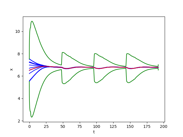
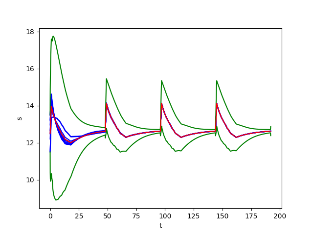
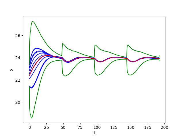
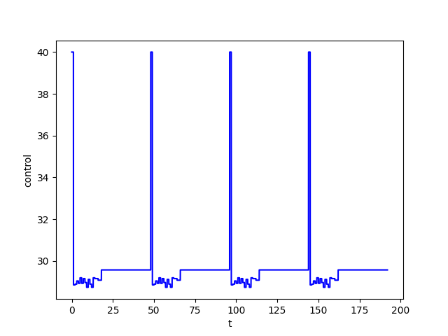
Figure 2: Biochemical process with an additive perturbation $\|w\|\leq 0.005$ over 4 periods ($4T=192$) for $\Delta t=1/400$ and initial condition $(X(0),S(0),P(0))=(6.52,12.5,22.4)$, with, from top to bottom, $X(t)$, $S(t)$, $P(t)$ and control $S_{f}(t)$.

IV Conclusion

We have supposed here that a control sequence $\pi$ has been generated for solving a finite-horizon optimal control problem for the system without perturbation ($w=0$). We have then given a simple condition which guarantees that, under the repeated application $\pi^{*}$ of $\pi$, the system with perturbation ($w\in{\cal W}$) is robust under $\pi^{*}$: the unperturbed system is guaranteed to converge towards an LC ${\cal L}$, and the system perturbed with ${\cal W}$ is guaranteed to stay inside a bounded tube around ${\cal L}$. In contrast with many methods of OPC using elements of the theory of LCs (e. g., [Hou+09, SHD12, Ste+12]), the method does not make use of any notion of monodromy matrix or Lyapunov function. The method uses a simple algorithm to compute local rates of contraction in the framework of Euler’s method (see Remark 2), which may be more accurate than the global rates considered in the literature (see e. g., [AS14, MS13]). The simplicity of application of our method has been illustrated on the example of a bioreactor given in [Hou+09].

As mentioned in Section I, we have treated here a simplified problem of robustness compared to the one dealt with in [Hou+09] (cf. [NB03]). We plan to improve our method in order to take into account the specification of state constraints during the evolution of the system.

References

- [AKR89] Pramod Agrawal, George Koshy and Michael Ramseier “An algorithm for operating a fed-batch fermentor at optimum specific-growth rate” In Biotechnology and Bioengineering 33.1, 1989, pp. 115–125 DOI: 10.1002/bit.260330115
- [AS14] Zahra Aminzare and Eduardo D. Sontag “Contraction methods for nonlinear systems: A brief introduction and some open problems” In CDC, 2014, pp. 3835–3847 DOI: 10.1109/CDC.2014.7039986
- [CF19] Adrien Le Coënt and Laurent Fribourg “Guaranteed Control of Sampled Switched Systems using Semi-Lagrangian Schemes and One-Sided Lipschitz Constants” In CDC Nice, France: IEEE, 2019, pp. 599–604 DOI: 10.1109/CDC40024.2019.9029376
- [CF19a] Adrien Le Coënt and Laurent Fribourg “Guaranteed Optimal Reachability Control of Reaction-Diffusion Equations Using One-Sided Lipschitz Constants and Model Reduction” In WESE 11971, LNCS New York City, NY, USA: Springer, 2019, pp. 181–202 DOI: 10.1007/978-3-030-41131-2˙9
- [DT12] Hongkai Dai and Russ Tedrake “Optimizing robust limit cycles for legged locomotion on unknown terrain” In CDC Maui, HI, USA: IEEE, 2012, pp. 1207–1213 DOI: 10.1109/CDC.2012.6425971
- [FM15] Chuchu Fan and Sayan Mitra “Bounded Verification with On-the-Fly Discrepancy Computation” In ATVA 9364, LNCS Shanghai, China: Springer, 2015, pp. 446–463 DOI: 10.1007/978-3-319-24953-7˙32
- [Gil77] Elmer Gilbert “Optimal Periodic Control: A General Theory of Necessary Conditions” In SIAM Journal on Control and Optimization 15.5, 1977, pp. 717–746
- [Hou+09] Boris Houska, Filip Logist, Jan F.. Impe and Moritz Diehl “Approximate robust optimization of time-periodic stationary states with application to biochemical processes” In CDC Shanghai, China: IEEE, 2009, pp. 6280–6285 DOI: 10.1109/CDC.2009.5400684
- [IBM09] IBM ILOG “User’s Manual for CPLEX” Cplex V12.1 In International Business Machines Corporation 46.53, 2009 URL: ftp://public.dhe.ibm.com/software/websphere/ilog/docs/optimization/cplex/ps_usrmancplex.pdf
- [KSC93] G. Kumar, I… Sastry and M. Chidambaram “Periodic operation of a bioreactor with input multiplicities” In The Canadian Journal of Chemical Engineering 71.5, 1993, pp. 766–770 DOI: 10.1002/cjce.5450710515
- [Le ̵+17] Adrien Le Coënt et al. “Distributed Control Synthesis using Euler’s Method” In RP 247, LNCS London, UK: Springer, 2017, pp. 118–131 DOI: 10.1007/978-3-319-67089-8˙9
- [Le ̵+17a] Adrien Le Coënt, Florian De Vuyst, Ludovic Chamoin and Laurent Fribourg “Control Synthesis of Nonlinear Sampled Switched Systems using Euler’s Method” In SNR 247, EPTCS, 2017, pp. 18–33 DOI: 10.4204/EPTCS.247.2
- [MS13] Ian R. Manchester and Jean-Jacques E. Slotine “Transverse contraction criteria for existence, stability, and robustness of a limit cycle” In CDC Firenze, Italy: IEEE, 2013, pp. 5909–5914 DOI: 10.1109/CDC.2013.6760821
- [NB03] Zoltan K. Nagy and Richard D. Braatz “Worst-case and distributional robustness analysis of finite-time control trajectories for nonlinear distributed parameter systems” In IEEE Transactions on Control Systems Technology 11.5, 2003, pp. 694–704 DOI: 10.1109/TCST.2003.816419
- [Par00] Satish Parulekar “Analysis of forced periodic operations of continuous bioprocesses – Single input variations” In Chemical Engineering Science 55, 2000, pp. 513–533 DOI: 10.1016/S0009-2509(99)00317-6
- [RC08] Lier Ruan and Xiao Chen “Comparison of Several Periodic Operations of a Continuous Fermentation Process” In Biotechnology Progress 12, 2008, pp. 286–288 DOI: 10.1021/bp960006l
- [SA17] Bastian Schürmann and Matthias Althoff “Guaranteeing Constraints of Disturbed Nonlinear Systems Using Set-Based Optimal Control in Generator Space” 20th IFAC World Congress In IFAC-PapersOnLine 50.1, 2017, pp. 11515–11522 DOI: 10.1016/j.ifacol.2017.08.1617
- [SHD12] Julia Sternberg, Boris Houska and Moritz Diehl “A structure exploiting algorithm for approximate robust optimal control with application to power generating kites” In ACC Montréal, QC, Canada: IEEE, 2012, pp. 2250–2255 DOI: 10.1109/ACC.2012.6314896
- [Ste+12] Julia Sternberg, Boris Houska, Sebastien Gros and Moritz Diehl “Approximate Robust Optimal Control of Periodic Systems with Invariants and High-Index Differential Algebraic Systems” In ROCOND Aalborg, Denmark: International Federation of Automatic Control, 2012, pp. 690–695 DOI: 10.3182/20120620-3-DK-2025.00089
- [Thu+18] Thomas George Thuruthel, Egidio Falotico, Mariangela Manti and Cecilia Laschi “Stable Open Loop Control of Soft Robotic Manipulators” In IEEE Robotics and Automation Letters 3.2, 2018, pp. 1292–1298 DOI: 10.1109/LRA.2018.2797241
- [Wan+19] Wenkai Wang, Zhongxi Hou, Shangqiu Shan and Lili Chen “Optimal Periodic Control of Hypersonic Cruise Vehicle: Trajectory Features” In IEEE Access 7, 2019, pp. 3406–3421 DOI: 10.1109/ACCESS.2018.2885597