Fast primal-dual algorithm via dynamical system for a linearly constrained convex optimization problem

Abstract

By time discretization of a second-order primal-dual dynamical system with damping $\alpha/t$ where an inertial construction in the sense of Nesterov is needed only for the primal variable, we propose a fast primal-dual algorithm for a linear equality constrained convex optimization problem. Under a suitable scaling condition, we show that the proposed algorithm enjoys a fast convergence rate for the objective residual and the feasibility violation, and the decay rate can reach $\mathcal{O}(1/k^{\alpha-1})$ at the most. We also study convergence properties of the corresponding primal-dual dynamical system to better understand the acceleration scheme. Finally, we report numerical experiments to demonstrate the effectiveness of the proposed algorithm.

, ,

1 Introduction

Let $\mathbb{R}^{n}$ be an $n$-dimensional Euclidean space with the scalar product $\langle\cdot,\cdot\rangle$ and the corresponding induced norm $\|\cdot\|$. Let $f:\mathbb{R}^{n}\to\mathbb{R}\cup\{+\infty\}$ be a proper, lower semicontinuous and convex function, $A\in\mathbb{R}^{m\times n}$, and $b\in\mathbb{R}^{m}$. Consider the linearly constrained convex optimization problem

$$\min_{x\in\mathbb{R}^{n}}\quad f(x),\quad s.t.\ Ax=b.$$ (1)

The problem (1) is a basic model for many important applications arising in various areas, such as compressive sensing, image processing, global consensus and machine learning problems. See e.g. Candès & Wakin (2008); Boyd et al. (2011); Lin, Li, & Fang (2020); Feijer & Paganini (2010); Zhang et al. (2010); Zhu et al. (2020); Wang et al. (2021).

Denote the KKT point set of the problem (1) by $\Omega$. For any $(x^{*},\lambda^{*})\in\Omega$, we have

$$\begin{cases}-A^{T}\lambda^{*}\in\partial f(x^{*}),\\ Ax^{*}=b,\end{cases}$$ (2)

where

$$\partial f(x)=\{v\in\mathbb{R}^{n}\ |\ f(y)\geq f(x)+\langle v,y-x\rangle,\quad\forall y\in\mathbb{R}^{n}\}.$$

Recall the Lagrangian function of the problem (1),

$$\mathcal{L}(x,\lambda)=f(x)+\langle\lambda,Ax-b\rangle,$$

where $\lambda\in\mathbb{R}^{m}$ is the Lagrange multiplier. From (2) we have

$$\mathcal{L}(x^{*},\lambda)\leq\mathcal{L}(x^{*},\lambda^{*})\leq\mathcal{L}(x,\lambda^{*}),\ \ \forall(x,\lambda)\in\mathbb{R}^{n}\times\mathbb{R}^{m}.$$

Throughout this paper, we always assume $\Omega\neq\emptyset$.

1.1 Literature review

A benchmark algorithm for the problem (1) is the augmented Lagrangian method (ALM)

$$\begin{cases}x_{k+1}\in\mathop{\arg\min}_{x}f(x)+\langle\lambda_{k},Ax-b\rangle+\frac{\sigma}{2}\|Ax-b\|^{2},\\ \lambda_{k+1}=\lambda_{k}+\sigma(Ax_{k+1}-b).\end{cases}$$

ALM plays a fundamentally theoretical and algorithmic role in solving the problem (1). Here, we mention some of nice works concerning fast convergence properties of ALM and its variants. By applying Nesterov’s acceleration technique Nesterov (2003, 1983) to ALM, He & Yuan (2010) developed an accelerated augmented Lagrangian method (AALM) for the problem (1) and proved that AALM enjoys the $\mathcal{O}(1/k^{2})$ convergence rate when $f$ is differentiable. When $f$ is nondifferentiable, the $\mathcal{O}(1/k^{2})$ convergence rate of AALM was established in Kang et al. (2013). Kang, Kang, & Jung (2015) further proposed an inexact version of AALM and demonstrated the $\mathcal{O}(1/k^{2})$ convergence rate under the strong convexity assumption of $f$. Huang, Ma, & Goldfarb (2013) considered an accelerated linearized Bregman method for solving the basis pursuit and related sparse optimization problems, and proved that it owns the $\mathcal{O}(1/k^{2})$ convergence rate. It is worth noting that the convergence rate analysis of the accelerated algorithms mentioned above was done for the Lagrangian residual $\mathcal{L}(x^{*},\lambda^{*})-\mathcal{L}(x_{k},\lambda_{k})$. Recently, Xu (2017) presented an accelerated ALM for solving the problem (1). By adapting parameters during the iterations, they proved that the objective residual and the feasibility violation both enjoy the $\mathcal{O}(1/k^{2})$ convergence rate. By applying Nesterov’s technique, He, Hu, & Fang (2022) proposed two accelerated primal-dual algorithms, which enjoy the $\mathcal{O}(1/k^{2})$ convergence rate of the objective residual and the feasibility violation. In terms of scaling coefficients, He, Hu, & Fang (2021b); Luo (2022); Yan & He (2020) proposed accelerated ALM algorithms in different ways, and obtained the fast convergence rates related to the scaling coefficients. By time discretization of a second-order dynamical system, Luo (2021b) proposed new accelerated primal-dual methods, and derived the $\mathcal{O}(1/k^{2})$ convergence rate for the primal-dual gap, the feasibility violation and the objective residual under the assumption that the objective function is strongly convex. In the case that $f$ has a Lipschitz continuous gradient, Boţ, Csetnek, & Nguyen (2021) proposed fast ALM algorithms by time discretization of the dynamical system in Boţ & Nguyen (2021). They proved the $\mathcal{O}(1/k^{2})$ convergence rate of the primal-dual gap, the feasibility measure and the objective residual, and also showed the convergence of the sequence of iterations. From the variational perspective, Fazlyab et al. (2017) proposed accelerated higher-order gradient methods by discretization of a second-order dual dynamical system and exhibited the $\mathcal{O}(1/k^{p})$ converges rate of the dual residual and the $\mathcal{O}(1/k^{p/2})$ rate of the feasibility violation under the assumption that the objective function is strong convex and has a $(p-1)$–th Lipschitz gradient.

1.2 Fast primal-dual algorithm via dynamical system

Dynamical system methods have been recognized as efficient tools for solving optimization problems in the literature. Dynamical systems can not only give more insights into the existing numerical methods for optimization problems but also lead to other possible numerical algorithms by time discretization, see e.g. Chen & Luo (2021); Liang & Yin (2019); Jordan (2018); Su, Boyd, & Candès (2016); Wilson, Recht, & Jordan (2021); Attouch et al. (2018); Luo (2021a); Kia, Cortés, & Martínez (2015). In this paper, we will propose a fast primal-dual algorithm via time discretization of the following primal-dual dynamical system

$$\begin{cases}\ddot{x}(t)+\frac{\alpha}{t}\dot{x}(t)&=-\beta(t)(\nabla f(x(t))+A^{T}\lambda(t))+\epsilon(t),\\ \dot{\lambda}(t)&=t\beta(t)(A(x(t)+\frac{t}{\alpha-1}\dot{x}(t))-b),\end{cases}$$ (3)

where $t\geq t_{0}>0$, $\alpha/t$ with $\alpha>1$ is a damping coefficient, $\beta:[t_{0},+\infty)\to(0,+\infty)$ is a scaling coefficient, and $\epsilon:[t_{0},+\infty)\to\mathbb{R}^{n}$ is a perturbation coefficient.

Su, Boyd, & Candès (2016) showed that the damping ${\alpha}/{t}$ with $\alpha=3$ in inertial dynamical systems for unconstrained convex optimization problems can be understood as the continuous limit of Nesterov’s accelerated technique Nesterov (1983). By considering the damping ${\alpha}/{t}$ with $\alpha\geq 3$ and the scaling $\beta(t)$, Attouch, Chbani, & Riahi (2019); Wibisono, Wilson, & Jordan (2016) obtained the $\mathcal{O}(1/t^{2}\beta(t))$ convergence rate of dynamical systems for solving unconstrained convex optimization problems and also obtained the rate-matching inertial algorithms by different time discretization schemes. Recently, some researchers extended the dynamical systems in Su, Boyd, & Candès (2016); Attouch, Chbani, & Riahi (2019); Wibisono, Wilson, & Jordan (2016) to inertial primal-dual dynamical systems for solving the problem (1). See e.g. He, Hu, & Fang (2021a); Attouch et al. (2022); Zeng, Lei, & Chen (2022); Boţ & Nguyen (2021). Very recently, by time discretization of the inertial dynamical system, Boţ, Csetnek, & Nguyen (2021) proposed new ALM algorithms with $\mathcal{O}(1/k^{2})$ convergence rate. It is worth mentioning that for the dynamical systems mentioned above, inertial constructions are needed for both the primal variable and the dual variable. As a comparison, the inertial term is considered in the dynamical system (3) only for the primal variable.

In the next, by time discretization of (3), we will propose an accelerated primal-dual algorithm. Rewrite (3) as

$$\begin{cases}y(t)&=x(t)+\frac{t}{\alpha-1}\dot{x}(t),\\ \frac{\alpha-1}{t}\dot{y}(t)&=-\beta(t)(\nabla f(x(t))+A^{T}\lambda(t))+\epsilon(t),\\ \dot{\lambda}(t)&=t\beta(t)(Ay(t)-b).\end{cases}$$ (4)

Set $t_{k}=k,x_{k}=x(t_{k}),\ y_{k}=y(t_{k}),\ \lambda_{k}=\lambda(t_{k}),\ \beta_{k}=\beta(t_{k})$, $\epsilon_{k}=\epsilon(t_{k})$. Take the following discretization scheme of (4) with a nondifferentiable function $f$

$$y_{k}=x_{k}+\frac{k-\theta}{\alpha-1}(x_{k}-x_{k-1}),$$ (5a)

$$\frac{\alpha-1}{k}(y_{k+1}-y_{k})$$

$$\qquad\quad\in-\beta_{k}(\partial f(x_{k+1})+A^{T}\lambda_{k+1})+\epsilon_{k},$$ (5b)

$$\lambda_{k+1}-\lambda_{k}=k\beta_{k}(Ay_{k+1}-b),$$ (5c)

where $\theta\in\mathbb{R}$. Substitute (5a) and (5c) into (5b) to obtain

$$\frac{k+\alpha-\theta}{k}\left(x_{k+1}-\left(x_{k}+\frac{k-\theta}{k+\alpha-\theta}(x_{k}-x_{k-1})\right)\right)$$

$$\ \in-\beta_{k}(\partial f(x_{k+1})+A^{T}\lambda_{k})+\epsilon_{k}$$ (6)

$$\quad-k\beta_{k}^{2}A^{T}\left(A\left(x_{k+1}+\frac{k+1-\theta}{\alpha-1}(x_{k+1}-x_{k})\right)-b\right).$$

Then, we can write (5) as Algorithm 1 for solving problem (1).

Algorithm 1 Fast primal-dual algorithm

Initialization: Choose $x_{0}\in\mathbb{R}^{n},\ \lambda_{0}\in\mathbb{R}^{m}$, $\alpha>1$, $\theta\in\mathbb{R}$. Set $x_{1}=x_{0},\ \lambda_{1}=\lambda_{0}$.
For $k=1,2,\cdots$do

Step 1: Compute $\bar{x}_{k}=x_{k}+\frac{k-\theta}{k+\alpha-\theta}(x_{k}-x_{k-1})$.

Step 2: Choose $\beta_{k}>0$. Set

$$\vartheta_{k}=\frac{k(k+\alpha-\theta)\beta_{k}}{\alpha-1},$$

$$\eta_{k}=\frac{k+1-\theta}{k+\alpha-\theta}Ax_{k}+\frac{\alpha-1}{k+\alpha-\theta}b.$$

Update the primal variable

$$\qquad x_{k+1} = \mathop{\arg\min}_{x\in\mathbb{R}^{n}}\ \{f(x)+\frac{k+\alpha-\theta}{2k\beta_{k}}\|x-\bar{x}_{k}\|^{2}$$

$$+\frac{\vartheta_{k}}{2}\|Ax-\eta_{k}\|^{2}+\langle A^{T}{\lambda}_{k}-\frac{\epsilon_{k}}{\beta_{k}},x\rangle\}.$$

Step 3: Compute

$$y_{k+1}=x_{k+1}+\frac{k+1-\theta}{\alpha-1}(x_{k+1}-x_{k}).$$

Update the dual variable

$$\quad\lambda_{k+1}=\lambda_{k}+k\beta_{k}(Ay_{k+1}-b).$$

If A stopping condition is satisfied then

Return $(x_{k+1},\lambda_{k+1})$

end
end

The perturbation $\epsilon(t)$ in (3) can be interpreted as a kind of disturbance, and here we adopt the terminology “perturbation” used by Attouch et al. (2018); He, Hu, & Fang (2021a). In Step 2 of Algorithm 1, the perturbation $\epsilon_{k}$ means

$$\qquad x_{k+1} \approx \mathop{\arg\min}_{x\in\mathbb{R}^{n}}\ \{f(x)+\frac{k+\alpha-\theta}{2k\beta_{k}}\|x-\bar{x}_{k}\|^{2}$$

$$+\frac{\vartheta_{k}}{2}\|Ax-\eta_{k}\|^{2}+\langle A^{T}{\lambda}_{k},x\rangle\}.$$

The $x$-subproblem in Step 2 of Algorithm 1 has a special splitting structure and it can be efficiently solved by some classical splitting methods such as the proximal gradient method and its accelerated version FISTA (see e.g. Beck & Teboulle (2009); Lin, Li, & Fang (2020)).

In this paper, by constructing a discrete energy sequence and a continuous energy function, we show fast convergence properties of Algorithm 1 and the dynamical system (3). Our main contributions are summarized as follows:

(a): The discrete level: By time discretization of the dynamical system (3) with damping $\alpha/t$ and scaling $\beta(t)$, we obtain Algorithm 1. Under a suitable scaling condition, we obtain the $\mathcal{O}(1/k^{2}\beta_{k})$ convergence rate of the objective residual and the feasibility violation, which can reach $\mathcal{O}(1/k^{\alpha-1})$ decay rate at the most. We extend (Attouch, Chbani, & Riahi, 2019, Theorem 3.1 and Theorem 7.1) from the unconstrained optimization problem to the linearly constrained convex optimization problem (1). Compared with the accelerated gradient methods in Boţ, Csetnek, & Nguyen (2021) where $f$ is convex and has a Lipschitz gradient, and Fazlyab et al. (2017) where $f$ is strongly convex, Algorithm 1 requires neither strong convexity nor Lipschitz gradient assumption on $f$. In the case $\alpha>3$, we show that Algorithm 1 can achieve a rate faster than $\mathcal{O}(1/k^{2})$ under a suitable scaling condition.

(b) The continuous level: For a better understanding of the acceleration scheme of Algorithm 1, we consider the primal-dual dynamical system (3) and show that it enjoys convergence properties matching to that of Algorithm 1. To the best of our knowledge, the dynamical system (3) is the first Nesterov’s inertial one involving inertial term only for the primal variable for the linearly constrained optimization problem. Our dynamical system (3) extends the dynamical system in He, Hu, & Fang (2021b), which is linked to Polyak’ heavy ball scheme, from the constant viscous damping to the vanishing damping ${\alpha}/{t}$. Compared with a recent work by Attouch et al. (2022), where a general ADMM dynamical system involving inertial terms both for the primal and dual variables was considered for a separable linearly constrained optimization problem, by a new result (Lemma 6), we will prove that the convergence results of the dynamical system (3) are better than the one in (Attouch et al., 2022, Theorem 1). By Lemma 6, we also can improve the convergence of the objective residual and the feasibility violation in (Attouch et al., 2022, Theorem 1) from $\mathcal{O}(1/t^{{1}/{2\alpha_{0}}})$ to $\mathcal{O}(1/t^{{1}/{\alpha_{0}}})$. In the case $\beta(t)\equiv\beta>0$, the dynamical system (3) enjoys the same convergence rate as the dynamical systems in Boţ & Nguyen (2021); Zeng, Lei, & Chen (2022), which involve inertial terms both for the primal and dual variables.

1.3 Organization

The paper is organized as follows: In Section 2, we show the fast convergence properties of Algorithm 1 under a suitable scaling condition. Section 3 is devoted to the study of convergence properties of the inertial primal-dual dynamical system (3). The numerical experiments are given in Section 4. Finally, we end the paper with a conclusion.

2 Fast convergence analysis of Algorithm 1

Before presenting the convergence analysis, we first show that Algorithm 1 is equivalent to the time discretization scheme (5).

Proposition 1.

Algorithm 1 is equivalent to the time discretization scheme (5).

By using the optimality criterion, from Step 2 of Algorithm 1, we get

$$0 \in \partial f(x_{k+1})+\frac{k+\alpha-\theta}{k\beta_{k}}(x_{k+1}-\bar{x}_{k})$$

$$+A^{T}(\vartheta_{k}(Ax_{k+1}-\eta_{k})+{\lambda}_{k})-\frac{\epsilon_{k}}{\beta_{k}},$$

which can be rewritten as

$$\frac{k+\alpha-\theta}{k}(x_{k+1}-\bar{x}_{k})\in-\beta_{k}(\partial f(x_{k+1})$$

$$\qquad+A^{T}(\vartheta_{k}(Ax_{k+1}-\eta_{k})+{\lambda}_{k}))+\epsilon_{k}.$$ (7)

It follows from Step 2 and Step 3 of Algorithm 1 that

$$\vartheta_{k}(Ax_{k+1}-\eta_{k})=\frac{k(k+\alpha-\theta)\beta_{k}}{\alpha-1}Ax_{k+1}$$

$$\qquad-\frac{k(k+1-\theta)\beta_{k}}{\alpha-1}Ax_{k}-k\beta_{k}b$$ (8)

$$\quad=k\beta_{k}(A(x_{k+1}+\frac{k+1-\theta}{\alpha-1}(x_{k+1}-x_{k}))-b).$$

As a consequence of (2), (2) and Step 1, the equation (1.2) holds. By comparing Algorithm 1 and (5), the sequence $\{(x_{k},y_{k},\lambda_{k})\}_{k\geq 1}$ generated by Algorithm 1 satisfies (5). Since the calculation process from above is reversible, from (5), we also can obtain Algorithm 1.

2.1 Convergence analysis for fast primal-dual algorithm

Before discussing the convergence properties of Algorithm 1, we first recall the equality

$$\frac{1}{2}\|x\|^{2}-\frac{1}{2}\|y\|^{2}=\langle x,x-y\rangle-\frac{1}{2}\|x-y\|^{2}$$ (9)

for any $x,y,z\in\mathbb{R}^{n}$, which will be used repeatedly.

Lemma 1.

Let $\{(x_{k},y_{k},\lambda_{k})\}_{k\geq 1}$ be the sequence generated by Algorithm 1 and $(x^{*},\lambda^{*})\in\Omega$. Define the energy sequence

$$\mathcal{E}^{\epsilon}_{k}=\mathcal{E}_{k}-\sum^{k}_{j=1}\langle(\alpha-1)(y_{j}-x^{*}),(j-1)\epsilon_{j-1}\rangle$$ (10)

with

$$\mathcal{E}_{k} = k(k+1-\theta)\beta_{k}(\mathcal{L}(x_{k},\lambda^{*})-\mathcal{L}(x^{*},\lambda^{*}))$$ (11)

$$+\frac{1}{2}\|(\alpha-1)(y_{k}-x^{*})\|^{2}+\frac{\alpha-1}{2}\|\lambda_{k}-\lambda^{*}\|^{2}.$$

Then, for any $k\geq\max\{1,\theta-1\}$:

$$\mathcal{E}^{\epsilon}_{k+1}-\mathcal{E}^{\epsilon}_{k}$$

$$\qquad\leq((k+1)(k+2-\theta)\beta_{k+1}-k\left(k+\alpha-\theta)\beta_{k}\right)$$

$$\quad\qquad\cdot(\mathcal{L}(x_{k+1},\lambda^{*})-\mathcal{L}(x^{*},\lambda^{*})).$$ (12)

By the definition of $\mathcal{L}$, we have

$$\partial_{x}\mathcal{L}(x,\lambda)=\partial f(x)+A^{T}\lambda.$$

This together with (5b) implies

$$(\alpha-1)(y_{k+1}-y_{k})$$

$$\in k(-\beta_{k}(\partial f(x_{k+1})+A^{T}\lambda_{k+1})+\epsilon_{k})$$

$$=k(-\beta_{k}(\partial f(x_{k+1})+A^{T}\lambda^{*})-\beta_{k}A^{T}(\lambda_{k+1}-\lambda^{*})+\epsilon_{k})$$

$$=-k\beta_{k}\partial_{x}\mathcal{L}(x_{k+1},\lambda^{*})-k\beta_{k}A^{T}(\lambda_{k+1}-\lambda^{*})+k\epsilon_{k}.$$

Denote

$$\quad\xi_{k} := -\frac{\alpha-1}{k\beta_{k}}(y_{k+1}-y_{k})-A^{T}(\lambda_{k+1}-\lambda^{*})+\frac{\epsilon_{k}}{\beta_{k}}$$ (13)

$$\in \partial_{x}\mathcal{L}(x_{k+1},\lambda^{*}).$$

Combining (9), (13) and $\alpha>1$, we have

$$\frac{1}{2}\|(\alpha-1)(y_{k+1}-x^{*})\|^{2}-\frac{1}{2}\|(\alpha-1)(y_{k}-x^{*})\|^{2}$$

$$=\langle(\alpha-1)(y_{k+1}-x^{*}),(\alpha-1)(y_{k+1}-y_{k})\rangle$$

$$\quad-\frac{(\alpha-1)^{2}}{2}\|y_{k+1}-y_{k}\|^{2}$$ (14)

$$\leq-k\beta_{k}\langle(\alpha-1)(y_{k+1}-x^{*}),\xi_{k}\rangle$$

$$\quad-k\beta_{k}\langle(\alpha-1)(y_{k+1}-x^{*}),A^{T}(\lambda_{k+1}-\lambda^{*})\rangle$$

$$\quad+\langle(\alpha-1)(y_{k+1}-x^{*}),k\epsilon_{k}\rangle.$$

From assumption we have $k+1-\theta\geq 0$ and $\alpha>1$. By (13) and Step 3, we get

$$\langle(\alpha-1)(y_{k+1}-x^{*}),\xi_{k}\rangle$$

$$\ =(\alpha-1)\langle x_{k+1}-x^{*},\xi_{k}\rangle+(k+1-\theta)\langle x_{k+1}-x_{k},\xi_{k}\rangle$$

$$\ \geq(\alpha-1)(\mathcal{L}(x_{k+1},\lambda^{*})-\mathcal{L}(x^{*},\lambda^{*}))$$ (15)

$$\quad+(k+1-\theta)(\mathcal{L}(x_{k+1},\lambda^{*})-\mathcal{L}(x_{k},\lambda^{*})),$$

where the inequality follows from the convexity of $\mathcal{L}(\cdot,\lambda^{*})$. By Step 3, $Ax^{*}=b$, and (9), we get

$$\frac{1}{2}\|\lambda_{k+1}-\lambda^{*}\|^{2}-\frac{1}{2}\|\lambda_{k}-\lambda^{*}\|^{2}$$

$$\quad=\langle\lambda_{k+1}-\lambda^{*},\lambda_{k+1}-\lambda_{k}\rangle-\frac{1}{2}\|\lambda_{k+1}-\lambda_{k}\|^{2}$$ (16)

$$\quad\leq\langle\lambda_{k+1}-\lambda^{*},k\beta_{k}A(y_{k+1}-x^{*})\rangle.$$

It follows from (10) and (11) that

$$\mathcal{E}^{\epsilon}_{k+1}-\mathcal{E}^{\epsilon}_{k}=\mathcal{E}_{k+1}-\mathcal{E}_{k}-\langle(\alpha-1)(y_{k+1}-x^{*}),k\epsilon_{k}\rangle$$

$$\ \leq((k+1)(k+2-\theta)\beta_{k+1}-k(k+\alpha-\theta)\beta_{k})$$

$$\quad\cdot(\mathcal{L}(x_{k+1},\lambda^{*})-\mathcal{L}(x^{*},\lambda^{*}))$$

$$\quad-k\beta_{k}\langle(\alpha-1)(y_{k+1}-x^{*}),A^{T}(\lambda_{k+1}-\lambda^{*})\rangle$$

$$\quad+\frac{\alpha-1}{2}(\|\lambda_{k+1}-\lambda^{*}\|^{2}-\|\lambda_{k}-\lambda^{*}\|^{2})$$

$$\ \leq((k+1)(k+2-\theta)\beta_{k+1}-k(k+\alpha-\theta)\beta_{k})$$

$$\quad\cdot(\mathcal{L}(x_{k+1},\lambda^{*})-\mathcal{L}(x^{*},\lambda^{*})),$$

where the first inequality follows from (2.1) and (2.1), and the last inequality follows from (2.1). This yields the desired result.

To derive the fast convergence rates, we need the following scaling condition: there exist $k_{1}\geq\max\{2,\theta\}$ such that

$$\beta_{k+1}\leq\frac{k(k+\alpha-\theta)}{(k+1)(k+2-\theta)}\beta_{k},\quad\forall k\geq k_{1}-1.$$ (17)

Now, we start to discuss the fast convergence properties of Algorithm 1 by the Lyapunov analysis approach.

Theorem 1.

Let $\{(x_{k},y_{k},\lambda_{k})\}_{k\geq 1}$ be the sequence generated by Algorithm 1 and $(x^{*},\lambda^{*})\in\Omega$. Assume that the condition (17) holds and

$$\sum^{+\infty}_{k=1}k\|\epsilon_{k}\|<+\infty,\quad\lim_{k\to+\infty}k^{2}\beta_{k}=+\infty.$$

Then, the sequence $\{(y_{k},\lambda_{k})\}_{k\geq k_{1}}$ is bounded,

$$\|Ax_{k}-b\|=\mathcal{O}\left(\frac{1}{k^{2}\beta_{k}}\right),$$

and

$$|f(x_{k})-f(x^{*})|=\mathcal{O}\left(\frac{1}{k^{2}\beta_{k}}\right).$$

From assumptions, we can get $\mathcal{L}(x_{k+1},\lambda^{*})-\mathcal{L}(x^{*},\lambda^{*})\geq 0$ and $(k+1)(k+2-\theta)\beta_{k+1}-k(k+\alpha-\theta)\beta_{k}\leq 0$ for any $k\geq k_{1}$. Then, for any $k\geq k_{1}$, $\mathcal{E}_{k}\geq 0$, and from Lemma 1 we have

$$\mathcal{E}^{\epsilon}_{k}\leq\mathcal{E}^{\epsilon}_{k_{1}},\qquad\forall k\geq k_{1}.$$

By (10) and (11), we have

$$\frac{1}{2}\|(\alpha-1)(y_{k}-x^{*})\|^{2}\leq\mathcal{E}_{k}$$

$$\qquad=\mathcal{E}^{\epsilon}_{k}+\sum^{k}_{j=1}\langle(\alpha-1)(y_{j}-x^{*}),(j-1)\epsilon_{j-1}\rangle$$

$$\qquad\leq\mathcal{E}^{\epsilon}_{k_{1}}+\sum^{k}_{j=1}\langle(\alpha-1)(y_{j}-x^{*}),(j-1)\epsilon_{j-1}\rangle$$ (18)

$$\qquad=\mathcal{E}_{k_{1}}+\sum^{k}_{j=k_{1}+1}\langle(\alpha-1)(y_{j}-x^{*}),(j-1)\epsilon_{j-1}\rangle$$

$$\qquad\leq\mathcal{E}_{k_{1}}+\sum^{k}_{j=k_{1}}(j-1)\|(\alpha-1)(y_{j}-x^{*})\|\cdot\|\epsilon_{j-1}\|$$

for any $k\geq k_{1}$. Note that $\sum^{+\infty}_{k=1}k\|\epsilon_{k}\|<+\infty$. Applying Lemma 2 with $a_{k}=\|(\alpha-1)(y_{k+k_{1}-1}-x^{*})\|$, we get

$$\sup_{k\geq k_{1}}\|(\alpha-1)(y_{k}-x^{*})\|=\sup_{k\geq 1}a_{k}<+\infty.$$

This together with (2.1) yields

$$\sup_{k\geq k_{1}}\mathcal{E}_{k}\leq\mathcal{E}_{k_{1}}+\sup_{k\geq k_{1}}\|(\alpha-1)(y_{k}-x^{*})\|\cdot\sum^{+\infty}_{j=1}j\|\epsilon_{j}\|<+\infty.$$

Thus, the energy sequence $\{\mathcal{E}_{k}\}_{k\geq k_{1}}$ is bounded. By (11), $\{\|y_{k}-x^{*}\|\}_{k\geq k_{1}}$ and $\{\|\lambda_{k}-\lambda^{*}\|\}_{k\geq k_{1}}$ are bounded and

$$\sup_{k\geq k_{1}}k(k+1-\theta)\beta_{k}(\mathcal{L}(x_{k},\lambda^{*})-\mathcal{L}(x^{*},\lambda^{*}))<+\infty.$$ (19)

As a result, the sequence $\{(y_{k},\lambda_{k})\}_{k\geq k_{1}}$ is bounded. From (19) we obtain

$$\mathcal{L}(x_{k},\lambda^{*})-\mathcal{L}(x^{*},\lambda^{*})=\mathcal{O}\left({1}/{k^{2}\beta_{k}}\right).$$ (20)

For notation simplicity, denote

$$g_{k}:=\frac{(k+\alpha-\theta-1)(k-1)\beta_{k-1}}{\alpha-1}(Ax_{k}-b).$$ (21)

It follows from Step 3 that

$$\lambda_{k+1}-\lambda_{k_{1}}=\sum^{k}_{j=k_{1}}(\lambda_{j+1}-\lambda_{j})$$

$$=\sum^{k}_{j=k_{1}}j\beta_{j}(Ay_{j+1}-b)$$ (22)

$$=\sum^{k}_{j=k_{1}}j\beta_{j}\left((Ax_{j+1}-b)+\frac{j+1-\theta}{\alpha-1}A(x_{j+1}-x_{j})\right)$$

$$=\sum^{k}_{j=k_{1}}\left(g_{j+1}-\frac{(j+1-\theta)j\beta_{j}}{(j+\alpha-\theta-1)(j-1)\beta_{j-1}}g_{j}\right)$$

for any $k\geq k_{1}$. Let

$$a_{k}=1-\frac{(k+1-\theta)k\beta_{k}}{(k+\alpha-\theta-1)(k-1)\beta_{k-1}},\quad\forall k\geq k_{1}.$$

From (2.1), we have

$$\lambda_{k+1}-\lambda_{k_{1}} = \sum^{k}_{j=k_{1}}(g_{j+1}-g_{j})+\sum^{k}_{j=k_{1}}a_{j}g_{j}$$

$$= g_{k+1}-g_{k_{1}}+\sum^{k}_{j=k_{1}}a_{j}g_{j}.$$

This together with the boundedness of $\{\lambda_{k}\}_{k\geq k_{1}}$ yields

$$\left\|g_{k+1}+\sum^{k}_{j=k_{1}}a_{j}g_{j}\right\|\leq C,\quad\forall k\geq k_{1},$$

where

$$C=\sup_{k\geq k_{1}}\|\lambda_{k+1}-\lambda_{k_{1}}\|+\|g_{k_{1}}\|<+\infty.$$

From (17), we can get

$$0\leq a_{k}<1,\quad\forall k\geq k_{1}.$$

Applying Lemma 4, we have

$$\sup_{k\geq k_{1}}\|g_{k}\|<+\infty,$$

which together with (17) and (21) implies

$$\|Ax_{k}-b\|=\mathcal{O}\left(\frac{1}{k^{2}\beta_{k}}\right).$$

It follows from (20) that

$$|f(x_{k})-f(x^{*})|$$

$$\qquad\leq\mathcal{L}(x_{k},\lambda^{*})-\mathcal{L}(x^{*},\lambda^{*})+\|\lambda^{*}\|\|Ax_{k}-b\|$$

$$\qquad=\mathcal{O}\left(\frac{1}{k^{2}\beta_{k}}\right).$$

Remark 1.

The assumption (17) is just the assumption $(H_{\beta,\theta})$ appears in Attouch, Chbani, & Riahi (2019) for convergence rate analysis of inertial proximal algorithms for the unconstrained optimization problems, and Theorem 1 can be viewed as an extension of (Attouch, Chbani, & Riahi, 2019, Theorem 3.1 and Theorem 7.1) from the unconstrained case to the problem (1).

From Theorem 1, we can obtain the best decay rate when the condition (17) holds with equality, such that

$$\beta_{k+1}=\frac{k(k+\alpha-\theta)}{(k+1)(k+2-\theta)}\beta_{k},\quad\forall k\geq k_{1}-1$$ (23)

with $k_{1}\geq\max\{2,\theta\}$.

Corollary 1.

Suppose the assumptions of Theorem 1 hold and that $\{\beta_{k}\}_{k\geq 1}$ satisfies (23). Let $\{(x_{k},y_{k},\lambda_{k})\}_{k\geq 1}$ be the sequence generated by Algorithm 1 and $(x^{*},\lambda^{*})\in\Omega$. Then,

$$\|Ax_{k}-b\|=\mathcal{O}\left(\frac{1}{k^{\alpha-1}}\right),$$

$$|f(x_{k})-f(x^{*})|=\mathcal{O}\left(\frac{1}{k^{\alpha-1}}\right).$$

From (23), we have

$$(k+1)(k+2-\theta)\beta_{k+1}=(1+\frac{\alpha-1}{k+1-\theta})k(k+1-\theta)\beta_{k}$$

for all $k\geq k_{1}$. Let

$$\gamma_{k}=(k+k_{1}-1)(k+k_{1}-\theta)\beta_{k+k_{1}-1},\quad\forall k\geq 1.$$ (24)

Then,

$$\gamma_{k+1}=(1+\frac{\alpha-1}{k+k_{1}-\theta})\gamma_{k},\quad\forall k\geq 1.$$

By Lemma 5, there exists $\mu_{1}>0$ and $\mu_{2}>0$ such that

$$\mu_{1}k^{\alpha-1}\leq\gamma_{k}\leq\mu_{2}k^{\alpha-1}.$$

This together with (24) and Theorem 1 yields the desired result.

Remark 2.

Under the assumption that $f$ is strongly convex and has an $(\alpha-2)$–th Lipschitz gradient, Fazlyab et al. (2017) proposed an $\mathcal{O}(1/k^{\alpha-1})$ convergence rate algorithm for the problem (1). As a comparison, Algorithm 1 can enjoy the $\mathcal{O}(1/k^{\alpha-1})$ decay rate under the merely convexity assumption.

Let $Id$ be the identity matrix and $\mathbb{S}_{+}(n)$ be the set of all positive semidefinite matrixes in $\mathbb{R}^{n\times n}$. Denote $\|x\|^{2}_{M}=x^{T}Mx$ for any $x\in\mathbb{R}^{n}$ and $M\in\mathbb{S}_{+}(n)$. For any $M_{1},M_{2}\in\mathbb{S}_{+}(n)$, denote

$$M_{1}\succcurlyeq M_{2}\Longleftrightarrow\|x\|_{M_{1}}\geq\|x\|_{M_{2}},\qquad\forall x\in\mathbb{R}^{n}.$$

It is easy to verify that for any $x,y\in\mathbb{R}^{n}$, $M\in\mathbb{S}_{+}(n)$,

$$\frac{1}{2}\|x\|_{M}^{2}-\frac{1}{2}\|y\|_{M}^{2}=\langle x,M(x-y)\rangle-\frac{1}{2}\|x-y\|_{M}^{2}.$$

Then, we can replace the subproblem of step 2 with

$$x_{k+1} = \mathop{\arg\min}_{x\in\mathbb{R}^{n}}\ \{f(x)+\frac{k+\alpha-\theta}{2k\beta_{k}}\|x-\bar{x}_{k}\|_{M}^{2}$$ (25)

$$+\frac{\vartheta_{k}}{2}\|Ax-\eta_{k}\|^{2}+\langle A^{T}{\lambda}_{k}-\frac{\epsilon_{k}}{\beta_{k}},x\rangle\},$$

where $M\succcurlyeq\kappa Id$ for some $\kappa>0$. Redefine (11) as

$$\mathcal{E}_{k} = k(k+1-\theta)\beta_{k}(\mathcal{L}(x_{k},\lambda^{*})-\mathcal{L}(x^{*},\lambda^{*}))$$

$$+\frac{1}{2}\|(\alpha-1)(y_{k}-x^{*})\|_{M}^{2}+\frac{\alpha-1}{2}\|\lambda_{k}-\lambda^{*}\|^{2}.$$

Through the arguments similar to the ones in Theorem 1, we can get the same convergence results. In particular, when the perturbation $\epsilon_{k}\equiv 0$, which means that the subproblems are solved with exact or high precision, we can take $\kappa=0$.

3 Convergence properties of inertial primal-dual dynamical system

In this section, for a better understanding of the acceleration scheme of Algorithm 1, we will investigate the convergence properties of the dynamical system (3). When $\nabla f$ is globally Lipschitz continuous, $\beta(t)$ is a continuous differentiable function, through the Cauchy–Lipschitz theorem (Haraux, 1991, Proposition 6.2.1) and the similar discussions in (Attouch et al., 2022, Theorem 5), we can prove that (3) has a unique strong global $C^{2}$ solution. In what follows, we always assume that $f$ is a proper, convex and differentiable function and that (3) admits a global solution.

Theorem 2.

Assume that $\alpha>1$, $\beta:[t_{0},+\infty)\to(0,+\infty)$ is a continuous differentiable function satisfying

$$t\dot{\beta}(t)\leq(\alpha-3)\beta(t),\quad\lim_{t\to+\infty}t^{2}\beta(t)=+\infty,$$ (26)

and $\epsilon:[t_{0},+\infty)\to\mathbb{R}^{n}$ is an integrable function satisfying

$$\int^{+\infty}_{t_{0}}t\|\epsilon(t)\|dt<+\infty.$$

Let $(x(t),\lambda(t))$ be a global solution of the dynamical system (3) and $(x^{*},\lambda^{*})\in\Omega$. Then,

$$\|Ax(t)-b\|=\mathcal{O}\left(\frac{1}{t^{2}\beta(t)}\right),$$

$$|f(x(t))-f(x^{*})|=\mathcal{O}\left(\frac{1}{t^{2}\beta(t)}\right).$$

Define the energy function $\mathcal{E}^{\epsilon}:[t_{0},+\infty)\to\mathbb{R}$ as

$$\mathcal{E}^{\epsilon}(t)=\mathcal{E}(t)-\int^{t}_{t_{0}}\langle(\alpha-1)(y(s)-x^{*}),s\epsilon(s)\rangle ds,$$

where $\mathcal{E}(t)=\mathcal{E}_{0}(t)+\mathcal{E}_{1}(t)$ with

$$\begin{cases}\mathcal{E}_{0}(t)&=t^{2}\beta(t)(\mathcal{L}(x(t),\lambda^{*})-\mathcal{L}(x^{*},\lambda^{*})),\\ \mathcal{E}_{1}(t)&=\frac{1}{2}\|(\alpha-1)(y(t)-x^{*})\|^{2}+\frac{\alpha-1}{2}\|\lambda(t)-\lambda^{*}\|^{2},\end{cases}$$ (27)

and $y(t)$ is defined by (4). By the classical differential calculations, (2) and (4), we have

$$\dot{\mathcal{E}}_{0}(t) = t^{2}\beta(t)\langle\nabla f(x(t))+A^{T}\lambda^{*},\dot{x}(t)\rangle$$

$$+(2t\beta(t)+t^{2}\dot{\beta}(t))(\mathcal{L}(x(t),\lambda^{*})-\mathcal{L}(x^{*},\lambda^{*}))$$

and

$$\dot{\mathcal{E}}_{1}(t) = \langle(\alpha-1)(y(t)-x^{*}),(\alpha-1)\dot{y}(t)\rangle$$

$$+(\alpha-1)\langle\lambda(t)-\lambda^{*},\dot{\lambda}(t)\rangle$$

$$= -(\alpha-1)t\beta(t)\langle y(t)-x^{*},\nabla f(x(t))+A^{T}\lambda(t)\rangle$$

$$+\langle(\alpha-1)(y(t)-x^{*}),t\epsilon(t)\rangle$$

$$+(\alpha-1)t\beta(t)\langle\lambda(t)-\lambda^{*},A(y(t)-x^{*})\rangle$$

$$= -(\alpha-1)t\beta(t)\langle x(t)-x^{*},\nabla f(x(t))+A^{T}\lambda^{*}\rangle$$

$$-t^{2}\beta(t)\langle\dot{x}(t),\nabla f(x(t))+A^{T}\lambda^{*}\rangle$$

$$+\langle(\alpha-1)(y(t)-x^{*}),t\epsilon(t)\rangle.$$

By computation, we get

$$\dot{\mathcal{E}^{\epsilon}}(t)=\dot{\mathcal{E}}_{0}(t)+\dot{\mathcal{E}}_{1}(t)-\langle(\alpha-1)(y(t)-x^{*}),t\epsilon(t)\rangle$$

$$=(\alpha-1)t\beta(t)(f(x(t))-f(x^{*})-\langle x(t)-x^{*},\nabla f(x(t))\rangle)$$

$$\quad+t(t\dot{\beta}(t)-(\alpha-3)\beta(t))(\mathcal{L}(x(t),\lambda^{*})-\mathcal{L}(x^{*},\lambda^{*}))$$

$$\leq t(t\dot{\beta}(t)-(\alpha-3)\beta(t))(\mathcal{L}(x(t),\lambda^{*})-\mathcal{L}(x^{*},\lambda^{*})),$$

where the inequality follows from the convexity of $f$. Since $(x^{*},\lambda^{*})\in\Omega$, it is easy to verify that $\mathcal{L}(x(t),\lambda^{*})-\mathcal{L}(x^{*},\lambda^{*})\geq 0$ and $\mathcal{E}(t)\geq 0$. By assumptions and (3), we get that $\dot{\mathcal{E}}^{\epsilon}(t)\leq 0$. As a result,

$$\mathcal{E}^{\epsilon}(t)\leq\mathcal{E}^{\epsilon}(t_{0})=\mathcal{E}(t_{0}),\quad\forall t\in[t_{0},+\infty).$$

By the definitions of $\mathcal{E}(t)$ and $\mathcal{E}^{\epsilon}(t)$, and using the Cauchy-Schwarz inequality, for any $t\in[t_{0},+\infty)$ we have

$$\frac{1}{2}\|(\alpha-1)(y(t)-x^{*})\|^{2}\leq\mathcal{E}(t)$$

$$\ =\mathcal{E}^{\epsilon}(t)+\int^{t}_{t_{0}}\langle(\alpha-1)(y(s)-x^{*}),s\epsilon(s)\rangle ds,$$ (29)

$$\ \leq\mathcal{E}(t_{0})+\int^{t}_{t_{0}}\|(\alpha-1)(y(s)-x^{*})\|\cdot s\|\epsilon(s)\|ds.$$

Apply Lemma 3 with $\mu(t)=\|(\alpha-1)(y(t)-x^{*})\|$ to get

$$\sup_{t\in[t_{0},+\infty)}\|(\alpha-1)(y(t)-x^{*})\|$$

$$\quad\leq\sqrt{2\mathcal{E}(t_{0})}+\int^{+\infty}_{t_{0}}s\|\epsilon(s)\|ds<+\infty.$$

This together with (3) implies

$$\sup_{t\in[t_{0},+\infty)}\mathcal{E}(t)\leq\mathcal{E}(t_{0})$$

$$\qquad+\sup_{t\in[t_{0},+\infty)}\|(\alpha-1)(y(t)-x^{*})\|\cdot\int^{+\infty}_{t_{0}}s\|\epsilon(s)\|ds$$

$$\quad<+\infty.$$

So, ${\mathcal{E}}(t)$ is bounded, and then from (27) we get

$$\mathcal{L}(x(t),\lambda^{*})-\mathcal{L}(x^{*},\lambda^{*})=\mathcal{O}\left(\frac{1}{t^{2}\beta(t)}\right),$$ (30)

and $\lambda(t)$ is bounded on $[t_{0},+\infty)$.

By the partial integration, we can compute

$$\int^{t}_{t_{0}}s^{2}\beta(s)A\dot{x}(s)ds=\int^{t}_{t_{0}}s^{2}\beta(s)d(Ax(s)-b)$$

$$\quad=t^{2}\beta(t)(Ax(t)-b)-t_{0}^{2}\beta(t_{0})(Ax(t_{0})-b)$$

$$\qquad-\int^{t}_{t_{0}}(2s\beta(s)+s^{2}\dot{\beta}(s))(Ax(s)-b)ds.$$

Then, from the second equation of (3) we have

$$(\alpha-1)(\lambda(t)-\lambda(t_{0}))=\int^{t}_{t_{0}}(\alpha-1)\dot{\lambda}(s)ds$$

$$\ =(\alpha-1)\int^{t}_{t_{0}}s\beta(s)A(x(s)-b)ds+\int^{t}_{t_{0}}s^{2}\beta(s)A\dot{x}(s)ds$$

$$\ =t^{2}\beta(t)(Ax(t)-b)-t_{0}^{2}\beta(t_{0})(Ax(t_{0})-b)$$ (31)

$$\quad+\int^{t}_{t_{0}}a(s)s^{2}\beta(s)(Ax(s)-b)ds,$$

where

$$a(s)=\frac{\alpha-3}{s}-\frac{\dot{\beta}(s)}{\beta(s)}.$$

From (26) and the boundedness of $\lambda(t)$, we get $a(t)\geq 0$ and

$$\left\|t^{2}\beta(t)(Ax(t)-b)+\int^{t}_{t_{0}}a(s)s^{2}\beta(s)(Ax(s)-b)ds\right\|\leq C$$ (32)

for all $t\geq t_{0}$, where

$$C = (\alpha-1)\sup_{t\geq t_{0}}\|\lambda(t)-\lambda(t_{0})\|+\|t_{0}^{2}\beta(t_{0})(Ax(t_{0})-b)\|$$

$$< +\infty.$$

Now, applying Lemma 6 with $g(t)=t^{2}\beta(t)(Ax(t)-b)$, we obtain

$$\sup_{t\geq t_{0}}\|t^{2}\beta(t)(Ax(t)-b)\|=\sup_{t\geq t_{0}}\|g(t)\|<+\infty,$$

which is

$$\|Ax(t)-b\|=\mathcal{O}\left(\frac{1}{t^{2}\beta(t)}\right).$$

This together with (30) implies

$$|f(x(t))-f(x^{*})|$$

$$\quad\leq\mathcal{L}(x(t),\lambda^{*})-\mathcal{L}(x^{*},\lambda^{*})+\|\lambda^{*}\|\|Ax(t)-b\|$$

$$\quad=\mathcal{O}\left(\frac{1}{t^{2}\beta(t)}\right).$$

Remark 3.

Theorem 2 generalizes (Attouch, Chbani, & Riahi, 2019, Theorem A.1) from the unconstrained optimization problem to the problem (1). Taking $t\dot{\beta}(t)=(\alpha-3)\beta(t)$, then $\beta(t)=\frac{\beta(t_{0})}{t_{0}^{\alpha-3}}t^{\alpha-3}$. From Theorem 2 we obtain the best $\mathcal{O}(1/t^{\alpha-1})$ decay rate of the objective residual and the feasibility violation. By contrast, under the strong convexity assumption of $f$, Fazlyab et al. (2017) only obtained the $\mathcal{O}(1/t^{\alpha-1})$ convergence rate of the dual residual and the $\mathcal{O}(1/t^{\frac{\alpha-1}{2}})$ convergence rate of the feasibility violation for their dual dynamical system with ${\alpha}/{t}$ damping.

Remark 4.

As a comparison with the results on dynamical systems in Boţ & Nguyen (2021); Attouch et al. (2022), we use a different method (Lemma 6) to prove the fast convergence results of (3). By our method, we can simplify the proof process of (Boţ & Nguyen, 2021, Theorem 3.4), and also can improve the convergence rate results of the objective residual and the feasibility violation in (Attouch et al., 2022, Theorem 1) from $\mathcal{O}(1/t^{{1}/{2\alpha_{0}}})$ to $\mathcal{O}(1/t^{{1}/{\alpha_{0}}})$.

Remark 5.

The growth condition (17) can be rewritten as

$$\beta_{k+1}-\beta_{k}\leq\frac{(\alpha-3)k+\theta-2}{(k+1)(k+2-\theta)}\beta_{k}.$$

This can be viewed as a discretized version of $\dot{\beta}(t)\leq\frac{\alpha-3}{t}\beta(t)$, which is (26). From Corollary 1, we know that the scaling $\beta_{k}$ with (23) has the same order as $k^{\alpha-3}$, so it is the same order as the continuous function $\mu t^{\alpha-3}$ with $\mu>0$. In this sense, Theorem 2 provides a dynamical interpretation of the fast convergence properties of Algorithm 1.

4 Numerical experiments

In this section, we test Algorithm 1 on solving the linearly constrained $\ell_{1}-\ell_{2}$ minimization problem. The numerical results demonstrate the validity and superior performance of our algorithm over some existing accelerated algorithms.

Consider the $\ell_{1}-\ell_{2}$ minimization problem

$$\min_{x}\ \|x\|_{1}+\frac{\delta}{2}\|x\|^{2}_{2}\quad s.t.\ Ax=b,$$

where $A\in\mathbb{R}^{m\times n}$ and $b\in\mathbb{R}^{m}$. Set $m=1500,\ n=3000$ and $\delta=0.1$. Generate $A$ by the standard Gaussian distribution and the original solution (signal) ${x}^{*}\in\mathbb{R}^{n}$ by the Gaussian distribution $\mathcal{N}(0,4)$ in $[-2,2]$ with $10\%$ nonzero elements. The noise $\omega$ is generated by the standard Gaussian distribution and normalized to the norm $\|\omega\|=10^{-6}$,

$$b=A{x}^{*}+\omega.$$

In the numerical examples, we solve the subproblems by the fast iterative shrinkage-thresholding algorithm (FISTA) Beck & Teboulle (2009) with the stopping condition

$$\frac{\|z_{k}-z_{k-1}\|^{2}}{\max\{\|z_{k-1}\|,1\}}\leq subtol$$

or the number of iterations exceeds $100$, where $z_{k}$ is the iterative sequence of FISTA to solve the subproblem and $subtol$ is the precision. Denote the relative error $Rel=\frac{\|x-x^{*}\|}{\|{x}^{*}\|}$ and the residual error $Res=\|Ax-b\|$.

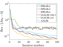
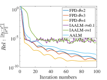
(a) $\emph{subtol}=10^{-6}$

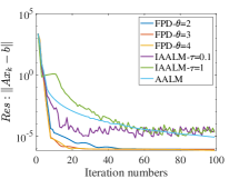
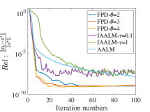
(b) $\emph{subtol}=10^{-8}$

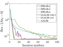
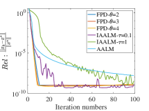
(c) $\emph{subtol}=10^{-10}$

Figure 1: Numerical results of FPD, IAALM and AALM under different tolerance of subproblems

We compare Algorithm 1 (FPD) (update the primal variable by (25)) with IAALM (Kang, Kang, & Jung, 2015, Algorithm 1) ($\mathcal{O}(1/k^{2})$ convergence rate of the Lagrange residual), and AALM (Xu, 2017, Algorithm 1) with adaptive parameters ($\mathcal{O}(1/k^{2})$ convergence rate of the objective residual and the feasibility violation). Set the parameters as follows: FPD: $\alpha=50$, $M=\frac{1}{n}Id$, $\beta_{0}=\frac{0.2}{\theta}$, $\epsilon_{k}=0$ and

$$\beta_{k+1}=\begin{cases}\beta_{k},\quad k<\theta-1;\\ \frac{k}{k+2-\theta}\beta_{k},\quad k\geq\theta-1,\end{cases}$$

where $\theta=\{2,3,4\}$ (In this case, from Lemma 5, the decay rate is $\mathcal{O}(1/k^{\theta})$); IAALM: $\tau=\{0.1,1\}$; AALM: $\gamma=0.1,\ \alpha_{k}=\frac{2}{k+1},\ \beta_{k}=\gamma_{k}=k\gamma,\ P_{k}=\frac{1}{k}Id$.

In Fig. 1, we present the numerical results for various $subtol$ for first $100$ iterations, which demonstrate the superior performance of Algorithm 1 over IAALM and AALM under different $subtol$. We can also observe that the larger $\theta$ is, the better Algorithm 1 performs.

5 Conclusion

By time discretization of the primal-dual dynamical system (3), we propose an accelerated primal-dual algorithm for the linear equality constrained optimization problem, and prove that the algorithm enjoys the fast convergence rate $|f(x_{k})-f(x^{*})|=\mathcal{O}({1}/{k^{2}\beta_{k}})$ and $\|Ax_{k}-b\|=\mathcal{O}({1}/{k^{2}\beta_{k}})$. Further, we prove that the proposed dynamical system owns a fast convergence properties matching to that of the algorithm. We exhibit that the known rates from the literature can be obtained for the second-order dynamical system and the accelerated primal-dual algorithm where only inertial constructions in the sense of Nesterov are needed only for the primal variable. The numerical experiments demonstrate the validity of acceleration and superior performance of the proposed algorithm over some existing ones.

Appendix A Some auxiliary results

The following lemmas have been used in the convergence analysis of the numerical algorithm and the dynamical system.

Lemma 2.

(Attouch et al., 2018, Lemma 5.14) Let $\{a_{k}\}_{k\geq 1}$ and $\{b_{k}\}_{k\geq 1}$ be two nonnegative sequences. Assume $\sum^{+\infty}_{k=1}b_{k}<+\infty$ and

$$a_{k}^{2}\leq c^{2}+\sum^{k}_{j=1}b_{j}a_{j},\quad\forall k\in\mathbb{N},$$

where $c\geq 0$. Then,

$$\sup_{k\geq 1}a_{k}\leq c+\sum^{+\infty}_{j=1}b_{j}<+\infty.$$

Lemma 3.

(Brezis, 1973, Lemma A.5) Let $\nu:[t_{0},T]\to[0,+\infty)$ be integrable and $M\geq 0$. Suppose that $\mu:[t_{0},T]\to\mathbb{R}$ is continuous and

$$\frac{1}{2}\mu(t)^{2}\leq\frac{1}{2}M^{2}+\int^{t}_{t_{0}}\nu(s)\mu(s)ds$$

for all $t\in[t_{0},T]$. Then, $|\mu(t)|\leq M+\int^{t}_{t_{0}}\nu(s)ds$ for all $t\in[t_{0},T]$.

Lemma 4.

Let $\{g_{k}\}_{k\geq k_{0}}$ be a sequence of vectors in $\mathbb{R}^{n}$ and $\{a_{k}\}_{k\geq k_{0}}$ be a sequence in $[0,1)$, where $k_{0}\geq 1$. Assume

$$\left\|g_{k+1}+\sum_{j=k_{0}}^{k}a_{j}g_{j}\right\|\leq C,\quad\forall k\geq k_{0}.$$

Then,

$$\sup_{k\geq k_{0}}\|g_{k}\|<+\infty.$$

Define $\{G_{k}\}_{k\geq k_{0}}$ be a sequence of vectors in $\mathbb{R}^{n}$ as

$$G_{k}=\rho_{k}\sum_{j=k_{0}}^{k}a_{j}g_{j}$$ (33)

with $\rho_{k_{0}}=1$ and

$$\rho_{k+1}=\frac{\rho_{k}}{1-a_{k+1}},\quad\forall k\geq k_{0}.$$

Since $a_{k}\in[0,1)$, $\rho_{k+1}-\rho_{k}=\frac{a_{k+1}\rho_{k}}{1-a_{k+1}}=\rho_{k+1}a_{k+1}\geq 0$. A direct computation leads to

$$G_{k+1}-G_{k} = \rho_{k+1}\sum_{j=k_{0}}^{k+1}a_{j}g_{j}-\rho_{k}\sum_{j=k_{0}}^{k}a_{j}g_{j}$$

$$= \rho_{k+1}a_{k+1}g_{k+1}+(\rho_{k+1}-\rho_{k})\sum_{j=k_{0}}^{k}a_{j}g_{j}$$

$$= (\rho_{k+1}-\rho_{k})(g_{k+1}+\sum_{j=k_{0}}^{k}a_{j}g_{j}),$$

which together with assumption yields

$$\|G_{k+1}-G_{k}\|\leq C(\rho_{k+1}-\rho_{k}),\quad\forall k\geq k_{0}.$$

Using triangle inequality, we get

$$\|G_{k}\| = \|G_{k_{0}}+\sum_{j=k_{0}}^{k-1}(G_{j+1}-G_{j})\|$$

$$\leq \|G_{k_{0}}\|+\sum_{j=k_{0}}^{k-1}\|G_{j+1}-G_{j}\|$$

$$\leq \|G_{k_{0}}\|+C\sum_{j=k_{0}}^{k-1}(\rho_{j+1}-\rho_{j})$$

$$= \|G_{k_{0}}\|+C(\rho_{k}-1)$$

for all $k\geq k_{0}$. Combining (33) and $\rho_{k}\geq 1$ we have

$$\left\|\sum_{j=k_{0}}^{k}a_{j}g_{j}\right\|\leq\|G_{k_{0}}\|+C,\quad\forall k\geq k_{0}.$$

This together with assumption and triangle inequality implies

$$\sup_{k\geq k_{0}}\|g_{k}\|\leq\max\{g_{k_{0}},\|G_{k_{0}}\|+2C\}\leq\|g_{k_{0}}\|+2C<+\infty.$$

Lemma 5.

Let $\{\gamma_{k}\}_{k\geq 1}\subset(0,+\infty)$ be a positive sequence such that $\gamma_{k+1}=(1+\frac{a}{k+b})\gamma_{k}$ for any $k\geq 1$, where $a>0$ and $b\geq 0$. Then, there exist $\mu_{1}>0$ and $\mu_{2}>0$ such that

$$\mu_{1}k^{a}\leq\gamma_{k}\leq\mu_{2}k^{a}.$$

Define $\varphi:[1,+\infty)\to(0,+\infty)$ as

$$\varphi(t)=(k+1-t)\gamma_{k}+(t-k)\gamma_{k+1}=\frac{k+b+a(t-k)}{k+b}\gamma_{k}$$

for any $k\leq t<k+1$. It is easy to verify that $\varphi(t)$ is a positive, piecewise linear and nondecreasing function. By the definition of $\gamma_{k}$, we can compute

$$\dot{\varphi}(t)=\gamma_{k+1}-\gamma_{k}=\frac{a}{k+b}\gamma_{k}=\frac{a}{k+b+a(t-k)}\varphi(t)$$

for any $t\in(k,k+1)$. It yields

$$\frac{\dot{\varphi}(t)}{\varphi(t)}=\frac{a}{(1-a)k+b+at},\quad\forall t\in(k,k+1).$$

Then for any $t\geq 1$, we have

$$\begin{cases}\frac{a}{t+b}\leq\frac{\dot{\varphi}(t)}{\varphi(t)}\leq\frac{a}{t+a+b-1},&0\leq a\leq 1,\\ \frac{a}{t+a+b-1}\leq\frac{\dot{\varphi}(t)}{\varphi(t)}\leq\frac{a}{t+b},&a>1.\end{cases}$$

Since $\varphi(t)$ is a piecewise linear function, integrating the above inequalities over $[0,t]$, we have

$$a\ln(t+b)+C_{1}\leq\ln\varphi(t)\leq a\ln(t+a+b-1)+C_{2}$$

as $0\leq a\leq 1$, and

$$a\ln(t+a+b-1)+C_{1}\leq\ln\varphi(t)\leq a\ln(t+b)+C_{2}$$

as $a>1$, where $C_{1}$ and $C_{2}$ are two constant. It follows that

$$\begin{cases}e^{C_{1}}(t+b)^{a}\leq\varphi(t)\leq e^{C_{2}}(t+a+b-1)^{a},\ &0\leq a\leq 1,\\ e^{C_{1}}(t+a+b-1)^{a}\leq\varphi(t)\leq e^{C_{2}}(t+b)^{a},\ &a>1.\end{cases}$$

As a result, for any $a>0$ there exists $\mu_{1}>0$ and $\mu_{2}>0$ such that $\mu_{1}t^{a}\leq\varphi(t)\leq\mu_{2}t^{a}$. Letting $t=k$ leads to the result.

Lemma 6.

Assume that $g:[t_{0},+\infty)\to\mathbb{R}^{n}$ is a continuous function, $a:[t_{0},+\infty)\to[0,+\infty)$ is a continuous function, $t_{0}>0$, and $C\geq 0$. If

$$\left\|g(t)+\int^{t}_{t_{0}}a(s){g}(s)ds\right\|\leq C,\qquad\forall t\geq t_{0},$$ (34)

then

$$\sup_{t\geq t_{0}}\|{g}(t)\|<+\infty.$$

Define $G:[t_{0},+\infty)\to\mathbb{R}^{n}$ by

$$G(t)=e^{\int^{t}_{t_{0}}a(s)ds}\cdot\int^{t}_{t_{0}}a(s){g}(s)ds.$$ (35)

From (34) and (35), we have

$$\left\|\dot{G}(t)\right\|\leq Ca(t)e^{\int^{t}_{t_{0}}a(s)ds}.$$

Note that $G(t_{0})=0$. It follows that

$$\|G(t)\| = \left\|\int^{t}_{t_{0}}\dot{G}(s)ds\right\|\leq\int^{t}_{t_{0}}\left\|\dot{G}(s)\right\|ds$$

$$\leq \int^{t}_{t_{0}}Ca(s)e^{\int^{s}_{t_{0}}a(h)dh}ds=Ce^{\int^{t}_{t_{0}}a(s)ds}-C.$$

This together with (35) yields

$$\left\|\int^{t}_{t_{0}}a(s){g}(s)ds\right\|\leq C,\quad\forall t\geq t_{0}.$$

From (34) and triangle inequality, we get

$$\sup_{t\geq t_{0}}\|{g}(t)\|\leq 2C<+\infty.$$

The authors would like to thank the reviewers and the editors for their helpful comments and suggestions, which significantly improve the quality of this paper. In particular, we would like to thank one reviewer for sharing Lemma 4 and Lemma 5 with us, which have made the results better.

References

• Attouch et al. (2018) Attouch, H., Chbani, Z., Peypouquet, J., & Redont, P. (2018). Fast convergence of inertial dynamics and algorithms with asymptotic vanishing viscosity. Mathematical Programming, 168(1), 123-175.
• Attouch, Chbani, & Riahi (2019) Attouch, H., Chbani, Z., & Riahi, H. (2019). Fast proximal methods via time scaling of damped inertial dynamics. SIAM Journal on Optimization, 29(3), 2227-2256.
• Attouch et al. (2022) Attouch, H., Chbani, Z., Fadili, J., & Riahi, H. (2022). Fast convergence of dynamical ADMM via time scaling of damped inertial dynamics. Journal of Optimization Theory and Applications, 193(1-3), 704–736.
• Beck & Teboulle (2009) Beck, A., & Teboulle, M. (2009). A fast iterative shrinkage-thresholding algorithm for linear inverse problems. SIAM Journal on Imaging Sciences, 2(1), 183-202.
• Boyd et al. (2011) Boyd, S., Parikh, N., Chu, E., Peleato, B., & Eckstein, J. (2011). Distributed optimization and statistical learning via the alternating direction method of multipliers. Foundations and Trends in Machine Learning, 3(1), 1-122.
• Boţ & Nguyen (2021) Boţ, R. I., & Nguyen, D. K. (2021). Improved convergence rates and trajectory convergence for primal-dual dynamical systems with vanishing damping. Journal of Differential Equations, 303, 369-406.
• Boţ, Csetnek, & Nguyen (2021) Boţ, R. I., Csetnek, E. R., & Nguyen, D. K. (2021). Fast Augmented Lagrangian Method in the convex regime with convergence guarantees for the iterates. arXiv:2111.09370.
• Brezis (1973) Brezis, H. (1973). Operateurs maximaux monotones et semi-groupes de contractions dans les espaces de Hilbert. Elsevier, New York.
• Candès & Wakin (2008) Candès, E. J., & Wakin, M. B. (2008). An introduction to compressive sampling. IEEE Signal Processing Magazine, 25(2), 21-30.
• Chen & Luo (2021) Chen, L., & Luo, H. (2021). A unified convergence analysis of first order convex optimization methods via strong Lyapunov functions. arXiv:2108.00132.
• Fazlyab et al. (2017) Fazlyab, M., Koppel, A., Preciado, V. M., & Ribeiro, A. (2017). A variational approach to dual methods for constrained convex optimization. In 2017 American Control Conference (ACC) (pp. 5269-5275). IEEE.
• Feijer & Paganini (2010) Feijer, D., & Paganini, F. (2010). Stability of primal–dual gradient dynamics and applications to network optimization. Automatica, 46(12), 1974-1981.
• Haraux (1991) Haraux, A. (1991). Systemes dynamiques dissipatifs et applications. Elsevier Masson.
• He, Hu, & Fang (2021a) He, X., Hu, R., & Fang, Y. P. (2021a). Convergence rates of inertial primal-dual dynamical methods for separable convex optimization problems. SIAM Journal on Control and Optimization, 59(5), 3278-3301.
• He, Hu, & Fang (2021b) He, X., Hu, R., & Fang, Y. P. (2021b). Fast convergence of primal-dual dynamics and algorithms with time scaling for linear equality constrained convex optimization problems. arXiv:2103.12931v2.
• He, Hu, & Fang (2022) He, X., Hu, R., & Fang, Y. P. (2022). Inertial accelerated primal-dual methods for linear equality constrained convex optimization problems. Numerical Algorithms, DOI:10.1007/s11075-021-01246-y.
• He & Yuan (2010) He, B., & Yuan, X. (2010). On the acceleration of augmented Lagrangian method for linearly constrained optimization. Optimization online, 3. http://www.optimization-online.org/DB_FILE/2010/10/2760.pdf.
• Huang, Ma, & Goldfarb (2013) Huang, B., Ma, S., & Goldfarb, D. (2013). Accelerated linearized Bregman method. Journal of Scientific Computing, 54(2), 428-453.
• Jordan (2018) Jordan, M. I. (2018). Dynamical, symplectic and stochastic perspectives on gradient-based optimization. In Proceedings of the International Congress of Mathematicians: Rio de Janeiro 2018 (pp. 523-549).
• Kang, Kang, & Jung (2015) Kang, M., Kang, M., & Jung, M. (2015). Inexact accelerated augmented Lagrangian methods. Computational Optimization and Applications, 62(2), 373-404.
• Kang et al. (2013) Kang, M., Yun, S., Woo, H., & Kang, M. (2013). Accelerated Bregman method for linearly constrained $\ell_{1}$-$\ell_{2}$ minimization. Journal of Scientific Computing, 56(3), 515-534.
• Kia, Cortés, & Martínez (2015) Kia, S. S., Cortés, J., & Martínez, S. (2015). Distributed convex optimization via continuous-time coordination algorithms with discrete-time communication. Automatica, 55, 254-264.
• Liang & Yin (2019) Liang, S., & Yin, G. (2019). Exponential convergence of distributed primal–dual convex optimization algorithm without strong convexity. Automatica, 105, 298-306.
• Lin, Li, & Fang (2020) Lin, Z., Li, H., & Fang, C. (2020). Accelerated optimization for machine learning. Springer Singapore.
• Luo (2022) Luo, H. (2022). A primal-dual flow for affine constrained convex optimization. ESAIM: Control, Optimisation and Calculus of Variations, 28, Article Number: 33.
• Luo (2021a) Luo, H. (2021a). A unified differential equation solver approach for separable convex optimization: splitting, acceleration and nonergodic rate. arXiv:2109.13467.
• Luo (2021b) Luo, H. (2021b). Accelerated primal-dual methods for linearly constrained convex optimization problems. arXiv:2109.12604.
• Nesterov (1983) Nesterov, Y. (1983). A method of solving a convex programming problem with convergence rate $\mathcal{O}(1/k^{2})$. In Sov. Math. Dokl, 27(2), 372-376.
• Nesterov (2003) Nesterov, Y. (2003). Lectures on Convex Optimization: A basic course. Springer Science & Business Media.
• Su, Boyd, & Candès (2016) Su, W., Boyd, S., & Candès, E. J. (2016). A differential equation for modeling nesterov’s accelerated gradient method: Theory and insights. Journal of Machine Learning Research, 17(153), 5312-5354.
• Wang et al. (2021) Wang, Z., Wei, W., Zhao, C., Ma, Z., Zheng, Z., Zhang, Y., & Liu, F. (2021). Exponential stability of partial primal–dual gradient dynamics with nonsmooth objective functions. Automatica, 129, 109585.
• Wibisono, Wilson, & Jordan (2016) Wibisono, A., Wilson, A. C., & Jordan, M. I. (2016). A variational perspective on accelerated methods in optimization. Proceedings of the National Academy of Sciences, 113(47), E7351-E7358.
• Wilson, Recht, & Jordan (2021) Wilson, A. C., Recht, B., & Jordan, M. I. (2021). A Lyapunov analysis of accelerated methods in optimization. Journal of Machine Learning Research, 22(113), 1-34.
• Xu (2017) Xu, Y. (2017). Accelerated first-order primal-dual proximal methods for linearly constrained composite convex programming. SIAM Journal on Optimization, 27(3), 1459-1484.
• Yan & He (2020) Yan, S. He, N. (2020). Bregman augmented Lagrangian and its acceleration. arXiv:2002.06315.
• Zeng, Lei, & Chen (2022) Zeng, X., Lei, J., & Chen, J. (2022). Dynamical primal-dual accelerated method with applications to network optimization. IEEE Transactions on Automatic Control, DOI:10.1109/TAC.2022.3152720.
• Zhang et al. (2010) Zhang, X., Burger, M., Bresson, X., & Osher, S. (2010). Bregmanized nonlocal regularization for deconvolution and sparse reconstruction. SIAM Journal on Imaging Sciences, 3(3), 253-276.
• Zhu et al. (2020) Zhu, Y., Yu, W., Wen, G., & Chen, G. (2020). Projected primal–dual dynamics for distributed constrained nonsmooth convex optimization. IEEE Transactions on Cybernetics, 50(4), 1776-1782.