Danish Fungi 2020 – Not Just Another Image Recognition Dataset

Abstract

We introduce a novel fine-grained dataset and benchmark, the Danish Fungi 2020 (DF20). The dataset, constructed from observations submitted to the Atlas of Danish Fungi, is unique in its taxonomy-accurate class labels, small number of errors, highly unbalanced long-tailed class distribution, rich observation metadata, and well-defined class hierarchy. DF20 has zero overlap with ImageNet, allowing unbiased comparison of models fine-tuned from publicly available ImageNet checkpoints. The proposed evaluation protocol enables testing the ability to improve classification using metadata – e.g. precise geographic location, habitat, and substrate, facilitates classifier calibration testing, and finally allows to study the impact of the device settings on the classification performance. Experiments using Convolutional Neural Networks (CNN) and the recent Vision Transformers (ViT) show that DF20 presents a challenging task. Interestingly, ViT achieves results superior to CNN baselines with 80.45% accuracy and 0.743 macro F1 score, reducing the CNN error by 9% and 12% respectively. A simple procedure for including metadata into the decision process improves the classification accuracy by more than 2.95 percentage points, reducing the error rate by 15%. The source code for all methods and experi- ments is available at https://sites.google.com/view/danish-fungi-dataset.

1 Introduction

Publicly available datasets and benchmarks accelerate machine learning research and allow for quantitative comparison of novel methods. In the area of deep learning and computer vision, the rapid progress over the past decade was, to a great extent, facilitated by the publication of large-scale image datasets. In the case of image recognition, the formation of the ImageNet [7] database and its usage in the ILSVRC challenge [36], together with PASCAL VOC [10] among others, helped start the CNN revolution. The same holds for the problem of fine-grained visual categorization (FGVC), where datasets and challenges like PlantCLEF [13, 14, 22], iNaturalist [46], CUB [48], and Oxford Flowers  [33], have helped to develop and evaluate novel approaches to fine-grained domain adaptation [12], domain specific transfer learning [17], image retrieval [34, 38, 53], unsupervised visual representation, few-shot learning  [49], transfer learning [17], prior-shift [39] and many others.

Figure 1: Selected images from the DF20 dataset from different Habitats (Rows) that grow on a variety of Substrates (Columns).

While the datasets have been extremely useful for the image recognition community, there are issues that limit their relevance to real-world applications. We mention several such problems. Uniform class distribution, common in research datasets, are rare in practice. Often, class prior distributions are the same in the training and test splits. This is a standard machine learning assumption that, nevertheless, is not valid if the collection of training data differs from the deployment of the trained system, which is not rare. A non-negligible percentage of noisy-labels restricts quality assessment [3], and, despite CNN’s surprising robustness to label noise [24], may influence the perceived relative merit of learning algorithms. Some commonly used datasets [7, 25, 33] are saturated in accuracy or close to the point, leaving limited space for improvement in future research [3]. Extremely large dataset sizes might discourage researchers that do not have access to massive computational resources as experiments have become time and hardware demanding.

	# Classes	# Training	# Testing
FGVC-Aircafts [32]	102	6,732	3,468
Standford Cars [25]	196	8,144	8,041
VMMRdb [42]	9,170	291,752	$\times$
Oxford Flowers [33]	102	1,020	7,169
Stanford Dogs [30]	120	12,000	8,580
DogSnap [30]	133	4,776	3,575
LeafSnap [27]	185	30,866	$\times$
CUB 200-2011 [48]	200	5,994	5,784
VegFru [20]	292	29,200	116,931
Birdsnap [2]	500	47,386	2,443
NABirds [45]	555	48,562	$\times$
PlantCLEF 2015 [22]	1,000	91,758	21,446
iNaturalist 2017 [46]	5,089	579,184	95,986
PlantCLEF 2017† [14]	10,000	230,658	25,629
DF20 - Mini	182	32,753	3,640
DF20	1,604	266,344	29,594

Table 1: Overview of publicly available FGVC datasets, nature-related (middle section) and other (top), and the number of images and categories. ^† Images with “clean” (accurate) labels only.

With these observations in mind, we introduce the DF20 dataset with a number of unique characteristics. Its class labels are exceptionally accurate, annotated by domain experts – Mycologists with specialization on specific Families/Genera. Moreover, we are preparing private test with labels acquired by DNA sequencing. The minimal error levels allow highly accurate performance evaluation. With its zero overlap with ImageNet, it allows an unbiased comparison of models fine-tuned from publicly available ImageNet checkpoints.

The class frequencies in DF20 follow the natural species distribution, which is long-tailed. The frequencies change significantly within the calendar year, making the data suitable for testing the response of the classifier to differing long tailed distributions and changing class priors. The continuous data flow of collection over a long period provides a ground for modelling and exploiting the temporal phenomena on different scales, e.g., month, season, year.

The visual data is accompanied with metadata for more than 99% of the image observations. The rich metadata includes information related to the environment, place, time and full taxonomy labels and enables testing the ability to improve classification accuracy using different metadata types – time, precise location, habitat, and substrate type, to perform hierarchical classification, evaluate fine-grained classification on different levels of granularity (taxonomic ranks), to test classifier calibration, and to model intra-metadata and metadata-visual appearance relationships. Moreover, EXIF metadata is available for many observations, which is useful, e.g., for studying the impact of the device settings on classification performance.

The DF20 Benchmark. To allow evaluation at any time, we have prepared a web-based public automatic benchmark  for different scenarios, including visual-based, metadata focused or classifier-calibration related research. Besides the full benchmark, we introduce DF20 - mini, a small subset with roughly 1/10 of the data and species, for fast, low-energy friendly prototyping. DF20 - mini includes six well-known genera of fungi forming fruit-bodies of the toadstool type, and offers, surprisingly, an even more challenging problem then the full benchmark, while having a compact size.

We prepared a baseline performance evaluation, including the quantitative and qualitative analysis of the results for a number of well-known CNN and recent ViT architectures [8]. The recent ViT achieves excellent results in fine-grained classification outperforming the state-of-the-art CNN classifiers. We show that ViT performs way better on the FGVC domain, where attention to detail is needed, than in a common object recognition. We show that both the DF20 and DF20 - Mini benchmarks are far from saturated as the best performing model - ViT-Large/16-384 - achieved 80.45% and 75.85% accuracy on DF20 and DF20 - Mini, respectively. We propose a simple method for processing the habitat, substrate and time (month) metadata, showing that – even with the simple approach – utilizing the metadata increases the classification performance significantly. To support and accelerate future research on the DF20 we open source the code through the public GitHub.

Russula	Russula	Russula	Hortiboletus	Suillellus	Neoboletus	Amanita	Amanita	Amanita
emetica	paludosa	rosea	rubellus	queletii	luridiformis	muscaria	rubescens	pantherina

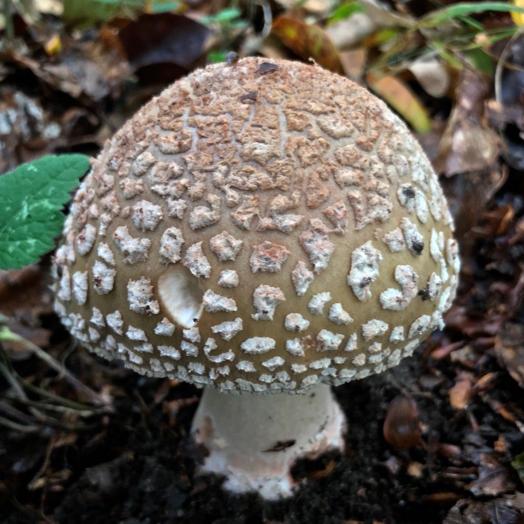
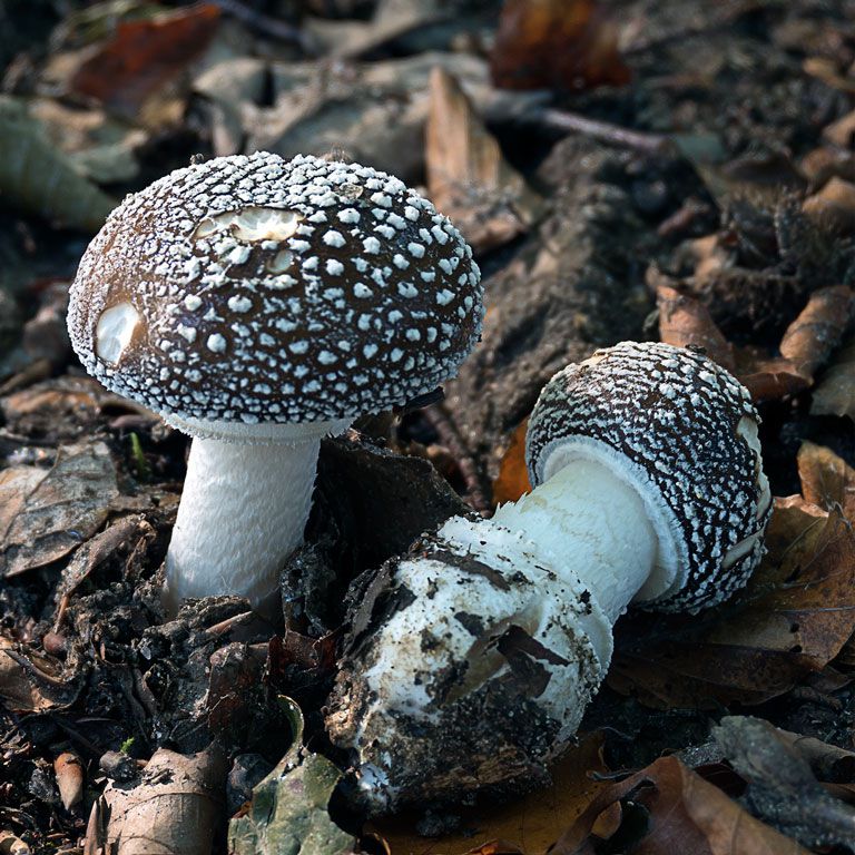
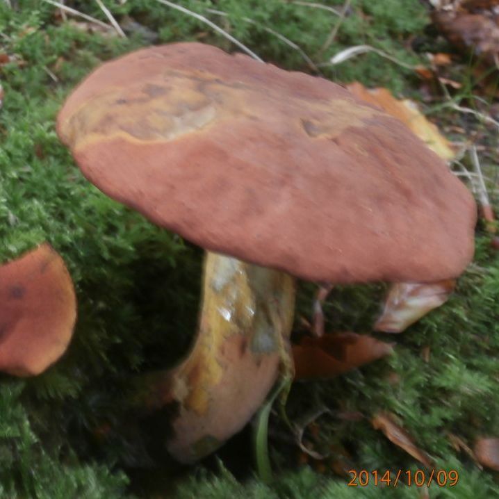
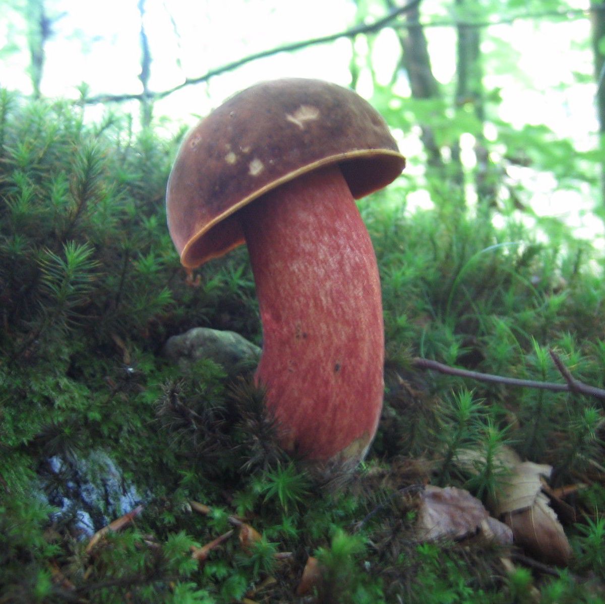
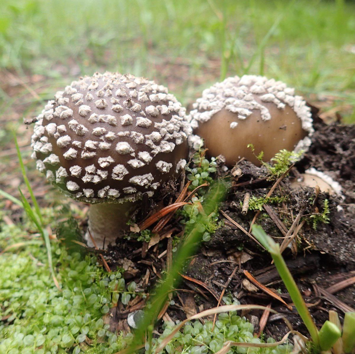
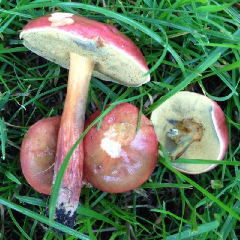
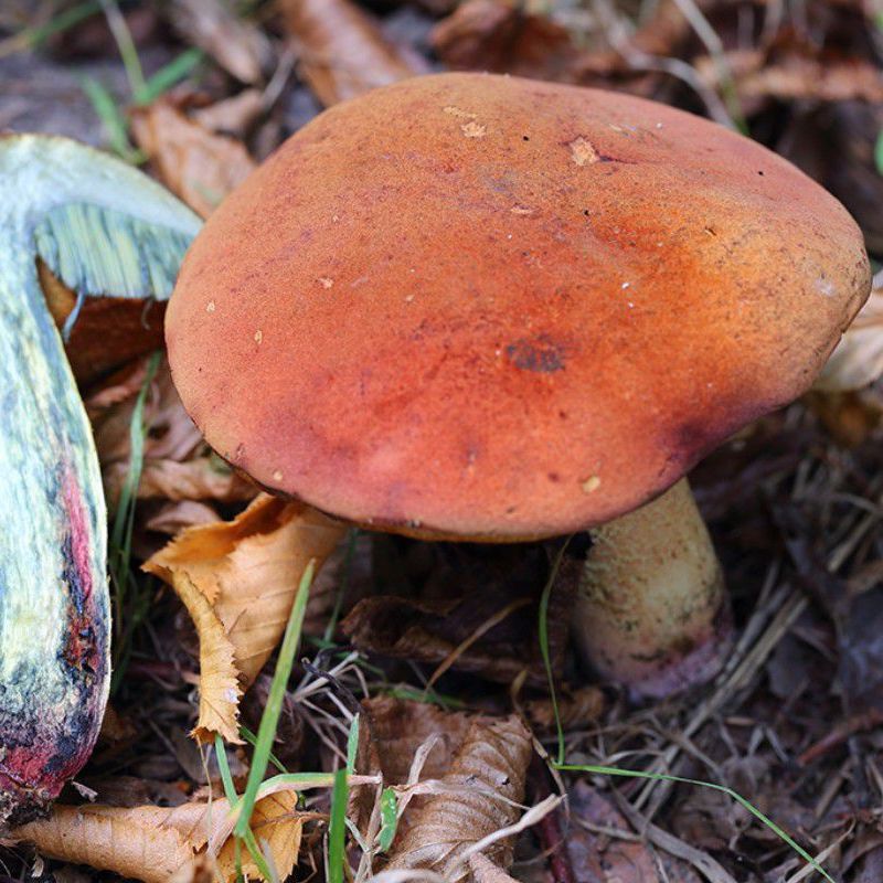
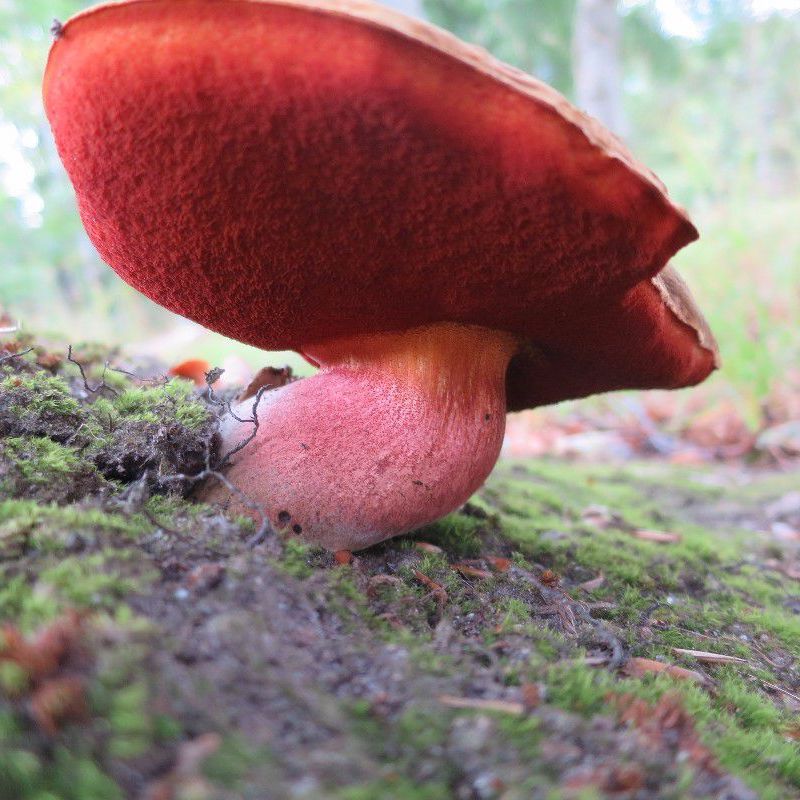
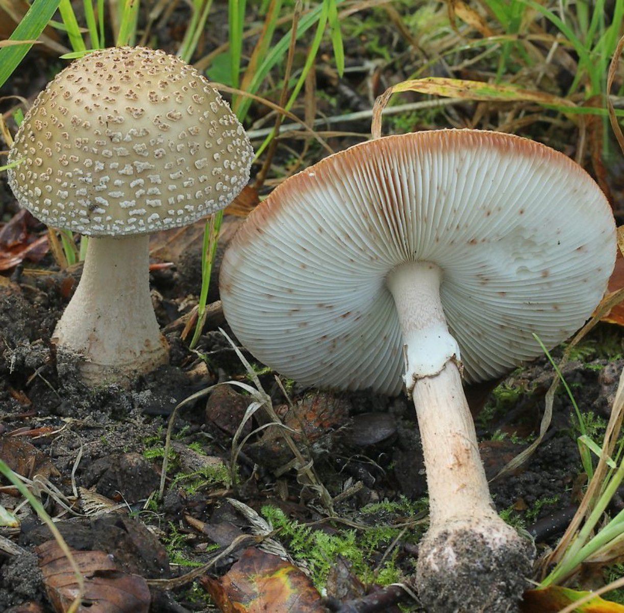
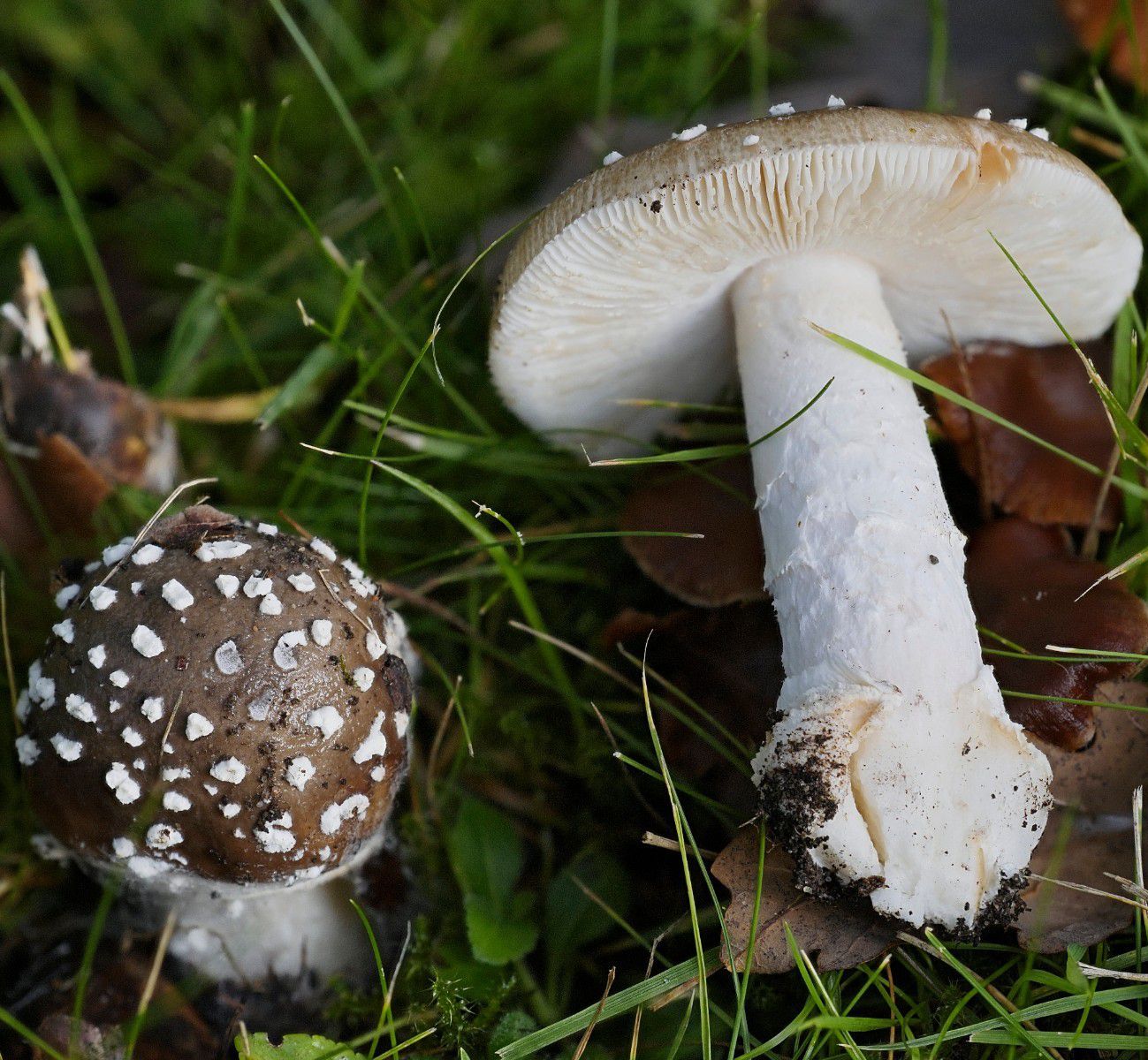
Figure 2: Examples of intra- and inter-class similarities and differences for selected species of three taxonomically distinct fungi families. The similarity holds on the species and the family level. Left: Russulaceae, center: Boletaceae, right: Amanitaceae.

2 Related Work

This section overviews existing fine-grained image datasets, which, unlike datasets with visually distinct object classes [10, 26], are characterized by small inter-class differences and huge intra-class similarity. Currently, there exists a number of FGVC dataset with a focus on plants [14, 20, 22, 27, 33], animals [2, 23, 45, 48], cars [25, 42] or airplanes [32]. The dataset statistics are compared in Table 1. Most of the datasets are artificially constructed to have a flat class distribution. Many datasets use web scraped data that may contain out-of-domain images and wrong labels.

Fungi species have been covered by image classification datasets. In the FGVCx 2018 Fungi classification challenge , a dataset sampled from the same source as DF20 was used. The challenge dataset was smaller, scrambled the species names, did not include taxonomic labels and did not contain any metadata. The latest edition of iNaturalist dataset includes 90,048 images of 384 fungi species from 240 genera. DF20 is more fine-grained in the Fungi kingdom, and it is thus more challenging, with more than 1,500 fungi species. Many of these visually similar but from different genera or families (Figure 2).

Labels. As species-level labels are essential for usage in real-world applications, the tedious labelling procedure often rely on domain experts. With just a small number of experts and their limited time, the labelling process is frequently delegated to crowd-sourced annotation platforms such as the Amazon Mechanical Turk [7, 23, 48]. The main drawback of this approach is related to poor domain knowledge of the annotators that results in a high number of noisy labels [45] – 4.4% in CUB 200-2011 and approximately 4.0% for fine-grained classes in ImageNet. To address this issue, more recent datasets use citizen-science platforms and their users – citizen scientists – to label data with high-quality annotations [45, 46].

ImageNet Overlap. Strict separation of training and test data is a core machine learning principle and it is standard in the field of image recognition. Nevertheless, some datasets containt ImageNet images in their test set, and thus fine-tuning from ImageNet weights contradicts the separation principle. This is commonly overlooked and may lead to biased (inflated) test set accuracies. For instance, a number of publications with high impact used ImageNet weights and performed the fine-tuning and testing with the CUB 200-2011 [48] dataset that overlaps with the ImageNet [4, 28, 29, 34, 51, 52, 54, 55, 56] in 43 out of 5,794 images (0.75%).

Metadata. Besides images and class labels, image classification datasets often provide additional metadata, such as higher taxon labels [22, 46], label hierarchy [7, 20, 32], object parts and attribute annotations [22, 45, 48], masks [48], GPS location [22], and time of observation [22]. The existence of such metadata enables the usage of these datasets in machine learning research beyond image classification. For example [1, 9, 31] use location context, and  [15] use taxonomy labels.

3 Atlas of Danish Fungi

The Atlas of Danish Fungi (Svampeatlas) [6, 11, 19] is supported by more than 3,300 volunteers who have contributed more than 950,000 content-checked observations of fungi, many with expert-validated class labels, submitted mostly since 2009.

The project has resulted in a vastly improved knowledge of fungi in Denmark [19]. More than 180 species belonging to Basidiomycota  have been added to the list of known Danish species, and several species that were considered extinct have been re-discovered. Simultaneously, several search and assistance functions have been developed that present features relating to the individual species, making it much easier to include an understanding of endangered species in nature management and decision-making.

Expert-validated Svampeatlas records are published in the Global Biodiversity Information Facility (GBIF), weekly, since 2017. As of end of July 2021, GBIF included 438,872 such images.

3.1 Annotation Process

The Atlas of Danish Fungi uses an interactive labelling procedure for all submitted observations. When a user submits a fungal sighting (record) at species level, a ”reliability score” (1–100) is calculated based on following factors:

• Species rarity, i.e. its relative frequency in the Atlas.

• The geographical distribution of the species.

• Phenology of the species, its seasonality.

• User’s historical species-level proposal precision.

• As above, within the proposal’s higher taxon rank.

Subsequently, other users may agree with the proposed species identity, increasing the identification score following the same principles, or proposing alternative identification for non-committal suggestions. Once the submission reaches a score of 80, the label (identification) is internally approved. Simultaneously, a small group of taxonomic experts (validators) monitor most of the observation on their own. These have the power to approve or reject species identifications regardless of the score in the interactive validation. Since 2019, the Atlas of Danish Fungi observation identification has been streamlined thanks to an image recognition system [40].

Fungi	Protozoa	Fungi	Chromista

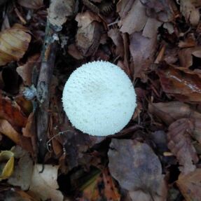
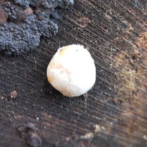
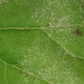
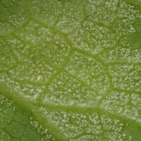
Figure 3: Visually similar image pairs from the Fungi and Protozoa, and from the Fungi and Chromista kingdoms, respectively.

4 Dataset Description

The Danish Fungi 2020 (DF20) dataset contains image observations from the Atlas of Danish Fungi belonging to species with more than 30 images. The data are observations collected before the end of 2020 , originating from 30 countries, and including samples from all seasons. It consists of 295,938 images belonging to 1,604 species mainly from the Fungi kingdom with a few visually similar species (See Figure 3) from Protozoa (1.7% classes / 1.1% images) and Chromista kingdoms (0.06% classes / 0.03% images) kingdoms, covering 566 genera and 190 families. The most frequent species – Trametes versicolor – is represented by 1,913 images and the least present with 31.

	Images	Species	Genera	Families
Svampeatlas (GBIF)	438,872	6,347	1,519	398
DF20	295,938	1,604	566	190
DF20 - Mini	36,393	182	6	6

Table 2: Numbers of images, species, genera and families in the Atlas of Danish Fungi and their subsets DF20 and DF20 - Mini.

Additionally, we hand-picked a subset of 36,393 images belonging to 182 species from 6 genera with a similar visual appearance. This compact dataset, DF20 - Mini, introduces a challenging fine-grained recognition task, while allowing to decrease the necessary training times and hardware requirements. As species in the same genus are most likely to be confused, we chose six commonly known genera of fungi forming fruit-bodies of the toadstool type with a large number of species: (Russula, Boletus, Amanita, Clitocybe, Agaricus and Mycena) for the construction of the DF20 - Mini. The most frequent species in the DF20 - Mini dataset – Mycena galericulata – has 1,221 images, the rarest have 31 samples. For a quantitative summary of the data selection, see Table 2.

The DF20 and DF20 - Mini datasets were randomly split – with respect to the class distribution – into the provided training and (public) test sets, where the training set contains $\lceil 90\%\rceil$ of images of each species.

Figure 4: Monthly distribution of observations in the DF20 dataset for genera Mycena, Boletus, and Exidia. The differences imply that the class prior distribution varies significantly over time.

4.1 Metadata

Unlike most computer vision datasets, DF20 and DF20 - Mini include rich metadata acquired by citizen-scientists in the field while recording the observations. We see a promising research direction in combining visual data with metadata like timestamp, location at multiple scales, substrate, habitat, full taxonomy labels and camera device settings. For a detailed list see Table 4.

Substrate. Substrates on which fungi live and fruit are an important source of information that helps differentiate similarly looking species. Each species or genus has its preferable substrate, and it is rare to find it on other substrates. For example, Trametes occurs only on wood and Russula on soil. As such metadata is crucial for the final categorization capability, we provide one of 32 substrate types for more than 99% of images. We differentiate wood of living trees, dead wood, soil, bark, stone, fruits, mosses and others.

Location. Fungi are highly location dependent with different species distributions across continents, states, regions or even districts. To support studies on better understanding where Fungi species lives, we include multi-level location information. Starting from latitude and longitude values and their uncertainty, we further extracted information about the country, region, district, and locality with 9003 unique values.

Time-Stamp. Time of observation is essential for fungi classification in the wild as fruitbodies’ presence depends on seasonality or even (but rarely) the time in a day. Considering the existence of such dependency, integrating information about time into the classification should also improve fungal recognition. In Figure 4 we show the probability of three genera being observed in different months of the calendar year. Brief inspection shows that there is almost zero probability to spot a Boletus in January but still a small chance to find a Mycena. In contrast to Boletus, Exidia occurs mostly during the cold months.

EXIF data. Since the camera device and its settings affect the resulting image, the image classification models may be biased towards certain (e.g. more common) device attributes. To allow a deeper study of such phenomena, we include the EXIF data for approximately 84% of images, where the EXIF information was available in the Atlas of Danish Fungi. The included attributes, the number of unique values in the dataset and the proportion of images with the attributes present are summarized in Table 3.

Attribute	Coverage [%]	# Values
White Balance	79.99	2
Color Space	84.38	3
Metering Mode	78.23	10
SceneCaptureType	81.04	13
Compressed Bits Per Pixel	37.75	88
Aperture Value	46.63	297
Device	80.31	688
Focal Length	80.13	1,580
Exposure Time	80.12	4,594
Shutter Speed Value	46.78	7,079

Table 3: Device settings extracted from the original image EXIFs in the Atlas of Danish Fungi, with the proportion of images where the attributes are present (Coverage), and the number of unique values of the attribute in the dataset.

Habitat. While substrate denotes the spots, the habitat indicates the more overall environment where fungi grow and hence is vital for fungal recognition. It is well known that some species occur in deciduous forests rather than in conifer forests or plantations, while others grow in farmland. For a deeper understanding of such relation, we include the information about the habitat for approximately 99.5% of observations.

Attribute	Description
EventDate	Date of observation.
EXIF	Camera device attributes extracted from the image, e.g., metering mode, color space, device type, exposure time, and shutter speed.
Habitat	The environment where the specimen was observed. Selected from 32 values such as Mixed woodland, Deciduous woodland etc.
Substrate	The natural substance on which the specimen lives. A total of 32 values such as Bark, Soil, Stone, etc.
Scientific	Lowest taxonomic rank including specific Epithets. 1,604 unique values present.
Species	1th taxon rank. 1,578 unique values present.
Genus	2nd taxon rank. 566 unique values present.
Family	3rd taxon rank. 190 unique values present.
Order	4th taxon rank. 66 unique values present.
Class	5th taxon rank. 23 unique values present.
Phylum	6th taxon rank. 5 unique values present.
Kingdom	7th taxon rank. 3 unique values present.
CountryCode	ISO 3166-1 alpha-2 code (DK, AT, etc.) of the observation. The dataset covers 30 countries.
Locality	More precise location information. Mostly smaller than a district, e.g. part of a city or a specific forest. 9003 values present.
Level1Gid	ID of a Country region related to the specimen observation, 115 regions are listed.
Level2Gid	ID of a district region related to the specimen observation, 317 districts are listed.
Latitude	A decimal GPS coordinate.
Longitude	A decimal GPS coordinate.
GPSUncert	GPS coordinates uncertainty in meters.

Table 4: Description of the provided metadata (observation attributes). For almost all images, a detailed information about taxonomy, location, time, habitat and substrate type is included.

5 Experiments

To establish a baseline performance on the DF20 and DF20 - Mini datasets, we performed multiple experiments. First, we train a wide variety of well known CNN architectures such as ResNets [18], EfficientNets [43], MobileNet [37], Inception networks [41] and SE-ResNeXt-101-32x4d that extends the ResNet-101 by cardinality [50] and Squeeze and Excite blocks [21]. Second, the EfficientNet-B0, EfficientNet-B3, and SE-ResNeXt-101-32x4d are compared with Vision Transformer architectures ViT-Large/16 and ViT-Base/16 [8]. Finally, the impact of different metadata and their combinations on both the CNN and the ViT final prediction performance is evaluated.

5.1 Setup

In this section, we describe the full training and evaluation procedure, including the training strategy and image augmentations.

Training Strategy. All architectures were initialized from publicly available ImageNet-1k pre-trained checkpoints and further fine-tuned with the same strategy for 100 epochs with the PyTorch framework [35] within the 21.05 NGC deep learning framework Docker container. All neural networks were optimized by Stochastic Gradient Descent with momentum set to 0.9. The start Learning Rate (LR) was set to 0.01 and was further decreased with a specific adaptive learning rate schedule strategy – if the validation loss is not reduced from one epoch to another, reduce LR by 10%. To have the same effective mini-batch size of 64 for all architectures, we accumulated gradients from smaller mini-batches accordingly, where needed.

Augmentations. For training, we utilized several augmentation techniques from the Albumentations library [5]. More specifically, we used: random horizontal flip with 50% probability, random vertical flip with 50% probability, random resized crop with a scale of 0.8 - 1.0, random brightness / contrast adjustments with 20% probability, and mean and std. dev. normalization. All images were resized to the required network input size: For the CNN performance experiment, inputs of size 299$\times$299 were used. In the case of the CNN vs ViT experiment, we used two different resolutions, 224$\times$224 and 384$\times$384, to match the input resolutions of the pre-trained models.

Test-time. While testing, we avoided any additional techniques such as ensembles, centre-cropping, prior weighting, etc. Only the resize and normalization operations were used to pre-process the data. The impact of test-time augmentation methods on the final performance can be studied in the future.

5.2 Metadata Use

We propose a simple method for the use of metadata to improve the categorization performance – similar to spatio-temporal prior used in [2]. For a given type of metadata ($D$) and image ($I$), we adopt the following assumption for the likelihood of an image observation:

$$\small P(I|S)=P(I|S,D),$$ (1)

i.e. that the visual appearance of a species does not depend on the metadata. This does not mean that the posterior probability of a species given an image is independent of metadata $D$.

A few lines of algebraic manipulation prove that under assumption Eq. (1), the class posterior given the image $I$ and metadata $D$ is easily obtained:

$$P(S|I,D) =P(S|I)\frac{P(S|D)}{P(S)}\frac{P(I)}{P(I|D)}$$ (2)

$$\propto P(S|I)\frac{p(S|D)}{p(S)},$$

where $P(S)$ is the class prior in the training set. The discrete conditional probability $P(S|D)$ is estimated as the relative frequency of species $S$ with metadata $D$ in the training set.

While we know this assumption is not always true in practice, since metadata like substrate or time in fact do impact the image background as well as the appearance of the specimen, this is the only possible approach not requiring modelling the dependence of visual appearance and the metadata. The model trained without metadata has no information about visual appearance changes of a species as a function of $D$. Moreover, this assumption is applicable for situations where the classifier has to be treated as a black box without the possibility to retrain the model. Even this simplistic model based on an unrealistic assumption reduces error rates, see Table 7.

With multiple metadata at once, e.g. month and habitat, we combine the posteriors assuming statistical independence:

$$\small P(S|D_{1},D_{2})\propto\frac{P(S|D_{1})P(S|D_{2})}{P(S)}.$$ (3)

This is a simple, baseline assumption, which again may not always be valid for related meta-data. Direct estimation of $P(S|D_{1},D_{2})$, e.g. as relative frequencies, is another possibility. The D20 benchmark has thus the potential to be a fertile ground for evaluation of intra-metadata, as well as visual-metadata, dependencies.

The approach of Eq. (2) needs a probabilistic classifier to serve as an estimator of $P(S|I)$. In our experiments, we use the outputs of the softmax layer. Note that for CNNs, the estimates of $\max P(S|I)$ are typically overconfident, and the quality of the estimator can be improved by a process is called calibration in the literature [16, 44]. The proposed benchmark may be used, in the context of exploiting metadata, to evaluate and compare classifier calibration techniques.

5.3 Metrics

	Top1	Top3	$\text{F}_{1}^{m}$	Top1	Top3	$\text{F}_{1}^{m}$
MobileNet-V2	65.58	83.65	0.550	69.77	85.01	0.606
ResNet-18	62.91	81.65	0.514	67.13	82.65	0.580
ResNet-34	65.63	83.52	0.559	69.81	84.76	0.600
ResNet-50	68.49	85.22	0.587	73.49	87.13	0.649
EfficientNet-B0	67.94	85.71	0.567	73.65	87.55	0.653
EfficientNet-B1	68.35	84.67	0.572	74.08	87.68	0.654
EfficientNet-B3	69.59	85.55	0.590	75.69	88.72	0.673
EfficientNet-B5	68.76	85.00	0.579	76.10	88.85	0.678
Inception-V3	65.91	82.97	0.535	72.10	86.58	0.630
Inception-ResNet-V2	64.67	81.42	0.542	74.01	87.49	0.651
Inception-V4	67.45	82.78	0.560	73.00	86.87	0.637
SE-ResNeXt-101	72.23	87.28	0.620	77.13	89.48	0.693
	DF20 - Mini			DF20

Table 5: Classification performance of selected CNN architectures on DF20 and DF20 - Mini. All networks share the settings described in Section 5.1 and were trained on 299$\times$299 images. The top results – $\text{F}_{1}^{m}$, see Eq. (4), equal to 0.620 / 0.693 and Top1 to 72.23% / 77.13% – are far from saturated. The datasets are challenging for the state-of-the-art CNN classifiers.

Besides commonly used metrics, Top1 and Top3 accuracy, we measured the macro-averaged $\text{F}_{1}$ score, $\text{F}_{1}^{m}$, which is not biased by class frequencies and is more suitable for the long-tailed class distributions observed in the nature. Interestingly, even though the performance across the whole taxonomy in nature-related FGVC datasets is highly demanded, most existing datasets are only using accuracy as the score measure. Considering that the datasets are highly imbalanced with long-tail distribution, learning procedure may ignore the least present species. Additionaly, usage of $\text{F}_{1}^{m}$ allows to easily assign a cost value to both types of error (fp and fn) for each label and to measure more task-relevant performance. For example, in fungi recognition, mistaking a poisonous mushroom for the edible one is a more significant problem than the opposite.

The $\text{F}_{1}^{m}$ is defined as the mean of class-wise $\text{F}_{1}$ scores:

$$\small\text{F}_{1}^{m}=\frac{1}{N}\sum_{S=1}^{N}F_{1_{S}}\,,$$ (4)

where $N$ represents the number of classes and $S$ is the species index. Than the $\text{F}_{1}$ score for each class is calculated as a harmonic mean of the class precision $P_{S}$ and recall $R_{S}$:

$$\small F_{1_{S}}=2\times\frac{{P_{S}}\times{R_{S}}}{P_{S}+R_{S}}\,,$$ (5)

$$\small P_{S}=\frac{\text{\it tp}_{S}}{\text{\it tp}_{S}+\text{\it fp}_{S}}\,,\,R_{S}=\frac{\text{\it tp}_{S}}{\text{\it tp}_{S}+\text{\it fn}_{S}}\,$$ (6)

In multi-class classification, the True Positive (tp) represents the number of correct Top1 predictions, False Positive (fp) how many times was a specific class predicted instead of the (tp), and False Negative (fn) how many images of class $S$ have been misclassified.

5.4 Results

In this section, we compare the performance of the well known CNN based models and ViT models in terms of Top1 and Top3 accuracy, and the newly included $\text{F}_{1}^{m}$ metric. Additionally, we discuss the impact of the metadata on the classification performance and differences in performance between CNNs and ViTs.

	Top1	Top3	$\text{F}_{1}^{m}$	Top1	Top3	$\text{F}_{1}^{m}$
EfficientNet-B0	65.66	83.65	0.531	70.33	85.19	0.613	$224\times 224$
EfficientNet-B3	67.39	83.74	0.550	72.51	86.77	0.634
SE-ResNeXt-101	68.87	85.14	0.585	74.26	87.78	0.660
ViT-Base/16	70.11	86.81	0.600	73.51	87.55	0.655
ViT-Large/16	71.04	86.15	0.603	75.29	88.34	0.675
EfficientNet-B0	69.62	85.96	0.582	75.35	88.67	0.670	$384\times 384$
EfficientNet-B3	71.59	87.39	0.613	77.59	90.07	0.699
SE-ResNeXt-101	74.23	88.27	0.651	78.72	90.54	0.708
ViT-Base/16	74.23	89.12	0.639	79.48	90.95	0.727
ViT-Large/16	75.85	89.95	0.669	80.45	91.68	0.743
	DF20 - Mini			DF20

Table 6: Classification results of selected CNN and ViT architectures on DF20 and DF20 - Mini datasets. ViT achieves results superior to CNN baselines with 80.45% accuracy and 0.743 $\text{F}_{1}^{m}$, reducing the CNN error by 9% and 12% respectively.

Convolutional Neural Networks. Comparing well known CNN architectures on DF20 and DF20 - Mini, we can see a similar behaviour as on other datasets [7, 46, 48]. The best performing model on both datasets was SE-ResNeXt-101 with 0.620 $\text{F}_{1}^{m}$ score on DF20 - Mini and 0.693 $\text{F}_{1}^{m}$ score on DF20. A more detailed comparison of the achieved scores (Top1, Top3, and $\text{F}_{1}^{m}$) for each model are summarized in Table 5.

Vision Transformers. The recently introduced ViT [8] showed excellent performance in object classification compared to state-of-the-art convolutional networks. Apart from the CNNs, the ViT is not using convolutions but interprets an image as a sequence of patches and process it by a standard Transformer encoder as used in natural language processing [47]. To evaluate its performance for transfer-learning in the FGVC domain, we compare two ViT architectures - ViT-Base/16 and ViT-Large/16 - against the well performing CNN models - EfficientNet-B0, EfficientNet-B3 and SE-ResNeXt-101. As ImageNet pre-trained ViT models were available just for input sizes of 224$\times$224 and 384$\times$384, we trained all networks on these resolutions while following the training setup fully described in subsection 5.1. Differently from the performance validation of Dosovitskiy et al. [8] on ImageNet, in our evaluation on DF20, ViTs ourperform state-of-the-art CNNs by a large margin. The best performing ViT model achieved an impressive 0.743 $\text{F}_{1}^{m}$ score while outperforming the SE-ResNeXt-101 by a significant margin of 0.035 in $\text{F}_{1}^{m}$, and 1.73% of Top1 accuracy on the images with 384$\times$384 input size. In the case of the 224$\times$224, we see a smaller margin of 1.62% in Top1 accuracy and 0.018 in the $\text{F}_{1}^{m}$ score. Wider performance comparison is shown in Table 6.

H	M	S	Top1	Top3	$\text{F}_{1}^{m}$	Top1	Top3	$\text{F}_{1}^{m}$
$\times$	$\times$	$\times$	80.45	91.68	0.743	73.51	87.55	0.655
	$\times$	$\times$	+1.50	+1.00	+0.027	+1.94	+1.50	+0.040
$\times$		$\times$	+0.95	+0.62	+0.014	+1.23	+0.95	+0.020
$\times$	$\times$		+1.13	+0.69	+0.020	+1.39	+1.17	+0.025
$\times$			+1.93	+1.27	+0.032	+2.47	+1.98	+0.042
	$\times$		+2.48	+1.66	+0.044	+3.23	+2.47	+0.062
		$\times$	+2.31	+1.48	+0.040	+3.11	+2.30	+0.057
			+2.95	+1.92	+0.053	+3.81	+2.84	+0.070
			ViT-Large/16 – $384\times 384$			ViT-Base/16 – $224\times 224$

Table 7: Performance gains based on 3 observation metadata and their combination. DF20. H - Habitat, S - Substrate, M - Month.

Importance of the metadata. Inspired by the common practice in mycology, we set up an experiment to show the importance of metadata for Fungus species identification. Using the approach described in Section 5.2, we improved performance in all measured metrics by a significant margin. We measured the performance improvement with all metadata types and their combinations. Overall, habitat was most efficient in improving the performance. With the combination of habitat, substrate and month, we improved the ViT-Large/16 model’s performance on DF20 by 2.95%, 1.92% and 0.053 in Top1, Top3 and $\text{F}_{1}^{m}$, respectively, and the performance of the ViT-Base/16 model by 3.81%, 2.84% and 0.070 in Top1, Top3 and $\text{F}_{1}^{m}$ Detailed evaluation of the performance gain using different observation metadata and their combinations is shown in Table 7.

DF20 vs DF20 - Mini. The performance evaluation with selected CNN and ViT architectures showed that even with a smaller number of classes and one-tenth of the data, DF20 - Mini as a compact subset of DF20 offers an even more challenging problem for state-of-the-art architectures while being less time and hardware demanding.

6 Conclusion

This paper introduced a novel fine-grained dataset and classification benchmark, the Danish Fungi 2020, and its subset, Danish Fungi 2020 - Mini. The dataset was constructed from data submitted to the Atlas of Danish Fungi and labeled by mycologists. It includes 295,938 photographs of 1,604 species – mainly from the Fungi kingdom – together with full taxonomic labels, rich metadata, compact size and severe difficulty, and the same training and test set species distribution.

The quantitative and qualitative analysis of CNNs and ViTs shows superior performance of the ViT in fine-grained classification. We present the baselines for processing the habitat, substrate and time (month) metadata. We show that -– even with the simple method from Section 5.2 –- utilizing the metadata increases the classification performance significantly. We provide the code and trained model check-points to all our baselines. A publicly available web benchmark allows – through CSV submision file – for an on-line comparison of state-of-the-art results for both image-only and image + metadata submissions. With the precise annotation and rich metadata, we would like to encourage further research in other areas of computer vision and machine learning, beyond fine-grained visual categorization. The benchmark may help research in classifier calibration, loss functions, validation metrics, taxonomy / hierarchical learning, device dependency or time series based species prediction. For example, the standard loss function focusing on recognition accuracy ignores the practically important cost of predicting a species with high toxicity.

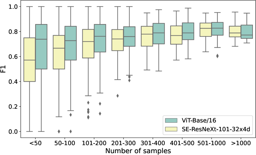
Figure 5: Box plot of the dependence of classification performance ($\text{F}_{1}$) on the number of training samples of a class. Tested on DF20 with input resolution of $224\times 224$.

References

- [1] Suchet Bargoti and James Underwood. Image classification with orchard metadata. In 2016 IEEE International Conference on Robotics and Automation (ICRA), pages 5164–5170. IEEE, 2016.
- [2] Thomas Berg, Jiongxin Liu, Seung Woo Lee, Michelle L. Alexander, David W. Jacobs, and Peter N. Belhumeur. Birdsnap: Large-scale fine-grained visual categorization of birds. 2014 IEEE Conference on Computer Vision and Pattern Recognition, pages 2019–2026, 2014.
- [3] Lucas Beyer, Olivier J Hénaff, Alexander Kolesnikov, Xiaohua Zhai, and Aäron van den Oord. Are we done with imagenet? arXiv preprint arXiv:2006.07159, 2020.
- [4] Steve Branson, Grant Van Horn, Serge Belongie, and Pietro Perona. Bird species categorization using pose normalized deep convolutional nets. arXiv preprint arXiv:1406.2952, 2014.
- [5] Alexander Buslaev, Vladimir I. Iglovikov, Eugene Khvedchenya, Alex Parinov, Mikhail Druzhinin, and Alexandr A. Kalinin. Albumentations: Fast and flexible image augmentations. Information, 11(2), 2020.
- [6] Danish Mycological Society. https://svampe.databasen.org, 2009.
- [7] Jia Deng, Wei Dong, Richard Socher, Li-Jia Li, Kai Li, and Li Fei-Fei. Imagenet: A large-scale hierarchical image database. 2009 IEEE Conference on Computer Vision and Pattern Recognition, pages 248–255, 2009.
- [8] Alexey Dosovitskiy, Lucas Beyer, Alexander Kolesnikov, Dirk Weissenborn, Xiaohua Zhai, Thomas Unterthiner, Mostafa Dehghani, Matthias Minderer, Georg Heigold, Sylvain Gelly, et al. An image is worth 16x16 words: Transformers for image recognition at scale. arXiv preprint arXiv:2010.11929, 2020.
- [9] Jeffrey S Ellen, Casey A Graff, and Mark D Ohman. Improving plankton image classification using context metadata. Limnology and Oceanography: Methods, 17(8):439–461, 2019.
- [10] M. Everingham, L. Van Gool, C. K. I. Williams, J. Winn, and A. Zisserman. The pascal visual object classes (voc) challenge. International Journal of Computer Vision, 88(2):303–338, June 2010.
- [11] Tobias Guldberg Frøslev, Jacob Heilmann-Clausen, Christian Lange, Thomas Læssøe, Jens Henrik Petersen, Ulrik Søchting, Thomas Stjernegaard Jeppesen, and Jan Vesterholt. Danish mycological society, fungal records database, 2019.
- [12] Timnit Gebru, Judy Hoffman, and Li Fei-Fei. Fine-grained recognition in the wild: A multi-task domain adaptation approach. In Proceedings of the IEEE International Conference on Computer Vision, pages 1349–1358, 2017.
- [13] Hervé Goëau, Pierre Bonnet, and Alexis Joly. Plant identification in an open-world (lifeclef 2016). In CLEF working notes 2016, 2016.
- [14] Herve Goeau, Pierre Bonnet, and Alexis Joly. Plant identification based on noisy web data: the amazing performance of deep learning (lifeclef 2017). 2017.
- [15] Wonjoon Goo, Juyong Kim, Gunhee Kim, and Sung Ju Hwang. Taxonomy-regularized semantic deep convolutional neural networks. In European Conference on Computer Vision, pages 86–101. Springer, 2016.
- [16] Chuan Guo, Geoff Pleiss, Yu Sun, and Kilian Q Weinberger. On calibration of modern neural networks. In International Conference on Machine Learning, pages 1321–1330. PMLR, 2017.
- [17] Kaiming He, Haoqi Fan, Yuxin Wu, Saining Xie, and Ross Girshick. Momentum contrast for unsupervised visual representation learning. In Proceedings of the IEEE/CVF Conference on Computer Vision and Pattern Recognition (CVPR), June 2020.
- [18] Kaiming He, Xiangyu Zhang, Shaoqing Ren, and Jian Sun. Deep residual learning for image recognition. In Proceedings of the IEEE conference on computer vision and pattern recognition, pages 770–778, 2016.
- [19] Jacob Heilmann-Clausen, Hans Henrik Bruun, Rasmus Ejrnæs, Tobias Guldberg Frøslev, Thomas Læssøe, and Jens H. Petersen. How citizen science boosted primary knowledge on fungal biodiversity in denmark. Biological Conservation, 237:366 – 372, 2019.
- [20] Saihui Hou, Yushan Feng, and Zilei Wang. Vegfru: A domain-specific dataset for fine-grained visual categorization. In Proceedings of the IEEE International Conference on Computer Vision (ICCV), Oct 2017.
- [21] Jie Hu, Li Shen, and Gang Sun. Squeeze-and-excitation networks. In The IEEE Conference on Computer Vision and Pattern Recognition (CVPR), 2018.
- [22] Alexis Joly, Hervé Goëau, Hervé Glotin, Concetto Spampinato, Pierre Bonnet, Willem-Pier Vellinga, Robert Planqué, Andreas Rauber, Simone Palazzo, Bob Fisher, et al. Lifeclef 2015: multimedia life species identification challenges. In International Conference of the Cross-Language Evaluation Forum for European Languages, pages 462–483. Springer, 2015.
- [23] Aditya Khosla, Nityananda Jayadevaprakash, Bangpeng Yao, and Fei-Fei Li. Novel dataset for fine-grained image categorization : Stanford dogs. 2012.
- [24] Jonathan Krause, Benjamin Sapp, Andrew Howard, Howard Zhou, Alexander Toshev, Tom Duerig, James Philbin, and Li Fei-Fei. The unreasonable effectiveness of noisy data for fine-grained recognition. In European Conference on Computer Vision, pages 301–320. Springer, 2016.
- [25] Jonathan Krause, Michael Stark, Jia Deng, and Fei Fei Li. 3d object representations for fine-grained categorization. 11 2013.
- [26] Alex Krizhevsky. Convolutional deep belief networks on cifar-10, 2010.
- [27] Neeraj Kumar, Peter N. Belhumeur, Arijit Biswas, David W. Jacobs, W. John Kress, Ida Lopez, and João V. B. Soares. Leafsnap: A computer vision system for automatic plant species identification. In The 12th European Conference on Computer Vision (ECCV), October 2012.
- [28] Zhizhong Li and Derek Hoiem. Learning without forgetting. IEEE transactions on pattern analysis and machine intelligence, 40(12):2935–2947, 2017.
- [29] Tsung-Yu Lin, Aruni RoyChowdhury, and Subhransu Maji. Bilinear cnn models for fine-grained visual recognition. In Proceedings of the IEEE international conference on computer vision, pages 1449–1457, 2015.
- [30] Jiongxin Liu, Angjoo Kanazawa, David Jacobs, and Peter Belhumeur. Dog breed classification using part localization. In European conference on computer vision, pages 172–185. Springer, 2012.
- [31] Oisin Mac Aodha, Elijah Cole, and Pietro Perona. Presence-only geographical priors for fine-grained image classification. In Proceedings of the IEEE/CVF International Conference on Computer Vision (ICCV), October 2019.
- [32] S. Maji, J. Kannala, E. Rahtu, M. Blaschko, and A. Vedaldi. Fine-grained visual classification of aircraft. Technical report, 2013.
- [33] Maria-Elena Nilsback and Andrew Zisserman. Automated flower classification over a large number of classes. 2008 Sixth Indian Conference on Computer Vision, Graphics & Image Processing, pages 722–729, 2008.
- [34] Hyun Oh Song, Yu Xiang, Stefanie Jegelka, and Silvio Savarese. Deep metric learning via lifted structured feature embedding. In Proceedings of the IEEE conference on computer vision and pattern recognition, pages 4004–4012, 2016.
- [35] Adam Paszke, Sam Gross, Francisco Massa, Adam Lerer, James Bradbury, Gregory Chanan, Trevor Killeen, Zeming Lin, Natalia Gimelshein, Luca Antiga, Alban Desmaison, Andreas Kopf, Edward Yang, Zachary DeVito, Martin Raison, Alykhan Tejani, Sasank Chilamkurthy, Benoit Steiner, Lu Fang, Junjie Bai, and Soumith Chintala. Pytorch: An imperative style, high-performance deep learning library. In H. Wallach, H. Larochelle, A. Beygelzimer, F. d'Alché-Buc, E. Fox, and R. Garnett, editors, Advances in Neural Information Processing Systems 32, pages 8024–8035. Curran Associates, Inc., 2019.
- [36] Olga Russakovsky, Jia Deng, Hao Su, Jonathan Krause, Sanjeev Satheesh, Sean Ma, Zhiheng Huang, Andrej Karpathy, Aditya Khosla, Michael Bernstein, Alexander C. Berg, and Li Fei-Fei. ImageNet Large Scale Visual Recognition Challenge. International Journal of Computer Vision (IJCV), 115(3):211–252, 2015.
- [37] Mark Sandler, Andrew Howard, Menglong Zhu, Andrey Zhmoginov, and Liang-Chieh Chen. Mobilenetv2: Inverted residuals and linear bottlenecks. In Proceedings of the IEEE Conference on Computer Vision and Pattern Recognition, pages 4510–4520, 2018.
- [38] Kihyuk Sohn. Improved deep metric learning with multi-class n-pair loss objective. In Proceedings of the 30th International Conference on Neural Information Processing Systems, pages 1857–1865, 2016.
- [39] Milan Sulc and Jiri Matas. Improving cnn classifiers by estimating test-time priors. arXiv preprint arXiv:1805.08235v2, 2019.
- [40] Milan Sulc, Lukas Picek, Jiri Matas, Thomas Jeppesen, and Jacob Heilmann-Clausen. Fungi recognition: A practical use case. In Proceedings of the IEEE/CVF Winter Conference on Applications of Computer Vision (WACV), March 2020.
- [41] Christian Szegedy, Sergey Ioffe, Vincent Vanhoucke, and Alexander A Alemi. Inception-v4, inception-resnet and the impact of residual connections on learning. In Thirty-First AAAI Conference on Artificial Intelligence, 2017.
- [42] Faezeh Tafazzoli, Hichem Frigui, and Keishin Nishiyama. A large and diverse dataset for improved vehicle make and model recognition. In Proceedings of the IEEE Conference on Computer Vision and Pattern Recognition Workshops, pages 1–8, 2017.
- [43] Mingxing Tan and Quoc V Le. Efficientnet: Rethinking model scaling for convolutional neural networks. arXiv preprint arXiv:1905.11946, 2019.
- [44] Juozas Vaicenavicius, David Widmann, Carl Andersson, Fredrik Lindsten, Jacob Roll, and Thomas Schön. Evaluating model calibration in classification. In The 22nd International Conference on Artificial Intelligence and Statistics, pages 3459–3467. PMLR, 2019.
- [45] Grant Van Horn, Steve Branson, Ryan Farrell, Scott Haber, Jessie Barry, Panos Ipeirotis, Pietro Perona, and Serge Belongie. Building a bird recognition app and large scale dataset with citizen scientists: The fine print in fine-grained dataset collection. In Proceedings of the IEEE Conference on Computer Vision and Pattern Recognition, pages 595–604, 2015.
- [46] Grant Van Horn, Oisin Mac Aodha, Yang Song, Yin Cui, Chen Sun, Alex Shepard, Hartwig Adam, Pietro Perona, and Serge Belongie. The inaturalist species classification and detection dataset. In Proceedings of the IEEE conference on computer vision and pattern recognition, pages 8769–8778, 2018.
- [47] Ashish Vaswani, Noam Shazeer, Niki Parmar, Jakob Uszkoreit, Llion Jones, Aidan N Gomez, Lukasz Kaiser, and Illia Polosukhin. Attention is all you need. arXiv preprint arXiv:1706.03762, 2017.
- [48] C. Wah, S. Branson, P. Welinder, P. Perona, and S. Belongie. The Caltech-UCSD Birds-200-2011 Dataset. Technical Report CNS-TR-2011-001, California Institute of Technology, 2011.
- [49] Davis Wertheimer and Bharath Hariharan. Few-shot learning with localization in realistic settings. In Proceedings of the IEEE/CVF Conference on Computer Vision and Pattern Recognition, pages 6558–6567, 2019.
- [50] Saining Xie, Ross Girshick, Piotr Dollár, Zhuowen Tu, and Kaiming He. Aggregated residual transformations for deep neural networks. In Proceedings of the IEEE conference on computer vision and pattern recognition, pages 1492–1500, 2017.
- [51] Tao Xu, Pengchuan Zhang, Qiuyuan Huang, Han Zhang, Zhe Gan, Xiaolei Huang, and Xiaodong He. Attngan: Fine-grained text to image generation with attentional generative adversarial networks. In Proceedings of the IEEE conference on computer vision and pattern recognition, pages 1316–1324, 2018.
- [52] Junho Yim, Donggyu Joo, Jihoon Bae, and Junmo Kim. A gift from knowledge distillation: Fast optimization, network minimization and transfer learning. In Proceedings of the IEEE Conference on Computer Vision and Pattern Recognition, pages 4133–4141, 2017.
- [53] Andrew Zhai and Hao-Yu Wu. Classification is a strong baseline for deep metric learning. In Proceedings of the British machine vision conference, 2019.
- [54] Quanshi Zhang, Ying Nian Wu, and Song-Chun Zhu. Interpretable convolutional neural networks. In Proceedings of the IEEE Conference on Computer Vision and Pattern Recognition, pages 8827–8836, 2018.
- [55] Xiaopeng Zhang, Hongkai Xiong, Wengang Zhou, Weiyao Lin, and Qi Tian. Picking deep filter responses for fine-grained image recognition. In Proceedings of the IEEE conference on computer vision and pattern recognition, pages 1134–1142, 2016.
- [56] Zhedong Zheng, Liang Zheng, and Yi Yang. Unlabeled samples generated by gan improve the person re-identification baseline in vitro. In Proceedings of the IEEE International Conference on Computer Vision, pages 3754–3762, 2017.