Relativistic spin sum rules and the role of the pivot

Abstract

Spin sum rules depend on the choice of a pivot, i.e. the point about which the angular momentun is defined, usually identified with the center of the nucleon. The latter is however not unique in a relativistic theory and has led to apparently contradictory results in the literature. Using the recently developed phase-space approach, we compute for the first time the contribution associated with the motion of the center of the nucleon, and we derive a general spin sum rule which reduces to established results after appropriate choices for the pivot and the spin component.

I Introduction

After more than three decades of intense study on both theoretical and experimental sides, the spin structure of the nucleon remains one of the most vivid topics in hadronic physics. Reviews about key developments and achievements in this field can be found in Refs. Filippone:2001ux ; Bass:2004xa ; Aidala:2012mv ; Leader:2013jra ; Wakamatsu:2014zza ; Liu:2015xha ; Deur:2018roz ; Ji:2020ena . A fundamental question is the decomposition of the nucleon spin into its constituents’ intrinsic and orbital angular momentum contributions. While longitudinal spin (or helicity) sum rules derived long ago Jaffe:1989jz ; Ji:1996ek are well-established, various transverse spin sum rules have been discussed over the years and led to a rather confused situation Burkardt:2002hr ; Bakker:2004ib ; Burkardt:2005hp ; Leader:2011cr ; Ji:2012sj ; Ji:2012vj ; Leader:2012md ; Harindranath:2012wn ; Leader:2012ar ; Hatta:2012jm ; Harindranath:2013goa ; Ji:2013tva . Deriving a transverse spin sum rule is a delicate and subtle problem for the simple reason that transverse rotations (unlike longitudinal rotations) do not commute with longitudinal boosts. In the review Leader:2013jra , a whole section has been devoted to discuss in detail these spin sum rules and to clarify their status.

In a recent paper Ji:2020hii a number of results about the transverse angular momentum (AM) in a transversely polarized nucleon are derived, and seem to contradict those obtained earlier in Refs. Bakker:2004ib ; Leader:2011cr . The authors argue that the old results are “incorrect” because they contain, in a moving frame, contributions from the center of mass motion. To get rid of these contributions, they observe that some terms in the expectation value of the transverse AM do not contribute to the Pauli-Lubański pseudovector, and accordingly remove them by hand. This prescription appears however somewhat ad hoc and requires rigorous justification. In particular, the contribution from the center-of-mass motion is actually never calculated.

In this paper, we show that the old Bakker:2004ib ; Leader:2011cr and the new Ji:2020hii results are in fact both correct. They just refer to different definitions for the “center” of the nucleon, and hence for what is meant by “spin” or “internal AM”. The key role played by this center was recognized long ago Bakker:2004ib ; Burkardt:2002hr ; Burkardt:2005hp ; Lorce:2011kn and motivated a recent discussion of the concept of relativistic center of mass in the context of hadronic physics Lorce:2018zpf , which clarified the leading-twist picture of AM in the light-front formalism addressed in Refs. Hoodbhoy:1998yb ; Burkardt:2002hr ; Burkardt:2005hp ; Ji:2012sj ; Ji:2012vj . Here we adopt the phase-space approach developed in Refs. Lorce:2018zpf ; Lorce:2017wkb ; Lorce:2018egm to identify and compute explicitly the contribution from the center-of-mass motion. In the case of the transverse AM, we show that adding this contribution is equivalent to the somewhat ad hoc prescription used in Ref. Ji:2020hii . We observe however that this prescription applies only to the AM operators and leads to incorrect results for the transverse boost operators.

The rest of this paper is organized as follows. In Sec. II we review the notion of spin in Quantum Field Theory and the problem of defining the center of the nucleon. Then we explain in Sec. III how to compute rigorously the expectation values for operators of the form $\int\mathrm{d}^{3}r\,r^{i}O(r)$ and apply the formalism to the Poincaré generators in Sec. IV, followed by a derivation of the general spin sum rule and a comparison with former results found in the literature. Finally, we summarize our findings in Sec. V.

II What do we mean by “spin”?

An AM operator is usually understood as a generator of rotations about some point, the pivot. In practice, once a Lorentz frame is fixed, the origin of the coordinate system is often chosen to coincide with the pivot. But the choice of the pivot is arbitrary. It is in general an abstract concept unless it is given some physical meaning. For example, in the simplest non-relativistic treatment of the hydrogen atom the pivot is placed at the nucleus, which is taken to be an infinitely heavy point charge, with the spinless electron moving in its Coulomb potential.

Problems with understanding the magnetic moment in the Stern-Gerlach experiment led to the introduction of “spin” in Quantum Mechanics to represent some new intrinsic property of the electron, eventually recognized as a new type of AM with no classical analog. The concept of spin was then extended to composite systems and identified with the internal AM, defined as

$$\boldsymbol{S}=\boldsymbol{J}-\boldsymbol{R}\times\boldsymbol{P},$$ (1)

where $\boldsymbol{J}$ is the total AM about the origin, $\boldsymbol{R}$ is the “position” of the system with respect to that origin, and $\boldsymbol{P}$ is its total momentum.

If one requires $\boldsymbol{S}$ to generate internal rotations, i.e. rotations about the position of the system, then the external AM operator $\boldsymbol{L}=\boldsymbol{R}\times\boldsymbol{P}$ must generate external rotations about the origin, i.e. it must satisfy the following commutation relations

$$[R^{i},L^{j}]=i\epsilon^{ijk}R^{k},\qquad[P^{i},L^{j}]=i\epsilon^{ijk}P^{k},$$ (2)

and hence $[L^{i},L^{j}]=i\epsilon^{ijk}L^{k}$. The necessary and sufficient conditions for these to hold are that the operators $\boldsymbol{R}$ and $\boldsymbol{P}$ obey the standard canonical commutation relations

$$[R^{i},R^{j}]=0,\qquad[P^{i},P^{j}]=0,\qquad[R^{i},P^{j}]=i\delta^{ij}.$$ (3)

They imply in particular

$$[R^{i},S^{j}]=0,\qquad[P^{i},S^{j}]=0,\qquad[S^{i},S^{j}]=i\epsilon^{ijk}S^{k}.$$ (4)

In other words, the internal AM operator $\boldsymbol{S}$ satisfies the usual $su(2)$ algebra and is independent of the position and the total momentum of the system, and therefore of the external AM operator $\boldsymbol{L}$.

The question of interest is: what point defines the position of the system? In non-relativistic Quantum Mechanics, it is defined by the center-of-mass position operator

$$\boldsymbol{R}:=\boldsymbol{R}_{\text{NR}}=\frac{1}{m}\sum_{n=1}^{N}m_{n}\boldsymbol{R}_{n},$$ (5)

where $m=\sum_{n}m_{n}$ is the mass of a system made of $N$ particles with masses $m_{n}$. Since the particles’ position and momentum operators satisfy by definition $[R^{i}_{n},P^{j}_{n^{\prime}}]=i\delta^{ij}\delta_{nn^{\prime}}$ with $[R^{i}_{n},R^{j}_{n^{\prime}}]=0$ and $[P^{i}_{n},P^{j}_{n^{\prime}}]=0$, one sees that the non-relativistic spin operator $\boldsymbol{S}_{\text{NR}}=\boldsymbol{J}-\boldsymbol{R}_{\text{NR}}\times\boldsymbol{P}$ is the generator of internal rotations. If the system consists of a single structureless particle, then the non-relativistic spin operator simply coincides with the intrinsic AM operator.

In a relativistic theory, the situation is more complicated for two reasons:

• There exist different expressions for the AM operators in terms of the fields associated with the particles. The two principal versions are the Canonical and the Belinfante (or symmetrized) forms, which differ by a spatial integral over fields evaluated at infinity. As explained in Section 2.6.3 of Ref. Leader:2013jra , it would be impossible to construct a consistent theory if one could not ignore such terms in the matrix elements of these AM operators taken between normalizable states. Hence we may choose which version to use, and in this paper, as is done in the papers we are commenting on, we shall only use the Belinfante versions.

• In particle physics it is often adequate to describe the motion of a particle as being in a momentum eigenstate, i.e. a plane wave, but clearly in that case the density in coordinate space is constant so that the particle is totally delocalized. So, to discuss internal AM some form of localized wave packet is essential. In addition, even when dealing with a localized system, there still exist several possibilities for the definition of the position of the system, which are identical in the rest frame of the system, but generally differ in other frames. The main three definitions are given by the so-called relativistic centers of energy (or inertia), mass, and spin Pryce:1948pf ; Moller:1949 ; Fleming:1965 ; Choi:2014nea ; Lorce:2018zpf , which we briefly review in the following.

II.1 The relativistic center of energy or inertia

The relativistic center of energy or inertia is the field theoretical version of Eq. (5), where the role of inertial mass is played by the energy. Its position and time component are defined, in any reference frame, by Fokker:1929 ; Born:1935ap

$$R^{\mu}_{E}=\frac{1}{P^{0}}\int\mathrm{d}^{3}r\,r^{\mu}\,T^{00}(r),$$ (6)

where the operator $T^{\mu\nu}(r)$ is the energy momentum tensor (EMT) and $P^{\mu}=\int\mathrm{d}^{3}r\,T^{0\mu}(r)$ is the total four-momentum operator. Acting on a four-momentum eigenstate with eigenvalue $p^{\mu}$, the operator $1/P^{0}$ simply means multiplication by $1/p^{0}$. Also, ambiguities in the ordering of Hermitian operators are resolved by considering implicitly symmetrized products $AB\equiv\frac{1}{2}(AB+BA)$ Born:1935ap ; Pryce:1948pf .

In a field theory, the AM generators $J^{i}=\frac{1}{2}\epsilon^{ijk}M^{jk}$ and the generators of boosts $K^{i}=M^{0i}$ are defined in terms of the generalized AM momentum tensor, which reads in Belinfante form Belinfante:1940

$$M^{\mu\nu}=-M^{\nu\mu}=\int\mathrm{d}^{3}r\left[r^{\mu}T^{0\nu}(r)-r^{\nu}T^{0\mu}(r)\right].$$ (7)

It follows that the position operator for the relativistic center of energy is directly related to the generators of boosts as follows

$$\boldsymbol{R}_{E}=t\,\frac{\boldsymbol{P}}{P^{0}}-\frac{\boldsymbol{K}}{P^{0}}.$$ (8)

Clearly, $R^{\mu}_{E}$ does not transform as a Lorentz four-vector. Using the following commutation relations

$$[K^{i},K^{j}]=-i\epsilon^{ijk}J^{k},\qquad[P^{0},K^{i}]=iP^{i},\qquad[P^{i},K^{j}]=i\delta^{ij}P^{0},$$ (9)

and the fact that $\boldsymbol{J}$ generates the rotations, one can check that $\boldsymbol{R}_{E}$ satisfies the canonical commutation relations $[R^{i}_{E},P^{j}]=i\delta^{ij}$ and $[R^{i}_{E},J^{j}]=i\epsilon^{ijk}R^{k}_{E}$, so that it qualifies to some extent as a position operator, albeit with mutually non-commuting components. This last property implies that $\boldsymbol{R}_{E}\times\boldsymbol{P}$ will not satisfy the $su(2)$ algebra and cannot be considered as a genuine orbital AM operator. Nonetheless, as is customary, we shall continue to refer to it as the AM of the center of energy about the origin.

The nearest one can get to a spin operator transforming as a four-vector is the Pauli-Lubański pseudovector Lubanski:1942 ; Lubanski:1942bis

$$W^{\mu}=\frac{1}{2}\,\epsilon^{\mu\alpha\beta\lambda}M_{\alpha\beta}P_{\lambda},$$ (10)

which satisfies the commutation relations

$$[W^{\mu},P^{\nu}]=0,\qquad[W^{\mu},W^{\nu}]=-\epsilon^{\mu\nu\alpha\beta}W_{\alpha}P_{\beta}$$ (11)

in the convention $\epsilon_{0123}=1$. For a momentum eigenstate with $\boldsymbol{p}=\boldsymbol{0}$, the action of $\boldsymbol{W}$ coincides with that of $m\boldsymbol{J}$. Hence one can define a relativistic spin operator by

$$\boldsymbol{S}_{E}=\frac{\boldsymbol{W}}{P^{0}}=\boldsymbol{J}+\frac{\boldsymbol{K}\times\boldsymbol{P}}{P^{0}}=\boldsymbol{J}-\boldsymbol{R}_{E}\times\boldsymbol{P},$$ (12)

showing that $\boldsymbol{S}_{E}$ corresponds to the internal AM about the relativistic center of energy. Note however that, like the external AM $\boldsymbol{R}_{E}\times\boldsymbol{P}$, it is not a genuine AM operator. An explicit calculation gives indeed Born:1935ap ; Pryce:1948pf

$$[S^{i}_{E},S^{j}_{E}]=i\epsilon^{ijk}\left(\delta^{kl}-\frac{P^{k}P^{l}}{(P^{0})^{2}}\right)S_{E}^{l}$$ (13)

and shows that $\boldsymbol{S}_{E}$ does not obey the $su(2)$ algebra, except when acting on a momentum eigenstate with $\boldsymbol{p}=\boldsymbol{0}$.

II.2 The relativistic center of mass

As already mentioned, the relativistic center of energy $\boldsymbol{R}_{E}$ does not behave as the spatial part of a Lorentz four-vector. This is not a fundamental issue since the center of a system is just a representative point to which one can attach global properties like mass, momentum and spin. It does not need to behave as an actual physical point. As a result, different observers will generally locate the center of energy at different places inside the convex hull of the system Moller:1949 ; Moller:1949bis . One may then wonder whether it is possible to define a natural relativistic center whose coordinates would transform as part of a Lorentz four-vector.

Clearly, the center of energy defined in the rest frame of the system plays a special role. Since in that frame the energy coincides with the mass of the system, we will refer to it as the relativistic center of mass. At the classical level, if $r^{\mu}_{E}|_{\text{rest}}$ represents the space-time coordinates of the relativistic center of mass in the rest frame, its components in an arbitrary frame will be defined by $r^{\mu}_{M}=\Lambda^{\mu}_{\phantom{\mu}\nu}r^{\nu}_{E}|_{\text{rest}}$, where $\Lambda^{\mu}_{\phantom{\mu}\nu}$ represents the Lorentz transformation from the rest frame to the moving frame, i.e. such that $p^{\mu}=\Lambda^{\mu}_{\phantom{\mu}\nu}p^{\nu}_{\text{rest}}$ with $p^{\mu}_{\text{rest}}=(m,\boldsymbol{0})$. Transposing this construction to an operator level is not so trivial. First, one needs to clarify what is meant by “a system at rest” in a quantum theory. Since $\boldsymbol{P}$ is an operator, the rest frame will simply mean the frame in which the expectation value of the total momentum operator vanishes

$$\langle\boldsymbol{P}\rangle|_{\text{rest}}=\boldsymbol{0}.$$ (14)

Second, since $R^{\mu}_{E}$ involves symmetrized products of operators, the above classical requirements are transposed in a quantum theory into requirements on the expectation values, namely

$$\langle R^{\mu}_{M}\rangle=\Lambda^{\mu}_{\phantom{\mu}\nu}\langle R^{\nu}_{E}\rangle|_{\text{rest}},\qquad\langle P^{\mu}\rangle=\Lambda^{\mu}_{\phantom{\mu}\nu}\langle P^{\nu}\rangle|_{\text{rest}}.$$ (15)

A manifestly covariant generalization of Eq. (8) is given by Pryce:1948pf ; Fleming:1965

$$R_{\star}^{\mu}=\tau\,\frac{P^{\mu}}{M}-\frac{P_{\nu}M^{\nu\mu}}{M^{2}},$$ (16)

where $\tau$ is the proper time, $P_{\nu}M^{\nu\mu}/M$ is the covariant form of the boost generators defined by a comoving observer, and $M=\sqrt{P^{2}}$ is the mass operator. In the rest frame, proper time coincides with the time coordinate so that one has as required $\langle R^{\mu}_{\star}\rangle|_{\text{rest}}=\langle R^{\mu}_{E}\rangle|_{\text{rest}}$. The only problems are that $[R^{i}_{\star},P^{j}]=i\left(\delta^{ij}+\frac{P^{i}P^{j}}{M^{2}}\right)$ and $R^{0}_{\star}\neq t$, and have to do with the fact that the operator $\boldsymbol{R}_{\star}$ represents a position at a fixed proper time $\tau$ and not at a fixed time coordinate $t$. The solution is to use another operator Pryce:1948pf ; Fleming:1965

$$R_{M}^{\mu}=\left(t+\frac{\boldsymbol{P}\cdot\boldsymbol{K}}{M^{2}}\right)\frac{P^{\mu}}{P^{0}}-\frac{P_{\nu}M^{\nu\mu}}{M^{2}}$$ (17)

that satisfies $[R^{i}_{M},P^{j}]=i\delta^{ij}$ and $R^{0}_{M}=t$. Despite its lack of manifest covariance, it describes in any frame the same world line as $R^{\mu}_{\star}$, namely

$$\{\langle R^{\mu}_{M}\rangle\,|\,t\in\text{Reals}\}=\{\langle R^{\mu}_{\star}\rangle\,|\,\tau\in\text{Reals}\}.$$ (18)

In other words, the expectation value $\langle R^{\mu}_{M}\rangle$ transforms as a Lorentz four-vector. Moreover, one has obviously $\langle R^{\mu}_{M}\rangle|_{\text{rest}}=\langle R^{\mu}_{E}\rangle|_{\text{rest}}$.

Combining Eqs. (17) and (8), one finds that the shift between the relativistic centers of energy and mass is given by

$$\boldsymbol{R}_{E}-\boldsymbol{R}_{M}=\frac{\boldsymbol{P}\times\boldsymbol{W}}{P^{0}M^{2}}.$$ (19)

The internal AM operator about the relativistic center of mass $\boldsymbol{S}_{M}=\boldsymbol{J}-\boldsymbol{R}_{M}\times\boldsymbol{P}$ can then be expressed in terms of the Pauli-Lubański pseudovector as follows

$$\boldsymbol{S}_{M}=\frac{P^{0}\boldsymbol{W}-\boldsymbol{P}W^{0}}{M^{2}}.$$ (20)

Under Lorentz transformations, it behaves in the same way as the total AM $\boldsymbol{J}$, i.e. as the axial-vector part $S^{i}_{M}=\frac{1}{2}\,\epsilon^{ijk}S^{jk}_{M}$ of a rank-two antisymmetric Lorentz tensor $S^{\mu\nu}_{M}=-\epsilon^{\mu\nu\rho\sigma}W_{\rho}P_{\sigma}/M^{2}$. Note however that, like $\boldsymbol{R}_{E}$, the components of $\boldsymbol{R}_{M}$ do not commute with each other. It is also easy to check that $\boldsymbol{S}_{M}$ does not satisfy the $su(2)$ algebra Pryce:1948pf

$$[S^{i}_{M},S^{j}_{M}]=i\epsilon^{ijk}\left(\delta^{kl}+\frac{P^{k}P^{l}}{M^{2}}\right)S_{M}^{l}$$ (21)

and cannot be considered as a genuine AM operator, except when acting on a momentum eigenstate with $\boldsymbol{p}=\boldsymbol{0}$.

II.3 The relativistic center of spin

As stressed above, neither the components of $\boldsymbol{R}_{E}$ nor those of $\boldsymbol{R}_{M}$ commute with each other Born:1935ap ; Pryce:1948pf ; Moller:1949 ; Fleming:1965 . The corresponding spin operators $\boldsymbol{S}_{E}$ and $\boldsymbol{S}_{M}$ do not satisfy the $su(2)$ algebra of AM operators, and hence cannot be considered as generators of rotations. Remarkably, it has been observed that a position operator with commuting components can be obtained by an appropriate weighted average of $R^{\mu}_{E}$ and $R^{\mu}_{M}$ Pryce:1935ibt ; Pryce:1948pf ; Moller:1949

$$R^{\mu}_{c}=\frac{P^{0}R^{\mu}_{E}+MR^{\mu}_{M}}{P^{0}+M},$$ (22)

proved to be unique by Newton and Wigner Newton:1949cq . Clearly, like $\boldsymbol{R}_{E}$ and $\boldsymbol{R}_{M}$, the operator $\boldsymbol{R}_{c}$ satisfies the commutations relations $[R^{i}_{c},P^{j}]=i\delta^{ij}$ and $[R^{i}_{c},J^{j}]=i\epsilon^{ijk}R^{k}_{c}$, and therefore qualifies as a position operator.

The corresponding internal AM operator $\boldsymbol{S}_{c}=\boldsymbol{J}-\boldsymbol{R}_{c}\times\boldsymbol{P}$ reads Pryce:1935ibt ; Pryce:1948pf ; Moller:1949 ; Bogolyubov:1975ps ; Choi:2014nea

$$\boldsymbol{S}_{c}=\frac{P^{0}\boldsymbol{S}_{E}+M\boldsymbol{S}_{M}}{P^{0}+M}=\frac{\boldsymbol{W}}{M}-\frac{\boldsymbol{P}W^{0}}{M(P^{0}+M)}.$$ (23)

It satisfies the familiar commutation relations

$$[S^{i}_{c},S^{j}_{c}]=i\epsilon^{ijk}S^{k}_{c},\qquad[S^{i}_{c},R^{j}_{c}]=0,\qquad[S^{i}_{c},P^{j}]=0,$$ (24)

and can therefore be interpreted as the generator of internal rotations. For these reasons, the point located at $\langle\boldsymbol{R}_{c}\rangle$ has been called the relativistic center of spin in Refs. Fleming:1965 ; Schwartz:2020lys and the canonical reference point in Ref. Lorce:2018zpf .

Since $P\cdot W=0$, the canonical spin operator can be put in the form Keister:1991sb

$$S^{\mu}_{c}=(L^{-1}_{c}(P))^{\mu}_{\phantom{\mu}\nu}\,\frac{W^{\nu}}{M}$$ (25)

with $S^{0}_{c}=0$. The operator

$$(L^{-1}_{c}(P))^{\mu}_{\phantom{\mu}\nu}=\delta^{\mu}_{\nu}-\frac{(P^{\mu}+M\delta^{\mu}_{0})(P_{\nu}+M\delta^{0}_{\nu})}{M(P^{0}+M)}+2\frac{\delta^{\mu}_{0}P_{\nu}}{M}$$ (26)

satisfies the properties

$$(L^{-1}_{c}(P))^{\mu}_{\phantom{\mu}\nu}P^{\nu}=M\delta^{\mu}_{0},\qquad P_{\nu}=M\delta^{0}_{\mu}\,(L^{-1}_{c}(P))^{\mu}_{\phantom{\mu}\nu}=(L_{c}(P))_{\nu}^{\phantom{\nu}\mu}M\delta^{0}_{\mu},$$ (27)

and can be understood as the operator analog of $(L^{-1}_{c}(p))^{\mu}_{\phantom{\mu}\nu}$, the canonical (rotationless) four-vector boost from the moving frame to the rest frame Krause:1977yr ; Fahnline:1982 . Sandwiching Eq. (25) between momentum eigenstates, one gets

$$\langle p|S^{i}_{c}|p\rangle =\frac{1}{m}\,(L^{-1}_{c}(p))^{i}_{\phantom{i}\nu}\langle p|W^{\nu}|p\rangle$$ (28)

$$=\frac{1}{m}\,\langle p|U^{-1}(L^{-1}_{c}(p))W^{i}U(L^{-1}_{c}(p))|p\rangle$$

$$=\langle p_{\text{rest}}|J^{i}|p_{\text{rest}}\rangle.$$

Since momentum eigenstates are covariantly normalized, one can write $\langle p|p\rangle=\langle p_{\text{rest}}|p_{\text{rest}}\rangle$ and therefore conclude that the expectation value of canonical spin in an arbitrary frame gives the same value as the rest-frame AM

$$\frac{\langle p|S^{i}_{c}|p\rangle}{\langle p|p\rangle}=\frac{\langle p_{\text{rest}}|J^{i}|p_{\text{rest}}\rangle}{\langle p_{\text{rest}}|p_{\text{rest}}\rangle}.$$ (29)

In particular, a spin-$1/2$ momentum eigenstate with canonical polarization described by the unit vector $\boldsymbol{s}$ is an eigenstate of the canonical spin component along $\boldsymbol{s}$

$$\boldsymbol{s}\cdot\boldsymbol{S}_{c}|p,\boldsymbol{s}\rangle=-\frac{\mathcal{S}_{\mu}W^{\mu}}{m}|p,\boldsymbol{s}\rangle=\tfrac{1}{2}\,|p,\boldsymbol{s}\rangle,$$ (30)

where the (canonical) covariant polarization vector is defined as

$$\mathcal{S}^{\mu}(p,\boldsymbol{s})=(L_{c}(p))^{\mu}_{\phantom{\mu}\nu}\mathcal{S}^{\nu}_{\text{rest}}=\left(\frac{\boldsymbol{p}\cdot\boldsymbol{s}}{m},\boldsymbol{s}+\frac{\boldsymbol{p}(\boldsymbol{p}\cdot\boldsymbol{s})}{m(p^{0}+m)}\right)$$ (31)

with $\mathcal{S}^{\mu}_{\text{rest}}=(0,\boldsymbol{s})$.

As a final remark, it is interesting to express the generators of boosts in terms of the canonical position and spin operators

$$\boldsymbol{K}=\boldsymbol{P}t-P^{0}\boldsymbol{R}_{c}-\frac{\boldsymbol{P}\times\boldsymbol{S}_{c}}{P^{0}+M}.$$ (32)

This relation clearly shows that the operators $\boldsymbol{K}$ generate not only boosts of the system (first two terms), but also rotations in internal or spin space (last term) known as the Wigner rotations Wigner:1939cj ; Polyzou:2012ut , which are responsible for the non-commutativity of the components of $\boldsymbol{K}$.

III Expectation values

Now that the notion of spin and the question of the pivot have been reviewed, we turn our attention to the computation of the expectation values of the Lorentz generators. They require particular care because matrix elements of the type $\langle p,\boldsymbol{s}|\int\mathrm{d}^{3}r\,r^{i}O(r)|p,\boldsymbol{s}\rangle$ are usually ill-defined, being either infinite or, by symmetry, zero. We present in the following the two approaches designed to deal with this problem.

We will always work with covariantly normalized momentum eigenstates $\langle p_{f},\boldsymbol{s}|p_{i},\boldsymbol{s}\rangle=(2\pi)^{3}\,2p^{0}_{i}\,\delta^{(3)}(\boldsymbol{p}_{f}-\boldsymbol{p}_{i})$, so that the completeness relation (resolution of the identity) becomes

$$I=\sum_{\sigma=\pm}\int\frac{\mathrm{d}^{3}p}{(2\pi)^{3}2p_{0}}\,|p,\sigma\boldsymbol{s}\rangle\langle p,\sigma\boldsymbol{s}|.$$ (33)

For later convenience, we introduce the average four-momentum and four-momentum transfer variables

$$\bar{p}=\tfrac{1}{2}(p_{f}+p_{i}),\qquad\Delta=p_{f}-p_{i}$$ (34)

which obey the constraints

$$\bar{p}\cdot\Delta=0,\qquad\bar{p}^{2}=m^{2}-\frac{\Delta^{2}}{4}$$ (35)

owing to the onshell relations $p^{2}_{i}=p^{2}_{f}=m^{2}$.

III.1 Standard approach

The standard approach is a prescription which consists in considering first the matrix element with nonzero momentum transfer $\boldsymbol{\Delta}$, and then taking the forward limit $\boldsymbol{\Delta}\to\boldsymbol{0}$ at the end of the calculation Jaffe:1989jz ; Shore:1999be ; Bakker:2004ib ; Leader:2013jra ; Lowdon:2017idv ; Cotogno:2019xcl ; Lorce:2019sbq

$$\langle p,\boldsymbol{s}|\int\mathrm{d}^{3}r\,r^{i}O(r)|p,\boldsymbol{s}\rangle\equiv\lim_{\boldsymbol{\Delta}\to\boldsymbol{0}}\langle\bar{p}+\tfrac{\Delta}{2},\boldsymbol{s}|\int\mathrm{d}^{3}r\,r^{i}O(r)|\bar{p}-\tfrac{\Delta}{2},\boldsymbol{s}\rangle.$$ (36)

Note that $\bar{\boldsymbol{p}}$ is kept fixed so that $\bar{\boldsymbol{p}}=\boldsymbol{p}$, and from Eq. (35)

$$\bar{p}^{0}=\frac{1}{2}\left(\sqrt{(\boldsymbol{p}+\tfrac{\boldsymbol{\Delta}}{2})^{2}+m^{2}}+\sqrt{(\boldsymbol{p}-\tfrac{\boldsymbol{\Delta}}{2})^{2}+m^{2}}\right)$$ (37)

whereas $p^{0}=\sqrt{\boldsymbol{p}^{2}+m^{2}}$.

For convenience, we will also work at $t=0$ in the following. One can write using translation symmetry and the Leibniz rule

$$\langle\bar{p}+\tfrac{\Delta}{2},\boldsymbol{s}| \int\mathrm{d}^{3}r\,r^{i}O(r)|\bar{p}-\tfrac{\Delta}{2},\boldsymbol{s}\rangle$$ (38)

$$=\int\mathrm{d}^{3}r\,e^{-i\boldsymbol{\Delta}\cdot\boldsymbol{r}}r^{i}\langle\bar{p}+\tfrac{\Delta}{2},\boldsymbol{s}|O(0)|\bar{p}-\tfrac{\Delta}{2},\boldsymbol{s}\rangle$$

$$=\left[(2\pi)^{3}i\nabla^{i}\delta^{(3)}(\boldsymbol{\Delta})\right]\langle\bar{p}+\tfrac{\Delta}{2},\boldsymbol{s}|O(0)|\bar{p}-\tfrac{\Delta}{2},\boldsymbol{s}\rangle$$

$$=i\nabla^{i}\!\left[(2\pi)^{3}\delta^{(3)}(\boldsymbol{\Delta})\,\langle\bar{p}+\tfrac{\Delta}{2},\boldsymbol{s}|O(0)|\bar{p}-\tfrac{\Delta}{2},\boldsymbol{s}\rangle\right]-\left[i\nabla^{i}\langle\bar{p}+\tfrac{\Delta}{2},\boldsymbol{s}|O(0)|\bar{p}-\tfrac{\Delta}{2},\boldsymbol{s}\rangle\right](2\pi)^{3}\delta^{(3)}(\boldsymbol{\Delta})$$

$$=\langle p,\boldsymbol{s}|O(0)|p,\boldsymbol{s}\rangle\,(2\pi)^{3}i\nabla^{i}\delta^{(3)}(\boldsymbol{\Delta})+\left[-i\nabla^{i}\langle\bar{p}+\tfrac{\Delta}{2},\boldsymbol{s}|O(0)|\bar{p}-\tfrac{\Delta}{2},\boldsymbol{s}\rangle\right]_{\boldsymbol{\Delta}=\boldsymbol{0}}(2\pi)^{3}\delta^{(3)}(\boldsymbol{\Delta}),$$

where $\nabla^{i}=\frac{\partial}{\partial\Delta^{i}}$. One then finds for the expectation value

$$\frac{\langle p,\boldsymbol{s}|\int\mathrm{d}^{3}r\,r^{i}O(r)|p,\boldsymbol{s}\rangle}{\langle p,\boldsymbol{s}|p,\boldsymbol{s}\rangle}=\frac{\langle p,\boldsymbol{s}|O(0)|p,\boldsymbol{s}\rangle}{\langle p,\boldsymbol{s}|p,\boldsymbol{s}\rangle}\,(2\pi)^{3}i\nabla^{i}\delta^{(3)}(\boldsymbol{0})+\frac{1}{2p^{0}}\left[-i\nabla^{i}\langle\bar{p}+\tfrac{\Delta}{2},\boldsymbol{s}|O(0)|\bar{p}-\tfrac{\Delta}{2},\boldsymbol{s}\rangle\right]_{\boldsymbol{\Delta}=\boldsymbol{0}}.$$ (39)

Note that in the second term one should not forget that both $\Delta^{0}$ and $\bar{p}^{0}$ are understood as functions of $\boldsymbol{\Delta}$, derived from the onshell constraints (35).

In order to make sense of the highly divergent term in Eq. (39), one has to work with normalizable states and hence introduce some wave packet. Calculations with explicit forms for the wave packets are pretty lengthy and cumbersome, but they show that the highly divergent term corresponds actually to the contribution from the center of the wave packet Jaffe:1989jz ; Bakker:2004ib . Since one is interested in the internal structure of the nucleon and not in the details of the wave packet, this term is usually discarded.

III.2 Phase-space approach

Discarding the highly divergent term in Eq. (39) is tantamount to throwing the baby out with the bathwater. Indeed, even though we are not interested in the details of the wave packet, it is important to retain the information about the position of its center. This can easily be achieved within the phase-space approach developed in Refs. Lorce:2018zpf ; Lorce:2017wkb ; Lorce:2018egm , and used in Ref. Lorce:2020onh to elucidate the momentum dependence of relativistic charge distributions.

In a quantum theory, states localized around the position $\boldsymbol{r}$ at time $t=0$ are defined as the following Fourier transform of momentum eigenstates

$$|\boldsymbol{r}\rangle\equiv\int\frac{\mathrm{d}^{3}p}{(2\pi)^{3}\sqrt{2p^{0}}}\,e^{-i\boldsymbol{p}\cdot\boldsymbol{r}}\,|p\rangle$$ (40)

and are normalized as $\langle\boldsymbol{r}_{f}|\boldsymbol{r}_{i}\rangle=\delta^{(3)}(\boldsymbol{r}_{f}-\boldsymbol{r}_{i})$. Wave packets associated with physical states normalized as $\langle\psi|\psi\rangle=1$ are then defined by

$$\tilde{\psi}(\boldsymbol{p})\equiv\frac{\langle p|\psi\rangle}{\sqrt{2p^{0}}}\qquad\text{so that}\qquad\psi(\boldsymbol{r})\equiv\langle\boldsymbol{r}|\psi\rangle=\int\frac{\mathrm{d}^{3}p}{(2\pi)^{3}}\,e^{i\boldsymbol{p}\cdot\boldsymbol{r}}\,\tilde{\psi}(\boldsymbol{p}).$$ (41)

A physical state cannot be simultaneously in an eigenstate of both position and momentum. But it was shown long ago how to define a quantity, analogous to a density matrix, which gives the quantum weight that a system in a definite state $|\psi\rangle$ will be found to have average position $\boldsymbol{\mathcal{R}}$ and average momentum $\boldsymbol{p}$. This quantum phase-space or Wigner distribution is given by Wigner:1932eb ; Hillery:1983ms

$$\rho_{\psi}(\boldsymbol{\mathcal{R}},\boldsymbol{p}) \equiv\int\mathrm{d}^{3}z\,e^{-i\boldsymbol{p}\cdot\boldsymbol{z}}\,\psi^{*}(\boldsymbol{\mathcal{R}}-\tfrac{\boldsymbol{z}}{2})\psi(\boldsymbol{\mathcal{R}}+\tfrac{\boldsymbol{z}}{2})$$ (42)

$$=\int\frac{\mathrm{d}^{3}q}{(2\pi)^{3}}\,e^{-i\boldsymbol{q}\cdot\boldsymbol{\mathcal{R}}}\,\tilde{\psi}^{*}(\boldsymbol{p}+\tfrac{\boldsymbol{q}}{2})\tilde{\psi}(\boldsymbol{p}-\tfrac{\boldsymbol{q}}{2})$$

and is not positive-definite because of the Heisenberg uncertainty relations. It is thus a quasi-probabilistic density matrix. It can be seen that $\boldsymbol{\mathcal{R}}$ is the average of the initial and final position vectors and $\boldsymbol{p}$ is the average of the initial and final momenta, respectively, in Eq. (42). One recovers a probabilistic interpretation after integration over either average position or average momentum

$$\int\mathrm{d}^{3}\mathcal{R}\,\rho_{\psi}(\boldsymbol{\mathcal{R}},\boldsymbol{p})=|\tilde{\psi}(\boldsymbol{p})|^{2},\qquad\int\frac{\mathrm{d}^{3}p}{(2\pi)^{3}}\,\rho_{\psi}(\boldsymbol{\mathcal{R}},\boldsymbol{p})=|\psi(\boldsymbol{\mathcal{R}})|^{2}.$$ (43)

One can now express the expectation of any operator $O$ as a phase-space integral Wigner:1932eb ; Hillery:1983ms over $\boldsymbol{\mathcal{R}}$ and $\boldsymbol{p}$ of the Wigner distribution times the expectation value of $O$ in a state having average position $\boldsymbol{\mathcal{R}}$ and average momentum $\boldsymbol{p}$, namely

$$\langle\psi|O|\psi\rangle=\int\frac{\mathrm{d}^{3}p}{(2\pi)^{3}}\,\mathrm{d}^{3}\mathcal{R}\,\rho_{\psi}(\boldsymbol{\mathcal{R}},\boldsymbol{p})\,\langle O\rangle_{\boldsymbol{\mathcal{R}},\boldsymbol{p}},$$ (44)

where

$$\langle O\rangle_{\boldsymbol{\mathcal{R}},\boldsymbol{p}}=\int\frac{\mathrm{d}^{3}\Delta}{(2\pi)^{3}}\,e^{i\boldsymbol{\Delta}\cdot\boldsymbol{\mathcal{R}}}\,\frac{\langle\bar{p}+\tfrac{\Delta}{2}|O|\bar{p}-\tfrac{\Delta}{2}\rangle}{\sqrt{4\left(\bar{p}^{0}\right)^{2}-\left(\Delta^{0}\right)^{2}}}\qquad\textrm{with}\qquad\bar{\boldsymbol{p}}=\boldsymbol{p}.$$ (45)

Although originally developed in the non-relativistic context, this formalism carries over to Quantum Field Theory BialynickiBirula:1991tx . Requiring the localization of a system simultaneously in the three spatial dimensions leads automatically to a position operator with mutually commuting components, i.e. to $\boldsymbol{R}_{c}$ which, as mentioned, is the only relativistic operator with that property Pryce:1948pf ; Newton:1949cq ; Foldy:1949wa . It has indeed been shown in Refs. Newton:1949cq ; Pavsic:2017orp that the states $|\boldsymbol{r}\rangle$ defined by Eq. (40) are eigenstates of the canonical position operator

$$\boldsymbol{R}_{c}|\boldsymbol{r}\rangle=\boldsymbol{r}|\boldsymbol{r}\rangle.$$ (46)

Since wave-packet details are encoded in $\rho_{\psi}(\boldsymbol{\mathcal{R}},\boldsymbol{p})$ in Eq. (44), one can interpret $\langle O\rangle_{\boldsymbol{\mathcal{R}},\boldsymbol{p}}$ as the part associated with the internal structure of the system localized in the Wigner sense around the (average) canonical position $\langle\boldsymbol{R}_{c}\rangle_{\boldsymbol{\mathcal{R}},\boldsymbol{p}}=\boldsymbol{\mathcal{R}}$ with (average) momentum $\langle\boldsymbol{P}\rangle_{\boldsymbol{\mathcal{R}},\boldsymbol{p}}=\boldsymbol{p}$. As noted in Ref. Lorce:2018zpf , the standard expectation value (36) corresponds simply to an average over $\boldsymbol{\mathcal{R}}$ of the phase-space expectation value (45)

$$\int\frac{\mathrm{d}^{3}\mathcal{R}}{(2\pi)^{3}\delta^{(3)}(\boldsymbol{0})}\,\langle O\rangle_{\boldsymbol{\mathcal{R}},\boldsymbol{p}}=\int\mathrm{d}^{3}\Delta\,\delta^{(3)}(\boldsymbol{\Delta})\,\frac{\langle\bar{p}+\tfrac{\Delta}{2}|O|\bar{p}-\tfrac{\Delta}{2}\rangle}{(2\pi)^{3}2p^{0}\delta^{(3)}(\boldsymbol{0})}=\frac{\langle p|O|p\rangle}{\langle p|p\rangle}.$$ (47)

Proceeding similarly to Eq. (38), one finds including now polarization Lorce:2018zpf

$$\langle\int\mathrm{d}^{3}r\,r^{i}O(r)\rangle_{\boldsymbol{\mathcal{R}},\boldsymbol{p},\boldsymbol{s}}=\mathcal{R}^{i}\,\frac{\langle p,\boldsymbol{s}|O(0)|p,\boldsymbol{s}\rangle}{2p^{0}}+\frac{1}{2p^{0}}\left[-i\nabla^{i}\langle\bar{p}+\tfrac{\Delta}{2},\boldsymbol{s}|O(0)|\bar{p}-\tfrac{\Delta}{2},\boldsymbol{s}\rangle\right]_{\boldsymbol{\Delta}=\boldsymbol{0}}.$$ (48)

Comparing with Eq. (39), one observes that the highly divergent term is replaced by a well-defined expression in the phase-space approach, which confirms its interpretation as the contribution associated with the center of the wave packet. According to Eq. (47) one should recover Eq. (39) from an average of Eq. (48) over $\boldsymbol{\mathcal{R}}$. Indeed, the second term in Eq. (48) is independent of $\boldsymbol{\mathcal{R}}$ and is therefore not affected by the average over $\boldsymbol{\mathcal{R}}$. The first term however is linear in $\boldsymbol{\mathcal{R}}$ and gives the ambiguous contribution in Eq. (39), since one can formally write $\int\mathrm{d}^{3}\mathcal{R}\,\mathcal{R}^{i}=\lim_{\boldsymbol{\Delta}\to\boldsymbol{0}}\int\mathrm{d}^{3}\mathcal{R}\,e^{-i\boldsymbol{\Delta}\cdot\boldsymbol{\mathcal{R}}}\mathcal{R}^{i}=(2\pi)^{3}\,i\nabla^{i}\delta^{(3)}(\boldsymbol{0})$.

As mentioned earlier, in the literature one is usually interested in the internal part and accordingly considers only the second term in Eq. (48) or Eq. (39) Jaffe:1989jz ; Shore:1999be ; Bakker:2004ib ; Leader:2013jra . This can be justified by choosing the (average) relativistic center of spin as the origin of the coordinate system, i.e. by setting $\boldsymbol{\mathcal{R}}=\boldsymbol{0}$

$$\langle\int\mathrm{d}^{3}r\,r^{i}O(r)\rangle_{\boldsymbol{0},\boldsymbol{p},\boldsymbol{s}}=\frac{1}{2p^{0}}\left[-i\nabla^{i}\langle\bar{p}+\tfrac{\Delta}{2},\boldsymbol{s}|O(0)|\bar{p}-\tfrac{\Delta}{2},\boldsymbol{s}\rangle\right]_{\boldsymbol{\Delta}=\boldsymbol{0}}.$$ (49)

The drawback is that when we change the Lorentz frame, a shift of the origin is required for the new origin to coincide with the relativistic center of spin in the new Lorentz frame, because the coordinates of the latter do not transform as part of a four-vector. In fact, we can obtain the internal part independently of the choice for the origin as follows

$$\langle\int\mathrm{d}^{3}r\,(r^{i}-\mathcal{R}^{i})\,O(r)\rangle_{\boldsymbol{\mathcal{R}},\boldsymbol{p},\boldsymbol{s}}=\frac{1}{2p^{0}}\left[-i\nabla^{i}\langle\bar{p}+\tfrac{\Delta}{2},\boldsymbol{s}|O(0)|\bar{p}-\tfrac{\Delta}{2},\boldsymbol{s}\rangle\right]_{\boldsymbol{\Delta}=\boldsymbol{0}}$$ (50)

using the relation $\langle\int\mathrm{d}^{3}r\,O(r)\rangle_{\boldsymbol{\mathcal{R}},\boldsymbol{p},\boldsymbol{s}}=\langle p,\boldsymbol{s}|O(0)|p,\boldsymbol{s}\rangle/2p^{0}$.

IV AM sum rules

All the spin sum rules are based on a decomposition of the QCD EMT into quark and gluon parts

$$T^{\mu\nu}(r) =T^{\mu\nu}_{q}(r)+T^{\mu\nu}_{g}(r).$$ (51)

In the Belinfante form, they are given by

$$T^{\mu\nu}_{q}(r) =\overline{\psi}(r)\gamma^{\{\mu}\tfrac{i}{2}\overset{\leftrightarrow}{D}\!\!\!\!\!\phantom{D}^{\nu\}}\psi(r),$$ (52)

$$T^{\mu\nu}_{g}(r) =-F^{\mu\lambda}(r)F^{\nu}_{\phantom{\nu}\lambda}(r)+\frac{1}{4}\,g^{\mu\nu}F^{\alpha\beta}(r)F_{\alpha\beta}(r)$$

with $\overset{\leftrightarrow}{D}\!\!\!\!\!\phantom{D}_{\mu}=\overset{\rightarrow}{\partial}\!\!\!\!\phantom{\partial}_{\mu}-\overset{\leftarrow}{\partial}\!\!\!\!\phantom{\partial}_{\mu}-2igA_{\mu}(r)$ the symmetric covariant derivative, and $a^{\{\mu}b^{\nu\}}=\frac{1}{2}(a^{\mu}b^{\nu}+a^{\nu}b^{\mu})$. The corresponding decompositions of the other tensors follow automatically.

For a spin-$1/2$ state with mass $m$, the matrix elements of the Belinfante EMT can be parametrized in general as Kobzarev:1962wt ; Pagels:1966zza ; Ji:1996ek

$$\langle p_{f},\boldsymbol{s}_{f}|T^{\mu\nu}_{a}(0)|p_{i},\boldsymbol{s}_{i}\rangle=\overline{u}(p_{f},\boldsymbol{s}_{f})\Gamma^{\mu\nu}_{a}(\bar{p},\Delta)u(p_{i},\boldsymbol{s}_{i}),\qquad\qquad a=q,g$$ (53a)

with

$$\Gamma^{\mu\nu}_{a}(\bar{p},\Delta)=\frac{\bar{p}^{\{\mu}\gamma^{\nu\}}}{m}\,A_{a}(\Delta^{2})+\frac{\bar{p}^{\{\mu}i\sigma^{\nu\}\rho}\Delta_{\rho}}{2m}\,B_{a}(\Delta^{2})+\frac{\Delta^{\mu}\Delta^{\nu}-g^{\mu\nu}\Delta^{2}}{m}\,C_{a}(\Delta^{2})+mg^{\mu\nu}\bar{C}_{a}(\Delta^{2}).$$ (53b)

Here $\boldsymbol{s}_{i}$ ($\boldsymbol{s}_{f}$) is the unit rest-frame polarization vector associated with the initial (final) state. The EMT form factors $A_{a},B_{a},C_{a},\bar{C}_{a}$ are Lorentz-invariant functions of $\Delta^{2}$, which is the only independent Lorentz scalar formed with four-momenta as indicated by the onshell constraints (35).

Using this parametrization, the standard expectation value of the quark and gluon parts of the four-momentum operator reads Ji:1997pf

$$\frac{\langle p,\boldsymbol{s}|P^{\mu}_{a}|p,\boldsymbol{s}\rangle}{\langle p,\boldsymbol{s}|p,\boldsymbol{s}\rangle}=p^{\mu}A_{a}(0)+\frac{m^{2}}{p^{0}}\,g^{\mu 0}\bar{C}_{a}(0).$$ (54)

The same expression is obtained using the phase-space expectation value $\langle P^{\mu}_{a}\rangle_{\boldsymbol{\mathcal{R}},\boldsymbol{p},\boldsymbol{s}}$, in agreement with Eq. (47). Four-momentum conservation then implies two constraints

$$\sum_{a}A_{a}(0)=1,\qquad\sum_{a}\bar{C}_{a}(0)=0.$$ (55)

Note that the constraint for $\bar{C}$ holds also when $\Delta^{2}\neq 0$ as a consequence of the conservation of $T^{\mu\nu}$.

Even though $|p,\boldsymbol{s}\rangle$ is in general not an eigenstate of the AM operator, the expectation value understood in the sense of Eq. (48) is well-defined. Performing an expansion in $\Delta$ of the parametrization (53) for the case $\boldsymbol{s}_{f}=\boldsymbol{s}_{i}=\boldsymbol{s}$, one gets

$$\langle\bar{p}+\tfrac{\Delta}{2},\boldsymbol{s}|T^{\mu\nu}_{a}(0)|\bar{p}-\tfrac{\Delta}{2},\boldsymbol{s}\rangle =2\left[p^{\mu}p^{\nu}A_{a}(0)+m^{2}g^{\mu\nu}\bar{C}_{a}(0)\right]$$ (56)

$$\quad+\frac{i\Delta_{\lambda}}{m}\left[\left(p^{\mu}\epsilon^{\lambda\nu\alpha\beta}+p^{\nu}\epsilon^{\lambda\mu\alpha\beta}\right)\frac{A_{a}(0)+B_{a}(0)}{2}\right.$$

$$\quad+\left.\epsilon^{0\lambda\alpha\beta}\,\frac{p^{\mu}p^{\nu}A_{a}(0)+m^{2}g^{\mu\nu}\bar{C}_{a}(0)}{p^{0}+m}\right]\mathcal{S}_{\alpha}p_{\beta}+\mathcal{O}(\Delta^{2}),$$

where we remind that $p^{\mu}=(\sqrt{\boldsymbol{p}^{2}+m^{2}},\boldsymbol{p})$ with $\boldsymbol{p}=\bar{\boldsymbol{p}}$, and $\mathcal{S}^{\mu}(p,\boldsymbol{s})$ is the covariant polarization vector defined in Eq. (31). We then obtain from Eq. (48) our master formula

$$\langle\int\mathrm{d}^{3}r\,r^{i}T^{\mu\nu}_{a}(r)\rangle_{\boldsymbol{\mathcal{R}},\boldsymbol{p},\boldsymbol{s}} =\mathcal{R}^{i}\,\frac{p^{\mu}p^{\nu}A_{a}(0)+m^{2}g^{\mu\nu}\bar{C}_{a}(0)}{p^{0}}$$ (57)

$$\quad+(\delta^{i}_{\lambda}-\delta^{0}_{\lambda}\,\tfrac{p^{i}}{p^{0}})\,\frac{p^{\{\mu}\epsilon^{\nu\}\lambda\alpha\beta}\mathcal{S}_{\alpha}p_{\beta}}{p^{0}m}\,\frac{A_{a}(0)+B_{a}(0)}{2}$$

$$\quad-\frac{\epsilon^{0i\alpha\beta}\mathcal{S}_{\alpha}p_{\beta}}{2m(p^{0}+m)}\,\frac{p^{\mu}p^{\nu}A_{a}(0)+m^{2}g^{\mu\nu}\bar{C}_{a}(0)}{p^{0}}.$$

The first line corresponds to the contribution from the motion of the center of the wave packet, the second line gives the tensorial part of the canonical internal contribution, and the last line gives the non-tensorial part arising due to the Wigner rotation Bakker:2004ib ; Lorce:2017isp . As stressed earlier, in deriving this formula it is important to keep in mind that $\Delta^{0}=\bar{\boldsymbol{p}}\cdot\boldsymbol{\Delta}/\bar{p}^{0}$ when differentiating w.r.t. $\Delta^{i}$.

IV.1 Relativistic positions and spins

At $t=0$, the Poincaré generators read

$$K^{i}=-\int\mathrm{d}^{3}r\,r^{i}T^{00}(r),\qquad J^{i}=\epsilon^{ijk}\int\mathrm{d}^{3}r\,r^{j}T^{0k}(r).$$ (58)

Using our master formula (57) in the rest frame defined by $\boldsymbol{p}=\boldsymbol{0}$, we get

$$\langle\boldsymbol{K}\rangle_{\boldsymbol{\mathcal{R}},\boldsymbol{0},\boldsymbol{s}}=-m\boldsymbol{\mathcal{R}}\sum_{a}\left[A_{a}(0)+\bar{C}_{a}(0)\right],\qquad\langle\boldsymbol{J}\rangle_{\boldsymbol{\mathcal{R}},\boldsymbol{0},\boldsymbol{s}}=\frac{\boldsymbol{s}}{2}\,\sum_{a}\left[A_{a}(0)+B_{a}(0)\right].$$ (59)

It then follows from the constraints (55) derived from four-momentum conservation that $\langle\boldsymbol{K}\rangle_{\boldsymbol{\mathcal{R}},\boldsymbol{0},\boldsymbol{s}}=-m\boldsymbol{\mathcal{R}}$. Moreover, by definition of the rest-frame AM we must have $\langle\boldsymbol{J}\rangle_{\boldsymbol{\mathcal{R}},\boldsymbol{0},\boldsymbol{s}}=\tfrac{1}{2}\boldsymbol{s}$, so that AM conservation implies the additional constraint Kobzarev:1962wt ; Ji:1997pf ; Bakker:2004ib

$$\sum_{a}\left[A_{a}(0)+B_{a}(0)\right]=1,$$ (60)

and hence the absence of anomalous gravitomagnetic moment $\sum_{a}B_{a}(0)=0$ Teryaev:1999su ; Brodsky:2000ii when combined with Eq. (55). The same constraints can alternatively be obtained from the requirement that $\boldsymbol{J}$ and $\boldsymbol{K}$ be the generators of Lorentz transformations in any frame Bakker:2004ib ; Lowdon:2017idv ; Cotogno:2019xcl ; Lorce:2019sbq .

Expectation values in an arbitrary frame, where $\boldsymbol{p}\neq\boldsymbol{0}$, will always be understood in the sense of Eq. (45). For convenience we will drop from now on the explicit phase-space labels $\boldsymbol{\mathcal{R}},\boldsymbol{p},\boldsymbol{s}$. We find Lorce:2018zpf

$$\langle\boldsymbol{K}\rangle=-p^{0}\boldsymbol{\mathcal{R}}-\frac{\boldsymbol{p}\times\boldsymbol{s}}{2(p^{0}+m)},\qquad\langle\boldsymbol{J}\rangle=\boldsymbol{\mathcal{R}}\times\boldsymbol{p}+\tfrac{1}{2}\boldsymbol{s},$$ (61)

Since we work with four-momentum eigenstates and implicitly symmetrized products, we can write

$$\langle P^{\mu}\boldsymbol{K}\rangle\equiv\langle\tfrac{1}{2}(P^{\mu}\boldsymbol{K}+\boldsymbol{K}P^{\mu})\rangle=\langle\bar{p}^{\mu}\boldsymbol{K}\rangle=p^{\mu}\langle\boldsymbol{K}\rangle,$$ (62)

and similarly for $\langle P^{\mu}\boldsymbol{J}\rangle$. We recover therefore the well-known result that the expectation value of the Pauli-Lubański pseudovector is proportional to the covariant polarization vector defined in Eq. (31)

$$\langle W^{\mu}\rangle=\frac{m}{2}\,\mathcal{S}^{\mu}(p,\boldsymbol{s}).$$ (63)

Finally, we can express the external contribution for any choice of position vector $\boldsymbol{R}$ as

$$\langle\boldsymbol{R}\times\boldsymbol{P}\rangle=\langle\boldsymbol{R}\rangle\times\boldsymbol{p}=\langle\boldsymbol{R}\rangle\times\langle\boldsymbol{P}\rangle=\langle\langle\boldsymbol{R}\rangle\times\boldsymbol{P}\rangle.$$ (64)

The expectation values of the three sets of position and spin operators discussed in Sec. II can then easily be computed. The results are collected in Table 1 and the relative positions of the three relativistic centers are represented in Fig. 1.

Table 1: Expectation values of the main three position operators and of the corresponding spin operators.

Relativistic center of	$\langle\boldsymbol{R}_{X}\rangle$	$\langle\boldsymbol{S}_{X}\rangle=\langle\boldsymbol{J}\rangle-\langle\boldsymbol{R}_{X}\times\boldsymbol{P}\rangle$
energy ($X=E$)	$\boldsymbol{\mathcal{R}}+\frac{\boldsymbol{p}\times\boldsymbol{s}}{2p^{0}(p^{0}+m)}$	$\frac{m}{2p^{0}}\left(\boldsymbol{s}+\frac{\boldsymbol{p}(\boldsymbol{p}\cdot\boldsymbol{s})}{m(p^{0}+m)}\right)$
mass ($X=M$)	$\boldsymbol{\mathcal{R}}-\frac{\boldsymbol{p}\times\boldsymbol{s}}{2m(p^{0}+m)}$	$\frac{p^{0}}{2m}\left(\boldsymbol{s}-\frac{\boldsymbol{p}(\boldsymbol{p}\cdot\boldsymbol{s})}{p^{0}(p^{0}+m)}\right)$
spin ($X=c$)	$\boldsymbol{\mathcal{R}}$	$\tfrac{1}{2}\boldsymbol{s}$

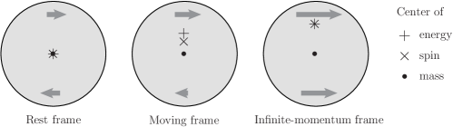
Figure 1: Illustration of the relative positions of the relativistic centers of energy, mass and spin inside a transversely polarized nucleon (the arrows indicate the local momentum seen by the observer). For simplicity, Lorentz contraction effects are not represented. In the rest frame of the nucleon, the three relativistic centers coincide. In a general moving frame they all differ. In the infinite-momentum frame, the relativistic centers of energy and spin merge and are found half a Compton wavelength away from the relativistic center of mass.

There are many interesting observations to make. First, the explicit calculation confirms that the center of the wave packet is nothing but the relativistic center of spin Lorce:2018zpf , which lies on the segment joining the relativistic centers of mass and energy. In the rest frame defined by $\boldsymbol{p}=\boldsymbol{0}$, the three sets of center and spin coincide. If we decompose three-vectors into longitudinal and transverse components relative to $\boldsymbol{p}$

$$\boldsymbol{V}=(\boldsymbol{V}\cdot\hat{\boldsymbol{p}})\,\hat{\boldsymbol{p}}+\boldsymbol{V}_{\!\perp}$$ (65)

with $\hat{\boldsymbol{p}}=\boldsymbol{p}/|\boldsymbol{p}|$, one sees that the longitudinal components of position and spin (i.e. helicity) also coincide in any frame

$$\langle\boldsymbol{R}_{E}\rangle\cdot\hat{\boldsymbol{p}} =\langle\boldsymbol{R}_{M}\rangle\cdot\hat{\boldsymbol{p}}=\langle\boldsymbol{R}_{c}\rangle\cdot\hat{\boldsymbol{p}}=\boldsymbol{\mathcal{R}}\cdot\hat{\boldsymbol{p}},$$ (66)

$$\langle\boldsymbol{S}_{E}\rangle\cdot\hat{\boldsymbol{p}} =\langle\boldsymbol{S}_{M}\rangle\cdot\hat{\boldsymbol{p}}=\langle\boldsymbol{S}_{c}\rangle\cdot\hat{\boldsymbol{p}}=\tfrac{1}{2}\boldsymbol{s}\cdot\hat{\boldsymbol{p}}.$$

Differences appear only in the corresponding transverse components and illustrate why transverse spin is always more complicated than longitudinal spin. In particular, there are three different possible definitions of transverse spin:

• If one defines spin as the internal AM about the relativistic center of energy, then transverse spin is Lorentz contracted

  $$\langle\boldsymbol{S}_{E\perp}\rangle=\gamma^{-1}\,\tfrac{1}{2}\boldsymbol{s}_{\perp}$$ (67)

  with $\gamma=p^{0}/m$ the Lorentz boost factor.

• If one defines instead spin as the internal AM about the relativistic center of mass, then transverse spin is Lorentz dilated

  $$\langle\boldsymbol{S}_{M\perp}\rangle=\gamma\,\tfrac{1}{2}\boldsymbol{s}_{\perp}$$ (68)

  This is expected since in this case internal AM transforms in the same way as total AM, i.e. as the axial-vector part of an antisymmetric rank-two tensor, whose transverse components are known to increase linearly with energy Landau:1951 .

• Finally, if one defines spin as the internal AM about the relativistic center of spin, then transverse spin is invariant under Lorentz boosts

  $$\langle\boldsymbol{S}_{c\perp}\rangle=\tfrac{1}{2}\boldsymbol{s}_{\perp}$$ (69)

  just like longitudinal spin, which is in agreement with the result found in Ref. Bakker:2004ib .

It is seen that the different results for the expectation values of the three kinds of spin operators, in the case of transverse spin, is simply due to the fact that they correspond to different versions of what is meant by the internal AM or “spin”.

Note that in the infinite-momentum frame $|\boldsymbol{p}|\to\infty$, the relativistic center of spin merges with the relativistic center of energy and is found half a Compton wavelength away from the relativistic center of mass when the polarization is purely transverse Burkardt:2002hr ; Burkardt:2005hp ; Lorce:2018zpf

$$\lim_{|\boldsymbol{p}|\to\infty}\left(\boldsymbol{\mathcal{R}}-\langle\boldsymbol{R}_{M}\rangle\right)=\frac{\hat{\boldsymbol{p}}\times\boldsymbol{s}}{2m}=\frac{\hat{\boldsymbol{p}}\times\boldsymbol{s}}{2}\,\frac{\hbar}{mc}.$$ (70)

It may then seem surprising that in this limit $\langle\boldsymbol{S}_{E\perp}\rangle$ vanishes whereas $\langle\boldsymbol{S}_{c\perp}\rangle$ remains non-zero for a state with non-zero transverse polarization. The reason is that the difference in the definition of the internal AM is given by

$$\langle\boldsymbol{S}_{c}\rangle-\langle\boldsymbol{S}_{E}\rangle=\left(\langle\boldsymbol{R}_{E}\rangle-\langle\boldsymbol{R}_{c}\rangle\right)\times\boldsymbol{p}=\frac{(\boldsymbol{p}\times\boldsymbol{s})\times\boldsymbol{p}}{2p^{0}(p^{0}+m)}.$$ (71)

In the infinite-momentum frame, the infinitely small transverse shift is multiplied by an infinitely large momentum, leading to a finite difference.

IV.2 Spin sum rules

We are now ready to derive a generic spin sum rule. By this we mean a decomposition of the expectation value of internal AM into quark and gluon contributions

$$\langle\boldsymbol{S}_{X}\rangle=\sum_{a}\langle\boldsymbol{S}_{X,a}\rangle,\qquad X=E,M,c,$$ (72)

where

$$S^{i}_{X,a}\equiv\int\mathrm{d}^{3}r\,\epsilon^{ijk}\left(r^{j}-\langle R^{j}_{X}\rangle\right)T^{0k}_{a}(r)=J^{i}_{a}-\epsilon^{ijk}\langle R^{j}_{X}\rangle P^{k}_{a}.$$ (73)

Using our master formula (57), we find that the expectation values of the quark and gluon contributions to the total AM are given by

$$\langle\boldsymbol{J}_{a}\rangle=\left(\boldsymbol{\mathcal{R}}\times\boldsymbol{p}+\frac{\boldsymbol{s}}{2}\right)A_{a}(0)+\frac{p^{0}}{2m}\left(\boldsymbol{s}-\frac{\boldsymbol{p}(\boldsymbol{p}\cdot\boldsymbol{s})}{p^{0}(p^{0}+m)}\right)B_{a}(0).$$ (74)

It follows then from Eqs. (54) and (73) that

$$\langle\boldsymbol{S}_{X,a}\rangle=\left[(\boldsymbol{\mathcal{R}}-\langle\boldsymbol{R}_{X}\rangle)\times\boldsymbol{p}+\frac{\boldsymbol{s}}{2}\right]A_{a}(0)+\frac{p^{0}}{2m}\left(\boldsymbol{s}-\frac{\boldsymbol{p}(\boldsymbol{p}\cdot\boldsymbol{s})}{p^{0}(p^{0}+m)}\right)B_{a}(0).$$ (75)

Finally, using the results in Table 1 we obtain the key result of this work

$$\langle\boldsymbol{S}_{X,a}\rangle=\langle\boldsymbol{S}_{X}\rangle A_{a}(0)+\langle\boldsymbol{S}_{M}\rangle B_{a}(0).$$ (76)

Summing over the quark and gluon contributions, we recover the constraints $\sum_{a}A_{a}(0)=1$ and $\sum_{a}B_{a}(0)=0$ arising from Poincaré symmetry. We show in the following that various spin sum rules discussed in the literature simply correspond to particular cases of this remarkable simple-looking formula.

IV.2.1 Helicity sum rule

First, if we restrict ourselves to the longitudinal component, we find the unique situation that we get a sum rule independent of the choice of position vector, i.e. a sum rule with the quark and gluon contributions given by

$$\langle\boldsymbol{S}_{X,a}\rangle\cdot\hat{\boldsymbol{p}}=\frac{\boldsymbol{s}\cdot\hat{\boldsymbol{p}}}{2}\left[A_{a}(0)+B_{a}(0)\right].$$ (77)

For a longitudinally polarized nucleon, we have in particular $\boldsymbol{s}\cdot\hat{\boldsymbol{p}}=1$. This is nothing else than the helicity sum rule derived in Refs. Ji:1996ek ; Ji:1997pf . Since the choices $X=E,M,c$ all give the same result, this explains why the question of the center of the nucleon did not attract much attention in the literature.

IV.2.2 Canonical spin sum rule

If we choose to work with the canonical position $\langle\boldsymbol{R}_{c}\rangle=\boldsymbol{\mathcal{R}}$, we simply have to set $X=c$ in Eq. (76). The quark and gluon contributions to the canonical spin are then given by

$$\langle\boldsymbol{S}_{c,a}\rangle=\frac{\boldsymbol{s}}{2}\,A_{a}(0)+\frac{p^{0}}{2m}\left(\boldsymbol{s}-\frac{\boldsymbol{p}(\boldsymbol{p}\cdot\boldsymbol{s})}{p^{0}(p^{0}+m)}\right)B_{a}(0).$$ (78)

This expression was derived for the first time in Ref. Leader:2011cr by setting the origin at the center of the wave packet (i.e. the relativistic center of spin), and hence computing $\langle\boldsymbol{J}_{a}\rangle_{\boldsymbol{0},\boldsymbol{p},\boldsymbol{s}}=\langle\boldsymbol{S}_{c,a}\rangle_{\boldsymbol{0},\boldsymbol{p},\boldsymbol{s}}$ from Eq. (49). Our phase-space approach generalizes in a straightforward way the derivation to an arbitrary choice of origin, i.e. to arbitrary $\boldsymbol{\mathcal{R}}$, thanks to Eq. (50).

IV.2.3 Covariant spin sum rule

If we are interested in the internal AM about the relativistic center of mass, it suffices to set $X=M$ in Eq. (76). We then find

$$\langle\boldsymbol{S}_{M,a}\rangle=\frac{p^{0}}{2m}\left(\boldsymbol{s}-\frac{\boldsymbol{p}(\boldsymbol{p}\cdot\boldsymbol{s})}{p^{0}(p^{0}+m)}\right)\left[A_{a}(0)+B_{a}(0)\right],$$ (79)

This is the only case where the contributions associated with the $A_{a}$ and $B_{a}$ form factors have the same momentum dependence. In particular, even though $\boldsymbol{S}_{M,a}$ is not conserved, its expectation value is proportional to $\langle\boldsymbol{S}_{M}\rangle$ and hence transforms in a covariant way. This has to do with the fact that $\langle R^{\mu}_{M}\rangle$ transforms as a Lorentz four-vector.

Focusing on the transverse components, we get

$$\langle\boldsymbol{S}_{M\perp,a}\rangle=\gamma\,\frac{\boldsymbol{s}_{\perp}}{2}\left[A_{a}(0)+B_{a}(0)\right]$$ (80)

with $\gamma=p^{0}/m$. This result was derived recently in Ref. Ji:2020hii by computing $\langle J^{i}_{a}\rangle_{\boldsymbol{0},\boldsymbol{p},\boldsymbol{s}}=\epsilon^{ijk}\langle\int\mathrm{d}^{3}r\,r^{j}T^{0k}_{a}(r)\rangle_{\boldsymbol{0},\boldsymbol{p},\boldsymbol{s}}$ from Eq. (49) like in Ref. Leader:2011cr , but this time discarding terms proportional to $p^{j}$ or $p^{k}$ in $\langle\int\mathrm{d}^{3}r\,r^{j}T^{0k}_{a}(r)\rangle_{\boldsymbol{0},\boldsymbol{p},\boldsymbol{s}}$. The authors motivated the latter prescription by the fact that the Pauli-Lubański pseudovector $\langle W^{\mu}\rangle=\frac{1}{2}\,\epsilon^{\mu\alpha\beta\lambda}\langle M_{\alpha\beta}\rangle p_{\lambda}$ does not receive any contribution from terms proportional to $p^{\alpha}$ or $p^{\beta}$ in $\langle M^{\alpha\beta}\rangle$, which were accordingly interpreted as the “contribution coming from the center-of-mass motion” of the nucleon. Unfortunately, we did not find in Ref. Ji:2020hii a clear definition of the center of mass, nor a direct calculation of the contribution from its motion. Moreover, the prescription applies only at the level of expectation values and requires therefore a more rigorous justification from the operator level.

Our phase-space approach combined with the discussion about the relativistic definition of the center of the nucleon from Sec. II justifies and clarifies a posteriori the above ad hoc prescription. Indeed, if we consider the expectation value of spatial moments about the relativistic center of mass, we obtain from the master formula (57)

$$\langle\int\mathrm{d}^{3}r\left(r^{i}-\langle R^{i}_{M}\rangle\right)T^{\mu\nu}_{a}(r)\rangle =\left(\mathcal{R}^{i}-\langle R^{i}_{M}\rangle-\frac{\epsilon^{0i\alpha\beta}\mathcal{S}_{\alpha}p_{\beta}}{2m(p^{0}+m)}\right)\frac{p^{\mu}p^{\nu}A_{a}(0)+m^{2}g^{\mu\nu}\bar{C}_{a}(0)}{p^{0}}$$ (81)

$$\quad+(\delta^{i}_{\lambda}-\delta^{0}_{\lambda}\,\tfrac{p^{i}}{p^{0}})\,\frac{p^{\{\mu}\epsilon^{\nu\}\lambda\alpha\beta}\mathcal{S}_{\alpha}p_{\beta}}{p^{0}m}\,\frac{A_{a}(0)+B_{a}(0)}{2}.$$

According to Table 1, we can write

$$\mathcal{R}^{i}-\langle R^{i}_{M}\rangle=\frac{(\boldsymbol{p}\times\boldsymbol{s})^{i}}{2m(p^{0}+m)}=\frac{\epsilon^{0i\alpha\beta}\mathcal{S}_{\alpha}p_{\beta}}{2m(p^{0}+m)}$$ (82)

showing that the contribution from the motion of the center of the wave packet relative to the center of mass compensates exactly the part associated with the Wigner rotation. The first line in Eq. (81) then vanishes identically and we are left with

$$\langle\int\mathrm{d}^{3}r\left(r^{i}-\langle R^{i}_{M}\rangle\right)T^{\mu\nu}_{a}(r)\rangle=(\delta^{i}_{\lambda}-\delta^{0}_{\lambda}\,\tfrac{p^{i}}{p^{0}})\,\frac{p^{\{\mu}\epsilon^{\nu\}\lambda\alpha\beta}\mathcal{S}_{\alpha}p_{\beta}}{p^{0}m}\,\frac{A_{a}(0)+B_{a}(0)}{2}.$$ (83)

In particular, for the AM we have

$$\epsilon^{ijk}\langle\int\mathrm{d}^{3}r\left(r^{j}-\langle R^{j}_{M}\rangle\right)T^{0k}_{a}(r)\rangle=\epsilon^{ijk}\left[\frac{\epsilon^{kj\alpha\beta}\mathcal{S}_{\alpha}p_{\beta}}{2m}\,\frac{A_{a}(0)+B_{a}(0)}{2}\right],$$ (84)

where the expression inside the square brackets is effectively what one obtains from applying the ad hoc prescription to $\langle\int\mathrm{d}^{3}r\,r^{j}T^{0k}_{a}(r)\rangle_{\boldsymbol{0},\boldsymbol{p},\boldsymbol{s}}$, as was done in Ref. Ji:2020hii . We note however that applying naively the ad hoc prescription to $\langle\boldsymbol{K}_{a}\rangle_{\boldsymbol{0},\boldsymbol{p},\boldsymbol{s}}$ would give a contribution from $\bar{C}_{a}(0)$, while the correct expression derived from Eq. (83) does not.

IV.2.4 A new spin sum rule

For completeness, let us finally consider the internal AM about the relativistic center of energy. Setting $X=E$ in Eq. (76), we get

$$\langle\boldsymbol{S}_{E,a}\rangle=\frac{m}{2p^{0}}\left(\boldsymbol{s}+\frac{\boldsymbol{p}(\boldsymbol{p}\cdot\boldsymbol{s})}{m(p^{0}+m)}\right)A_{a}(0)+\frac{p^{0}}{2m}\left(\boldsymbol{s}-\frac{\boldsymbol{p}(\boldsymbol{p}\cdot\boldsymbol{s})}{p^{0}(p^{0}+m)}\right)B_{a}(0),$$ (85)

To the best of our knowledge, this result is derived for the first time.

Since $\boldsymbol{S}_{E}=\boldsymbol{W}/P^{0}$, one may wonder whether this new spin sum rule is related to the sum rule based on the Pauli-Lubański pseudovector proposed in Ref. Ji:2012vj . Beside the factor of $1/P^{0}$, it appears that the decomposition into quark and gluon contributions is in fact different. In Ref. Ji:2012vj the Pauli-Lubański pseudovector is decomposed as

$$W^{\mu}=\sum_{a}\mathcal{W}^{\mu}_{a}$$ (86)

with the quark and gluon contributions defined as

$$\mathcal{W}^{\mu}_{a}=\frac{1}{2}\,\epsilon^{\mu\alpha\beta\lambda}(M_{a})_{\alpha\beta}P_{\lambda}.$$ (87)

In other words, one has

$$\frac{\boldsymbol{\mathcal{W}}_{\!a}}{P^{0}}=\boldsymbol{J}_{a}+\frac{\boldsymbol{K}_{a}\times\boldsymbol{P}}{P^{0}}$$ (88)

whereas we defined

$$\boldsymbol{S}_{E,a}=\boldsymbol{J}_{a}+\frac{\langle\boldsymbol{K}\rangle\times\boldsymbol{P}_{a}}{P^{0}}$$ (89)

as follows from Eqs. (73) and (64). Clearly, the quark and gluon contributions to $\langle\boldsymbol{S}_{E}\rangle$ are defined relative to the center of energy of the whole system and hence involve $\langle\boldsymbol{K}\rangle$. In contrast, $\langle\boldsymbol{\mathcal{W}}_{\!a}\rangle$ involves only $\langle\boldsymbol{K}_{a}\rangle$ which is related to the energy dipole moment arising from the quark or gluon subsystem Lorce:2018zpf . This explains in particular why $\bar{C}_{a}(0)$ appears in $\langle\boldsymbol{\mathcal{W}}_{\!\perp,a}\rangle$ Leader:2012ar ; Hatta:2012jm ; Harindranath:2013goa ; Leader:2013jra and not in $\langle\boldsymbol{S}_{E\perp,a}\rangle$.

V Conclusions

A spin sum rule is usually understood as a decomposition of the angular momentum about the center of the nucleon into quark and gluon contributions. While the longitudinal spin or helicity sum rule is well established, different transverse spin sum rules have been proposed in the literature. In this paper we show that there is no contradiction between the published results, since they correspond to different definitions of what constitutes the center of the nucleon. Transverse angular momentum is always more complicated in a relativistic theory because, unlike longitudinal angular momentum, it commutes neither with longitudinal boosts nor momentum.

In the literature, spin sum rules are often obtained from the expectation value of the angular momentum operator. The latter has to be treated with care since a naive calculation using momentum eigenstates leads to ambiguous or divergent results. Some papers also make use of the Pauli-Lubański pseudovector but have trouble with providing a physical meaning to the contribution coming from the boost generators, and discard terms asserted to arise from the motion of the center of mass without a clear definition of the latter.

In this work, we stress the importance of defining clearly the center of the nucleon. We review the various possibilities offered in the relativistic context (namely the relativistic centers of energy, mass and spin), and remind in passing that boost generators provide the information about the position of the center of energy. We then define expectation values from a phase-space perspective. This allows us to avoid ambiguities encountered in the standard approach, and to compute for the first time the contribution from the motion of the center of the nucleon.

Our key result is found in Eq. (76) which, together with Table 1, gives the generic expression for the quark and gluon contributions to the nucleon spin, based on the three possible definitions of the center of the nucleon. Projecting on particular spin components with particular choices for the center of the nucleon, we reproduce several spin sum rules reported in the literature. In particular, we show that the new sum rule obtained by Ji and Yuan Ji:2020hii is not in contradiction with the older sum rule derived by Leader Leader:2011cr , but simply relies on a different definition for what is meant by internal angular momentum or spin. Namely, if one requires spin to generate rotations about the center of the nucleon, then one is forced to work with the canonical spin operator, leading to the Leader sum rule. If one requires instead spin to transform in a covariant way, then one is forced to work with the angular momentum about the relativistic center of mass, leading to the Ji and Yuan sum rule. We note that a third sum rule can be obtained based on the angular momentum about the relativistic center of energy or inertia, which has the simplest expression in terms of the Poincaré generators.

References

• (1) B. W. Filippone and X. D. Ji, Adv. Nucl. Phys. 26, 1 (2001).
• (2) S. D. Bass, Rev. Mod. Phys. 77, 1257-1302 (2005).
• (3) C. A. Aidala, S. D. Bass, D. Hasch and G. K. Mallot, Rev. Mod. Phys. 85, 655-691 (2013).
• (4) E. Leader and C. Lorcé, Phys. Rept. 541, no.3, 163-248 (2014).
• (5) M. Wakamatsu, Int. J. Mod. Phys. A 29, 1430012 (2014).
• (6) K. F. Liu and C. Lorcé, Eur. Phys. J. A 52, no.6, 160 (2016).
• (7) A. Deur, S. J. Brodsky and G. F. De Téramond, Rept. Prog. Phys. 82, no.076201 (2019).
• (8) X. Ji, F. Yuan and Y. Zhao, Nature Rev. Phys. 3, no.1, 27-38 (2021).
• (9) R. L. Jaffe and A. Manohar, Nucl. Phys. B 337, 509-546 (1990).
• (10) X. D. Ji, Phys. Rev. Lett. 78, 610-613 (1997).
• (11) B. L. G. Bakker, E. Leader and T. L. Trueman, Phys. Rev. D 70, 114001 (2004).
• (12) E. Leader, Phys. Rev. D 85, 051501 (2012).
• (13) M. Burkardt, Int. J. Mod. Phys. A 18, 173-208 (2003).
• (14) M. Burkardt, Phys. Rev. D 72, 094020 (2005).
• (15) X. Ji, X. Xiong and F. Yuan, Phys. Rev. Lett. 109, 152005 (2012).
• (16) X. Ji, X. Xiong and F. Yuan, Phys. Lett. B 717, 214-218 (2012).
• (17) E. Leader and C. Lorcé, Phys. Rev. Lett. 111, 039101 (2013).
• (18) A. Harindranath, R. Kundu, A. Mukherjee and R. Ratabole, Phys. Rev. Lett. 111, 039102 (2013).
• (19) E. Leader, Phys. Lett. B 720, 120-124 (2013) [erratum: Phys. Lett. B 726, 927-927 (2013)].
• (20) Y. Hatta, K. Tanaka and S. Yoshida, JHEP 02, 003 (2013).
• (21) A. Harindranath, R. Kundu and A. Mukherjee, Phys. Lett. B 728, 63-67 (2014).
• (22) X. Ji, X. Xiong and F. Yuan, Phys. Rev. Lett. 111, 039103 (2013).
• (23) X. Ji and F. Yuan, Phys. Lett. B 810, 135786 (2020).
• (24) C. Lorcé and B. Pasquini, Phys. Lett. B 710, 486-488 (2012).
• (25) C. Lorcé, Eur. Phys. J. C 78, no.9, 785 (2018).
• (26) P. Hoodbhoy, X. D. Ji and W. Lu, Phys. Rev. D 59, 014013 (1999).
• (27) C. Lorcé, L. Mantovani and B. Pasquini, Phys. Lett. B 776, 38-47 (2018).
• (28) C. Lorcé, H. Moutarde and A. P. Trawiński, Eur. Phys. J. C 79, no.1, 89 (2019).
• (29) M. H. L. Pryce, Proc. Roy. Soc. Lond. A 195, 62-81 (1948).
• (30) C. Møller, Commun. Dublin Inst. Advanced Studies A 5, 3 (1949).
• (31) G. N. Fleming, Phys. Rev. 137, B188 (1965).
• (32) T. Choi, J. Korean Phys. Soc. 66, no.6, 877-881 (2015).
• (33) A. D. Fokker, Relativiteitstheorie, P. Noordhoff, Groningen, 1929.
• (34) M. Born and L. Infeld, Proc. Roy. Soc. Lond. A 150, no.869, 141-166 (1935).
• (35) F. J. Belinfante, Physica 7, 449-474 (1940).
• (36) J. K. Lubański, Physica (in French) 9, no.3, 310-324 (1942).
• (37) J. K. Lubański, Physica (in French) 9, no.3, 325-338 (1942).
• (38) C. Møller, Ann. Inst. Henri Poincaré 11, 251-278 (1949).
• (39) M. H. L. Pryce, Proc. Roy. Soc. Lond. A 150, no.869, 166-172 (1935).
• (40) T. Newton and E. P. Wigner, Rev. Mod. Phys. 21, 400-406 (1949).
• (41) N. N. Bogolyubov, A. A. Logunov and I. T. Todorov, Introduction to Axiomatic Quantum Field Theory, Benjamin, Reading, MA, 1975.
• (42) P. K. Schwartz and D. Giulini, Int. J. Geom. Meth. Mod. Phys. 17, no.12, 2050176 (2020).
• (43) B. D. Keister and W. N. Polyzou, Adv. Nucl. Phys. 20, 225-479 (1991).
• (44) J. Krause, J. Math. Phys. 18, 889-893 (1977).
• (45) D. E. Fahnline, AM. J. Phys. 50, 818 (1982).
• (46) E. P. Wigner, Annals Math. 40, 149-204 (1939).
• (47) W. N. Polyzou, W. Glöckle and H. Witala, Few Body Syst. 54, 1667-1704 (2013).
• (48) G. M. Shore and B. E. White, Nucl. Phys. B 581, 409-431 (2000).
• (49) P. Lowdon, K. Y. J. Chiu and S. J. Brodsky, Phys. Lett. B 774, 1-6 (2017).
• (50) S. Cotogno, C. Lorcé and P. Lowdon, Phys. Rev. D 100, no.4, 045003 (2019).
• (51) C. Lorcé and P. Lowdon, Eur. Phys. J. C 80, no.3, 207 (2020).
• (52) R. S. Strichartz, A Guide to Distribution Theory and Fourier Transforms, p. 213, CRC Press, Boca Raton, 1994.
• (53) C. Lorcé, Phys. Rev. Lett. 125, no.23, 232002 (2020).
• (54) E. P. Wigner, Phys. Rev.  40, 749 (1932).
• (55) M. Hillery, R. F. O’Connell, M. O. Scully and E. P. Wigner, Phys. Rept.  106, 121 (1984).
• (56) I. Bialynicki-Birula, P. Gornicki and J. Rafelski, Phys. Rev. D 44, 1825-1835 (1991).
• (57) L. L. Foldy and S. A. Wouthuysen, Phys. Rev. 78, 29-36 (1950).
• (58) M. Pavsic, Adv. Appl. Clifford Algebras 28, no.5, 89 (2018).
• (59) M. Burkardt, Phys. Rev. D 62, 071503 (2000) [erratum: Phys. Rev. D 66, 119903 (2002)].
• (60) I. Y. Kobzarev and L. B. Okun, Zh. Eksp. Teor. Fiz. 43, 1904-1909 (1962).
• (61) H. Pagels, Phys. Rev. 144, 1250-1260 (1966).
• (62) X. D. Ji, Phys. Rev. D 58, 056003 (1998).
• (63) C. Lorcé, Phys. Rev. D 97, no.1, 016005 (2018).
• (64) O. V. Teryaev, Spin structure of nucleon and equivalence principle, arXiv:hep-ph/9904376 [hep-ph].
• (65) S. J. Brodsky, D. S. Hwang, B. Q. Ma and I. Schmidt, Nucl. Phys. B 593, 311-335 (2001).
• (66) L. Landau and E. Lifshitz, Classical Theory of Fields, Addison-Wesley, Reading, 1951.