An algorithm for J-spectral factorization of certain matrix functions

Abstract

The problems of matrix spectral factorization and $J$-spectral factorization appear to be important for practical use in many MIMO control systems. We propose a numerical algorithm for $J$–spectral factorization which extends Janashia–Lagvilava matrix spectral factorization method to the indefinite case. The algorithm can be applied to matrices which have constant signatures for all leading principle submatrices. A numerical example is presented for illustrative purposes.

I Introduction

Spectral factorization plays a prominent role in a wide range of fields in system theory and control engineering. In the scalar case, which arises in systems with single input and single output, the factorization problem is relatively easy and several classical methods exist to perform this task (see a survey paper [1]). The matrix spectral factorization, which arises in multi-dimensional systems, is significantly more difficult. Following Wiener’s original efforts [2], dozens of papers addressed the development of appropriate algorithms. None of the above methods can be implemented directly to solve the $J$-spectral factorization.

The Janashia–Lagvilava method is a relatively new algorithm for matrix spectral factorization [3], [4] which proved to be rather effective [5]. To describe this method of $r\times r$ matrix spectral factorization in a few words, one can say that it first performs a lower-upper triangular factorization with causal entries on the diagonal and then carries out an approximate spectral factorization of principle $m\times m$ submatrices step-by-step, $m=2,3,\ldots,r$. The decisive role in the latter process is played by unitary matrix functions of certain structure, which eliminates many technical difficulties connected with computation.

In the present paper, we extend Janashia-Lagvilava method to $J$-spectral factorization case, by using appropriately chosen $J$-unitary matrix functions instead of aforementioned unitary matrices. So far, the method can be used for matrices which have constant signatures for all leading principle submatrices, however, we hope to remove this restriction in the future work. Furthermore, the method has a potential of identifying a simple necessary and sufficient condition for the existence of $J$-spectral factorization and of being further extended towards the factorization of a wider class of Hermitian matrices.

Performed numerical simulations confirm that the proposed algorithm, whenever applicable, is as effective as the existing matrix spectral factorization algorithm. On several occasions, the algorithm can also deal with the so called singular cases, where the zeros of the determinant occur on the boundary. Like the Janashia–Lagvilava method, the algorithm can be used to $J$-factorize non–rational matrices as well.

II Formulation of the problem

Let

$$S(z)=\begin{pmatrix}s_{11}(z)&s_{12}(z)&\cdots&s_{1r}(z)\\ s_{21}(z)&s_{22}(z)&\cdots&s_{2r}(z)\\ \vdots&\vdots&\vdots&\vdots\\ s_{r1}(z)&s_{r2}(z)&\cdots&s_{rr}(z)\end{pmatrix},$$ (1)

$z\in\mathbb{T}:=\{z\in\mathbb{C}:|z|=1\}$, be a Hermitian $r\times r$ matrix function of constant signature, i.e. $S(z)=S^{*}(z)$ and the number of positive and negative eigenvalues of $S(z)$ are the constants $p$ and $q$, with $p+q=r$, for a.a. $z\in\mathbb{T}$.

$J$-spectral factorization of $S$ is by definition the representation

$$S(z)=S_{+}(z)\,J\,S_{+}^{*}(z),$$ (2)

where $S_{+}$ can be extended to a stable analytic function inside $\mathbb{T}$, the matrix function $S_{+}^{*}$ is the Hermitian conjugate of $S$, and $J=(I_{p}\,,\;-I_{q})$ is the diagonal matrix with $p$ ones and $q$ negative ones on the diagonal. We do not specify the classes to which $S$ and $S_{+}$ belong. For simplicity, one can assume that they are (Laurent) matrix polynomials.

The necessity of factorization (2) arises in $\mathcal{H}_{\infty}$ control [6], [7] and its solution is much more involved than the (standard) spectral factorization of positive definite matrix functions (when $p=r$ and $q=0$). Various algorithms for $J$-spectral factorization appear in the literature[8], [9] mostly for rational matrices.

Below, we present a new algorithm of $J$-spectral factorization which is an extension of Janashia-Lagvilava matrix spectral factorization method. Similarly to this method, we first perform a lower-upper triangular $J$-factorization of (1) with analytic entries on the diagonal. This can be achieved only in the case where all the leading principal minors of $S$ have constant signs almost everywhere on $\mathbb{T}$, therefore, we impose this restriction on (1). Then we recursively $J$-factorize leading principle $m\times m$ submatrices of $S$, $m=2,3,\ldots,r$.

III Notation

For any set $\mathcal{S}$, we denote by $\mathcal{S}^{m\times n}$ the set of $m\times n$ matrices with entries from $\mathcal{S}$.

For a matrix $M\in\mathbb{C}^{r\times r}$ we use the standard notation $M^{T}$ and $M^{*}:=\overline{M}^{T}$ for the transpose and the Hermitian conjugate of $M$. The leading principle $m\times m$ submatrix of $M$, $m\leq r$, is denoted by $[M]_{m\times m}$. The same notation is used for matrix functions as well.

The letter $J$ always denotes a signature, i.e. a square diagonal matrix with entries $\pm 1$ on the diagonal. The sizes and entries of $J$ may vary on different occasions. We say that a Hermitian matrix $A=A^{*}\in\mathbb{C}^{m\times m}$ has the signature $J=(I_{p}\,,\;-I_{q})$ if $A$ has $p$ positive and $q$ negative eigenvalues.

For a fixed signature matrix $J$, the set of $J$-unitary matrices, $\mathcal{U}_{J}$, is a group. Furthermore, $U\in\mathcal{U}_{J}\Longrightarrow U^{T}\in\mathcal{U}_{J}$, since $AJB=J\Longrightarrow BJA=J$.

The set of polynomials is denoted by $\mathcal{P}^{+}$, and the set of Laurent polynomials,

$$P(z)=\sum\nolimits_{k=-n}^{m}p_{k}z^{k},$$ (3)

is denoted by $\mathcal{P}$. The set of Laurent polynomials of degree at most $N$ (i.e. $0\leq n,m\leq N$ in (3)) is denoted by $\mathcal{P}_{N}$, and

$$\mathcal{P}_{N}^{+}=\mathcal{P}_{N}\cap\mathcal{P}^{+}.$$

For Laurent polynomial (3), let

$$\widetilde{P}(z)=\sum\nolimits_{k=-n}^{m}\overline{p_{k}}z^{-k}.$$

Suppose also $\mathcal{P}_{N}^{-}:=\{P:\widetilde{P}\in\mathcal{P}_{N}^{+}\}$. Obviously, $\mathcal{P}_{N}^{-}\cap\mathcal{P}_{N}^{+}$ consists of constant functions only.

A matrix polynomial $\mathbf{U}\in\mathcal{P}^{m\times m}$ is called $J$-unitary if $\mathbf{U}(z)$ is $J$-unitary for every $z\in\mathbb{T}$.

The $k$th Fourier coefficient of an integrable function $f\in L_{1}(\mathbb{T})$ is denoted by $c_{k}\{f\}$. If a function $f$ is square integrable, $f\in L_{2}=L_{2}(\mathbb{T})$, then

$$f(z)=\sum\nolimits_{k=-\infty}^{\infty}c_{k}\{f\}z^{k}\;\;\text{ for a.a. }z\in\mathbb{T},$$

and $\|f\|_{2}=2\pi\sum_{k=-\infty}^{\infty}|c_{k}\{f\}|^{2}$.

An integrable function $f$ is called analytic or causal if its Fourier expansion has the form

$$f\sim\sum\nolimits_{k=0}^{\infty}c_{k}\{f\}z^{k}.$$

It is called stable if $f(z)\not=0$ for each $z$ with $|z|<1$, and it is called optimal if (see, e.g., [10, Th. 17.17]

$$\log|f(0)|=\frac{1}{2\pi}\int_{0}^{2\pi}\log|f(e^{it})|\,dt.$$

For a positive integrable function $f$ defined on $\mathbb{T}$, which satisfies the Paley-Wiener condition

$$\log f\in L_{1},$$

there exists a unique (up to a constant multiple with absolute value 1) causal, stable, and optimal function $f^{+}$ such that

$$f(z)=f^{+}(z)\overline{f^{+}(z)}=|f^{+}(z)|^{2}\;\text{ for a.a. }z\in\mathbb{T}.$$

Such a function $f^{+}$ is called the (canonical) scalar spectral factor of $f$ and it can be given explicitly by the formula

$$f^{+}(z)=\sqrt{f(z)}\exp\left(\frac{1}{2}i\mathcal{C}\big{(}\log f\big{)}(z)\right),$$

where $\mathcal{C}$ stands for the harmonic conjugate of $f$:

$$\mathcal{C}(f)(z)=\frac{1}{2\pi}(P)\int_{0}^{2\pi}f(e^{it})\cot\frac{t-\tau}{2}\,d\tau,\;\;\;z=e^{it}.$$

This formula is the core of existing Exp-Log algorithm for scalar spectral factorization. It is the claim of well-known Fejér-Riesz lemma that if, in addition, $f\in\mathcal{P}_{N}$, then $f^{+}\in\mathcal{P}_{N}^{+}$. In Section V, we use the special notation

$$f^{+}=\sqrt[+]{f}$$ (4)

for the scalar spectral factor.

Finally, $\delta_{ij}$ stands for the Kronecker delta, i.e. $\delta_{ij}=1$ if $i=j$ and $\delta_{ij}=0$ otherwise.

IV The main observation

In this section we generalize the main theorem of Janashia-Lagvilava method for $J$-unitary matrices.

Theorem 1

(cf. [4, Th. 1]) Let $F$ be an $m\times m$ matrix function of the form

$$F=\begin{pmatrix}1&0&\cdots&0&0\\ 0&1&\cdots&0&0\\ \vdots&\vdots&\vdots&\vdots&\vdots\\ 0&0&\cdots&1&0\\ \zeta^{-}_{1}&\zeta^{-}_{2}&\cdots&\zeta^{-}_{m-1}&f^{+}\end{pmatrix},$$ (5)

where

$$\zeta^{-}_{j}\in\mathcal{P}_{N}^{-},\;j=1,2,\ldots,m-1;\;f^{+}\in\mathcal{P}_{N}^{+},\;f^{+}(0)\not=0,$$ (6)

for some positive integer $N$, and let $J$ be an arbitrary signature. Then (almost surely) there exists a $J$-unitary matrix function $U$ of the form

$$U=\begin{pmatrix}u_{11}&u_{12}&\cdots&u_{1m}\\ u_{21}&u_{22}&\cdots&u_{2m}\\ \vdots&\vdots&\vdots&\vdots\\ u_{m-1,1}&u_{m-1,2}&\cdots&u_{m-1,m}\\[8.53581pt] \widetilde{u_{m1}}&\widetilde{u_{m2}}&\cdots&\widetilde{u_{mm}}\\ \end{pmatrix},$$ (7)

where

$$u_{ij}\in\mathcal{P}_{N}^{+},\;\;i,j=1,2,\ldots,m,$$ (8)

with constant determinant, such that

$$FU\in(\mathcal{P}^{+}_{N})^{m\times m}.$$ (9)

Remark 1

A sketch of the proof below indicates the isolated cases where the theorem fails to hold. This is the sense in which we use the term “almost surely”. Whenever the solution exists, it is constructed explicitly.

The proof follows literally the proof of Theorem 1 in [4]. We need only to change signs of some expressions accordingly. By this way, we naturally arrive at $J$-unitary matrix functions instead of unitary ones. Indeed, for given functions $\zeta^{-}_{j}$, $j=1,2,\ldots,m-1$, $f^{+}$ satisfying (6), and the signature $J={\rm diag}(J_{1},J_{2},\ldots,J_{m-1},1)$, we consider the following system of $m$ conditions (cf. (15) in [4])

$$\begin{cases}\zeta^{-}_{1}x_{m}-J_{1}\cdot f^{+}\widetilde{x_{1}}\in\mathcal{P}^{+},\\ \zeta^{-}_{2}x_{m}-J_{2}\cdot f^{+}\widetilde{x_{2}}\in\mathcal{P}^{+},\\ \cdot\hskip 28.45274pt\cdot\hskip 28.45274pt\cdot\\ \zeta^{-}_{m-1}x_{m}-J_{m-1}\cdot f^{+}\widetilde{x_{m-1}}\in\mathcal{P}^{+},\\ \zeta^{-}_{1}x_{1}+\zeta^{-}_{2}x_{2}+\ldots+\zeta^{-}_{m-1}x_{m-1}+f^{+}\widetilde{x_{m}}\in\mathcal{P}^{+},\end{cases}$$ (10)

where $\big{(}x_{1},x_{2},\ldots,x_{m}\big{)}^{T}\in(\mathcal{P}^{+}_{N})^{m\times 1}$ is the unknown vector function. We say that a vector function

$$\mathbf{u}=\big{(}u_{1},u_{2},\ldots,u_{m}\big{)}^{T}\in(\mathcal{P}^{+}_{N})^{m\times 1}$$ (11)

is a solution of (10) if and only if all the conditions in (10) are satisfied whenever $x_{i}=u_{k}$, $i=1,2,\ldots,m$.

We make essential use of the following

Lemma 1

Let (6) hold and let

$$\mathbf{u}=\big{(}u_{1},u_{2},\ldots,u_{m}\big{)}^{T}\in(\mathcal{P}_{N}^{+})^{m\times 1}$$

$$\mathbf{v}=\big{(}v_{1},v_{2},\ldots,v_{m}\big{)}^{T}\in(\mathcal{P}_{N}^{+})^{m\times 1}$$

be two $($possibly identical$)$ solutions of the system (10). Then

$$\sum_{k=1}^{m-1}J_{k}u_{k}\widetilde{v_{k}}+\widetilde{u_{m}}v_{m}=\operatorname{const}.$$ (12)

Proof: Substituting the functions $v$ in the first $m-1$ conditions and the functions $u$ in the last condition of (10), and then multiplying the first $m-1$ conditions by $u$ and the last condition by $v_{m}$, we get

$$\begin{cases}\zeta^{-}_{1}v_{m}u_{1}-J_{1}\cdot f^{+}\widetilde{v_{1}}u_{1}\in\mathcal{P}^{+},\\ \zeta^{-}_{2}v_{m}u_{2}-J_{2}\cdot f^{+}\widetilde{v_{2}}u_{2}\in\mathcal{P}^{+},\\ \cdot\hskip 28.45274pt\cdot\hskip 28.45274pt\cdot\\ \zeta^{-}_{m-1}v_{m}u_{m-1}-J_{m-1}\cdot f^{+}\widetilde{v_{m-1}}u_{m-1}\in\mathcal{P}^{+},\\ \zeta^{-}_{1}u_{1}v_{m}+\zeta^{-}_{2}u_{2}v_{m}+\ldots+\zeta^{-}_{m-1}u_{m-1}v_{m}+f^{+}\widetilde{u_{m}}v_{m}\in\mathcal{P}^{+}.\end{cases}$$

Subtracting the first $m-1$ conditions from the last condition in the latter system, we get

$$f^{+}\left(\sum_{k=1}^{m-1}J_{k}u_{k}\widetilde{v_{k}}+\widetilde{u_{m}}v_{m}\right)\in\mathcal{P}^{+}.$$ (13)

Since the second multiple in (13) belongs to $\mathcal{P}_{N}$, taking into account the last condition in (6), we get

$$\sum_{k=1}^{m-1}J_{k}u_{k}\widetilde{v_{k}}+\widetilde{u_{m}}v_{m}\in\mathcal{P}_{N}^{+}.$$

We can interchange the roles of $u$ and $v$ in the above discussion to get in a similar manner that

$$\sum_{k=1}^{m-1}J_{k}v_{k}\widetilde{u_{k}}+\widetilde{v_{m}}u_{m}\in\mathcal{P}_{N}^{+}.$$

Consequently, the function in (12) belongs to $\mathcal{P}_{N}^{+}\cap\mathcal{P}_{N}^{-}$, which implies (12). $\blacksquare$

The proof of Theorem 1 proceeds as follows. We search for a nontrivial polynomial solution

$$\mathbf{x}=\big{(}x_{1},x_{2},\ldots,x_{m}\big{)}^{T}\in(\mathcal{P}_{N}^{+})^{m\times 1}$$ (14)

of the system (10), where

$$x_{i}(z)=\sum_{n=0}^{N}a_{in}z^{n},\;\;\;i=1,2,\ldots,m,$$ (15)

and explicitly determine the coefficients $a_{in}$. We will find such $m$ linearly independent solutions of (10) which appear to be $m$ different columns of (7)

Equating all the Fourier coefficients with non-positive indices of the functions in the left-hand side of (10) to zero, except the $0$th coefficient of the $j$th function which we set equal to $1$, we get the following system of algebraic equations in the block matrix form which we denote by $\mathbb{S}_{j}$:

$$\mathbb{S}_{j}:=\begin{cases}\Gamma_{1}X_{m}-J_{1}D\overline{X_{1}}={\bf 0},\\ \Gamma_{2}X_{m}-J_{2}D\overline{X_{2}}={\bf 0},\\ \;\;\;\;\;\;\;\;\;\;\\ \Gamma_{j}X_{m}-J_{j}D\overline{X_{j}}={\bf 1},\\ \;\;\;\;\;\;\;\;\;\;\\ \Gamma_{m-1}X_{m}-J_{m-1}D\overline{X_{m-1}}={\bf 0},\\ \Gamma_{1}X_{1}+\Gamma_{2}X_{2}+\ldots+\Gamma_{m-1}X_{m-1}+D\overline{X_{m}}={\bf 0}\;.\end{cases}$$ (16)

Here the following matrix notation is used:

$$D=\begin{pmatrix}d_{0}&d_{1}&d_{2}&\cdots&d_{N-1}&d_{N}\\ 0&d_{0}&d_{1}&\cdots&d_{N-2}&d_{N-1}\\ 0&0&d_{0}&\cdots&d_{N-3}&d_{N-2}\\ \cdot&\cdot&\cdot&\cdots&\cdot&\cdot\\ 0&0&0&\cdots&0&d_{0}\end{pmatrix},\;\;$$

$$\Gamma_{i}=\begin{pmatrix}\gamma_{i0}&\gamma_{i1}&\gamma_{i2}&\cdots&\gamma_{i,N-1}&\gamma_{iN}\\ \gamma_{i1}&\gamma_{i2}&\gamma_{i3}&\cdots&\gamma_{iN}&0\\ \gamma_{i2}&\gamma_{i3}&\gamma_{i4}&\cdots&0&0\\ \cdot&\cdot&\cdot&\cdots&\cdot&\cdot\\ \gamma_{iN}&0&0&\cdots&0&0\end{pmatrix},$$

$i=1,2,\ldots,m-1$, where

$$f^{+}(z)=\sum_{n=0}^{N}d_{n}z^{n}\;\text{ and }\;\zeta^{-}_{i}(z)=\sum_{n=0}^{N}\gamma_{in}z^{-n};$$

$${\bf 0}=(0,0,\ldots,0)^{T}\text{ and }{\bf 1}=(1,0,0,\ldots,0)^{T}\in\mathbb{C}^{N+1}.$$

The column vectors

$$X_{i}=(a_{i0},a_{i1},\ldots,a_{iN})^{T},\;\;i=1,2,\ldots,m,$$

(see (15)) are the unknowns.

Since $d_{0}=f^{+}(0)\not=0$ (see (6)), the matrix $D$ is invertible. Hence, determining $X_{i}$, $i=1,2,\ldots,m-1$, from the first $m-1$ equations of (16),

$$X_{i}=J_{i}\left(\overline{D^{-1}}\;\overline{\Gamma_{i}}\;\overline{X_{m}}-\delta_{ij}\overline{D^{-1}}\;{\bf 1}\right),$$ (17)

$i=1,2,\ldots,m-1$, and then substituting them in the last equation of (16), we get

$$J_{1}\Gamma_{1}\,\overline{D^{-1}}\;\overline{\Gamma_{1}}\;\overline{X_{m}}+J_{2}\Gamma_{2}\,\overline{D^{-1}}\;\overline{\Gamma_{2}}\;\overline{X_{m}}+\cdots$$

$$+J_{m-1}\Gamma_{m-1}\,\overline{D^{-1}}\;\overline{\Gamma_{m-1}}\;\overline{X_{m}}+D\;\overline{X_{m}}=J_{j}\Gamma_{j}\,\overline{D^{-1}}\,{\bf 1}$$

(it is assumed that the right-hand side is equal to ${\bf 1}$ when $j=m$) or, equivalently,

$$(J_{1}\Theta_{1}\,{\Theta_{1}^{*}}+J_{2}\Theta_{2}\,{\Theta_{2}^{*}}+\!\ldots\!+J_{m-1}\Theta_{m-1}\,{\Theta_{m-1}^{*}}+I_{N+1})\,\overline{X_{m}}$$

$$=J_{j}D^{-1}\,\Gamma_{j}\,\overline{D^{-1}}\,{\bf 1},$$ (18)

where

$$\Theta_{i}=D^{-1}\,\Gamma_{i}\,,\;\;i=1,2,\ldots,m-1$$

(we wrote $\Theta^{*}$ instead of $\overline{\Theta}$ because $\Theta^{T}=\Theta$).

For each $j=1,2,\ldots,m$, (18) is a linear algebraic system of $N+1$ equations with $(N+1)$ unknowns. This system (18) and consequently (16) has the unique solution for each $j=1,2,\ldots,m$ if and only if

$$\det(\Delta)\not=0,\;\text{ where }\;\Delta=\sum\nolimits_{k=1}^{m-1}J_{k}\Theta\Theta^{*}+I_{N+1}\,.$$ (19)

Remark 2

Unlike the spectral factorization, where $\Delta$ is always positive definite and (19) holds, there are isolated indefinite cases where (19) does not hold. However, we can assume that (19) holds (see Remark 1) and proceed with solution of (10).

Remark 3

As in the spectral factorization case (see [4, Appendix]) the matrix $\Delta$ has a displacement structure of rank $m$ with respect to $Z$, where $Z$ is the upper triangular $(N+1)\times(N+1)$ matrix with 1’s on the first superdiagonal and 0’s elsewhere (i.e., a Jordan block with eigenvalue 0). Namely,

$$R_{Z}\Delta:=\Delta-Z\Delta Z^{*}=AJA^{*},$$

where $A$ is the $(N+1)\times m$ matrix which has $i$-th column equal to the first column of $\Theta_{i}$, $i=1,2,\ldots,m-1$, and the last column is equal to $(0,0,\ldots,0,1)\in\mathbb{C}^{N+1}$. Consequently, the triangular factorization of $\Delta$ can be performed in $O(mN^{2})$ operations instead of the traditional $O(N^{3})$ ones, as it is described in [11, Appendix F.1]. This substantially reduces the amount of operations if $N\gg m$.

Finding the matrix vector $\overline{X_{m}}$ from (18) and then determining $X_{1},X_{2},\ldots,X_{m-1}$ from (17), we get the unique solution of $\mathbb{S}_{j}$. To indicate its dependence on $j$, we denote the solution of $\mathbb{S}_{j}$ by $(X_{1}^{j},X_{2}^{j},\ldots,X_{m-1}^{j},X_{m}^{j})$,

$$X_{i}^{j}:=(a_{i0}^{j},a_{i1}^{j},\ldots,a_{iN}^{j})^{T},\;\;\;i=1,2,\ldots,m,$$ (20)

so that if we construct a matrix function $V$,

$$V=\begin{pmatrix}v_{11}&v_{12}&\cdots&v_{1m}\\ v_{21}&v_{22}&\cdots&v_{2m}\\ \vdots&\vdots&\vdots&\vdots\\ v_{m-1,1}&v_{m-1,2}&\cdots&v_{m-1,m}\\[8.53581pt] \widetilde{v_{m1}}&\widetilde{v_{m2}}&\cdots&\widetilde{v_{mm}}\\ \end{pmatrix},$$ (21)

by letting (see (20))

$$v_{ij}(z)=\sum_{n=0}^{N}a_{in}^{j}z^{n},\;\;\;1\leq i,j\leq m,$$ (22)

then columns of (21) are solutions of the system (20). Hence, because of the last equation in (15),

$$FV\in(\mathcal{P}^{+}_{N})^{m\times m}$$

and, by virtue of Lemma 1,

$$V(z)\,J\,V^{*}(z)=C,$$ (23)

where $C$ is a constant Hermitian matrix with signature $J$. It can be also proved that (see [4, p. 2322, II]) that

$$\det V(z)={\rm const}.$$

Decomposing the matrix $C$ as

$$C=C_{0}J\,C_{0}^{*},\;\text{ where }C_{0}=V(1),$$ (24)

equations (23) and (24) imply

$$C_{0}^{-1}V(z)\,J\,(C_{0}^{-1}V(z))^{*}=J.$$

Hence,

$$U=C_{0}^{-1}V$$

is the required $J$-unitary matrix and it can be numerically computed by using the above equations. $\blacksquare$

V Description of the algorithm

In this section we provide computational procedures for $J$-factorization of (1) which are similar to corresponding procedures presented in [4].

Procedure 1. First we perform the lower-upper triangular $J$-factorization of $S$:

$$S(z)=M(z)\,J\,M^{*}(z).$$ (25)

Here

$$M=\begin{pmatrix}f^{+}_{1}&0&\cdots&0&0\\ \xi_{21}&f^{+}_{2}&\cdots&0&0\\ \vdots&\vdots&\vdots&\vdots&\vdots\\ \xi_{r-1,1}&\xi_{r-1,2}&\cdots&f^{+}_{r-1}&0\\ \xi_{r1}&\xi_{r2}&\cdots&\xi_{r,r-1}&f^{+}_{r}\end{pmatrix},$$

where $f^{+}_{m}$, $m=1,2,\ldots,r$, are stable analytic functions (we also assume that all entries are square integrable). Such factorization can always be achieved under the restriction that $\det[S]_{m\times m}$ has constant sign almost everywhere on $\mathbb{T}$ for each $m=1,2,\ldots,r$. This happens, for example, if all principle minors are non-singular everywhere on $\mathbb{T}$, however, this condition is not necessary. We can apply the similar recursive formulas as for usual Cholesky factorization: $f_{1}^{+}=\sqrt[+]{J_{1}s_{11}}$, $\xi_{i1}=J_{1}s_{i1}/\overline{f_{1}^{+}}$, $i=2,3,\ldots,r$;

$${f_{j}^{+}}=\sqrt[+]{J_{j}\left(s_{jj}-\sum\nolimits_{k=1}^{j-1}J_{k}\xi_{jk}\overline{\xi_{jk}}\right)},\;j=2,3,\ldots,r;$$

$$\xi_{ij}=J_{j}\left(s_{ij}-\sum\nolimits_{k=1}^{j-1}J_{k}\xi_{ik}\overline{\xi_{jk}}\right)/\overline{f_{j}^{+}},$$

$j=2,3,\ldots,r-1$, $i=j+1,j+2,\ldots,r$, assuming that $\sqrt[+]{\cdot}$ performs the scalar spectral factorization (see (4)). In actual computations, one can perform factorization (25) pointwise in frequency domain for selected values of $z\in\mathbb{T}$.

Procedure 2. We approximate $M$ in $L_{2}$ keeping only a finite number of coefficients with negative indices in the Fourier expansions of the entries of $M$. For the convenience of computations, we take a different number of these coefficients for different entries below the main diagonal. Namely, for a large positive integer $N$, let

$$M_{N}=\begin{pmatrix}f^{+}_{1}&0&\cdots&0&0\\[2.84526pt] \xi^{[N]}_{21}&f^{+}_{2}&\cdots&0&0\\[2.84526pt] \vdots&\vdots&\vdots&\vdots&\vdots\\[2.84526pt] \xi^{[(r-2)N]}_{r-1,1}&\xi^{[(r-3)N]}_{r-1,2}&\cdots&f^{+}_{r-1}&0\\[2.84526pt] \xi^{[(r-1)N]}_{r1}&\xi^{[(r-2)N]}_{r2}&\cdots&\xi^{[N]}_{r,r-1}&f^{+}_{r}\end{pmatrix}$$ (26)

where $\xi^{[{N}]}_{ij}(z)=\sum_{n=-{N}}^{\infty}c_{n}\{\xi_{ij}\}z^{n}$, $2\leq i\leq r$, $1\leq j<r$. Let

$$S_{N}(z)=M_{N}(z)\,J\,M_{N}^{*}(z).$$

Procedure 3. We compute explicitly $S_{N}^{+}$, a $J$-spectral factor of $S_{N}$. This is done recursively with respect to $m$. Namely, we represent $S_{N}^{+}$ as

$$S_{N}^{+}=M_{N}\mathbf{U}_{1}\mathbf{U}_{2}\mathbf{U}_{3}\ldots\mathbf{U}_{r},$$

where each $U_{m}$ is $J$-unitary and has the block matrix form

$$\mathbf{U}_{m}(t)=\begin{pmatrix}U_{m}(t)&0\\ 0&I_{r-m}\end{pmatrix},$$ (27)

$m=2,3,\ldots r$. Furthermore, each $[Q_{m}]_{m\times m}$ is $J$-spectral factor of $[S_{N}]_{m\times m}$

$$[S_{N}]_{m\times m}=[Q_{m}]_{m\times m}\,[J]_{m\times m}\,[Q_{m}]_{m\times m}^{*},$$ (28)

where

$$Q_{m}=M_{N}\mathbf{U}_{1}\mathbf{U}_{2}\mathbf{U}_{3}\ldots\mathbf{U}_{m}.$$

We take $\mathbf{U}_{1}=I_{r}$ and then (28) is valid for $m=1$. Assume that $\mathbf{U}_{2}(t)$,$\mathbf{U}_{2}(t)$$\ldots$,$\mathbf{U}_{m-1}(t)$ have already been constructed so that (28) holds when $m$ is replaced by $m-1$ and suppose the last row of $[Q_{m-1}]_{m\times m}$ is $[\zeta^{m-1}_{1},\zeta^{m-1}_{2},\ldots,\zeta^{m-1}_{m-1},f_{m}^{+}]$. Then we construct the next $J$-unitary matrix (27) by performing the following operations:

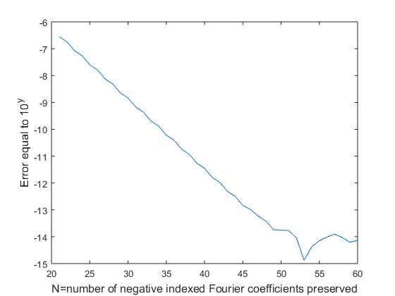
Figure 1: Error in $J$-spectral factorization of matrix (29)

Step 1. Construct a matrix function $F(t)$ of the form (5), where

$$\zeta^{-}_{j}(z)=\sum_{n=-(m-1)N}^{0}c_{n}\big{\{}\zeta^{m-1}_{j}\big{\}}\,z^{n},\;\;\;j=1,2,\ldots,m-1,$$

and

$$f^{+}(z)=\sum\nolimits^{(m-1)N}_{n=0}c_{n}\{f_{m}^{+}\}\,z^{n}\,.$$

Step 2. Using Theorem 1, construct $U$ of the form (7), where $u_{ij}\in\mathcal{P}^{+}_{(m-1)N}$, $1\leq i,j\leq m$, so that (9) would hold.

Step 3. Define $\mathbf{U}_{m}$ by the equation (27) where $U_{m}=U$ is found in Step 2.

VI Numerical Example

To illustrate our approach, we present an approximate $J$-factorization of the following polynomial matrix function $S=$

$$\begin{pmatrix}-8z^{-1}-19-8z&-39z^{-1}-73-28z\\ -28z^{-1}-73-39z&-137z^{-1}-286-137z\end{pmatrix}.$$ (29)

This matrix satisfies the conditions imposed on $S$ in order for the algorithm to be applicable, namely $s_{11}(z)$ and

$$\det S(z)=4(z^{-2}-2+z^{2})=4(z^{-2}-1)(1-z^{2})$$

are both negative for $z\in\mathbb{T}$. However, the matrix $S(z)$ is singular for $z=-1$ and $1$, which usually complicates the factorization process. The $J$-factorization of (29) is known in advance due to the corresponding example of the singular matrix in [5]:

$$S(z)=S_{+}(z)\begin{pmatrix}-1&0\\ 0&1\end{pmatrix}S_{+}^{*}(z),$$

where

$$S_{+}(z)=\begin{pmatrix}4+2z&1\\ 14+10z&3+z\end{pmatrix}.$$ (30)

However, we follow the steps of the proposed algorithm to produce an approximate result.

The triangular $J$-factorization of $S$ has the form

$$S(z)=M(z)\begin{pmatrix}-1&0\\ 0&1\end{pmatrix}M^{*}(z)$$

where $M(z)=$

$$\begin{pmatrix}3.824\ldots+z\cdot 2.092\ldots&0\\[5.69054pt] \dfrac{28z^{-1}+73+39z}{z^{-1}\cdot 2.092\ldots+3.824\ldots}&\dfrac{1-z^{2}}{3.824\ldots+z\cdot 2.092\ldots}\end{pmatrix}$$

with

$$f_{1}^{+}(z):=3.824\ldots+z\cdot 2.092\ldots=\sqrt[+]{8z^{-1}+19+8z}$$

and

$$f_{2}^{+}(z):=(1-z^{2})=\sqrt[+]{-z^{-2}+2-z^{2}}.$$

We expand $\xi_{21}=-s_{21}/\widetilde{f^{+}_{1}}$ into Fourier series by the division of polynomials and, for a positive integer $N$, approximate it by “cutting the tail”:

$$\xi_{21}(z)\approx\xi_{21}^{[N]}(z)=\sum\nolimits_{k=-N}^{\infty}c_{k}\{\xi_{21}\}z^{k}.$$

Thus we get the approximation of $S$ by

$$S_{N}=\begin{pmatrix}f_{1}^{+}&0\\ \xi_{21}^{[N]}&f_{2}^{+}\end{pmatrix}\begin{pmatrix}-1&0\\ 0&1\end{pmatrix}\begin{pmatrix}f_{1}^{+}&0\\ \xi_{21}^{[N]}&f_{2}^{+}\end{pmatrix}^{*}$$

and we obtain its $J$-spectral factor $S_{N}^{+}$ by finding explicitly a $J$-unitary matrix $U=U_{N}$ as it is described in Section V:

$$S_{N}^{+}=\begin{pmatrix}f_{1}^{+}&0\\ \xi_{21}^{[N]}&f_{2}^{+}\end{pmatrix}\cdot U.$$

The computation results coincide with the exact answer (30) within 16 digits (the Matlab double precision) for $N=53$.

A total computational time to achieve this accuracy is less than 0.02 sec (on a laptop with the characteristics: Intel(R) Core(TM) i7 8650U CPU, 1.90 GHz, RAM 16.00 Gb). Fig. 1 shows how this accuracy increases with increasing $N$.

References

• [1] A. H. Sayed and T. Kailath, “A survey of spectral factorization methods,” Numer. Linear Algebra Appl., vol. 8, pp. 467–496, 2001, numerical linear algebra techniques for control and signal processing.
• [2] N. Wiener and P. Masani, “The prediction theory of multivariate stochastic processes. II. The linear predictor,” Acta Math., vol. 99, pp. 93–137, 1958.
• [3] G. Janashia and E. Lagvilava, “A method of approximate factorization of positive definite matrix functions,” Studia Math., vol. 137, pp. 93–100, 1999.
• [4] G. Janashia, E. Lagvilava, and L. Ephremidze, “A new method of matrix spectral factorization,” IEEE Trans. Inform. Theory, vol. 57, pp. 2318–2326, 2011.
• [5] L. Ephremidze, F. Saied, and I. M. Spitkovsky, “On the algorithmization of Janashia-Lagvilava matrix spectral factorization method,” IEEE Trans. Inform. Theory, vol. 64, pp. 728–737, 2018.
• [6] B. A. Francis, A course in $H_{\infty}$ control theory.   Springer-Verlag, Berlin, 1987.
• [7] H. Kimura, Chain-scattering approach to $H^{\infty}$ control.   Birkhäuser Boston, Inc., Boston, MA, 1997.
• [8] H. Kwakernaak and M. Šebek, “Polynomial $J$-spectral factorization,” IEEE Trans. Automat. Control, vol. 39, pp. 315–328, 1994.
• [9] J. Stefanovski, “Discrete $J$-spectral factorization of possibly singular polynomial matrices,” Systems Control Lett., vol. 53, pp. 127–140, 2004.
• [10] W. Rudin, Real and complex analysis, 3rd ed.   McGraw-Hill Book Co., New York, 1987.
• [11] T. Kailath, B. Hassibi, and A. H. Sayed, Linear Estimation.   Prentice-Hall, Inc., Englewood Cliffs, N.J., 1999.