One-loop form factors for $H\rightarrow\gamma^{*}\gamma^{*}$
in $R_{\xi}$ gauge

Abstract

In this paper, we present general one-loop form factors for $H\rightarrow\gamma^{*}\gamma^{*}$ in $R_{\xi}$ gauge, considering all cases of two on-shell, one on-shell and two off-shell for final photons. The calculations are performed in standard model and in arbitrary beyond the standard models which charged scalar particles may be exchanged in one-loop diagrams. Analytic results for the form factors are shown in general forms which are expressed in terms of the Passarino-Veltman functions. We also confirm the results in previous computations which are available for the case of two on-shell photons. The $\xi$-independent of the result is also discussed. We find that numerical results are good stability with varying $\xi=0,1$ and $\xi\rightarrow\infty$.

1 Introduction

One of the main targets at future colliders such as high luminosity the Large Hadron Collider (HL-LHC) [1, 2] and future lepton colliders [3] is to measure the properties of the Standard Model Higgs boson ($H$) precisely. All the Higgs decay modes, Higgs boson productions and the couplings of Higgs to fermions, gauge bosons are measured precisely. From these activities, one may explore the nature of the Higgs sector as well as search for new physics.

Among Higgs decay modes,the decay of Higgs boson into two photons is the most important for several following reasons. First, this arises at first at one-loop diagrams. Therefore, it is sensitive with new physics which the charged scalar particles may exchange in the loop diagrams. As a result, the calculations for one-loop and higher-loop contributions to the decay amplitudes of $H\rightarrow\gamma\gamma$ play a key role in controlling the standard model background, constraining new physics parameters. Secondly, one-loop form factors for $H\rightarrow\gamma\gamma^{*},\gamma^{*}\gamma^{*}$ ($\gamma^{*}$ presents for a virtual photon) are useful for studying Higgs productions and its properties at $\gamma\gamma,e\gamma$ colliders [4, 5, 6, 7, 8, 9, 10]. Last but not least, the decay processes $H\rightarrow\gamma^{*}\gamma\rightarrow f\bar{f}\gamma,\gamma^{*}\gamma^{*}\rightarrow 4$ fermions provide a crucial tool for controlling background for $H\rightarrow f\bar{f}\gamma,H\rightarrow 4$ fermions at future colliders.

Many calculations for one-loop contributions to $H\rightarrow\gamma\gamma$ within standard model (SM) and its extensions have been presented in [11, 12, 13, 14, 15, 16, 17, 18, 19, 20, 21, 22, 23, 24, 25], also in the references therein. More recently, the authors of Ref. [26] argue that one-loop W boson contributions to $H\rightarrow\gamma\gamma$ lead to different expressions in unitary and in general $R_{\xi}$ gauges. Latter, the results in Ref. [27] confirm again the gauge invariance of $H\rightarrow\gamma\gamma$. On the other hand, the Higgs production in two-photon process and one-loop transition form factor for $H\rightarrow\gamma\gamma^{*}$ has been computed in Ref. [5]. Furthermore, the Higgs production at $e^{-}\gamma$ collision via the process $e^{-}\gamma\rightarrow e^{-}H\rightarrow e^{-}b\bar{b}$ has been considered in Ref. [6]. To the best of our knowledge, there are not available one-loop form factors for decay channel $H\rightarrow\gamma^{*}\gamma^{*}$.

In this paper, the detailed calculations for one-loop form factors for $H\rightarrow\gamma^{*}\gamma^{*}$ in $R_{\xi}$ gauge are presented, considering all cases of two on-shell, one on-shell and two off-shell for final photons. The computations are performed within standard model and in arbitrary beyond the standard model (BSM) which the charged scalar particles may exchange in one-loop Feynman diagrams. The analytical results for the form factors are expressed in terms of Passarino-Veltman functions which are presented in standard forms of LoopTools [30]. Analytic formulas for these functions are well-known and their numerical evaluations can be generated by using LoopTools. In our present paper, analytic results are shown in $R_{\xi=1}$ for $H\rightarrow\gamma^{*}\gamma^{*}$ and $\gamma\gamma^{*}$. While one-loop form factor formulas for $H\rightarrow\gamma\gamma$ are presented in both ’t Hooft-Veltman and general $R_{\xi}$ gauges. We also verify the previous calculations in the case of two on-shell photons. The $\xi$-independent of the result is also discussed. We show the numerical checks for one-loop form factors $H\rightarrow\gamma\gamma$ with varying $\xi=0,1$ and $\xi\rightarrow\infty$.

The layout of the paper is as follows: In section 2, we present briefly one-loop tensor reduction method. We then present the evaluations in detail for one-loop form factors of Higgs decay into two photons. Analytical results for the form factors with two real photons, one virtual photon, two virtual photons are shown in this section. Conclusions and outlook are devoted in section 3. In appendices, Feynman rules and one-loop amplitude for the decay channel are discussed.

2 Calculations

In this calculation, we apply the technique for the reduction of one-loop tensor integrals developed in Ref. [28]. In following section, we describe briefly this approach. In general, one-loop one-, two- and three-point tensor integrals with rank $P$ are defined as:

$$\{A;B;C\}^{\mu_{1}\mu_{2}\cdots\mu_{P}}=\int\frac{d^{d}k}{(2\pi)^{d}}\dfrac{k^{\mu_{1}}k^{\mu_{2}}\cdots k^{\mu_{P}}}{\{D_{1};D_{1}D_{2};D_{1}D_{2}D_{3}\}}.$$ (1)

In this formula, $D_{j}$ for $j=1,2,3$ are the inverse Feynman propagators which are given:

$$D_{j}=(k+q_{j})^{2}-m_{j}^{2}+i\rho.$$ (2)

Where $q_{j}$ are defined as $q_{j}=\sum\limits_{i=1}^{j}p_{i}$, $p_{i}$ are external momenta; $m_{j}$ are internal masses. The reduction formulas for one-loop one-, two-, three-points tensor integrals up to rank $P=3$ are written explicitly as follows [28]:

$$A^{\mu} = 0,$$ (3)

$$A^{\mu\nu} = g^{\mu\nu}\mathbf{A}_{00},$$ (4)

$$A^{\mu\nu\rho} = 0,$$ (5)

$$B^{\mu} = q^{\mu}\mathbf{B}_{1},$$ (6)

$$B^{\mu\nu} = g^{\mu\nu}\mathbf{B}_{00}+q^{\mu}q^{\nu}\mathbf{B}_{11},$$ (7)

$$B^{\mu\nu\rho} = \{g,q\}^{\mu\nu\rho}\mathbf{B}_{001}+q^{\mu}q^{\nu}q^{\rho}\mathbf{B}_{111}$$ (8)

and

$$C^{\mu} = q_{1}^{\mu}\mathbf{C}_{1}+q_{2}^{\mu}\mathbf{C}_{2}=\sum\limits_{i=1,2}q_{i}^{\mu}\mathbf{C}_{i}$$ (9)

$$C^{\mu\nu} = g^{\mu\nu}\mathbf{C}_{00}+\sum\limits_{i,j=1,2}q_{i}^{\mu}q_{j}^{\nu}\mathbf{C}_{ij}$$ (10)

$$C^{\mu\nu\rho} = \sum_{i=1}^{2}\{g,q_{i}\}^{\mu\nu\rho}\mathbf{C}_{00i}+\sum_{i,j,k=1}^{2}q^{\mu}_{i}q^{\nu}_{j}q^{\rho}_{k}\mathbf{C}_{ijk}.$$ (11)

Here we use the short notation $\{g,q_{i}\}^{\mu\nu\rho}=g^{\mu\nu}q^{\rho}_{i}+g^{\nu\rho}q^{\mu}_{i}+g^{\mu\rho}q^{\nu}_{i}$. In this method, scalar coefficients $\mathbf{A}_{00},\mathbf{B}_{1},\cdots,\mathbf{C}_{222}$ in right hand side of the above relations are so-called Passarino-Veltman functions [28, 30]. The analytical results for these functions are well-known and implemented into computer program named LoopTools [30] for numerical evaluations.

We turn our attention to apply the above approach for evaluating the decay process $H\rightarrow\gamma^{*}\gamma^{*}$. Within standard model, the decay channel in $R_{\xi}$ consists of fermion loop diagrams (as shown in Fig. 1) and $W$ boson, Goldstone boson, Ghost particles exchanging in the loop diagrams (seen Fig. 2). In arbitrary beyond the standard model, we also consider the charged scalar particles in the one-loop diagrams (described in Fig. 3).

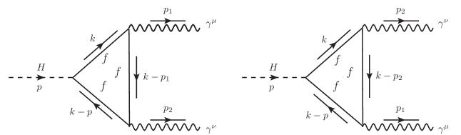
Figure 1: Fermion loop Feynman diagrams of $H\rightarrow\gamma\gamma$ in $R_{\xi}$ gauge.

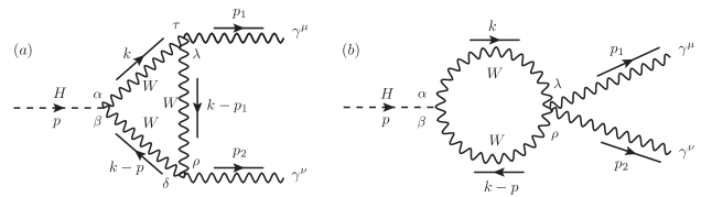
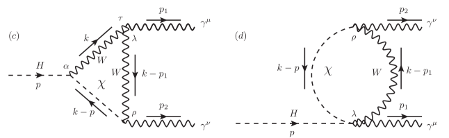
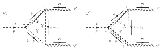
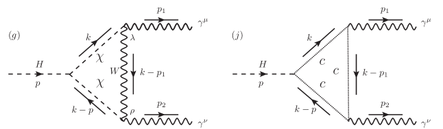
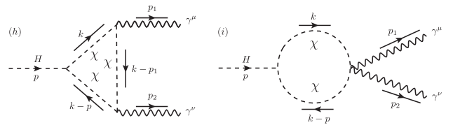
Figure 2: $W$ boson, Goldstone boson, Ghost particles exchanging in the loop diagrams of $H\rightarrow\gamma\gamma$ in $R_{\xi}$ gauge.

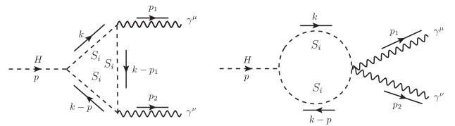
Figure 3: Charged scalar $S_{i}$ exchanged in one-loop Feynman diagrams of $H\rightarrow\gamma\gamma$ in $R_{\xi}$ gauge.

In general, the total amplitude of the decay $H\rightarrow\gamma^{*}\gamma^{*}$ is presented in terms of the Lorentz invariant structure as follows:

$$\mathcal{A}_{H\rightarrow\gamma^{*}\gamma^{*}}=\frac{e^{2}g}{16\pi^{2}M_{W}}\Big{(}\mathcal{A}_{00}g^{\mu\nu}+\sum\limits_{i,j=1}^{2}\mathcal{A}_{ij}p_{i}^{\mu}p_{j}^{\nu}\Big{)}\epsilon_{\mu}^{*}(p_{1})\epsilon_{\nu}^{*}(p_{2}).$$ (12)

The kinematic invariant variables involving the decay channel are

$$p^{2}=(p_{1}+p_{2})^{2}=M_{H}^{2},\quad p_{1}^{2}\quad\text{and}\quad p_{2}^{2}.$$ (13)

In this paper, the form factors $\mathcal{A}_{00},\mathcal{A}_{ij}$ for $i,j=1,2$ are expressed in terms of Passarino-Veltman functions mentioned in the beginning of this section.

In general $R_{\xi}$ gauge, in order to simplify the calculations, $W$ boson propagator is decomposed into the following form with a short notation $M_{\xi}^{2}=\xi M_{W}^{2}$,

$$\dfrac{-i}{p^{2}-M_{W}^{2}}\Bigg{[}g^{\mu\nu}-(1-\xi)\dfrac{p^{\mu}p^{\nu}}{p^{2}-M_{\xi}^{2}}\Bigg{]}=\dfrac{-i}{p^{2}-M_{W}^{2}}\left(g^{\mu\nu}-\dfrac{k^{\mu}k^{\nu}}{M_{W}^{2}}\right)+\dfrac{-i}{p^{2}-M_{\xi}^{2}}\dfrac{k^{\mu}k^{\nu}}{M_{W}^{2}}.$$ (14)

The first term in the right hand side of this equation is nothing but it is $W$ boson propagator in unitary gauge. While the second term relates to Goldstone boson and Ghost particles.

The calculations are performed with the help of Package-X [29] for handling all Dirac traces in $d$ dimensions. The one-loop form factors are then written in terms of Passarino-Veltman functions in standard notations of LoopTools [30] on a diagram-by-diagram basis.

2.1 Two off-shell photons

We first present analytic results for one-loop form factors for the decay $H\rightarrow\gamma^{*}\gamma^{*}$. The notation $\gamma^{*}$ is to one off-shell (or a virtual photon). We arrive at the contribution of fermion loop diagrams. Analytic formulas for the form factors are written in terms of Passarino-Veltman functions as

$$\mathcal{A}_{00}^{(f)} = -4m_{f}^{2}N_{C}Q_{f}^{2}\Big{\{}\mathbf{B}_{0}\left(M_{H}^{2};m_{f}^{2},m_{f}^{2}\right)-4\mathbf{C}_{00}\left(M_{H}^{2},p_{1}^{2},p_{2}^{2};m_{f}^{2},m_{f}^{2},m_{f}^{2}\right)$$ (15)

$$+\dfrac{M_{H}^{2}-p_{1}^{2}-p_{2}^{2}}{2}\;\mathbf{C}_{0}\left(M_{H}^{2},p_{1}^{2},p_{2}^{2};m_{f}^{2},m_{f}^{2},m_{f}^{2}\right)\Big{\}},$$

$$\mathcal{A}_{11}^{(f)} = 8m_{f}^{2}N_{C}Q_{f}^{2}\Big{\{}2\mathbf{C}_{11}\left(M_{H}^{2},p_{1}^{2},p_{2}^{2};m_{f}^{2},m_{f}^{2},m_{f}^{2}\right)+\mathbf{C}_{1}\left(M_{H}^{2},p_{1}^{2},p_{2}^{2};m_{f}^{2},m_{f}^{2},m_{f}^{2}\right)\Big{\}},$$ (16)

$$\mathcal{A}_{12}^{(f)} = 4m_{f}^{2}N_{C}Q_{f}^{2}\Big{\{}4\mathbf{C}_{12}\left(M_{H}^{2},p_{1}^{2},p_{2}^{2};m_{f}^{2},m_{f}^{2},m_{f}^{2}\right)+4\mathbf{C}_{11}\left(M_{H}^{2},p_{1}^{2},p_{2}^{2};m_{f}^{2},m_{f}^{2},m_{f}^{2}\right)$$ (17)

$$+4\mathbf{C}_{1}\left(M_{H}^{2},p_{1}^{2},p_{2}^{2};m_{f}^{2},m_{f}^{2},m_{f}^{2}\right)+2\mathbf{C}_{2}\left(M_{H}^{2},p_{1}^{2},p_{2}^{2};m_{f}^{2},m_{f}^{2},m_{f}^{2}\right)$$

$$+\mathbf{C}_{0}\left(M_{H}^{2},p_{1}^{2},p_{2}^{2};m_{f}^{2},m_{f}^{2},m_{f}^{2}\right)\Big{\}},$$

$$\mathcal{A}_{21}^{(f)} = 4m_{f}^{2}N_{C}Q_{f}^{2}\Big{\{}4\mathbf{C}_{12}\left(M_{H}^{2},p_{1}^{2},p_{2}^{2};m_{f}^{2},m_{f}^{2},m_{f}^{2}\right)+4\mathbf{C}_{11}\left(M_{H}^{2},p_{1}^{2},p_{2}^{2};m_{f}^{2},m_{f}^{2},m_{f}^{2}\right)$$ (18)

$$+4\mathbf{C}_{1}\left(M_{H}^{2},p_{1}^{2},p_{2}^{2};m_{f}^{2},m_{f}^{2},m_{f}^{2}\right)+\mathbf{C}_{0}\left(M_{H}^{2},p_{1}^{2},p_{2}^{2};m_{f}^{2},m_{f}^{2},m_{f}^{2}\right)\Big{\}},$$

$$\mathcal{A}_{22}^{(f)} = 8m_{f}^{2}N_{C}Q_{f}^{2}\Big{\{}2\mathbf{C}_{22}\left(M_{H}^{2},p_{1}^{2},p_{2}^{2};m_{f}^{2},m_{f}^{2},m_{f}^{2}\right)+4\mathbf{C}_{12}\left(M_{H}^{2},p_{1}^{2},p_{2}^{2};m_{f}^{2},m_{f}^{2},m_{f}^{2}\right)$$ (19)

$$+2\mathbf{C}_{11}\left(M_{H}^{2},p_{1}^{2},p_{2}^{2};m_{f}^{2},m_{f}^{2},m_{f}^{2}\right)+\mathbf{C}_{0}\left(M_{H}^{2},p_{1}^{2},p_{2}^{2};m_{f}^{2},m_{f}^{2},m_{f}^{2}\right)$$

$$+3\mathbf{C}_{2}\left(M_{H}^{2},p_{1}^{2},p_{2}^{2};m_{f}^{2},m_{f}^{2},m_{f}^{2}\right)+3\mathbf{C}_{1}\left(M_{H}^{2},p_{1}^{2},p_{2}^{2};m_{f}^{2},m_{f}^{2},m_{f}^{2}\right)\Big{\}}.$$

Here $N_{C}$ is a color factor ($N_{C}=1$ for leptons and $N_{C}=3$ for quarks) and $Q_{f}e$ is electric charge of fermions.

We next consider $W$ boson contributions for the form factors. In general $R_{\xi}$ gauge, the contributions are included $W$ boson, Goldstone boson and Ghost particles in one-loop diagrams. Summing all these diagrams, we get the form factors which are functions of the unphysical parameter $\xi$ and the kinematic invariants $p_{1}^{2},p_{2}^{2},M_{H}^{2},M_{W}^{2}$. For illustrating, we only show here the results in ’t Hooft-Veltman gauge:

$$\mathcal{A}_{00}^{(W)} = M_{W}^{2}\Big{\{}-\mathbf{B}_{0}\left(p_{1}^{2};M_{W}^{2},M_{W}^{2}\right)+\mathbf{B}_{0}\left(p_{2}^{2};M_{W}^{2},M_{W}^{2}\right)$$

$$+2\left(-4M_{H}^{2}+p_{1}^{2}+4p_{2}^{2}\right)\mathbf{C}_{0}\left(p_{1}^{2},p_{2}^{2},M_{H}^{2};M_{W}^{2},M_{W}^{2},M_{W}^{2}\right)\Big{\}}$$

$$-\left[M_{H}^{2}+2(d-1)M_{W}^{2}\right]\times$$

$$\times\Big{\{}\mathbf{B}_{0}\left(M_{H}^{2};M_{W}^{2},M_{W}^{2}\right)-4\mathbf{C}_{00}\left(p_{1}^{2},p_{2}^{2},M_{H}^{2};M_{W}^{2},M_{W}^{2},M_{W}^{2}\right)\Big{\}},$$

$$\mathcal{A}_{11}^{(W)} = 2\left[M_{H}^{2}+2(d+2)M_{W}^{2}\right]\mathbf{C}_{0}\left(p_{1}^{2},p_{2}^{2},M_{H}^{2};M_{W}^{2},M_{W}^{2},M_{W}^{2}\right)$$ (21)

$$+2\left[3M_{H}^{2}+(6d-1)M_{W}^{2}\right]\Big{\{}\mathbf{C}_{2}\left(p_{1}^{2},p_{2}^{2},M_{H}^{2};M_{W}^{2},M_{W}^{2},M_{W}^{2}\right)$$

$$+\mathbf{C}_{1}\left(p_{1}^{2},p_{2}^{2},M_{H}^{2};M_{W}^{2},M_{W}^{2},M_{W}^{2}\right)\Big{\}}$$

$$+4\left[M_{H}^{2}+2(d-1)M_{W}^{2}\right]\Big{\{}\mathbf{C}_{11}\left(p_{1}^{2},p_{2}^{2},M_{H}^{2};M_{W}^{2},M_{W}^{2},M_{W}^{2}\right)$$

$$+\mathbf{C}_{22}\left(p_{1}^{2},p_{2}^{2},M_{H}^{2};M_{W}^{2},M_{W}^{2},M_{W}^{2}\right)+2\mathbf{C}_{12}\left(p_{1}^{2},p_{2}^{2},M_{H}^{2};M_{W}^{2},M_{W}^{2},M_{W}^{2}\right)\Big{\}},$$

$$\mathcal{A}_{12}^{(W)} = 4\left[M_{H}^{2}+2(d-1)M_{W}^{2}\right]\times$$ (22)

$$\times\Big{[}\mathbf{C}_{22}\left(p_{1}^{2},p_{2}^{2},M_{H}^{2};M_{W}^{2},M_{W}^{2},M_{W}^{2}\right)+\mathbf{C}_{12}\left(p_{1}^{2},p_{2}^{2},M_{H}^{2};M_{W}^{2},M_{W}^{2},M_{W}^{2}\right)\Big{]}$$

$$+2\left[M_{H}^{2}+2dM_{W}^{2}\right]$$

$$\times\Big{[}2\mathbf{C}_{2}\left(p_{1}^{2},p_{2}^{2},M_{H}^{2};M_{W}^{2},M_{W}^{2},M_{W}^{2}\right)+\mathbf{C}_{1}\left(p_{1}^{2},p_{2}^{2},M_{H}^{2};M_{W}^{2},M_{W}^{2},M_{W}^{2}\right)\Big{]}$$

$$+\left[M_{H}^{2}+2(d+1)M_{W}^{2}\right]\mathbf{C}_{0}\left(p_{1}^{2},p_{2}^{2},M_{H}^{2};M_{W}^{2},M_{W}^{2},M_{W}^{2}\right),$$

$$\mathcal{A}_{21}^{(W)} = 2M_{W}^{2}\Big{\{}4(d-1)\Big{[}\mathbf{C}_{22}\left(p_{1}^{2},p_{2}^{2},M_{H}^{2};M_{W}^{2},M_{W}^{2},M_{W}^{2}\right)$$ (23)

$$+\mathbf{C}_{12}\left(p_{1}^{2},p_{2}^{2},M_{H}^{2};M_{W}^{2},M_{W}^{2},M_{W}^{2}\right)\Big{]}$$

$$+(4d+2)\mathbf{C}_{2}\left(p_{1}^{2},p_{2}^{2},M_{H}^{2};M_{W}^{2},M_{W}^{2},M_{W}^{2}\right)+11\mathbf{C}_{0}\left(p_{1}^{2},p_{2}^{2},M_{H}^{2};M_{W}^{2},M_{W}^{2},M_{W}^{2}\right)$$

$$+3\mathbf{C}_{1}\left(p_{1}^{2},p_{2}^{2},M_{H}^{2};M_{W}^{2},M_{W}^{2},M_{W}^{2}\right)\Big{\}}+4M_{H}^{2}\Big{\{}\mathbf{C}_{22}\left(p_{1}^{2},p_{2}^{2},M_{H}^{2};M_{W}^{2},M_{W}^{2},M_{W}^{2}\right)$$

$$+\mathbf{C}_{12}\left(p_{1}^{2},p_{2}^{2},M_{H}^{2};M_{W}^{2},M_{W}^{2},M_{W}^{2}\right)+\mathbf{C}_{2}\left(p_{1}^{2},p_{2}^{2},M_{H}^{2};M_{W}^{2},M_{W}^{2},M_{W}^{2}\right)\Big{\}},$$

$$\mathcal{A}_{22}^{(W)} = 4\left[M_{H}^{2}+2(d-1)M_{W}^{2}\right]\mathbf{C}_{22}\left(p_{1}^{2},p_{2}^{2},M_{H}^{2};M_{W}^{2},M_{W}^{2},M_{W}^{2}\right)$$ (24)

$$+2\left[M_{H}^{2}+(2d+3)M_{W}^{2}\right]\mathbf{C}_{2}\left(p_{1}^{2},p_{2}^{2},M_{H}^{2};M_{W}^{2},M_{W}^{2},M_{W}^{2}\right)$$

$$+4M_{W}^{2}\mathbf{C}_{0}\left(p_{1}^{2},p_{2}^{2},M_{H}^{2};M_{W}^{2},M_{W}^{2},M_{W}^{2}\right).$$

We extend our calculation with considering the charged scalar particles $S_{i}$ exchanged in one-loop diagrams. The amplitude for $H\rightarrow\gamma^{*}\gamma^{*}$ with exchanging the charged scalar particles in loop diagrams are decomposed

$$\mathcal{A}_{H\rightarrow\gamma\gamma}^{(S_{i})}=\frac{\lambda_{HS_{i}S_{i}}e^{2}Q_{S_{i}}^{2}}{16\pi^{2}}\Big{(}\mathcal{A}_{00}^{(S_{i})}g^{\mu\nu}+\sum\limits_{i,j=1}^{2}\mathcal{A}_{ij}^{(S_{i})}p_{i}^{\mu}p_{j}^{\nu}\Big{)}\epsilon_{\mu}^{*}(p_{1})\epsilon_{\nu}^{*}(p_{2}).$$ (25)

Applying the same procedure, we derive one-loop form factors due to the contributions of the charged scalar loop diagrams as follows:

$$\mathcal{A}^{(S_{i})}_{00} = -2\Big{\{}\mathbf{B}_{0}\left(M_{H}^{2};M_{S_{i}}^{2},M_{S_{i}}^{2}\right)-4\mathbf{C}_{00}\left(M_{H}^{2},p_{1}^{2},p_{2}^{2};M_{S_{i}}^{2},M_{S_{i}}^{2},M_{S_{i}}^{2}\right)\Big{\}},$$ (26)

$$\mathcal{A}^{(S_{i})}_{11} = 4\Big{\{}2\mathbf{C}_{11}\left(M_{H}^{2},p_{1}^{2},p_{2}^{2};M_{S_{i}}^{2},M_{S_{i}}^{2},M_{S_{i}}^{2}\right)+\mathbf{C}_{1}\left(M_{H}^{2},p_{1}^{2},p_{2}^{2};M_{S_{i}}^{2},M_{S_{i}}^{2},M_{S_{i}}^{2}\right)\Big{\}},$$ (27)

$$\mathcal{A}^{(S_{i})}_{12} = 2\Big{\{}4\mathbf{C}_{12}\left(M_{H}^{2},p_{1}^{2},p_{2}^{2};M_{S_{i}}^{2},M_{S_{i}}^{2},M_{S_{i}}^{2}\right)+4\mathbf{C}_{11}\left(M_{H}^{2},p_{1}^{2},p_{2}^{2};M_{S_{i}}^{2},M_{S_{i}}^{2},M_{S_{i}}^{2}\right)$$ (28)

$$+4\mathbf{C}_{1}\left(M_{H}^{2},p_{1}^{2},p_{2}^{2};M_{S_{i}}^{2},M_{S_{i}}^{2},M_{S_{i}}^{2}\right)+2\mathbf{C}_{2}\left(M_{H}^{2},p_{1}^{2},p_{2}^{2};M_{S_{i}}^{2},M_{S_{i}}^{2},M_{S_{i}}^{2}\right)$$

$$+\mathbf{C}_{0}\left(M_{H}^{2},p_{1}^{2},p_{2}^{2};M_{S_{i}}^{2},M_{S_{i}}^{2},M_{S_{i}}^{2}\right)\Big{\}}$$

and

$$\mathcal{A}^{(S_{i})}_{21} = 8\Big{\{}\mathbf{C}_{12}\left(M_{H}^{2},p_{1}^{2},p_{2}^{2};M_{S_{i}}^{2},M_{S_{i}}^{2},M_{S_{i}}^{2}\right)+\mathbf{C}_{11}\left(M_{H}^{2},p_{1}^{2},p_{2}^{2};M_{S_{i}}^{2},M_{S_{i}}^{2},M_{S_{i}}^{2}\right)$$ (29)

$$+\mathbf{C}_{1}\left(M_{H}^{2},p_{1}^{2},p_{2}^{2};M_{S_{i}}^{2},M_{S_{i}}^{2},M_{S_{i}}^{2}\right)\Big{\}},$$

$$\mathcal{A}^{(S_{i})}_{22} = 4\Big{\{}2\mathbf{C}_{22}\left(M_{H}^{2},p_{1}^{2},p_{2}^{2};M_{S_{i}}^{2},M_{S_{i}}^{2},M_{S_{i}}^{2}\right)+4\mathbf{C}_{12}\left(M_{H}^{2},p_{1}^{2},p_{2}^{2};M_{S_{i}}^{2},M_{S_{i}}^{2},M_{S_{i}}^{2}\right)$$ (30)

$$+2\mathbf{C}_{11}\left(M_{H}^{2},p_{1}^{2},p_{2}^{2};M_{S_{i}}^{2},M_{S_{i}}^{2},M_{S_{i}}^{2}\right)+\mathbf{C}_{0}\left(M_{H}^{2},p_{1}^{2},p_{2}^{2};M_{S_{i}}^{2},M_{S_{i}}^{2},M_{S_{i}}^{2}\right)$$

$$+3\mathbf{C}_{2}\left(M_{H}^{2},p_{1}^{2},p_{2}^{2};M_{S_{i}}^{2},M_{S_{i}}^{2},M_{S_{i}}^{2}\right)+3\mathbf{C}_{1}\left(M_{H}^{2},p_{1}^{2},p_{2}^{2};M_{S_{i}}^{2},M_{S_{i}}^{2},M_{S_{i}}^{2}\right)\Big{\}}.$$

By taking the limit of $p_{1}^{2}\rightarrow 0$ or $p_{2}^{2}\rightarrow 0$, we get the results for the case of one off-shell photon. We refer analytic results for all form factors in which $\gamma(p_{1})$ is on-shell photon in appendix $A$.

2.2 Two on-shell photons

We change our topic to the case of two real photons in the final state of this channel. In this case, on-shell conditions for these photons are implied as

$$p_{1}^{2}=p_{2}^{2}=0.$$ (31)

We then have the relation $p_{1}p_{2}=M_{H}^{2}/2$. On the other hand, Ward identities are taken into account for both photons

$$p_{1}^{\mu}\epsilon^{*}_{\mu}(p_{1})=p_{2}^{\nu}\epsilon^{*}_{\nu}(p_{2})=0.$$ (32)

Subsequently, all form factors

$$\mathcal{A}_{11}=\mathcal{A}_{12}=\mathcal{A}_{22}=0.$$ (33)

Analytic formulas for the remaining form factors are derived as:

$$\mathcal{A}_{00}^{(f)} = -2m_{f}^{2}N_{C}Q_{f}^{2}\Big{\{}2\mathbf{B}_{0}\left(M_{H}^{2};m_{f}^{2},m_{f}^{2}\right)-8\mathbf{C}_{00}\left(M_{H}^{2},0,0;m_{f}^{2},m_{f}^{2},m_{f}^{2}\right)$$ (34)

$$+M_{H}^{2}\mathbf{C}_{0}\left(M_{H}^{2},0,0;m_{f}^{2},m_{f}^{2},m_{f}^{2}\right)\Big{\}},$$

$$\mathcal{A}_{21}^{(f)} = 4m_{f}^{2}N_{C}Q_{f}^{2}\Big{\{}4\Big{[}\mathbf{C}_{12}\left(M_{H}^{2},0,0;m_{f}^{2},m_{f}^{2},m_{f}^{2}\right)+\mathbf{C}_{11}\left(M_{H}^{2},0,0;m_{f}^{2},m_{f}^{2},m_{f}^{2}\right)$$ (35)

$$+\mathbf{C}_{1}\left(M_{H}^{2},0,0;m_{f}^{2},m_{f}^{2},m_{f}^{2}\right)\Big{]}+\mathbf{C}_{0}\left(M_{H}^{2},0,0;m_{f}^{2},m_{f}^{2},m_{f}^{2}\right)\Big{\}}.$$

From one-loop $W$ boson contributions, the analytical results in both ’t Hooft-Veltman and general $R_{\xi}$ gauges are shown. First, the form factors in $R_{\xi}$ gauge read

$$\mathcal{A}^{(W)}_{00}(\xi) = \Big{[}2M_{W}^{2}(1-d)-2M_{H}^{2}-\dfrac{M_{H}^{4}}{2M_{W}^{2}}\Big{]}\mathbf{B}_{0}(M_{H}^{2};M_{W}^{2},M_{W}^{2})$$

$$+\Big{[}\dfrac{M_{H}^{4}}{M_{W}^{2}}+M_{H}^{2}(1-\xi)\Big{]}\mathbf{B}_{0}(M_{H}^{2};M_{\xi}^{2},M_{W}^{2})$$

$$-\Big{(}\dfrac{M_{H}^{4}}{M_{W}^{2}}+2M_{H}^{2}\Big{)}\mathbf{B}_{1}(M_{H}^{2};M_{W}^{2},M_{W}^{2})$$

$$+\Big{(}M_{H}^{2}\xi-\dfrac{M_{H}^{4}}{2M_{W}^{2}}\Big{)}\Big{[}2\mathbf{B}_{1}+\mathbf{B}_{0}\Big{]}(M_{H}^{2};M_{\xi}^{2},M_{\xi}^{2})$$

$$+\Big{[}\dfrac{M_{H}^{4}}{M_{W}^{2}}+M_{H}^{2}(1-\xi)\Big{]}\Big{[}\mathbf{B}_{1}(M_{H}^{2};M_{W}^{2},M_{\xi}^{2})+\mathbf{B}_{1}(M_{H}^{2};M_{\xi}^{2},M_{W}^{2})\Big{]}$$

$$+[4M_{H}^{2}+8M_{W}^{2}(d-1)]\mathbf{C}_{00}(0,0,M_{H}^{2};M_{W}^{2},M_{W}^{2},M_{W}^{2})$$

$$+\Big{[}M_{H}^{2}+M_{W}^{2}(1-\xi)\Big{]}\times$$

$$\times\Big{[}2\mathbf{C}_{00}(0,0,M_{H}^{2};M_{W}^{2},M_{W}^{2},M_{\xi}^{2})-2\mathbf{C}_{00}(0,0,M_{H}^{2};M_{\xi}^{2},M_{W}^{2},M_{W}^{2})$$

$$+\mathbf{C}_{00}(0,0,M_{H}^{2};M_{W}^{2},M_{\xi}^{2},M_{\xi}^{2})-\mathbf{C}_{00}(0,0,M_{H}^{2};M_{\xi}^{2},M_{\xi}^{2},M_{W}^{2})\Big{]}$$

$$+2M_{H}^{2}M_{W}^{2}\Big{[}\mathbf{C}_{0}(0,0,M_{H}^{2};M_{\xi}^{2},M_{W}^{2},M_{W}^{2})$$

$$-\mathbf{C}_{0}(0,0,M_{H}^{2};M_{W}^{2},M_{W}^{2},M_{\xi}^{2})-4\mathbf{C}_{0}(0,0,M_{H}^{2};M_{W}^{2},M_{W}^{2},M_{W}^{2})\Big{]},$$

$$\mathcal{A}^{(W)}_{21}(\xi) = (4M_{H}^{2}+8dM_{W}^{2}-8M_{W}^{2})\Big{[}\mathbf{C}_{22}+\mathbf{C}_{12}+\mathbf{C}_{2}\Big{]}(0,0,M_{H}^{2};M_{W}^{2},M_{W}^{2},M_{W}^{2})$$

$$+\Big{[}M_{H}^{2}+M_{W}^{2}(1-\xi)\Big{]}\times$$

$$\times\Big{[}2\mathbf{C}_{22}(0,0,M_{H}^{2};M_{W}^{2},M_{W}^{2},M_{\xi}^{2})-2\mathbf{C}_{22}(0,0,M_{H}^{2};M_{\xi}^{2},M_{W}^{2},M_{W}^{2})$$

$$+2\mathbf{C}_{12}(0,0,M_{H}^{2};M_{W}^{2},M_{W}^{2},M_{\xi}^{2})-2\mathbf{C}_{12}(0,0,M_{H}^{2};M_{\xi}^{2},M_{W}^{2},M_{W}^{2})$$

$$+\mathbf{C}_{22}(0,0,M_{H}^{2};M_{W}^{2},M_{\xi}^{2},M_{\xi}^{2})-\mathbf{C}_{22}(0,0,M_{H}^{2};M_{\xi}^{2},M_{\xi}^{2},M_{W}^{2})$$

$$+\mathbf{C}_{12}(0,0,M_{H}^{2};M_{W}^{2},M_{\xi}^{2},M_{\xi}^{2})-\mathbf{C}_{12}(0,0,M_{H}^{2};M_{\xi}^{2},M_{\xi}^{2},M_{W}^{2})\Big{]}$$

$$+2M_{W}^{2}\Big{[}2\mathbf{C}_{1}(0,0,M_{H}^{2};M_{\xi}^{2},M_{W}^{2},M_{W}^{2})+\mathbf{C}_{1}(0,0,M_{H}^{2};M_{W}^{2},M_{\xi}^{2},M_{\xi}^{2})$$

$$+2\mathbf{C}_{0}(0,0,M_{H}^{2};M_{W}^{2},M_{W}^{2},M_{\xi}^{2})+\mathbf{C}_{0}(0,0,M_{H}^{2};M_{W}^{2},M_{\xi}^{2},M_{\xi}^{2})\Big{]}$$

$$+\Big{[}M_{H}^{2}+M_{W}^{2}(3-\xi)\Big{]}\times$$

$$\times\Big{[}2\mathbf{C}_{2}(0,0,M_{H}^{2};M_{W}^{2},M_{W}^{2},M_{\xi}^{2})+\mathbf{C}_{2}(0,0,M_{H}^{2};M_{W}^{2},M_{\xi}^{2},M_{\xi}^{2})\Big{]}$$

$$+\Big{[}M_{W}^{2}(1+\xi)-M_{H}^{2}\Big{]}\times$$

$$\times\Big{[}2\mathbf{C}_{2}(0,0,M_{H}^{2};M_{\xi}^{2},M_{W}^{2},M_{W}^{2})+\mathbf{C}_{2}(0,0,M_{H}^{2};M_{\xi}^{2},M_{\xi}^{2},M_{W}^{2})\Big{]}$$

$$+16M_{W}^{2}\mathbf{C}_{0}(0,0,M_{H}^{2};M_{W}^{2},M_{W}^{2},M_{W}^{2})$$

By setting $\xi=1$, we obtain the results in ’t Hooft-Veltman gauge

$$\mathcal{A}_{00}^{(W)} = -\left[M_{H}^{2}+2(d-1)M_{W}^{2}\right]\Big{[}\mathbf{B}_{0}\left(M_{H}^{2};M_{W}^{2},M_{W}^{2}\right)-4\mathbf{C}_{00}\left(0,0,M_{H}^{2};M_{W}^{2},M_{W}^{2},M_{W}^{2}\right)\Big{]}$$ (38)

$$-8M_{H}^{2}M_{W}^{2}\mathbf{C}_{0}\left(0,0,M_{H}^{2};M_{W}^{2},M_{W}^{2},M_{W}^{2}\right),$$

$$\mathcal{A}_{21}^{(W)} = 2M_{W}^{2}\Big{\{}4(d-1)\Big{[}\mathbf{C}_{22}\left(0,0,M_{H}^{2};M_{W}^{2},M_{W}^{2},M_{W}^{2}\right)+\mathbf{C}_{12}\left(0,0,M_{H}^{2};M_{W}^{2},M_{W}^{2},M_{W}^{2}\right)\Big{]}$$ (39)

$$+2(2d+1)\mathbf{C}_{2}\left(0,0,M_{H}^{2};M_{W}^{2},M_{W}^{2},M_{W}^{2}\right)+11\mathbf{C}_{0}\left(0,0,M_{H}^{2};M_{W}^{2},M_{W}^{2},M_{W}^{2}\right)$$

$$+3\mathbf{C}_{1}\left(0,0,M_{H}^{2};M_{W}^{2},M_{W}^{2},M_{W}^{2}\right)\Big{\}}+4M_{H}^{2}\Big{[}\mathbf{C}_{22}\left(0,0,M_{H}^{2};M_{W}^{2},M_{W}^{2},M_{W}^{2}\right)$$

$$+\mathbf{C}_{12}\left(0,0,M_{H}^{2};M_{W}^{2},M_{W}^{2},M_{W}^{2}\right)+\mathbf{C}_{2}\left(0,0,M_{H}^{2};M_{W}^{2},M_{W}^{2},M_{W}^{2}\right)\Big{]}.$$

One-loop form factors for this process with including charged scalars in the loop diagrams are shown

$$\mathcal{A}^{(S_{i})}_{00} = -2\Big{\{}\mathbf{B}_{0}\left(M_{H}^{2};M_{S_{i}}^{2},M_{S_{i}}^{2}\right)-4\mathbf{C}_{00}\left(M_{H}^{2},0,0;M_{S_{i}}^{2},M_{S_{i}}^{2},M_{S_{i}}^{2}\right)\Big{\}},$$ (40)

$$\mathcal{A}^{(S_{i})}_{21} = 8\Big{\{}\mathbf{C}_{12}\left(M_{H}^{2},0,0;M_{S_{i}}^{2},M_{S_{i}}^{2},M_{S_{i}}^{2}\right)+\mathbf{C}_{11}\left(M_{H}^{2},0,0;M_{S_{i}}^{2},M_{S_{i}}^{2},M_{S_{i}}^{2}\right)$$ (41)

$$+\mathbf{C}_{1}\left(M_{H}^{2},0,0;M_{S_{i}}^{2},M_{S_{i}}^{2},M_{S_{i}}^{2}\right)\Big{\}}.$$

We find that all form factors in $R_{\xi=1}$ in two on-shell photons case can be obtained by taking $p_{1}^{2},p_{2}^{2}\rightarrow 0$ from the results in previous subsection.

In the limit of $d\rightarrow 4$, we confirm previous results, taking Ref. [18] as an example. In detail, our results when $d\rightarrow 4$ are presented

$$\mathcal{A}^{(f)}_{00} = \mathcal{A}^{(f)}_{21}\times\left(-\dfrac{M_{H}^{2}}{2}\right)=$$

$$= \frac{m_{f}^{2}N_{C}Q_{f}^{2}}{M_{H}^{2}}\left\{4M_{H}^{2}+\left(4m_{f}^{2}-M_{H}^{2}\right)\ln^{2}\left(\dfrac{-M_{H}^{2}+2m_{f}^{2}+\sqrt{M_{H}^{4}-4m_{f}^{2}M_{H}^{2}}}{2m_{f}^{2}}\right)\right\}$$

and

$$\mathcal{A}^{(W)}_{00} = \mathcal{A}^{(W)}_{21}\times\left(-\dfrac{M_{H}^{2}}{2}\right)=$$

$$= M_{H}^{2}+6M_{W}^{2}+\left(\frac{6M_{W}^{4}}{M_{H}^{2}}-3M_{W}^{2}\right)\ \ln^{2}\left(\frac{-M_{H}^{2}+2M_{W}^{2}+\sqrt{M_{H}^{4}-4M_{H}^{2}M_{W}^{2}}}{2M_{W}^{2}}\right).$$

These results agree with Ref. [18].

Furthermore, we also have analytic results for the form factors due to the charged scalar in the loop at $d=4$. These factors read

$$\mathcal{A}^{(S_{i})}_{00} = \mathcal{A}^{(S_{i})}_{21}\times\left(-\dfrac{M_{H}^{2}}{2}\right)=$$

$$= \frac{2\lambda_{HS_{i}S_{i}}M_{W}Q_{S_{i}}^{2}}{gM_{H}^{2}}\left\{M_{H}^{2}+M_{S_{i}}^{2}\ln^{2}\left(\frac{-M_{H}^{2}+2M_{S_{i}}^{2}+\sqrt{M_{H}^{4}-4M_{H}^{2}M_{S_{i}}^{2}}}{2M_{S_{i}}^{2}}\right)\right\}.$$

The $\xi$-independent of the result is also discussed. The numerical results are generated by varying $\xi\rightarrow 0$ (is so-called Coulomb gauge), $\xi=1$ or ’t Hooft-Veltman gauge and $\xi\rightarrow\infty$ ( unitary gauge). In this Table 1, we show the numerical results of

$$(-2/M_{H}^{2})\times\mathcal{A}_{00}=\mathcal{A}_{21}.$$ (45)

We find that numerical results are good stability in different gauges.

$\textbf{diagrams}/\xi$	$\xi\rightarrow 0$	$\xi=1$	$\xi=100$	$\xi\rightarrow\infty$
$a$	$-3.468876070276491$	$-4.882018101498933$	$-30.40120343875694$	$-2.777777777516398\cdot 10^{11}$
	$+0.044696724580243\,i$
$b$	$0.4359747855634294$	$0$	$22.87057225068166$	$2.777777777438721\cdot 10^{11}$
	$+1.1775870133864408\,i$
$c$	$-2.288315292217131$	$-2.345059943153266$	$-0.5672364405722673$	$-0.3888888890439217$
	$-0.647907755004331\,i$
$d$	$0$	$0$	$0$	$0$
$e$	$-1.599294975435531$	$-1.591326628583693$	$-0.1930905308944328$	$-0.1666666666694787$
	$-1.787032617316791\,i$
$f$	$0.2615610107425627$	$0$	$0.04694802196574567$	$0.08333333330075746$
	$+0.8935163086583953\,i$
$g$	$0.3357098311660154$	$0$	$0.0003307252303052892$	$3.357186222008115\cdot 10^{-14}$
	$+0.3191403256960426\,i$
$h$	$-2$	$0.6243029825430905$	$0.004041657968703369$	$4.028623466417146\cdot 10^{-13}$
$i$	$0$	$0$	$0$	$0$
$j$	$0$	$-0.12913901976434381$	$-0.08360295607991542$	$-0.08333333333336019$
Sum	$-8.323240710457146$	$-8.323240710457146$	$-8.323240710457146$	$-8.323240710457146$

Table 1: The numerical checks for the form factors in the case of $\xi\rightarrow 0,\xi=1,\xi\rightarrow\infty$ are shown. For this check, we set $M_{H}=125$ GeV, $M_{W}=80.4$ GeV, and $p_{1}^{2}=p_{2}^{2}=0$ GeV.

3 Conclusions

In this paper, we have presented one-loop form factors for $H\rightarrow\gamma^{*}\gamma^{*}$ in $R_{\xi}$ gauge, considering all cases of two on-shell, one on-shell and two off-shell for final photons. The calculations are performed in standard model and in arbitrary beyond the standard models which the charged scalar particles may be exchanged in one-loop diagrams. Analytic results for the form factors are shown in general forms which are expressed in terms of the Passarino-Veltman functions in stadard notation of LoopTools. We have also confirmed the results in previous computations which are available for the case of two on-shell photons. The $\xi$-independent of the result has been also studied. We find that numerical results are good stability with varying $\xi=0,1$ and $\xi\rightarrow\infty$.

Acknowledgment:  This research is funded by Vietnam National Foundation for Science and Technology Development (NAFOSTED) under the grant number $103.01$-$2019.346$.

Appendix A: One-loop form factors for $H\rightarrow\gamma\gamma^{*}$

Analytical results for one off-shell photon in the decay of $H\rightarrow\gamma\gamma^{*}$ are reported in this subsection. Without loss the generality, we consider $\gamma(p_{1})$ is real photon. As a result, we have on-shell condition for $\gamma(p_{1})$ which is $p_{1}^{2}=0$. Following Ward identity, one also has $p_{1}^{\mu}\epsilon^{*}_{\mu}(p_{1})=0$. Subsequently, the form factors $\mathcal{A}_{11}=\mathcal{A}_{12}=0$. Other form factors are given in the following paragraphs. Due to the fermion loop contributions, the form factors are shown

$$\mathcal{A}_{00}^{(f)} = -4m_{f}^{2}N_{C}Q_{f}^{2}\Big{\{}\mathbf{B}_{0}\left(M_{H}^{2};m_{f}^{2},m_{f}^{2}\right)-4\mathbf{C}_{00}\left(M_{H}^{2},0,p_{2}^{2};m_{f}^{2},m_{f}^{2},m_{f}^{2}\right)$$ (46)

$$+\dfrac{M_{H}^{2}-p_{2}^{2}}{2}\mathbf{C}_{0}\left(M_{H}^{2},0,p_{2}^{2};m_{f}^{2},m_{f}^{2},m_{f}^{2}\right)\Big{\}},$$

$$\mathcal{A}_{21}^{(f)} = 4m_{f}^{2}N_{C}Q_{f}^{2}\Big{\{}4\Big{[}\mathbf{C}_{12}\left(M_{H}^{2},0,p_{2}^{2};m_{f}^{2},m_{f}^{2},m_{f}^{2}\right)+\mathbf{C}_{11}\left(M_{H}^{2},0,p_{2}^{2};m_{f}^{2},m_{f}^{2},m_{f}^{2}\right)$$ (47)

$$+\mathbf{C}_{1}\left(M_{H}^{2},0,p_{2}^{2};m_{f}^{2},m_{f}^{2},m_{f}^{2}\right)\Big{]}+\mathbf{C}_{0}\left(M_{H}^{2},0,p_{2}^{2};m_{f}^{2},m_{f}^{2},m_{f}^{2}\right)\Big{\}}$$

$$\mathcal{A}_{22}^{(f)} = 8m_{f}^{2}N_{C}Q_{f}^{2}\Big{\{}2\mathbf{C}_{22}\left(M_{H}^{2},0,p_{2}^{2};m_{f}^{2},m_{f}^{2},m_{f}^{2}\right)+4\mathbf{C}_{12}\left(M_{H}^{2},0,p_{2}^{2};m_{f}^{2},m_{f}^{2},m_{f}^{2}\right)$$ (48)

$$+2\mathbf{C}_{11}\left(M_{H}^{2},0,p_{2}^{2};m_{f}^{2},m_{f}^{2},m_{f}^{2}\right)+\mathbf{C}_{0}\left(M_{H}^{2},0,p_{2}^{2};m_{f}^{2},m_{f}^{2},m_{f}^{2}\right)$$

$$+3\mathbf{C}_{2}\left(M_{H}^{2},0,p_{2}^{2};m_{f}^{2},m_{f}^{2},m_{f}^{2}\right)+3\mathbf{C}_{1}\left(M_{H}^{2},0,p_{2}^{2};m_{f}^{2},m_{f}^{2},m_{f}^{2}\right)\Big{\}}.$$

Applying the same procedure, the form factors calculating from $W$ boson loop diagrams are expressed as follows

$$\mathcal{A}_{00}^{(W)} = M_{W}^{2}\Big{\{}\mathbf{B}_{0}\left(p_{2}^{2};M_{W}^{2},M_{W}^{2}\right)+8\left[p_{2}^{2}-M_{H}^{2}\right]\mathbf{C}_{0}\left(0,p_{2}^{2},M_{H}^{2};M_{W}^{2},M_{W}^{2},M_{W}^{2}\right)\Big{\}}$$ (49)

$$-\left[M_{H}^{2}+2(d-1)M_{W}^{2}\right]\Big{[}\mathbf{B}_{0}\left(M_{H}^{2};M_{W}^{2},M_{W}^{2}\right)-4\mathbf{C}_{00}\left(0,p_{2}^{2},M_{H}^{2};M_{W}^{2},M_{W}^{2},M_{W}^{2}\right)\Big{]}$$

$$-M_{W}^{2}\mathbf{B}_{0}(0;M_{W}^{2},M_{W}^{2})$$

$$\mathcal{A}_{21}^{(W)} = 2M_{W}^{2}\Big{\{}4(d-1)\Big{[}\mathbf{C}_{22}\left(0,p_{2}^{2},M_{H}^{2};M_{W}^{2},M_{W}^{2},M_{W}^{2}\right)+\mathbf{C}_{12}\left(0,p_{2}^{2},M_{H}^{2};M_{W}^{2},M_{W}^{2},M_{W}^{2}\right)\Big{]}$$ (50)

$$+2(2d+1)\mathbf{C}_{2}\left(0,p_{2}^{2},M_{H}^{2};M_{W}^{2},M_{W}^{2},M_{W}^{2}\right)+11\mathbf{C}_{0}\left(0,p_{2}^{2},M_{H}^{2};M_{W}^{2},M_{W}^{2},M_{W}^{2}\right)$$

$$+3\mathbf{C}_{1}\left(0,p_{2}^{2},M_{H}^{2};M_{W}^{2},M_{W}^{2},M_{W}^{2}\right)\Big{\}}+4M_{H}^{2}\Big{\{}\mathbf{C}_{22}\left(0,p_{2}^{2},M_{H}^{2};M_{W}^{2},M_{W}^{2},M_{W}^{2}\right)$$

$$+\mathbf{C}_{12}\left(0,p_{2}^{2},M_{H}^{2};M_{W}^{2},M_{W}^{2},M_{W}^{2}\right)+\mathbf{C}_{2}\left(0,p_{2}^{2},M_{H}^{2};M_{W}^{2},M_{W}^{2},M_{W}^{2}\right)\Big{\}},$$

$$\mathcal{A}_{22}^{(W)} = 4\left[M_{H}^{2}+2(d-1)M_{W}^{2}\right]\mathbf{C}_{22}\left(0,p_{2}^{2},M_{H}^{2};M_{W}^{2},M_{W}^{2},M_{W}^{2}\right)$$ (51)

$$+2\left[M_{H}^{2}+(2d+3)M_{W}^{2}\right]\mathbf{C}_{2}\left(0,p_{2}^{2},M_{H}^{2};M_{W}^{2},M_{W}^{2},M_{W}^{2}\right)$$

$$+4M_{W}^{2}\mathbf{C}_{0}\left(0,p_{2}^{2},M_{H}^{2};M_{W}^{2},M_{W}^{2},M_{W}^{2}\right).$$

Further, one-loop form factors for this channel with contributing of charged scalars in the loop diagrams are obtained

$$\mathcal{A}^{(S_{i})}_{00} = -2\Big{\{}\mathbf{B}_{0}\left(M_{H}^{2};M_{S_{i}}^{2},M_{S_{i}}^{2}\right)-4\mathbf{C}_{00}\left(M_{H}^{2},0,p_{2}^{2};M_{S_{i}}^{2},M_{S_{i}}^{2},M_{S_{i}}^{2}\right)\Big{\}},$$ (52)

$$\mathcal{A}^{(S_{i})}_{21} = 8\Big{\{}\mathbf{C}_{12}\left(M_{H}^{2},0,p_{2}^{2};M_{S_{i}}^{2},M_{S_{i}}^{2},M_{S_{i}}^{2}\right)+\mathbf{C}_{11}\left(M_{H}^{2},0,p_{2}^{2};M_{S_{i}}^{2},M_{S_{i}}^{2},M_{S_{i}}^{2}\right)$$ (53)

$$+\mathbf{C}_{1}\left(M_{H}^{2},0,p_{2}^{2};M_{S_{i}}^{2},M_{S_{i}}^{2},M_{S_{i}}^{2}\right)\Big{\}},$$

$$\mathcal{A}^{(S_{i})}_{22} = 4\Big{\{}2\mathbf{C}_{22}\left(M_{H}^{2},0,p_{2}^{2};M_{S_{i}}^{2},M_{S_{i}}^{2},M_{S_{i}}^{2}\right)+4\mathbf{C}_{12}\left(M_{H}^{2},0,p_{2}^{2};M_{S_{i}}^{2},M_{S_{i}}^{2},M_{S_{i}}^{2}\right)$$ (54)

$$+2\mathbf{C}_{11}\left(M_{H}^{2},0,p_{2}^{2};M_{S_{i}}^{2},M_{S_{i}}^{2},M_{S_{i}}^{2}\right)+\mathbf{C}_{0}\left(M_{H}^{2},0,p_{2}^{2};M_{S_{i}}^{2},M_{S_{i}}^{2},M_{S_{i}}^{2}\right)$$

$$+3\mathbf{C}_{2}\left(M_{H}^{2},0,p_{2}^{2};M_{S_{i}}^{2},M_{S_{i}}^{2},M_{S_{i}}^{2}\right)+3\mathbf{C}_{1}\left(M_{H}^{2},0,p_{2}^{2};M_{S_{i}}^{2},M_{S_{i}}^{2},M_{S_{i}}^{2}\right)\Big{\}}.$$

We find that all form factors in this subsection can be obtained by taking $p_{1}^{2}\rightarrow 0$ from the results in two off-shell photons.

Appendix $B$: Feynman rules for $H\rightarrow\gamma\gamma$ in $R_{\xi}$ gauge

Feynman rules for $H\rightarrow\gamma\gamma$ in $R_{\xi}$ gauge devoted in this appendix.

Particle types	Propagators
Fermions	$\dfrac{i(\not{p}+m_{f})}{p^{2}-m_{f}^{2}}$
$W$ boson	$\dfrac{-i}{p^{2}-M_{W}^{2}}\Bigg{[}g^{\mu\nu}-(1-\xi)\dfrac{p^{\mu}p^{\nu}}{p^{2}-M_{\xi}^{2}}\Bigg{]}$
Goldstone boson	$\dfrac{i}{p^{2}-M_{\xi}^{2}}$
Ghost	$\dfrac{i}{p^{2}-M_{\xi}^{2}}$
Charged scalar	$\dfrac{i}{p^{2}-M_{S_{i}}^{2}}$

Table 2: Feynman rules involving the decay $H\rightarrow\gamma\gamma$ through fermion and $W$ boson, charged scalar loop diagrams in the $R_{\xi}$ gauge.

Vertices	Couplings
$A_{\mu}f\bar{f}$	$ieQ_{f}\gamma_{\mu}$
$Hf\bar{f}$	$-igm_{f}/(2M_{W})$
$H\cdot W_{\mu}\cdot W_{\nu}$	$igM_{W}g_{\mu\nu}$
$A_{\mu}(p_{1})\cdot W^{+}_{\nu}(p_{2})\cdot W^{-}_{\lambda}(p_{3})$	$-ie\Gamma_{\mu\nu\lambda}(p_{1},p_{2},p_{3})$
$A_{\mu}\cdot A_{\nu}\cdot W^{+}_{\alpha}\cdot W^{-}_{\beta}$	$-ie^{2}S_{\mu\nu,\alpha\beta}$
$H(p_{1})\cdot W_{\mu}\cdot\chi(p_{2})$	$-i\dfrac{g}{2}(p_{2}-p_{1})_{\mu}$
$A_{\mu}\cdot W_{\nu}\cdot\chi$	$-ieM_{W}g_{\mu\nu}$
$H\cdot\chi\cdot\chi$	$-igM_{H}^{2}/(2M_{W})$
$A_{\mu}\cdot\chi(p_{1})\cdot\chi(p_{2})$	$-ie(p_{2}-p_{1})_{\mu}$
$A_{\mu}\cdot A_{\nu}\cdot\chi\cdot\chi$	$i2e^{2}g_{\mu\nu}$
$H\cdot A_{\mu}\cdot W_{\nu}\cdot\chi$	$-ie\dfrac{g}{2}g_{\mu\nu}$
$H\cdot c\cdot c$	$-i\xi\dfrac{g}{2}M_{W}$
$A_{\mu}\cdot c\cdot c$	$-iep_{\mu}$
$HS_{i}\bar{S}_{i}$	$i\lambda_{HS_{i}\bar{S}_{i}}$
$A_{\mu}S_{i}(q_{1})\bar{S}_{i}(q_{2})$	$ieQ_{S_{i}}(q_{2}-q_{1})_{\mu}$
$A_{\mu}A_{\nu}S_{i}\bar{S}_{i}$	$2ie^{2}Q_{S_{i}}^{2}g_{\mu\nu}$

Table 3: Couplings involving the decay $H\rightarrow\gamma\gamma$ through fermion and $W$ boson, charged scalar loops in a in $R_{\xi}$ gauge with the short notation for the standard Lorentz tensors of the gauge boson self couplings $\Gamma_{\mu\nu\lambda}(p_{1},p_{2},p_{3})=g_{\mu\nu}(p_{1}-p_{2})_{\lambda}+g_{\lambda\nu}(p_{2}-p_{3})_{\mu}+g_{\mu\lambda}(p_{3}-p_{1})_{\nu}$ and $S_{\mu\nu,\alpha\beta}=2g_{\mu\nu}g_{\alpha\beta}-g_{\mu\alpha}g_{\nu\beta}-g_{\mu\beta}g_{\nu\alpha}$.

Appendix $C$: Amplitude $H\rightarrow\gamma\gamma$ in $R_{\xi}$ gauge

One-loop Feynman amplitudes for the process $H\rightarrow\gamma\gamma$ in $R_{\xi}$ gauge are shown in this appendix. For fermion loop diagrams, one has

$$\mathcal{A}^{(\text{fermion})}_{(1+2)} = \dfrac{gm_{f}Q_{f}^{2}e^{2}}{M_{W}}\int\dfrac{{\rm d}^{d}k}{(2\pi)^{d}}\,\dfrac{\text{Tr}\{(\not{k}+m_{f})\gamma^{\mu}(\not{k}-\not{p_{1}}+m_{f})\gamma^{\nu}(\not{k}-\not{p}+m_{f})\}}{(k^{2}-m_{f}^{2})[(k-p_{1})^{2}-m_{f}^{2}][(k-p)^{2}-m_{f}^{2}]}\varepsilon_{\mu}^{*}(p_{1})\varepsilon_{\nu}^{*}(p_{2}).$$

We next show Feynman amplitude for $W$ boson loop diagrams

Diagram $a$

The Feynman amplitude for $W$ boson loop diagrams are decomposed into $8$ terms as follows:

$$\mathcal{A}^{(a)}(\xi) = \mathcal{A}_{111}(\xi)+\mathcal{A}_{112}(\xi)+\mathcal{A}_{121}(\xi)+\mathcal{A}_{211}(\xi)$$ (56)

$$+\mathcal{A}_{122}(\xi)+\mathcal{A}_{212}(\xi)+\mathcal{A}_{221}(\xi)+\mathcal{A}_{222}(\xi).$$

Where $\mathcal{A}_{111}(\xi),\cdots,\mathcal{A}_{222}(\xi)$ are corresponding to which term in the right hand side of Eq. (14) is taken. These terms are written

$$\mathcal{A}_{111}(\xi) = 2e^{2}gM_{W}\int\dfrac{{\rm d}^{d}k}{(2\pi)^{d}}\,g_{\alpha\beta}\Gamma_{\mu\tau\lambda}(-p_{1},k,-k+p_{1})\Gamma_{\nu\rho\delta}(-p_{2},k-p_{1},-k+p)\,\epsilon_{\mu}^{*}(p_{1})\epsilon_{\nu}^{*}(p_{2})$$ (57)

$$\times\dfrac{g^{\alpha\tau}-k^{\alpha}k^{\tau}/M_{W}^{2}}{k^{2}-M_{W}^{2}}\dfrac{g^{\lambda\rho}-(k-p_{1})^{\lambda}(k-p_{1})^{\rho}/M_{W}^{2}}{(k-p_{1})^{2}-M_{W}^{2}}\dfrac{g^{\beta\delta}-(k-p)^{\beta}(k-p)^{\delta}/M_{W}^{2}}{(k-p)^{2}-M_{W}^{2}},$$

$$\mathcal{A}_{112}(\xi) = 2e^{2}gM_{W}\int\dfrac{{\rm d}^{d}k}{(2\pi)^{d}}\,g_{\alpha\beta}\Gamma_{\mu\tau\lambda}(-p_{1},k,-k+p_{1})\Gamma_{\nu\rho\delta}(-p_{2},k-p_{1},-k+p)\,\epsilon_{\mu}^{*}(p_{1})\epsilon_{\nu}^{*}(p_{2})$$ (58)

$$\times\dfrac{g^{\alpha\tau}-k^{\alpha}k^{\tau}/M_{W}^{2}}{k^{2}-M_{W}^{2}}\dfrac{g^{\lambda\rho}-(k-p_{1})^{\lambda}(k-p_{1})^{\rho}/M_{W}^{2}}{(k-p_{1})^{2}-M_{W}^{2}}\dfrac{(k-p)^{\beta}(k-p)^{\delta}/M_{W}^{2}}{(k-p)^{2}-M_{\xi}^{2}},$$

$$\mathcal{A}_{121}(\xi) = 2e^{2}gM_{W}\int\dfrac{{\rm d}^{d}k}{(2\pi)^{d}}\,g_{\alpha\beta}\Gamma_{\mu\tau\lambda}(-p_{1},k,-k+p_{1})\Gamma_{\nu\rho\delta}(-p_{2},k-p_{1},-k+p)\,\epsilon_{\mu}^{*}(p_{1})\epsilon_{\nu}^{*}(p_{2})$$ (59)

$$\times\dfrac{g^{\alpha\tau}-k^{\alpha}k^{\tau}/M_{W}^{2}}{k^{2}-M_{W}^{2}}\dfrac{(k-p_{1})^{\lambda}(k-p_{1})^{\rho}/M_{W}^{2}}{(k-p_{1})^{2}-M_{\xi}^{2}}\dfrac{g^{\beta\delta}-(k-p)^{\beta}(k-p)^{\delta}/M_{W}^{2}}{(k-p)^{2}-M_{W}^{2}},$$

$$\mathcal{A}_{211}(\xi) = 2e^{2}gM_{W}\int\dfrac{{\rm d}^{d}k}{(2\pi)^{d}}\,g_{\alpha\beta}\Gamma_{\mu\tau\lambda}(-p_{1},k,-k+p_{1})\Gamma_{\nu\rho\delta}(-p_{2},k-p_{1},-k+p)\,\epsilon_{\mu}^{*}(p_{1})\epsilon_{\nu}^{*}(p_{2})$$ (60)

$$\times\dfrac{k^{\alpha}k^{\tau}/M_{W}^{2}}{k^{2}-M_{\xi}^{2}}\dfrac{g^{\lambda\rho}-(k-p_{1})^{\lambda}(k-p_{1})^{\rho}/M_{W}^{2}}{(k-p_{1})^{2}-M_{W}^{2}}\dfrac{g^{\beta\delta}-(k-p)^{\beta}(k-p)^{\delta}/M_{W}^{2}}{(k-p)^{2}-M_{W}^{2}},$$

$$\mathcal{A}_{122}(\xi) = 2e^{2}gM_{W}\int\dfrac{{\rm d}^{d}k}{(2\pi)^{d}}\,g_{\alpha\beta}\Gamma_{\mu\tau\lambda}(-p_{1},k,-k+p_{1})\Gamma_{\nu\rho\delta}(-p_{2},k-p_{1},-k+p)\,\epsilon_{\mu}^{*}(p_{1})\epsilon_{\nu}^{*}(p_{2})$$ (61)

$$\times\dfrac{g^{\alpha\tau}-k^{\alpha}k^{\tau}/M_{W}^{2}}{k^{2}-M_{W}^{2}}\dfrac{(k-p_{1})^{\lambda}(k-p_{1})^{\rho}/M_{W}^{2}}{(k-p_{1})^{2}-M_{\xi}^{2}}\dfrac{(k-p)^{\beta}(k-p)^{\delta}/M_{W}^{2}}{(k-p)^{2}-M_{\xi}^{2}},$$

$$\mathcal{A}_{212}(\xi) = 2e^{2}gM_{W}\int\dfrac{{\rm d}^{d}k}{(2\pi)^{d}}\,g_{\alpha\beta}\Gamma_{\mu\tau\lambda}(-p_{1},k,-k+p_{1})\Gamma_{\nu\rho\delta}(-p_{2},k-p_{1},-k+p)\,\epsilon_{\mu}^{*}(p_{1})\epsilon_{\nu}^{*}(p_{2})$$ (62)

$$\times\dfrac{k^{\alpha}k^{\tau}/M_{W}^{2}}{k^{2}-M_{\xi}^{2}}\dfrac{g^{\lambda\rho}-(k-p_{1})^{\lambda}(k-p_{1})^{\rho}/M_{W}^{2}}{(k-p_{1})^{2}-M_{W}^{2}}\dfrac{(k-p)^{\beta}(k-p)^{\delta}/M_{W}^{2}}{(k-p)^{2}-M_{\xi}^{2}},$$

$$\mathcal{A}_{221}(\xi) = 2e^{2}gM_{W}\int\dfrac{{\rm d}^{d}k}{(2\pi)^{d}}\,g_{\alpha\beta}\Gamma_{\mu\tau\lambda}(-p_{1},k,-k+p_{1})\Gamma_{\nu\rho\delta}(-p_{2},k-p_{1},-k+p)\,\epsilon_{\mu}^{*}(p_{1})\epsilon_{\nu}^{*}(p_{2})$$ (63)

$$\times\dfrac{k^{\alpha}k^{\tau}/M_{W}^{2}}{k^{2}-M_{\xi}^{2}}\dfrac{(k-p_{1})^{\lambda}(k-p_{1})^{\rho}/M_{W}^{2}}{(k-p_{1})^{2}-M_{\xi}^{2}}\dfrac{g^{\beta\delta}-(k-p)^{\beta}(k-p)^{\delta}/M_{W}^{2}}{(k-p)^{2}-M_{W}^{2}},$$

$$\mathcal{A}_{222}(\xi) = 2e^{2}gM_{W}\int\dfrac{{\rm d}^{d}k}{(2\pi)^{d}}\,g_{\alpha\beta}\Gamma_{\mu\tau\lambda}(-p_{1},k,-k+p_{1})\Gamma_{\nu\rho\delta}(-p_{2},k-p_{1},-k+p)\,\epsilon_{\mu}^{*}(p_{1})\epsilon_{\nu}^{*}(p_{2})$$ (64)

$$\times\dfrac{k^{\alpha}k^{\tau}/M_{W}^{2}}{k^{2}-M_{\xi}^{2}}\dfrac{(k-p_{1})^{\lambda}(k-p_{1})^{\rho}/M_{W}^{2}}{(k-p_{1})^{2}-M_{\xi}^{2}}\dfrac{(k-p)^{\beta}(k-p)^{\delta}/M_{W}^{2}}{(k-p)^{2}-M_{\xi}^{2}}.$$

Diagram $b$

$$\mathcal{A}^{(b)}(\xi) = \mathcal{A}_{11}(\xi)+\mathcal{A}_{12}(\xi)+\mathcal{A}_{21}(\xi)+\mathcal{A}_{22}(\xi)$$ (65)

where

$$\mathcal{A}_{11}(\xi) = -e^{2}gM_{W}\int\dfrac{{\rm d}^{d}k}{(2\pi)^{d}}\,g_{\alpha\beta}S_{\mu\nu,\lambda\rho}\,\epsilon_{\mu}^{*}(p_{1})\epsilon_{\nu}^{*}(p_{2})$$ (66)

$$\times\dfrac{g^{\alpha\lambda}-k^{\alpha}k^{\lambda}/M_{W}^{2}}{k^{2}-M_{W}^{2}}\dfrac{g^{\beta\rho}-(k-p)^{\beta}(k-p)^{\rho}/M_{W}^{2}}{(k-p)^{2}-M_{W}^{2}},$$

$$\mathcal{A}_{12}(\xi) = -e^{2}gM_{W}\int\dfrac{{\rm d}^{d}k}{(2\pi)^{d}}\,g_{\alpha\beta}S_{\mu\nu,\lambda\rho}\,\epsilon_{\mu}^{*}(p_{1})\epsilon_{\nu}^{*}(p_{2})$$ (67)

$$\times\dfrac{g^{\alpha\lambda}-k^{\alpha}k^{\lambda}/M_{W}^{2}}{k^{2}-M_{W}^{2}}\dfrac{(k-p)^{\beta}(k-p)^{\rho}/M_{W}^{2}}{(k-p)^{2}-M_{\xi}^{2}},$$

$$\mathcal{A}_{21}(\xi) = -e^{2}gM_{W}\int\dfrac{{\rm d}^{d}k}{(2\pi)^{d}}\,g_{\alpha\beta}S_{\mu\nu,\lambda\rho}\,\epsilon_{\mu}^{*}(p_{1})\epsilon_{\nu}^{*}(p_{2})$$ (68)

$$\times\dfrac{k^{\alpha}k^{\lambda}/M_{W}^{2}}{k^{2}-M_{\xi}^{2}}\dfrac{g^{\beta\rho}-(k-p)^{\beta}(k-p)^{\rho}/M_{W}^{2}}{(k-p)^{2}-M_{W}^{2}},$$

$$\mathcal{A}_{22}(\xi) = -e^{2}gM_{W}\int\dfrac{{\rm d}^{d}k}{(2\pi)^{d}}\,g_{\alpha\beta}S_{\mu\nu,\lambda\rho}\,\epsilon_{\mu}^{*}(p_{1})\epsilon_{\nu}^{*}(p_{2})$$ (69)

$$\times\dfrac{k^{\alpha}k^{\lambda}/M_{W}^{2}}{k^{2}-M_{\xi}^{2}}\dfrac{(k-p)^{\beta}(k-p)^{\rho}/M_{W}^{2}}{(k-p)^{2}-M_{\xi}^{2}}.$$

Diagram $c$

$$\mathcal{A}^{(c)}(\xi) = \mathcal{A}_{110}(\xi)+\mathcal{A}_{120}(\xi)+\mathcal{A}_{210}(\xi)+\mathcal{A}_{220}(\xi)$$ (70)

where

$$\mathcal{A}_{110}(\xi) = 2e^{2}gM_{W}\int\dfrac{{\rm d}^{d}k}{(2\pi)^{d}}\,(k-2p)_{\alpha}g_{\nu\rho}\Gamma_{\mu\tau\lambda}(-p_{1},k,-k+p_{1})\,\epsilon_{\mu}^{*}(p_{1})\epsilon_{\nu}^{*}(p_{2})$$ (71)

$$\times\dfrac{g^{\alpha\tau}-k^{\alpha}k^{\tau}/M_{W}^{2}}{k^{2}-M_{W}^{2}}\dfrac{g^{\lambda\rho}-(k-p_{1})^{\lambda}(k-p_{1})^{\rho}/M_{W}^{2}}{(k-p_{1})^{2}-M_{W}^{2}}\dfrac{1}{(k-p)^{2}-M_{\xi}^{2}},$$

$$\mathcal{A}_{120}(\xi) = 2e^{2}gM_{W}\int\dfrac{{\rm d}^{d}k}{(2\pi)^{d}}\,(k-2p)_{\alpha}g_{\nu\rho}\Gamma_{\mu\tau\lambda}(-p_{1},k,-k+p_{1})\,\epsilon_{\mu}^{*}(p_{1})\epsilon_{\nu}^{*}(p_{2})$$ (72)

$$\times\dfrac{g^{\alpha\tau}-k^{\alpha}k^{\tau}/M_{W}^{2}}{k^{2}-M_{W}^{2}}\dfrac{(k-p_{1})^{\lambda}(k-p_{1})^{\rho}/M_{W}^{2}}{(k-p_{1})^{2}-M_{\xi}^{2}}\dfrac{1}{(k-p)^{2}-M_{\xi}^{2}},$$

$$\mathcal{A}_{210}(\xi) = 2e^{2}gM_{W}\int\dfrac{{\rm d}^{d}k}{(2\pi)^{d}}\,(k-2p)_{\alpha}g_{\nu\rho}\Gamma_{\mu\tau\lambda}(-p_{1},k,-k+p_{1})\,\epsilon_{\mu}^{*}(p_{1})\epsilon_{\nu}^{*}(p_{2})$$ (73)

$$\times\dfrac{k^{\alpha}k^{\tau}/M_{W}^{2}}{k^{2}-M_{\xi}^{2}}\dfrac{g^{\lambda\rho}-(k-p_{1})^{\lambda}(k-p_{1})^{\rho}/M_{W}^{2}}{(k-p_{1})^{2}-M_{W}^{2}}\dfrac{1}{(k-p)^{2}-M_{\xi}^{2}},$$

$$\mathcal{A}_{220}(\xi) = 2e^{2}gM_{W}\int\dfrac{{\rm d}^{d}k}{(2\pi)^{d}}\,(k-2p)_{\alpha}g_{\nu\rho}\Gamma_{\mu\tau\lambda}(-p_{1},k,-k+p_{1})\,\epsilon_{\mu}^{*}(p_{1})\epsilon_{\nu}^{*}(p_{2})$$ (74)

$$\times\dfrac{k^{\alpha}k^{\tau}/M_{W}^{2}}{k^{2}-M_{\xi}^{2}}\dfrac{(k-p_{1})^{\lambda}(k-p_{1})^{\rho}/M_{W}^{2}}{(k-p_{1})^{2}-M_{\xi}^{2}}\dfrac{1}{(k-p)^{2}-M_{\xi}^{2}}.$$

Diagram $d$

$$\mathcal{A}^{(d)}(\xi) = \mathcal{A}_{10}(\xi)+\mathcal{A}_{20}(\xi)$$ (75)

where

$$\mathcal{A}_{10}(\xi) = -2e^{2}gM_{W}\int\dfrac{{\rm d}^{d}k}{(2\pi)^{d}}\,g_{\mu\lambda}g_{\nu\rho}\dfrac{g^{\lambda\rho}-(k-p_{1})^{\lambda}(k-p_{1})^{\rho}/M_{W}^{2}}{(k-p_{1})^{2}-M_{W}^{2}}\dfrac{\epsilon_{\mu}^{*}(p_{1})\epsilon_{\nu}^{*}(p_{2})}{(k-p)^{2}-M_{\xi}^{2}},$$ (76)

$$\mathcal{A}_{20}(\xi) = -2e^{2}gM_{W}\int\dfrac{{\rm d}^{d}k}{(2\pi)^{d}}\,g_{\mu\lambda}g_{\nu\rho}\dfrac{(k-p_{1})^{\lambda}(k-p_{1})^{\rho}/M_{W}^{2}}{(k-p_{1})^{2}-M_{\xi}^{2}}\dfrac{\epsilon_{\mu}^{*}(p_{1})\epsilon_{\nu}^{*}(p_{2})}{(k-p)^{2}-M_{\xi}^{2}}.$$ (77)

Diagram $e$

$$\mathcal{A}^{(e)}(\xi) = \mathcal{A}_{100}(\xi)+\mathcal{A}_{200}(\xi)$$ (78)

where

$$\mathcal{A}_{100}(\xi) = -2e^{2}gM_{W}\int\dfrac{{\rm d}^{d}k}{(2\pi)^{d}}\,g_{\mu\tau}(k-2p)_{\alpha}(-2k+2p_{1}+p_{2})_{\nu}$$ (79)

$$\times\dfrac{g^{\alpha\tau}-k^{\alpha}k^{\tau}/M_{W}^{2}}{k^{2}-M_{W}^{2}}\dfrac{1}{(k-p_{1})^{2}-M_{\xi}^{2}}\dfrac{1}{(k-p)^{2}-M_{\xi}^{2}}\,\epsilon_{\mu}^{*}(p_{1})\epsilon_{\nu}^{*}(p_{2}),$$

$$\mathcal{A}_{200}(\xi) = -2e^{2}gM_{W}\int\dfrac{{\rm d}^{d}k}{(2\pi)^{d}}\,g_{\mu\tau}(k-2p)_{\alpha}(-2k+2p_{1}+p_{2})_{\nu}$$ (80)

$$\times\dfrac{k^{\alpha}k^{\tau}/M_{W}^{2}}{k^{2}-M_{\xi}^{2}}\dfrac{1}{(k-p_{1})^{2}-M_{\xi}^{2}}\dfrac{1}{(k-p)^{2}-M_{\xi}^{2}}\,\epsilon_{\mu}^{*}(p_{1})\epsilon_{\nu}^{*}(p_{2}).$$

Diagram $f$

$$\mathcal{A}^{(f)}(\xi) = \mathcal{A}_{101}(\xi)+\mathcal{A}_{102}(\xi)+\mathcal{A}_{201}(\xi)+\mathcal{A}_{202}(\xi)$$ (81)

where

$$\mathcal{A}_{101}(\xi) = -2e^{2}gM_{W}^{3}\int\dfrac{{\rm d}^{d}k}{(2\pi)^{d}}\,g_{\alpha\beta}g_{\mu\tau}g_{\nu\delta}\,\epsilon_{\mu}^{*}(p_{1})\epsilon_{\nu}^{*}(p_{2})$$ (82)

$$\times\dfrac{g^{\alpha\tau}-k^{\alpha}k^{\tau}/M_{W}^{2}}{k^{2}-M_{W}^{2}}\dfrac{1}{(k-p_{1})^{2}-M_{\xi}^{2}}\dfrac{g^{\beta\delta}-(k-p)^{\beta}(k-p)^{\delta}/M_{W}^{2}}{(k-p)^{2}-M_{W}^{2}},$$

$$\mathcal{A}_{102}(\xi) = -2e^{2}gM_{W}^{3}\int\dfrac{{\rm d}^{d}k}{(2\pi)^{d}}\,g_{\alpha\beta}g_{\mu\tau}g_{\nu\delta}\,\epsilon_{\mu}^{*}(p_{1})\epsilon_{\nu}^{*}(p_{2})$$ (83)

$$\times\dfrac{g^{\alpha\tau}-k^{\alpha}k^{\tau}/M_{W}^{2}}{k^{2}-M_{W}^{2}}\dfrac{1}{(k-p_{1})^{2}-M_{\xi}^{2}}\dfrac{(k-p)^{\beta}(k-p)^{\delta}/M_{W}^{2}}{(k-p)^{2}-M_{\xi}^{2}},$$

$$\mathcal{A}_{201}(\xi) = -2e^{2}gM_{W}^{3}\int\dfrac{{\rm d}^{d}k}{(2\pi)^{d}}\,g_{\alpha\beta}g_{\mu\tau}g_{\nu\delta}\,\epsilon_{\mu}^{*}(p_{1})\epsilon_{\nu}^{*}(p_{2})$$ (84)

$$\times\dfrac{k^{\alpha}k^{\tau}/M_{W}^{2}}{k^{2}-M_{\xi}^{2}}\dfrac{1}{(k-p_{1})^{2}-M_{\xi}^{2}}\dfrac{g^{\beta\delta}-(k-p)^{\beta}(k-p)^{\delta}/M_{W}^{2}}{(k-p)^{2}-M_{W}^{2}},$$

$$\mathcal{A}_{202}(\xi) = -2e^{2}gM_{W}^{3}\int\dfrac{{\rm d}^{d}k}{(2\pi)^{d}}\,g_{\alpha\beta}g_{\mu\tau}g_{\nu\delta}\,\epsilon_{\mu}^{*}(p_{1})\epsilon_{\nu}^{*}(p_{2})$$ (85)

$$\times\dfrac{k^{\alpha}k^{\tau}/M_{W}^{2}}{k^{2}-M_{\xi}^{2}}\dfrac{1}{(k-p_{1})^{2}-M_{\xi}^{2}}\dfrac{(k-p)^{\beta}(k-p)^{\delta}/M_{W}^{2}}{(k-p)^{2}-M_{\xi}^{2}}.$$

Diagram $g$

$$\mathcal{A}^{(g)}(\xi) = \mathcal{A}_{010}(\xi)+\mathcal{A}_{020}(\xi)$$ (86)

where

$$\mathcal{A}_{010}(\xi) = -e^{2}gM_{H}^{2}M_{W}\int\dfrac{{\rm d}^{d}k}{(2\pi)^{d}}\,g_{\mu\lambda}g_{\nu\rho}\,\epsilon_{\mu}^{*}(p_{1})\epsilon_{\nu}^{*}(p_{2})$$ (87)

$$\times\dfrac{1}{k^{2}-M_{\xi}^{2}}\dfrac{g^{\lambda\rho}-(k-p_{1})^{\lambda}(k-p_{1})^{\rho}/M_{W}^{2}}{(k-p_{1})^{2}-M_{W}^{2}}\dfrac{1}{(k-p)^{2}-M_{\xi}^{2}},$$

$$\mathcal{A}_{020}(\xi) = -e^{2}gM_{H}^{2}M_{W}\int\dfrac{{\rm d}^{d}k}{(2\pi)^{d}}\,g_{\mu\lambda}g_{\nu\rho}\,\epsilon_{\mu}^{*}(p_{1})\epsilon_{\nu}^{*}(p_{2})$$ (88)

$$\times\dfrac{1}{k^{2}-M_{\xi}^{2}}\dfrac{(k-p_{1})^{\lambda}(k-p_{1})^{\rho}/M_{W}^{2}}{(k-p_{1})^{2}-M_{\xi}^{2}}\dfrac{1}{(k-p)^{2}-M_{\xi}^{2}}.$$

Diagram $h$

$$\mathcal{A}^{(h)}(\xi) = e^{2}g\dfrac{M_{H}^{2}}{M_{W}}\int\dfrac{{\rm d}^{d}k}{(2\pi)^{d}}\,(-2k+p_{1})_{\mu}(-2k+2p_{1}+p_{2})_{\nu}$$ (89)

$$\times\dfrac{1}{k^{2}-M_{\xi}^{2}}\dfrac{1}{(k-p_{1})^{2}-M_{\xi}^{2}}\dfrac{1}{(k-p)^{2}-M_{\xi}^{2}}\,\epsilon_{\mu}^{*}(p_{1})\epsilon_{\nu}^{*}(p_{2}).$$

Diagram $i$

$$\mathcal{A}^{(i)}(\xi) = -e^{2}g\dfrac{M_{H}^{2}}{M_{W}}\int\dfrac{{\rm d}^{d}k}{(2\pi)^{d}}\,g_{\mu\nu}\dfrac{1}{k^{2}-M_{\xi}^{2}}\dfrac{1}{(k-p)^{2}-M_{\xi}^{2}}\,\epsilon_{\mu}^{*}(p_{1})\epsilon_{\nu}^{*}(p_{2}).$$ (90)

Diagram $j$

$$\mathcal{A}^{(j)}(\xi) = -2e^{2}gM_{W}\,\xi\int\dfrac{{\rm d}^{d}k}{(2\pi)^{d}}\,(k-p_{1})_{\mu}(k-p)_{\nu}$$ (91)

$$\times\dfrac{1}{k^{2}-M_{\xi}^{2}}\dfrac{1}{(k-p_{1})^{2}-M_{\xi}^{2}}\dfrac{1}{(k-p)^{2}-M_{\xi}^{2}}\,\epsilon_{\mu}^{*}(p_{1})\epsilon_{\nu}^{*}(p_{2}).$$

Feynman amplitude due to the charged scalar particles exchanging in the loop diagrams reads

$$\mathcal{A}^{(S_{i})}_{(1)} = -2e^{2}Q^{2}_{S_{i}}\lambda_{HS_{i}\bar{S}_{i}}\int\dfrac{{\rm d}^{d}k}{(2\pi)^{d}}\,(-2k+p_{1})_{\mu}(-2k+2p_{1}+p_{2})_{\nu}$$ (92)

$$\times\dfrac{1}{k^{2}-M_{S_{i}}^{2}}\dfrac{1}{(k-p_{1})^{2}-M_{S_{i}}^{2}}\dfrac{1}{(k-p)^{2}-M_{S_{i}}^{2}}\,\epsilon_{\mu}^{*}(p_{1})\epsilon_{\nu}^{*}(p_{2}),$$

$$\mathcal{A}^{(S_{i})}_{(2)} = 2e^{2}Q_{S_{i}}^{2}\lambda_{HS_{i}\bar{S}_{i}}\int\dfrac{{\rm d}^{d}k}{(2\pi)^{d}}\,g_{\mu\nu}\dfrac{1}{k^{2}-M_{S_{i}}^{2}}\dfrac{1}{(k-p)^{2}-M_{S_{i}}^{2}}\,\epsilon_{\mu}^{*}(p_{1})\epsilon_{\nu}^{*}(p_{2}).$$ (93)

References

- [1] A. Liss et al. [ATLAS], [arXiv:1307.7292 [hep-ex]].
- [2] [CMS], [arXiv:1307.7135 [hep-ex]].
- [3] H. Baer, T. Barklow, K. Fujii, Y. Gao, A. Hoang, S. Kanemura, J. List, H. E. Logan, A. Nomerotski and M. Perelstein, et al. [arXiv:1306.6352 [hep-ph]].
- [4] M. M. Muhlleitner, Acta Phys. Polon. B 37 (2006), 1127-1134.
- [5] N. Watanabe, Y. Kurihara, K. Sasaki and T. Uematsu, Phys. Lett. B 728 (2014), 202-205.
- [6] N. Watanabe, Y. Kurihara, T. Uematsu and K. Sasaki, Phys. Rev. D 90 (2014) no.3, 033015.
- [7] M. Melles, W. J. Stirling and V. A. Khoze, Phys. Rev. D 61 (2000), 054015.
- [8] P. Niezurawski, A. F. Zarnecki and M. Krawczyk, JHEP 11 (2002), 034.
- [9] R. M. Godbole, S. D. Rindani and R. K. Singh, Phys. Rev. D 67 (2003), 095009.
- [10] T. G. Rizzo, Nucl. Instrum. Meth. A 472 (2001), 37-42.
- [11] L. Resnick, M. K. Sundaresan and P. J. S. Watson, Phys. Rev. D 8 (1973) 172.
- [12] M. A. Shifman, A. I. Vainshtein, M. B. Voloshin and V. I. Zakharov, Sov. J. Nucl. Phys. 30 (1979) 711 [Yad. Fiz. 30 (1979) 1368].
- [13] R. Gastmans, S. L. Wu and T. T. Wu, arXiv:1108.5322 [hep-ph].
- [14] R. Gastmans, S. L. Wu and T. T. Wu, arXiv:1108.5872 [hep-ph].
- [15] T. T. Wu and S. L. Wu, Int. J. Mod. Phys. A 31 (2016) no.04n05, 1650028.
- [16] M. Shifman, A. Vainshtein, M. B. Voloshin and V. Zakharov, Phys. Rev. D 85 (2012) 013015.
- [17] D. Huang, Y. Tang and Y. L. Wu, Commun. Theor. Phys. 57 (2012) 427.
- [18] W. J. Marciano, C. Zhang and S. Willenbrock, Phys. Rev. D 85 (2012) 013002.
- [19] F. Jegerlehner, arXiv:1110.0869 [hep-ph].
- [20] H. S. Shao, Y. J. Zhang and K. T. Chao, JHEP 1201 (2012) 053.
- [21] A. M. Donati and R. Pittau, JHEP 1304 (2013) 167.
- [22] E. Christova and I. Todorov, Bulg. J. Phys. 42 (2015) no.3, 296.
- [23] J. Kile, Int. J. Mod. Phys. A 31 (2016) no.26, 1630046.
- [24] S. Y. Li, Z. G. Si and X. F. Zhang, arXiv:1705.04941 [hep-ph].
- [25] K. Melnikov and A. Vainshtein, Phys. Rev. D 93 (2016) no.5, 053015.
- [26] T. T. Wu and S. L. Wu, Nucl. Phys. B 914 (2017) 421.
- [27] J. Gegelia and U. G. Meißner, Nucl. Phys. B 934 (2018) 1.
- [28] A. Denner and S. Dittmaier, Nucl. Phys. B 734 (2006) 62.
- [29] H. H. Patel, Comput. Phys. Commun. 197 (2015), 276-290.
- [30] T. Hahn and M. Perez-Victoria, Comput. Phys. Commun. 118 (1999), 153-165.