RangeDet: In Defense of Range View for LiDAR-based 3D Object Detection

Abstract

In this paper, we propose an anchor-free single-stage LiDAR-based 3D object detector – RangeDet. The most notable difference with previous works is that our method is purely based on the range view representation. Compared with the commonly used voxelized or Bird’s Eye View (BEV) representations, the range view representation is more compact and without quantization error. Although there are works adopting it for semantic segmentation, its performance in object detection is largely behind voxelized or BEV counterparts. We first analyze the existing range-view-based methods and find two issues overlooked by previous works: 1) the scale variation between nearby and far away objects; 2) the inconsistency between the 2D range image coordinates used in feature extraction and the 3D Cartesian coordinates used in output. Then we deliberately design three components to address these issues in our RangeDet. We test our RangeDet in the large-scale Waymo Open Dataset (WOD). Our best model achieves 72.9/75.9/65.8 3D AP on vehicle/pedestrian/cyclist. These results outperform other range-view-based methods by a large margin ($\sim 20$ 3D AP in vehicle detection), and are overall comparable with the state-of-the-art multi-view-based methods. Codes will be public.

1 Introduction

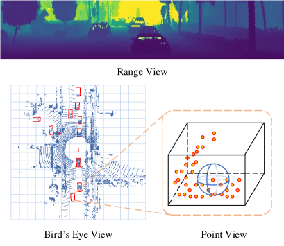
Figure 1: Different views in LiDAR-based 3D object detection.

LiDAR-based 3D object detection is an indispensable technology in the autonomous driving scenario. Though shared some similarities, object detection in the 3D sparse point cloud is fundamentally different from its 2D counterpart. The key is to efficiently represent the sparse and unordered point clouds for subsequent processing. Several popular representations include Bird’s Eye View (BEV) [10, 38, 37], Point View (PV) [25], Range View (RV) [12, 18] and fusion of them [24, 44, 33], which are shown in Fig.1. Among them, BEV is the most popular one. However, it introduces quantization error when dividing the space into the voxels or pillars, which is unfriendly for the distant objects that may only have few points. To overcome this drawback, the point view representation is usually incorporated. Point view operators [22, 23, 34, 31, 35, 30, 17] can extract effective features from unordered point clouds, but they are difficult to scale up to large-scale point cloud data efficiently in autonomous driving scenes.

The range view is widely adopted in semantic segmentation task [19, 36, 42, 43], but it is rarely used in object detection task individually. However, in this paper, we argue that the range view itself is the most compact and informative way for representing the LiDAR point clouds because it is generated from a single viewpoint. It essentially forms a 2.5D [8] scene instead of a full 3D point cloud. Consequently, organizing the point cloud in range view misses no information. The compactness also enables fast neighborhood queries based on range image coordinates, while point view methods usually need a time-consuming ball query algorithm [23] to get the neighbors. Moreover, the valid detection range of range-view-based detectors can be as far as the sensor’s availability, while we have to set a threshold for the detection range in BEV-based 3D detectors. Despite its advantages, an intriguing question raised, Why are the results of range-view-based LiDAR detection inferior to other representation forms?

Indeed some works have made attempts to make use of the range view representation from the pioneering work VeloFCN [12] to LaserNet [18] to the recently proposed RCD [1]. However, there is still a huge gap between the pure range-view-based method and the BEV-based method. For example, on the validation split of Waymo Open Dataset (WOD) [29], they are still lower than state-of-the-art methods by a large margin (more than 20 points 3D AP in vehicle class).

To liberate the power of range view representation, we examine the designs of the current range-view-based detectors and found several overlooked facts. These points seem simple and obvious, but we find that the devils are in the details. Properly handling these challenges is the key to high-performance range-view-based detection.

First, the challenge of detecting objects with sparse points in BEV is converted to the challenge of scale variation in the range image. Though there have been many methods [14, 13] in 2D object detection tried to address this issue, this challenge is never seriously considered in the range-view-based 3D detector.

Second, unlike in 2D image, though the convolution on range image is conducted on 2D pixel coordinates, while the output is in the 3D space. This point suggests an inferior design in the current range-view-based detectors: both the kernel weight and aggregation strategy of standard convolution ignore this inconsistency, which leads to severe geometric information loss even from the very beginning of the network.

Third, the 2D range view is naturally more compact than 3D space, which makes feature extractions in range-image-based detectors more efficient. However, how to utilize such characteristics to improve the performance of detectors is ignored by current range-image-based designs.

In this paper, we propose a pure range-view-based framework – RangeDet, which is a single-stage anchor-free detector designated to address the aforementioned challenges. We analyze the defects of the existing range-view-based 3D detector and point out the aforementioned three key challenges that need to be addressed. For the first challenge, we propose a simple yet effective Range Conditioned Pyramid to mitigate it. For the second challenge, we propose Meta-Kernel to capture 3D geometric information from 2D range view representation. For the third one, we use weighted Non-Maximum Suppression to remedy the issue. In addition to these techniques, we also explore how to transfer common data augmentation techniques from 3D space to the range view. Combining all the techniques, our best model achieves comparable results with state-of-the-art works in multiple views. And we surpass previous pure range-view-based detectors by a margin of 20 3D AP in vehicle detection. Interestingly, in contrast to common belief, RangeDet is more advantageous for farther or small objects than BEV representation.

2 Related Work

BEV-based 3D detectors. Several approaches for LiDAR-based 3D detection discretize the whole 3D space. 3DFCN [11] and PIXOR [38] encode handcrafted features into voxels, while VoxelNet [45] is the first to use end-to-end learned voxel features. SECOND [37] accelerates VoxelNet by sparse convolution. PointPillars [10] is aggressive in feature reduction that it applies PointNet to collapse the height dimension first and then treat it as a pseudo-image.

Point-view-based 3D detectors. F-PointNet [21] first generates frustums corresponding to 2D Region of Interest (ROI), then use PointNet [22] to segment foreground points and regress the 3D bounding boxes. PointRCNN [25] generates 3D proposals directly from the whole point clouds instead of 2D images for 3D detection with point clouds by using PointNet++ [23] both in proposal generation and refinement. IPOD [39] and STD [40] are both two-stage methods which use the foreground point cloud as a seed to generate proposals and refine them in the second stage.

Range-view-based 3D detectors. VeloFCN [12] is a pioneering work in range image detection, which projects point cloud to 2D and applies 2D convolutions to predict 3D box for each foreground point densely. LaserNet [18] uses a fully convolutional network to predict a multimodal distribution for each point to generate the final prediction. Recently, RCD [1] addresses the challenges in range-view based detection by learning a dynamic dilation for scale variation and soft range gating for the “boundary blur” issue as pointed in Pseudo-LiDAR [32].

Multi-view-based 3D detectors. MV3D [2] is the first work to fuse features in frontal view, BEV, and camera view for 3D object detection. PV-RCNN [24] jointly encodes point and voxel information to generate high-quality 3D proposals. MVF [44] endows a wealth of contextual information from different perspectives for each point to improve the detection of small objects.

2D detectors. Scale variation is a long-standing problem in 2D object detection. SNIP [27] and SNIPER [28] rescale proposals to a normalized size explicitly based on the idea of image pyramids. FPN [14] and its variants [16, 20] build feature pyramids, which have become the indispensable component for modern detectors. TridentNet [13] constructs weight-shared branches but using different dilation to build scale-aware feature maps.

3 Review of Range View Representation

In this section, we quickly review the range view representation of LiDAR data.

For a LiDAR with $m$ beams and $n$ times measurement in one scan cycle, the returned values from one scan form a $m\times n$ matrix, called range image (Fig. 1). Each column of the range image shares an azimuth, and each row of the range image shares an inclination. They indicate the relative vertical and horizontal angle of a returned point w.r.t the LiDAR original point. The pixel value in the range image contains the range (depth) of the corresponding point, the magnitude of the returned laser pulse called intensity and other auxiliary information. One pixel in the range image contains at least three geometric values: range $r$, azimuth $\theta$, and inclination $\phi$. These three values then define a spherical coordinate system. Fig. 2 illustrates the formation of the range image and these geometric values.

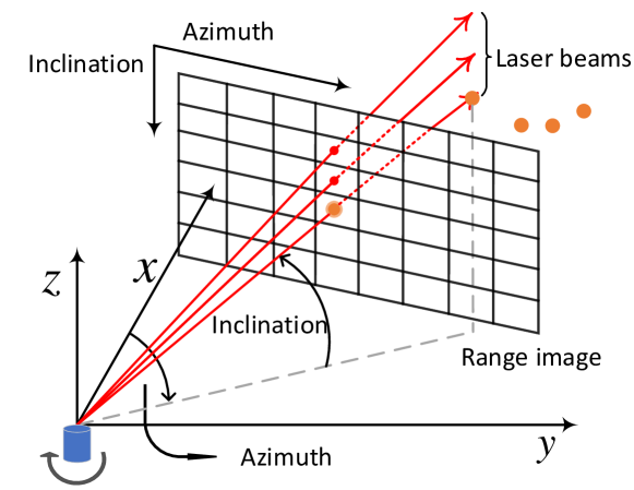
Figure 2: The illustration of the native range image.

The commonly-used point cloud data with Cartesian coordinates is actually decoded from the spherical coordinate system:

$$x =r\cos(\phi)\cos(\theta),$$ (1)

$$y =r\cos(\phi)\sin(\theta),$$

$$z =r\sin(\phi),$$

where $x,y,z$ denote the Cartesian coordinates of points. Note that range view is only valid for the scan from one viewpoint. It is not available for general point cloud since they may overlap for one pixel in the range image.

Unlike other LiDAR datasets, WOD directly provides the native range image. Except for range and intensity values, WOD also provides another information called elongation [29]. The elongation measures the extent to which the width of the laser pulse is elongated, which helps distinguish spurious objects.

4 Methodology

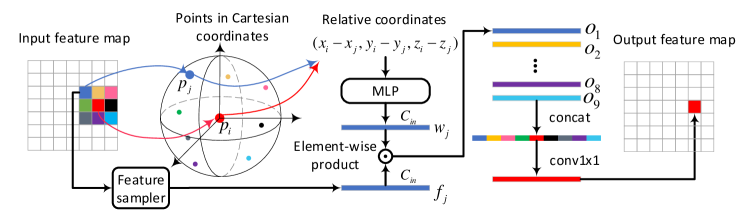
Figure 3: The illustration of Meta-Kernel (best viewed in color). Taking a 3x3 sampling grid as an example, we can get relative Cartesian coordinates of nine neighbors to the center. A shared MLP takes these relative coordinates as input to generate nine weight vectors: ${w_{1},w_{2},\cdots,w_{9}}$. Then we sample nine input feature vectors:${f_{1},f_{2},\cdots,f_{9}}$. $o_{i}$ is the element-wise product of $w_{i}$ and $f_{i}$. By passing a concatenation of $o_{i}$ from nine neighbors to a $1\times 1$ convolution, we aggregate the information from different channels and different sampling locations and get the output feature vector.

In this section, we first elaborate on three components of RangeDet. Then the full architecture is presented.

4.1 Range Conditioned Pyramid

In 2D detection, feature-pyramid-based methods such as Feature Pyramid Network (FPN) [14] are usually adopted to address the scale variation issue. We first construct the feature pyramids as in FPN which is illustrated in Fig. 4. Although the construction of the feature pyramid is similar to that of FPN in 2D object detection, the difference lies in how to assign each object to a different layer for training. In the original FPN, the ground-truth bounding box is assigned based on its area in the 2D image. Nevertheless, simply adopting this assignment method ignores the difference between the 2D range image and 3D Cartesian space. A nearby passenger car may have similar area with a far away truck but their scan patterns are largely different. Therefore, we designate the objects with a similar range to be processed by the same layer instead of purely using the area in FPN. Thus we name our structure as Range Conditioned Pyramid (RCP).

4.2 Meta-Kernel Convolution

Conv Type	Space	Sampling	Weight acquisition	Multiplication	Aggregation
Standard Conv	2D	Grid	Network parameter	Matrix multiplication	Channel-wise summation
Depth-wise Conv [3]	2D	Grid	Network parameter	Element-wise product	Channel-wise summation
RCD [1]	2D	Learned dilation	Network parameter	Matrix multiplication	Channel-wise summation
Deformable Conv [4]	2D	Learned offset	Network parameter	Matrix multiplication	Channel-wise summation
PointNet [22]	3D	Ball query	Network parameter	Matrix multiplication	Max-pooling
Continuous Conv [31]	3D	$k$NN	Generated by MLP	Matrix multiplication	Channel-wise summation
EdgeConv [34]	3D	$k$NN	Network parameter	Matrix multiplication	Max-pooling
RS Conv [17]	3D	Ball query	Generated by MLP	Element-wise product	Max-pooling
RandLA [9]	3D	$k$NN	Network parameter	Matrix multiplication	Attentive pooling
KPConv [30]	3D	Ball query	Weighted sum of parameter	Matrix multiplication	Channel-wise summation
Meta-Kernel	2D	Grid	Generated by MLP	Element-wise product	Concat and $1\times 1$ convolution

Table 1: Comparison of different convolutions.

Compared with the RGB image, the depth information endows range images with a Cartesian coordinate system, however standard convolution is designed for 2D images on regular pixel coordinates. For each pixel within the convolution kernel, the weights only depend on the relative pixel coordinates, which can not fully exploit the geometric information from the Cartesian coordinates. In this paper, we design a new operator which learns dynamic weights from relative Cartesian coordinates or more meta-data, making the convolution more suitable to the range image.

For better understanding, we first disassemble standard convolution into four components: sampling, weight acquisition, multiplication and aggregation.

1) Sampling. The sampling locations in standard convolution is a regular grid ${\mathcal{G}}$, which has $k_{h}\times k_{w}$ relative pixel coordinates. For example, a common $3\times 3$ sampling grid with dilation 1 is:

$$\mathcal{G}=\{(-1,-1),(-1,0),...,(1,0),(1,1)\}.\vspace{-0.1cm}$$ (2)

For each location ${\mathbf{p}}_{0}$ on the input feature map ${\mathbf{F}}$, we usually sample feature vectors of its neighbors ${\mathbf{F}}({\mathbf{p}}_{0}+{\mathbf{p}}_{n})$, ${\mathbf{p}}_{n}\in{\mathcal{G}}$ using im2col operation.

2) Weight acquisition. The weight matrix ${\mathbf{W}}({\mathbf{p}}_{n})\in\mathbb{R}^{C_{out}\times C_{in}}$ for each sampling location $({\mathbf{p}}_{0}+{\mathbf{p}}_{n})$ depends on ${\mathbf{p}}_{n}$, and fixed for a given feature map. This is also called the “weight sharing” mechanism for convolution.

3) Multiplication. We decompose the matrix multiplication of the standard convolution into two steps. The first step is pixel-wise matrix multiplication. For each sampling point $({\mathbf{p}}_{0}+{\mathbf{p}}_{n})$, its output is defined as

$${\mathbf{o}}_{{\mathbf{p}}_{0}}({\mathbf{p}}_{n})=\mathbf{W(p}_{n})\cdot{\mathbf{F}}({\mathbf{p}}_{0}+{\mathbf{p}}_{n}).\vspace{-0.0cm}$$ (3)

4) Aggregation. After multiplication, the second step is to sum over all the ${\mathbf{o}}_{{\mathbf{p}}_{0}}({\mathbf{p}}_{n})$ in ${\mathcal{G}}$, which is called channel-wise summation.

In summary, the standard convolution can be presented as:

$${\mathbf{z}}({\mathbf{p}}_{0})=\sum_{{\mathbf{p}}_{n}\in{\mathcal{G}}}{\mathbf{o}}_{{\mathbf{p}}_{0}}({\mathbf{p}}_{n}).$$ (4)

In our range view convolution, we expect that the convolution operation is aware of the local 3D structure. Thus, we make the weight adaptive to the local 3D structure via a meta-learning approach.

For weight acquisition, we first collect the meta-information of each sampling location and denote this relationship vector as ${\mathbf{h}}({\mathbf{p}}_{0},{\mathbf{p}}_{n})$. ${\mathbf{h}}({\mathbf{p}}_{0},{\mathbf{p}}_{n})$ usually contains relative Cartesian coordinates, range value, etc. Then we generate the convolution weight ${\mathbf{W}}_{{\mathbf{p}}_{0}}({\mathbf{p}}_{n})$ based on ${\mathbf{h}}({\mathbf{p}}_{0},{\mathbf{p}}_{n})$. Specifically, We apply a Multi-Layer Perceptron (MLP) with two fully-connected layers:

$${\mathbf{W}}_{{\mathbf{p}}_{0}}({\mathbf{p}}_{n})=\texttt{MLP}({\mathbf{h}}({\mathbf{p}}_{0},{\mathbf{p}}_{n})).$$ (5)

For multiplication, instead of matrix multiplication, we simply use element-wise product to obtain ${\mathbf{o}}_{{\mathbf{p}}_{0}}({\mathbf{p}}_{n})$ as follows:

$${\mathbf{o}}_{{\mathbf{p}}_{0}}({\mathbf{p}}_{n})={\mathbf{W}}_{{\mathbf{p}}_{0}}({\mathbf{p}}_{n})\odot{\mathbf{F}}({\mathbf{p}}_{0}+{\mathbf{p}}_{n}).$$ (6)

We do not use matrix multiplication because our algorithm runs on large-scale point clouds, and it costs too much GPU memory to save a weight tensor with shape $H\times W\times C_{out}\times k_{h}\times k_{w}\times C_{in}$. Inspired by the depth-wise convolution, the element-wise product eliminates the $C_{out}$ dimension from the weight tensor, which is much less memory-consuming. However, there is no cross-channel fusion in the element-wise product. We leave it to the aggregation step.

For aggregation, instead of channel-wise summation, we concatenate all ${\mathbf{o}}_{{\mathbf{p}}_{0}}({\mathbf{p}}_{n})$, $\forall{\mathbf{p}}_{n}\in{\mathcal{G}}$ and pass it to a fully-connected layer to aggregate the information from different channels and different sampling locations.

Summing it up, the Meta-Kernel can be formulated as:

$${\mathbf{z}}({\mathbf{p}}_{0})=\mathcal{A}({\mathbf{W}}_{{\mathbf{p}}_{0}}({\mathbf{p}}_{n})\odot{\mathbf{F}}({\mathbf{p}}_{0}+{\mathbf{p}}_{n})),\quad\forall{\mathbf{p}}_{n}\in{\mathcal{G}},$$ (7)

where $\mathcal{A}$ is the aggregation operation containing concatenation and a fully-connected layer. Fig. 3 provides a clear illustration of Meta-Kernel.

Comparison with point-based operators. Although shares some similarities with point-based convolution-like operators, Meta-Kernel has three significant differences from them. (1) Definition space. Meta-Kernel is defined in 2D range view, while others are defined in the 3D space. So Meta-Kernel has regular $n\times n$ neighborhood, and point-based operators have an irregular neighborhood. (2) Aggregation. Points in 3D space are unordered, so the aggregation step in point-based operators is usually permutation-invariant. Max-pooling and summation are widely adopted. $n\times n$ neighbors in the RV are permutation-variant, which is a natural advantage for Meta-Kernel to adopt concatenation and fully-connected layer as the aggregation step. (3) Efficiency. Point-based operators involve time-consuming key-point sampling and neighbor query. For example, downsampling 160K points to 16K with Farthest Point Sampling (FPS) [23] takes 6.5 seconds in a single 2080Ti GPU, which is also analyzed in RandLA-Net [9]. Some point-based operators, such as PointConv [35], KPConv [30] and the native version of Continuous Conv [31], generate a weight matrix or feature matrix for each point, so they face severe memory issue processing large-scale point cloud. These disadvantages make it impossible to apply point-based operators to large-scale point clouds (more than $10^{5}$ points) in autonomous driving scenarios.

For a clear comparison, we summarize the differences between several closely related work and our Meta-Kernel convolution in Table 1.

4.3 Weighted Non-Maximum Suppression

As mentioned earlier, how to utilize the compactness of range view representation to improve the performance of range-image-based detectors is an important topic. In common object detectors, a proposal inevitably has a random deviation from the mean of the proposal distribution. The straightforward way to get a proposal with small deviation is to choose the one with the highest confidence. While a better and more robust way to eliminate the deviation is using the majority votes of all the available proposals. An off-the-shelf technique just fits our need – weighted NMS [6]. Here comes an advantage of our method: the nature of compactness makes RangeDet feasible to generate proposals in the full-resolution feature map without huge computation cost, however it is infeasible for most BEV-based or point-view-based methods. With more proposals, the deviation will be better eliminated.

We first filter out the proposals whose scores are less than a predefined threshold 0.5, and then sort the proposals as in standard NMS by their predicted scores. For the current top-rank proposal $\mathbf{b_{0}}$, we find the proposals whose IoUs with $\mathbf{b_{0}}$ are higher than 0.5. The output bounding box for $\mathbf{b_{0}}$ is a weighted average of these proposals, which can be described as:

$$\mathbf{\widehat{b}_{0}}=\frac{\sum_{k}\mathbb{I}(\text{IoU}(\mathbf{b_{0}},\mathbf{b_{k}})>t)s_{k}\mathbf{b_{k}}}{\sum_{k}\mathbb{I}(\text{IoU}(\mathbf{b_{0}},\mathbf{b_{k}})>t)s_{k}},\vspace{-0.2cm}$$ (8)

where $\mathbf{b_{k}}$ and $s_{k}$ denote other proposals and corresponding scores. $t$ is the IoU threshold, which is 0.5. $\mathbb{I}(\cdot)$ is the indicator function.

4.4 Data Augmentation in Range View

Data augmentation is a critical technique to improve the performance of LiDAR-based 3D object detectors. Random global rotation, Random global flip and Copy-Paste are three typical ones. Although they are straightforward in 3D space, it’s non-trivial to transfer them to RV and preserve the structure of RV.

Rotation of point clouds can be regarded as translation of range images along the azimuth direction. Flipping in 3D space corresponds to the flipping with respect to one or two vertical axes of range images (We provide a clear illustration in supplementary materials). From the leftmost column to the rightmost, the span of azimuth is $(-\pi,\pi)$. So, unlike the augmentation of 2D RGB-image, we calculate the new coordinate of each point to keep it consistent with its azimuth. For Copy-Paste [37], the objects are pasted on the new range image with their original vertical pixel coordinates. Because of the non-uniform vertical angular resolution, we can only keep the structure of RV and avoid objects largely deviating from the ground by this treatment. Besides, a car in the distance should not be pasted in the front of a nearby wall. So we carry out “range test” to avoid such a situation.

4.5 Architecture

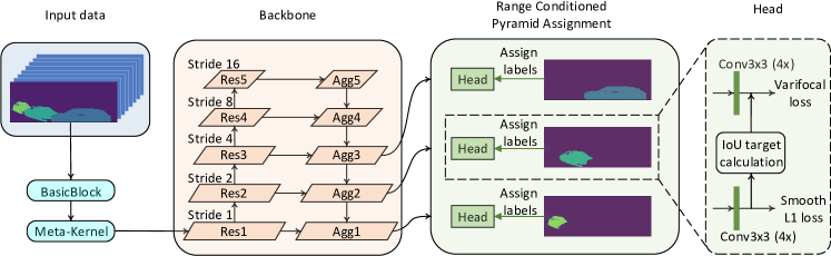
Figure 4: The overall architecture of RangeDet.

Overall pipeline. The architecture of RangeDet is shown in Fig. 4. The eight input range image channels include range, intensity, elongation, x, y, z, azimuth, and inclination, as described in Sec. 3. Meta-Kernel is placed in the second BasicBlock[7]. Feature maps are downsampled to stride 16, and upsampled to full resolution gradually. Next, we assign each ground-truth bounding box to the layers of stride $1,2,4$ in RCP according to the range of the box center. All the positions whose corresponding points are in ground-truth 3D bounding boxes are treated as positive samples, otherwise negative. At last, we adopt Weighted NMS to de-duplicate the proposals and generate high-quality results.

RCP and Meta-Kernel. In WOD, the range of a point varies from 0m to 80m. According to the distribution of points in the ground-truth bounding boxes, we divide $[0,80]$ to 3 intervals: $[0,15),[15,30),[30,80]$. We a use two-layer MLP with 64 filters to generate weights from relative Cartesian coordinates. ReLU is adopted as activation.

IoU Prediction head. In the classification branch, we adopt a very recent work – varifocal loss[41] to predict IoU between the predicted bounding box and the ground-truth bounding box. Our classification loss is defined as:

$$L_{\mathrm{cls}}=\frac{1}{M}\sum_{i}{\text{VFL}_{i}},\vspace{-0.2cm}$$ (9)

where $M$ is the number of valid points, and $i$ is the point index. $\text{VFL}_{i}$ is the varifocal loss of each point:

$$\begin{split}\text{VFL}(p,q)=\left\{\begin{array}[]{ll}-q(q\log(p)+(1-q)\log(1-p)),q>0\\ -\alpha p^{\gamma}\log(1-p),\qquad\qquad\qquad\quad q=0,\end{array}\right.\end{split}\vspace{-0.2cm}$$ (10)

where $p$ is the predicted score, and $q$ is the IoU between the predicted bounding box and the ground-truth bounding box. $\alpha$ and $\gamma$ play a similar role as in focal loss [15].

Regression head. The regression branch also contains four $3\times 3$ Conv as in the classification branch. We first formulate the ground-truth bounding box containing point $i$ as $(x_{i}^{g},y_{i}^{g},z_{i}^{g},l_{i}^{g},w_{i}^{g},h_{i}^{g},\theta_{i}^{g})$ to denote the coordinates of the bounding box center, dimension and orientation, respectively. The Cartesian coordinate of point $i$ is $(x_{i},y_{i},z_{i})$. We define the offsets between the point $i$ and the center of bounding box containing point $i$ as $\Delta r_{i}=r_{i}^{g}-r_{i},\;r\in\{x,y,z\}$. For point $i$, we regard its azimuth direction as its local $x$-axis which is the same as in LaserNet [18]. And we formulate such transformation as follows (Fig. 5 provides a clear illustration):

$$\alpha_{i} =\text{arctan2}\left(y_{i},x_{i}\right),$$ (11)

$$\boldsymbol{R_{i}} =\left[\begin{array}[]{ccc}\cos\alpha_{i}&\sin\alpha_{i}&0\\ -\sin\alpha_{i}&\cos\alpha_{i}&0\\ 0&0&1\\ \end{array}\right],$$

$$\phi_{i}^{g}=\theta_{i}^{g}-\alpha_{i}, \left[\Omega x_{i},\Omega y_{i},\Omega z_{i}\right]=\boldsymbol{R_{i}}\left[\Delta x_{i},\Delta y_{i},\Delta z_{i}\right]^{\top},$$

where $\alpha_{i}$ denotes the azimuth of point $i$, and $\left[\Omega x_{i},\Omega y_{i},\Omega z_{i}\right]$ is the transformed coordinate offset to be regressed. Such a transformed target is appropriate for range-image-based detection since an object’s appearance in the range image doesn’t change with the azimuth in a fixed range. Thus, it’s reasonable to make regression targets azimuth-invariant. So for each point, we regard azimuth direction as local $x$-axis.

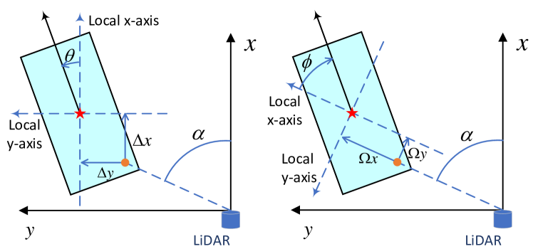
Figure 5: The illustration of two kinds of regression targets. Left: For all the points, the $x$-axis of the egocentric coordinate system is regarded as the local $x$-axis. Right: For each point, its azimuth direction is regarded as local $x$-axis. Before calculating the regression loss, we first transform the first kind of targets to the latter.

We denote the point $i$’s ground-truth targets set $\mathcal{Q}_{i}$ as $\left\{\Omega x_{i}^{g},\Omega y_{i}^{g},\Omega z_{i}^{g},\log l_{i}^{g},\log w_{i}^{g},\log h_{i}^{g},\cos\phi_{i}^{g},\sin\phi_{i}^{g}\right\}$. So the regression loss is defined as

$$L_{\mathrm{reg}}=\frac{1}{N}\sum_{i}\left(\frac{1}{n_{i}}\sum_{q_{i}\in\mathcal{Q}_{i}}\mathrm{SmoothL1}(q_{i}-p_{i})\right),\vspace{-0.2cm}$$ (12)

where $p_{i}$ is the predicted counterpart of $q_{i}$. $N$ is the number of ground-truth bounding boxes, and $n_{i}$ is the number of points in the bounding box which contains the point $i$. The total loss is the sum of $L_{cls}$ and $L_{reg}$.

5 Experiments

We conduct our experiments on large-scale Waymo Open Dataset (WOD), which is the only dataset that provides native range images. We report LEVEL_1 average precision in all experiments for comparing with other methods. Please refer to supplemental material for the detailed results and configuration of the pipeline. Experiments in Table 2, Table 4 and Table 10 using the entire training dataset. And we uniformly sample 25% training data ($\sim 40$k frames) for other experiments.

	Meta- Kernel	RCP	IoU Prediction	WNMS	DA	3D AP (IoU=0.7)				BEV AP (IoU=0.7)
						Overall	0 - 30	30 - 50	50 - inf	Overall	0 - 30	30 - 50	50 - inf
A1						53.39	73.02	48.79	28.14	70.45	86.22	68.45	51.90
A2	✓					56.58	76.11	54.29	32.53	74.89	88.14	71.43	57.55
A3		✓				58.37	78.66	50.40	32.35	78.02	90.71	73.13	62.23
A4	✓	✓				61.05	80.11	54.59	35.95	80.65	92.12	78.20	66.58
A5	✓	✓	✓			64.61	84.87	61.13	40.87	82.32	93.17	80.49	68.98
A6	✓	✓	✓	✓		69.00	86.89	66.16	45.81	85.48	93.62	82.17	72.97
A7	✓		✓	✓		64.35	82.60	60.11	39.91	77.33	89.19	75.69	61.33
A8			✓	✓		61.08	81.78	58.07	36.22	76.20	88.78	72.31	58.94
A9	✓	✓	✓	✓	✓	72.85	87.96	69.03	48.88	86.94	94.35	85.66	77.01

Table 2: Ablation of our components on vehicle detection. DA stands for data augmentation.

5.1 Study of Meta-Kernel Convolution

We conduct extensive experiments to ablate Meta-Kernel in this section. These experiments do not involve data augmentation. We build our baseline by replacing Meta-Kernel with a 2D $3\times 3$ convolution.

Different input features. Table 3 shows the results of different meta information as input. Not surprisingly, using relative pixel coordinates (E4) only brings marginal improvements compared with the baseline, demonstrating the necessity of Cartesian information (coordinates or range) in kernel weight.

	Meta-data	3D AP
E1	Baseline	63.57
E2	$(x_{i}-x_{j},y_{i}-y_{j},z_{i}-z_{j})$	67.00
E3	$(x_{j},y_{j},z_{j})$	64.05
E4	$(u_{i}-u_{j},v_{i}-v_{j})$	63.87
E5	$(x_{i},y_{i},z_{i},x_{j},y_{j},z_{j})$	65.33
E6	$(r_{i}-r_{j})$	67.31
E7	$(x_{i}-x_{j},y_{i}-y_{j},z_{i}-z_{j},r_{i}-r_{j})$	67.37
E8	$(x_{i}-x_{j},y_{i}-y_{j},z_{i}-z_{j},u_{i}-u_{j},v_{i}-v_{j})$	67.11

Table 3: Performance comparison of different inputs for our Meta-Kernel. In baseline experiment, Meta-Kernel is replaced by a $3\times 3$ 2D convolution. $(x_{i},y_{i},z_{i})$, $(u_{i},v_{i})$ and $r_{i}$ stand for Cartesian coordinates, pixel coordinates and range, respectively.

Method	View	3D AP on Vehicle (IoU=0.7)				3D AP on Pedestrian (IoU=0.5)
		Overall	0m - 30m	30m - 50m	50m - inf	Overall	0m - 30m	30m - 50m	50m - inf
PointPillars$\ast$ [10]	BEV	56.62	81.01	51.75	27.94	59.25	67.99	57.01	41.29
PointPillars${\dagger}$ [10]	BEV	62.2	81.8	55.7	31.2	60.0	68.9	57.6	46.0
DynVox[44]	BEV	59.29	84.9	56.08	31.07	60.83	69.76	58.43	42.06
MVF [44]	BEV + RV	62.93	86.3	60.2	36.02	65.33	72.51	63.35	50.62
PillarOD [33]	BEV + CV	69.8	88.53	66.5	42.93	72.51	79.34	72.14	56.77
Voxel-RCNN [5]	BEV	75.59	92.49	74.09	53.15	-	-	-	-
PointPillars$\P$ [10]	BEV	71.56	-	-	-	70.61	-	-	-
PV-RCNN [24]	BEV + PV	70.3	91.92	69.21	42.17	-	-	-	-
LaserNet [18]	RV	52.11	70.94	52.91	29.62	63.4	73.47	61.55	42.69
RCD (the first stage) [1]	RV	55.01	-	-	-	-	-	-	-
RCD [1]	RV + PV	66.39	86.59	65.64	40.00	-	-	-	-
Ours	RV	72.85	87.96	69.03	48.88	75.94	82.20	75.39	65.74

Table 4: Results of vehicle and pedestrian evaluated on WOD validation split. Please refer to supplementary materials for detailed results of cyclist. BEV: Bird’s Eys View. RV: Range View. CV: Cylindrical View [33]. PV: Point View. ${\dagger}$: implemented by [29]. $\P$: implemented by MMDetection3D. $\ast$: implemented by [44]. The best result and the second result are marked in red and blue, respectively.

Different locations to place Meta-Kernel. We place the Meta-Kernel at stages with different strides. The results are shown in Table 5, which demonstrates that Meta-Kernel is more prominent at a lower level. This result is reasonable since the low-level layers have a closer association with geometric structure, where the Meta-Kernel takes a vital role.

Stage stride	Baseline	1	2	4	8
3D AP	63.57	67.37	64.79	63.66	63.80

Table 5: Performances on vehicle class when Meta-Kernel is placed in different stages of different strides.

Performance on small objects. Boundary information is more crucial for small objects in range view, for example pedestrian, to avoid being diluted by background than large objects. Meta-Kernel enhances the boundary information by capturing local geometric features, so it is especially powerful in small objects detection. Table 6 shows the significant effectiveness.

Method	3D AP on Pedestrian (IoU=0.5)
	Overall	0 - 30	30 - 50	50 - inf
w/o Meta-Kernel	69.06	77.86	67.79	53.94
w/ Meta-Kernel	74.16	80.86	73.54	63.21
Improvements	+5.09	+3.00	+5.75	+9.27

Table 6: Ablation of Meta-Kernel on pedestrian.

Comparison with point-based operators. We discussed the main differences between Meta-Kernel and point-based operators in Sec. 4.2. For a fair comparison, we implement some typical point-based operators on the 2D range image with fixed $3\times 3$ neighborhood just like our Meta-Kernel. Please refer to supplementary materials for the implementation details. Some operators such as KPConv [30], PointConv [35] are not implemented due to huge memory costs. These methods all obtain inferior results as Table 7 shows. We owe it to the strategies they used for aggregation in unordered point clouds, which will be elaborated next.

Method	3D AP on Vehicle (IoU=0.7)
	Overall	0 - 30	30 - 50	50 - inf
2D Convolution	63.57	84.64	59.54	38.58
PointNet-RV [22]	63.47	84.43	59.32	38.29
EdgeConv-RV [34]	64.74	85.06	61.25	41.44
ContinuousConv-RV [31]	63.52	84.47	59.63	38.40
RSConv-RV [17]	63.47	84.45	59.70	38.13
RandLA-RV [9]	64.11	84.95	60.17	39.06
Meta-Kernel	67.37	85.91	62.61	42.77

Table 7: Comparison with point-based operators. The suffix “RV” means that the method is based on a fixed $3\times 3$ neighborhood in RV instead of the dynamic neighborhood in 3D space. ContinuousConv in this table is the efficient version.

Different ways of aggregation. Instead of concatenation, we try max-pooling and summation in a channel-wise manner just like other point-based operators, and Table 8 shows the results. Performance significantly drops when using max-pooling or summation as they treat the features from different locations equally. These results demonstrate the importance of keeping and utilizing the relative orders in range view. Note that other views cannot adopt concatenation due to the disorder of point clouds.

$\mathcal{A}$	Baseline	Max-pooling	Sum	Concate
3D AP	63.57	63.47	63.52	67.37

Table 8: Results of different aggregation strategies.

5.2 Study of Range Conditioned Pyramid

Instead of conditioning on the range, we try three other strategies to assign bounding boxes: azimuth span, projected area and visible area. The azimuth span of a bounding box is proportional to its width in the range image. The projected area is the area of a box projected into the range image. The visible area is the area of visible object parts. Note that area is the standard assign criterion in 2D detection. For a fair comparison, we keep the number of ground-truth boxes in a certain stride consistent between these strategies. Results are shown in Table 9. We owe the inferior results to the pose change as well as occlusion, which makes the same object fall into different layers with different pose or occlusion conditions. Such a result demonstrates that it is not enough to only consider the scale variation in the range image, since some other physical features, such as intensity, density, change with the range.

Conditions	3D AP on Vehicle (IoU=0.7)
	Overall	0 - 30	30 - 50	50 - inf
w/o RCP	63.17	81.70	58.59	38.99
Range	67.37	85.91	62.61	42.77
Span of azimuth	64.04	80.63	62.28	42.34
Projected area	63.97	83.50	60.87	41.71
Visible area	59.43	79.69	57.69	34.67

Table 9: Comparison of different assignment strategies.

5.3 Study of Weighted Non-Maximum Suppression

To support our claims in Sec. 8, we apply weighted NMS in two typical voxel-based methods – PointPillars [10] and SECOND [37] based on the strong baselines in MMDetection3D. Compared with RangeDet, the others generate fewer proposals due to memory and computational limits, which degrades the performance of weighted NMS as Table 10 shows.

5.4 Ablation Experiments

We further conduct ablation experiments on the components we use. Table 2 summarizes the results. Meta-Kernel is effective and robust in different settings. Both RCP and Weighted NMS significantly improve the performance of our whole system. Although IoU prediction is a common practice of recent 3D detectors [24, 26], it has a considerable effect on RangeDet, so we ablate it in Table 2.

Method	3D AP on Vehicle (IoU=0.7)
	RangeDet	PointPillars [10]	SECOND [37]
NMS	69.17	68.49	67.14
Weigted NMS	72.85	69.53	67.73
Improvements	+3.68	+1.04	+0.59

Table 10: Results of weighted NMS on different detectors.

5.5 Comparison with State-of-the-Art Methods

Table 4 shows that RangeDet outperforms other pure range-view-based methods, and is slightly behind the state-of-the-art BEV-based two-stage method. Among all the results, we observe an interesting phenomenon: In contrast to the stereotype that range view is inferior in long-range detection, RangeDet outperforms most other compared methods in the long-range metric (i.e. 50m - inf), especially in the pedestrian class. Unlike in the range view, the pedestrian is very tiny in BEV. This again verifies the superiority of the range view representation and the effectiveness of our remedies to the inconsistency between range view input and 3D Cartesian output space.

5.6 Runtime Evaluation

On Waymo Open Dataset, our model achieves 12 FPS evaluated on a single 2080Ti GPU without deliberate optimization. Note that our method’s runtime speed is not affected by the expansion of the valid detection distance, while the speed of BEV-based methods will quickly slow down as the maximum detection distance expands.

6 Conclusion

We present RangeDet, a range-view-based detection framework consisting of Meta-Kernel, Range Conditioned Pyramid, and weighted NMS. With our special designs, RangeDet utilizes the nature of range view to overcome a couple of challenges. RangeDet achieves comparable performance with state-of-the-art multi-view-based detectors.

References

- [1] Alex Bewley, Pei Sun, Thomas Mensink, Dragomir Anguelov, and Cristian Sminchisescu. Range Conditioned Dilated Convolutions for Scale Invariant 3D Object Detection. arXiv preprint arXiv:2005.09927, 2020.
- [2] Xiaozhi Chen, Huimin Ma, Ji Wan, Bo Li, and Tian Xia. Multi-View 3D Object Detection Network for Autonomous Driving. In CVPR, pages 1907–1915, 2017.
- [3] François Chollet. Xception: Deep Learning with Depthwise Separable Convolutions. In CVPR, pages 1251–1258, 2017.
- [4] Jifeng Dai, Haozhi Qi, Yuwen Xiong, Yi Li, Guodong Zhang, Han Hu, and Yichen Wei. Deformable Convolutional Networks. In ICCV, pages 764–773, 2017.
- [5] Jiajun Deng, Shaoshuai Shi, Peiwei Li, Wengang Zhou, Yanyong Zhang, and Houqiang Li. Voxel R-CNN: Towards High Performance Voxel-based 3D Object Detection. 2021.
- [6] Spyros Gidaris and Nikos Komodakis. Object detection via a multi-region semantic segmentation-aware CNN model. In ICCV, pages 1134–1142, 2015.
- [7] Kaiming He, Xiangyu Zhang, Shaoqing Ren, and Jian Sun. Deep Residual Learning for Image Recognition. In CVPR, pages 770–778, 2016.
- [8] Peiyun Hu, Jason Ziglar, David Held, and Deva Ramanan. What you see is what you get: Exploiting visibility for 3d object detection. In CVPR, pages 11001–11009, 2020.
- [9] Qingyong Hu, Bo Yang, Linhai Xie, Stefano Rosa, Yulan Guo, Zhihua Wang, Niki Trigoni, and Andrew Markham. RandLA-Net: Efficient semantic segmentation of large-scale point clouds. In CVPR, pages 11108–11117, 2020.
- [10] Alex H Lang, Sourabh Vora, Holger Caesar, Lubing Zhou, Jiong Yang, and Oscar Beijbom. PointPillars: Fast Encoders for Object Detection from Point Clouds. In CVPR, pages 12697–12705, 2019.
- [11] Bo Li. 3D Fully Convolutional Network for Vehicle Detection in Point Cloud. In IROS, pages 1513–1518, 2017.
- [12] Bo Li, Tianlei Zhang, and Tian Xia. Vehicle Detection from 3D Lidar Using Fully Convolutional Network. 2016.
- [13] Yanghao Li, Yuntao Chen, Naiyan Wang, and Zhaoxiang Zhang. Scale-Aware Trident Networks for Object Detection. In ICCV, pages 6054–6063, 2019.
- [14] Tsung-Yi Lin, Piotr Dollár, Ross Girshick, Kaiming He, Bharath Hariharan, and Serge Belongie. Feature Pyramid Networks for Object Detection. In CVPR, pages 2117–2125, 2017.
- [15] Tsung-Yi Lin, Priya Goyal, Ross Girshick, Kaiming He, and Piotr Dollár. Focal Loss for Dense Object Detection. In ICCV, pages 2980–2988, 2017.
- [16] Shu Liu, Lu Qi, Haifang Qin, Jianping Shi, and Jiaya Jia. Path Aggregation Network for Instance Segmentation. In CVPR, pages 8759–8768, 2018.
- [17] Yongcheng Liu, Bin Fan, Shiming Xiang, and Chunhong Pan. Relation-Shape Convolutional Neural Network for Point Cloud Analysis. In CVPR, pages 8895–8904, 2019.
- [18] Gregory P Meyer, Ankit Laddha, Eric Kee, Carlos Vallespi-Gonzalez, and Carl K Wellington. LaserNet: An Efficient Probabilistic 3D Object Detector for Autonomous Driving. In CVPR, pages 12677–12686, 2019.
- [19] Andres Milioto, Ignacio Vizzo, Jens Behley, and Cyrill Stachniss. RangeNet++: Fast and Accurate LiDAR Semantic Segmentation. In IROS, pages 4213–4220, 2019.
- [20] Jiangmiao Pang, Kai Chen, Jianping Shi, Huajun Feng, Wanli Ouyang, and Dahua Lin. Libra R-CNN: Towards Balanced Learning for Object Detection. In CVPR, pages 821–830, 2019.
- [21] Charles R Qi, Wei Liu, Chenxia Wu, Hao Su, and Leonidas J Guibas. Frustum PointNets for 3D Object Detection from RGB-D Data. In CVPR, pages 918–927, 2018.
- [22] Charles R Qi, Hao Su, Kaichun Mo, and Leonidas J Guibas. PointNet: Deep Learning on Point Sets for 3D Classification and Segmentation. In CVPR, pages 652–660, 2017.
- [23] Charles Ruizhongtai Qi, Li Yi, Hao Su, and Leonidas J Guibas. PointNet++: Deep Hierarchical Feature Learning on Point Sets in a Metric Space. In NeurIPS, pages 5099–5108, 2017.
- [24] Shaoshuai Shi, Chaoxu Guo, Li Jiang, Zhe Wang, Jianping Shi, Xiaogang Wang, and Hongsheng Li. PV-RCNN: Point-Voxel Feature Set Abstraction for 3D Object Detection. In CVPR, pages 10529–10538, 2020.
- [25] Shaoshuai Shi, Xiaogang Wang, and Hongsheng Li. PointRCNN: 3D Object Proposal Generation and Detection from Point Cloud. In CVPR, pages 770–779, 2019.
- [26] Shaoshuai Shi, Zhe Wang, Jianping Shi, Xiaogang Wang, and Hongsheng Li. From Points to Parts: 3D Object Detection from Point Cloud with Part-aware and Part-aggregation Network. IEEE Transactions on Pattern Analysis and Machine Intelligence, 2020.
- [27] Bharat Singh and Larry S Davis. An Analysis of Scale Invariance in Object Detection - SNIP. In CVPR, pages 3578–3587, 2018.
- [28] Bharat Singh, Mahyar Najibi, and Larry S Davis. SNIPER: Efficient Multi-Scale Training. In NeurIPS, pages 9310–9320, 2018.
- [29] Pei Sun, Henrik Kretzschmar, Xerxes Dotiwalla, Aurelien Chouard, Vijaysai Patnaik, Paul Tsui, James Guo, Yin Zhou, Yuning Chai, Benjamin Caine, et al. Scalability in Perception for Autonomous Driving: Waymo Open Dataset. In CVPR, pages 2446–2454, 2020.
- [30] Hugues Thomas, Charles R Qi, Jean-Emmanuel Deschaud, Beatriz Marcotegui, François Goulette, and Leonidas J Guibas. KPConv: Flexible and deformable convolution for point clouds. In ICCV, pages 6411–6420, 2019.
- [31] Shenlong Wang, Simon Suo, Wei-Chiu Ma, Andrei Pokrovsky, and Raquel Urtasun. Deep parametric continuous convolutional neural networks. In CVPR, pages 2589–2597, 2018.
- [32] Yan Wang, Wei-Lun Chao, Divyansh Garg, Bharath Hariharan, Mark Campbell, and Kilian Q Weinberger. Pseudo-LiDAR from Visual Depth Estimation: Bridging the Gap in 3D Object Detection for Autonomous Driving. In CVPR, pages 8445–8453, 2019.
- [33] Yue Wang, Alireza Fathi, Abhijit Kundu, David Ross, Caroline Pantofaru, Tom Funkhouser, and Justin Solomon. Pillar-based Object Detection for Autonomous Driving. In ECCV, 2020.
- [34] Yue Wang, Yongbin Sun, Ziwei Liu, Sanjay E Sarma, Michael M Bronstein, and Justin M Solomon. Dynamic graph cnn for learning on point clouds. Acm Transactions On Graphics (tog), 38(5):1–12, 2019.
- [35] Wenxuan Wu, Zhongang Qi, and Li Fuxin. PointConv: Deep convolutional networks on 3d point clouds. In CVPR, pages 9621–9630, 2019.
- [36] Chenfeng Xu, Bichen Wu, Zining Wang, Wei Zhan, Peter Vajda, Kurt Keutzer, and Masayoshi Tomizuka. SqueezeSegV3: Spatially-Adaptive Convolution for Efficient Point-Cloud Segmentation. arXiv preprint arXiv:2004.01803, 2020.
- [37] Yan Yan, Yuxing Mao, and Bo Li. SECOND: Sparsely Embedded Convolutional Detection. Sensors, 18(10):3337, 2018.
- [38] Bin Yang, Wenjie Luo, and Raquel Urtasun. PIXOR: Real-time 3D Object Detection from Point Clouds. In CVPR, pages 7652–7660, 2018.
- [39] Zetong Yang, Yanan Sun, Shu Liu, Xiaoyong Shen, and Jiaya Jia. IPOD: Intensive Point-based Object Detector for Point Cloud. arXiv preprint arXiv:1812.05276, 2018.
- [40] Zetong Yang, Yanan Sun, Shu Liu, Xiaoyong Shen, and Jiaya Jia. STD: Sparse-to-Dense 3D Object Detector for Point Cloud. In ICCV, pages 1951–1960, 2019.
- [41] Haoyang Zhang, Ying Wang, Feras Dayoub, and Niko Sünderhauf. VarifocalNet: An IoU-aware Dense Object Detector. arXiv preprint arXiv:2008.13367, 2020.
- [42] Yang Zhang, Zixiang Zhou, Philip David, Xiangyu Yue, Zerong Xi, Boqing Gong, and Hassan Foroosh. PolarNet: An Improved Grid Representation for Online LiDAR Point Clouds Semantic Segmentation. In CVPR, pages 9601–9610, 2020.
- [43] Hui Zhou, Xinge Zhu, Xiao Song, Yuexin Ma, Zhe Wang, Hongsheng Li, and Dahua Lin. Cylinder3D: An Effective 3D Framework for Driving-scene LiDAR Semantic Segmentation. arXiv preprint arXiv:2008.01550, 2020.
- [44] Yin Zhou, Pei Sun, Yu Zhang, Dragomir Anguelov, Jiyang Gao, Tom Ouyang, James Guo, Jiquan Ngiam, and Vijay Vasudevan. End-to-End Multi-View Fusion for 3D Object Detection in LiDAR Point Clouds. In CoRL, pages 923–932, 2020.
- [45] Yin Zhou and Oncel Tuzel. VoxelNet: End-to-End Learning for Point Cloud Based 3D Object Detection. In CVPR, pages 4490–4499, 2018.