1 Introduction

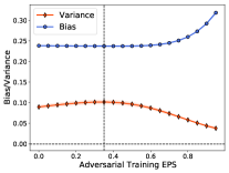
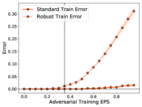
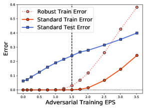
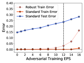
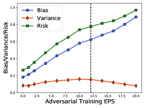
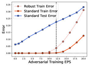
Adversarial training enhances the robustness of modern machine learning methods at the cost of decreased accuracy on the clean test samples (Goodfellow et al., 2014; Madry et al., 2017; Sinha et al., 2017). Though the model can fit the training data perfectly in adversarial training, the generalization error on clean test data increases compared with non-adversarially trained models. As illustrated in the right panel of Figure 1, adversarially trained models on CIFAR10 can achieve nearly zero robust training error, yet their test error still grows large as the perturbation radius $\varepsilon$ increases, even for clean test examples. To improve the robustness and accuracy of adversarially trained models, we thus seek to understand the cause for this increased “generalization gap” between errors on the training and test datasets.

To better understand this generalization gap, we turn to a standard tool of statistical learning theory, the bias-variance decomposition (Markov, 1900; Lehmann, 1983; Casella and Berger, 2001; Hastie et al., 2009; Geman et al., 1992). A large bias means the model predicts poorly on average, while a large variance means the predictions are very spread out. Adversarial training can be thought of as a form of regularization, and so we might expect it to increase bias and decrease variance. On the other hand, adversarial training intuitively makes the decision boundary more jagged and complex (Yang et al., 2020a), suggesting increased variance is the main cause. To arbitrate these different perspectives, we empirically investigate bias and variance across a variety of datasets as a function of the adversarial training radius $\varepsilon$.

Figure 1: Measuring the performance for $\ell_{\infty}$-adversarial training (with increasing perturbation size) on the CIFAR10 dataset. Standard error means the error rate on clean samples, and robust error means the error rate on adversarially perturbed samples. The vertical dashed line corresponds to the robust training error of the adversarially trained model reaching $2\%$ (i.e., robust interpolation threshold). (Left) Evaluating the bias, variance, and risk for the $\ell_{\infty}$-adversarially trained model (WideResNet-28-10). (Right) Evaluating robust training error, and standard training/test error on the same model.

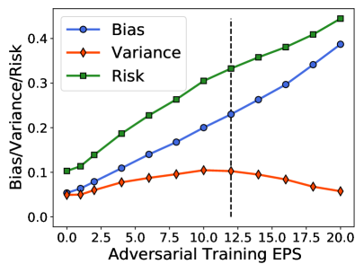
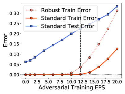
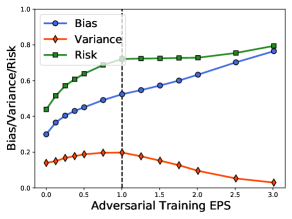
Interestingly, we find that both perspectives are incomplete–the variance is neither increasing nor decreasing with $\varepsilon$. Instead, we robustly observe the following behavior across several datasets. First, the bias is monotonically increasing in $\varepsilon$ and is the dominant term of the risk. Second, the variance is unimodal in $\varepsilon$: The variance increases up to some peak and then decreases. Moreover, the peak consistently occurs near the robust interpolation threshold–the minimum $\varepsilon$ for which the model can no longer robustly interpolate the training set.

The unimodal variance observation is surprising given that it contradicts both of the perspectives above, and its co-occurence with the interpolation threshold suggests a deeper phenomenon. We believe these observations are an inversion of the “double descent” phenomenon where larger models sometimes generalize better (Belkin et al., 2019; Nakkiran et al., 2020), and in particular echo observations in Yang et al. (2020), which finds the variance of a (regularly-trained) neural network to be unimodal as a function of width, with the peak also occurring at the interpolation threshold. We discuss this in more detail in Section 6.

Beyond their intrinsic interest, we draw two additional implications from the observed characteristic properties of bias and variance. First, since they can be robustly observed across many adversarial learning tasks, they can be used as criteria to check the validity of simplified conceptual models of adversarial training. If a simplified model fails to predict the correct behavior of bias and variance, then it has limitations for understanding adversarial training. We apply this test to several such models and find the following:

• The non-linearity of the predictor is not generally important: the monotonic bias and unimodal variance properties already (approximately) hold for logistic regression.

• The adaptivity of the attack is not important: the properties hold for randomized smoothing, which adds independent Gaussian noise to each minibatch.

• The dynamic nature of the attack is important: if we add fixed Gaussian noise to each minibatch (rather than new noise at each epoch) the properties cease to hold.

• The high dimensionality of the data is important: the properties fail to hold on certain key low-dimensional models, while being observable in the same models in high dimensions.

This last point in particular casts doubt on popular intuitions regarding the generalization gap in adversarial training, which are based on the ”jaggedness” of the decision boundary in low dimensions (Section 4.1). The observations above also shed light into the mechanism underlying the adversarial generalization gap: it is primarily a property of dynamic training noise in high-dimensional settings.

As a second implication, since the variance is dominated by the bias and decreases for large $\varepsilon$, scalable solutions to adversarial robustness must primarily address the bias. We therefore investigate several algorithms for improving adversarial robustness, to determine which ones decrease the bias. The common approach of early stopping (Rice et al., 2020) decreases variance, but slightly increases bias, so we cannot solely rely on it. Increasing the width also reduces variance, but not bias. However, we find that adding unlabeled data (Carmon et al., 2019; Uesato et al., 2019; Najafi et al., 2019; Zhai et al., 2019) and using pre-trained models (Hendrycks et al., 2019a) both decrease the bias, suggesting these may lead to scalable opportunities to achieve further robustness.

1.1 Related work

Robustness-accuracy tradeoff.

There is a large literature on understanding the trade-off between adversarial robustness and standard accuracy for adversarially robust classification problems. Classical works study robustness of linear models, showing equivalences between adversarially robust regression and lasso (Xu et al., 2009a, b). Recent works identify the fundamental robustness-accuracy trade-off in simplified theoretical models, where samples from different classes are close and there is no robust and accurate classifier (Fawzi et al., 2018; Zhang et al., 2019; Dobriban et al., 2020). Nakkiran (2019) argue theoretically that the tradeoff is due to the simplicity of the classifiers, suggesting that more complex classifiers are required for adversarial robustness. Tsipras et al. (2018) and Ilyas et al. (2019) argue that adversarially robust models are less accurate because they cannot rely on predictive, yet non-robust, features of the data. Other works characterize the robust error and trade-offs for linear models (Dan et al., 2020; Javanmard et al., 2020; Javanmard and Soltanolkotabi, 2020; Dobriban et al., 2020; Megyeri et al., 2019). Raghunathan et al. (2020) argue that unlabeled data can be used to mitigate the trade-off and improve model robustness. Yang et al. (2020b) empirically study the trade-off via local Lipschitzness. Other works study robustness for non-parametric methods (Wang et al., 2018; Bhattacharjee and Chaudhuri, 2020; Yang et al., 2020a).

Adversarially robust generalization.

Schmidt et al. (2018) consider a Gaussian classification model and show that adversarial training requires more data for generalization. Several previous works study the generalization and sample complexity via Rademacher complexity and VC dimension (Cullina et al., 2018; Attias et al., 2019; Yin et al., 2019; Khim and Loh, 2018; Montasser et al., 2019). Bubeck et al. (2018, 2019) argue that learning robust classifiers may be computationally hard. Other works study statistical properties of adversarial logistic regression (Javanmard and Soltanolkotabi, 2020; Dan et al., 2020; Dobriban et al., 2020; Taheri et al., 2020). Several works use the concentration of measure to study adversarial examples in high dimensions (Gilmer et al., 2018; Shafahi et al., 2019; Mahloujifar et al., 2019). Similarly, some works develop connections to optimal transport (Dohmatob, 2019; Bhagoji et al., 2019; Pydi and Jog, 2020).

Adversarial defenses and attacks.

A large body of literature is devoted to improving adversarial robustness (Goodfellow et al., 2014; Kurakin et al., 2016; Madry et al., 2017; Hein and Andriushchenko, 2017; Wong and Kolter, 2017; Sinha et al., 2017; Cohen et al., 2019; Raghunathan et al., 2018; Zhang et al., 2019; Wu et al., 2020) and developing adversarial attacks (Carlini and Wagner, 2017; Papernot et al., 2017; Athalye et al., 2018; Kang et al., 2019; Aboutalebi et al., 2020; Croce and Hein, 2020). Incorporating unlabeled data has been shown to be an effective approach for improving model adversarial robustness (Carmon et al., 2019; Uesato et al., 2019; Najafi et al., 2019; Zhai et al., 2019). Shah et al. (2020) argue that the “Simplicity Bias” in deep neural networks could be an explanation for the existence of universal adversarial examples. Gowal et al. (2020) show that by tuning the model size, activation function, and model weight averaging, adversarial training can achieve state-of-the-art $\ell_{\infty}$/$\ell_{2}$ adversarial robustness on the CIFAR10 dataset. Croce et al. (2020) recently benchmark adversarial $\ell_{\infty}$/$\ell_{2}$ robustness based on AutoAttack (Croce and Hein, 2020).

2 Preliminary

We review the bias-variance decomposition that will be used in later sections. We mainly consider the decomposition of the squared $\ell_{2}$ loss; extensions to the cross-entropy loss can be found in Appendices B and C.

Standard training and adversarial training.

For standard supervised $k$-class classification, we are given $n$ i.i.d. training samples ${\mathcal{T}}=\{({\boldsymbol{x}}_{i},{\boldsymbol{y}}_{i})\}_{i=1}^{n}$, a parameterized class of prediction functions $f_{{\boldsymbol{\theta}}}(\cdot)$—where $f_{{\boldsymbol{\theta}}}(\cdot),{\boldsymbol{y}}_{i}\in\mathbb{R}^{k}$— and a loss function $\ell(\cdot,\cdot)$ . The goal of standard training is to find parameters $\widehat{{\boldsymbol{\theta}}}({\mathcal{T}})$ that approximately solve the following problem:

$$\min_{{\boldsymbol{\theta}}}\frac{1}{n}\sum_{i=1}^{n}\ell\left(f_{\boldsymbol{\theta}}({\boldsymbol{x}}_{i}),{\boldsymbol{y}}_{i}\right).$$ (1)

Certain models learned through Eq. (1) are vulnerable to adversarial perturbations, especially some deep neural nets (Szegedy et al., 2013; Biggio et al., 2013). Adversarial training (AT) enhances the robustness of the model by solving the following robust optimization problem, for a set of perturbations $\Delta$:

$$\min_{{\boldsymbol{\theta}}}\frac{1}{n}\sum_{i=1}^{n}\max_{{\boldsymbol{\delta}}_{i}\in\Delta}\ell\left(f_{\boldsymbol{\theta}}({\boldsymbol{x}}_{i}+{\boldsymbol{\delta}}_{i}),{\boldsymbol{y}}_{i}\right).$$ (2)

In practice, the inner maximization is approximately solved by projected gradient descent (PGD), and the outer minimization is approximately solved by stochastic gradient descent (SGD) (Madry et al., 2017). We follow this adversarial training procedure in this paper. A typical choice for the perturbation set is the $\ell_{p}$ norm ball $\Delta=\{{\boldsymbol{\delta}}:\|{\boldsymbol{\delta}}\|_{p}\leq\varepsilon\}$.

Bias-variance decomposition.

Given a test point $({\boldsymbol{x}},{\boldsymbol{y}})$, an accurately trained model satisfies ${\boldsymbol{y}}\approx f_{\widehat{{\boldsymbol{\theta}}}}({\boldsymbol{x}})$. Therefore, for a good model, the prediction $f_{\widehat{{\boldsymbol{\theta}}}}({\boldsymbol{x}})$ should not depend too much on the training set ${\mathcal{T}}$. This is quantified by the variance:

$$\textsf{Var}=\mathbb{E}_{\boldsymbol{x}}\text{Var}_{{\mathcal{T}}}\left[f_{\widehat{{\boldsymbol{\theta}}}({\mathcal{T}})}({\boldsymbol{x}})\right],$$ (3)

which captures the variation in the prediction under different initialization of the training set. The variance depends on the training algorithm $\smash{{\mathcal{T}}\to\widehat{\boldsymbol{\theta}}({\mathcal{T}})}$ (and thus implicitly also on the sample size) and the data distribution. A large variance implies that the trained model $f_{\widehat{{\boldsymbol{\theta}}}}$ is sensitive to a particular realization of the training dataset ${\mathcal{T}}$, which is unfavorable. The bias term is

$$\textsf{Bias}=\mathbb{E}_{\widehat{{\boldsymbol{\theta}}},{\boldsymbol{x}},{\boldsymbol{y}}}\left\|{\boldsymbol{y}}-f_{\hat{{\boldsymbol{\theta}}}_{n}({\mathcal{T}})}({\boldsymbol{x}})\right\|_{2}^{2}-\textsf{Var}=\mathbb{E}_{{\boldsymbol{x}},{\boldsymbol{y}}}\left\|{\boldsymbol{y}}-\mathbb{E}_{\widehat{{\boldsymbol{\theta}}}}f_{\hat{{\boldsymbol{\theta}}}_{n}({\mathcal{T}})}({\boldsymbol{x}})\right\|_{2}^{2},$$

which captures how good the model performs on average.

Estimation of bias and variance.

To estimate the bias and variance of the models, we first partition the training dataset $\mathcal{T}$ into two disjoint parts $\mathcal{T}=\mathcal{T}_{1}\cup\mathcal{T}_{2}$. Then we rely on the bias-variance decomposition for the mean squared error $\|{\boldsymbol{y}}-f_{\widehat{{\boldsymbol{\theta}}}}({\boldsymbol{x}})\|^{2}$ (see previous paragraphs), where ${\boldsymbol{y}}$ is the one-hot encoding label vector and $f_{\widehat{{\boldsymbol{\theta}}}}({\boldsymbol{x}})$ is the output of the softmax layer. More details for estimating the bias and the variance can be found in Appendix B.

3 Measuring Bias and Variance for Deep Neural Networks

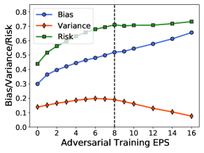
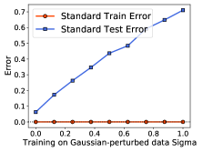
We study the bias-variance behavior of deep neural networks adversarially trained on the CIFAR10, CIFAR100, and ImageNet10 (a subset of 10 classes from ImageNet (Deng et al., 2009)) dataset. We find that the variance is unimodal and the bias is monotonically increasing (Figure 1 and 2) as a function of perturbation size. We find that the same phenomenon holds for randomized smoothing (another common robust training method), but not for training on noisy Gaussian-perturbed data (where the perturbations are fixed during training). Our code is available at https://github.com/yaodongyu/BiasVariance-AdversarialTraining.

3.1 Adversarially Trained Models

We first study the bias-variance decomposition for $\ell_{\infty}$ adversarially trained models with increasing perturbation size $\varepsilon$ on image classification tasks.

(a) CIFAR100.

(b) ImageNet10.

(c) CIFAR10 (early stopping).

Figure 2: Measuring bias-variance for $\ell_{\infty}$-adversarial training (with increasing perturbation size) on the CIFAR10 / CIFAR100 / ImageNet10 dataset. The vertical dashed line corresponds to the robust training error of the adversarially trained model being larger than $2\%$ (i.e., robust interpolation threshold). (a) CIFAR100 dataset. (b) ImageNet10 dataset. (c) CIFAR10 dataset (evaluated on early stopped models).

Experimental setup.

We train our models using stochastic gradient descent (SGD) with momentum 0.9, where the learning rate is 0.1, mini-batch size is 128, and the weight decay parameter is 0.0005. We train the models for 200 epochs and apply stage-wise learning rate decay during training, where we decay the learning rate by a factor of 0.1 at epochs 100 and 150. We use the Wide-ResNet architecture (WRN-28-10) (Zagoruyko and Komodakis, 2016) on CIFAR10 (Krizhevsky and Hinton, 2009), PreActResNet18 (He et al., 2016b) on CIFAR100, and ResNet18 (He et al., 2016a) on ImageNet10.

We consider a perturbation size $\varepsilon/255$ with $\varepsilon$ varying from $0$ to $16$ on CIFAR100 and ImageNet10, and use larger $\varepsilon$ on CIFAR10 ($0\leq\varepsilon\leq 20$). For the inner maximization in adversarial training, we apply a 10-step PGD attack with perturbation step size $\eta=0.25\cdot(\varepsilon/255)$. In addition to models trained to full convergence, we also study models that are stopped early, at the 100-th epoch. Early stopping has been shown to improve adversarial robustness (Zhang et al., 2019; Rice et al., 2020; Gowal et al., 2020). More detailed descriptions of the experimental setup can be found in Appendix C.

Bias-variance behavior.

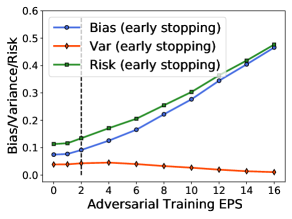
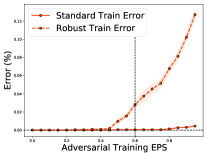
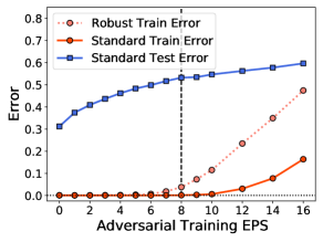
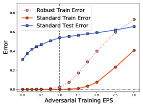
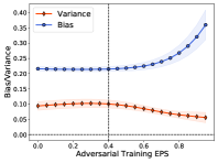
From Figure 1 (CIFAR10), Figure 2(a) (CIFAR100), and Figure 2(b) (ImageNet10), we observe several consistent properties of adversarial training:

1. The bias increases monotonically when we increase the perturbation size $\varepsilon$.

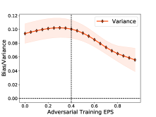
2. The variance first increases, then decreases, with $\varepsilon$.

3. The variance peak occurs near the point where the robust training error first starts to rise. We call this point the robust interpolation threshold and quantify it as the smallest $\varepsilon$ with larger than $2\%$ robust training error.

4. The bias is the dominant term in the risk.

Properties P1-P3 are reminiscent of previous findings related to double descent (Yang et al., 2020; Lin and Dobriban, 2020; Belkin et al., 2019; Nakkiran et al., 2020). There, the bias and variance exhibit similar behavior (for standard, non-robust training) when increasing another parameter, model width. Increasing $\varepsilon$ makes the data more complex and decreasing width make the model less powerful. Both make the learning task harder to interpolate and lead to a bias/varaince behavior that satisfy properties P1-P3. The connection here suggests a more general relation between the bias/variance behavior and the “hardness of interpolation”.

Table 1: Summary of bias-variance behavior of different training methods on various datasets. P1-P4 are 4 consistent properties of adversarial training (see Section 3.1 for detailed descriptions). (✓) – property is satisfied, (✗) – property is not satisfied, and (${\approx}$) – property is approximately satisfied.

TRAINING SETTING	DATASET	P1	P2	P3	P4	REFERENCE
Adversarial Training (AT)	Image	✓	✓	✓	✓	Section 3.1
Early Stopping-AT	Image	✓	✓	✓	✓	Section 3.1
Randomized Smoothing	Image	✓	✓	✓	✓	Section 3.2
(Fixed-)Gaussian Noise	Image	✓	✗	✗	✓	Section 3.2
Adversarial Training	Box Dataset ($d\leq 5$)	✓	✗	✗	✓	Section 4.1
Adversarial Training	Box Dataset ($d\geq 10$)	✓	✓	✓	✓	Section 4.1
Logistic Regression	Mixture of Gaussian	$\approx$	✓	✓	✓	Section 4.2
Logistic Regression	Planted Robust Feature	$\approx$	✓	✓	✓	Section 4.2

Early stopping.

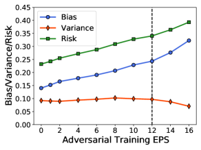
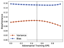
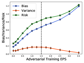
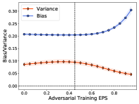
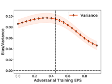
Figure 2(c) depicts the results of early stopping on CIFAR10. Compared with the fully trained model in Figure 1, the peak of the variance curve occurs earlier, but still coincides with the robust interpolation threshold. Indeed, each of properties P1-P4 still hold in this setting.

The early stopped model has lower risk than the fully trained model when $\varepsilon$ is small. However, the risk is lower due to decreased variance (the bias in fact increases slightly). Since the variance is already low (per P4), decreasing it further has limited effect. We therefore also need approaches for reducing the bias–we will study this further in Section 5.

Robustness checks.

Beyond the settings above, we observe properties P1-P4 for $\ell_{2}$-adversarial training and for a different bias-variance decomposition based on cross-entropy (Appendix C). We summarize the bias-variance behavior of various training methods in the first two rows of Table 1. In addition to standard adversarial training on the image classification tasks considered, we find that properties P1-P4 consistently hold in several other settings.

3.2 Training with Gaussian Noise

In this subsection, we study the bias-variance decomposition for two other training approaches: randomized smoothing and training on Gaussian-perturbed data. Randomized smoothing adds random Gaussian noise to each mini-batch used for the SGD updates, and has been used to obtain certifiably robust models (Lecuyer et al., 2019; Cohen et al., 2019). In contrast, training on Gaussian-perturbed data adds Gaussian noise to training images once at the beginning of training, which can be viewed as smoothing of the distribution of the training dataset. For both methods, we perturb the training images with random Gaussian noise with variance $\sigma^{2}\in[0.0,1.0]$ and clip pixels to $[0.0,1.0]$. We discuss full details of the experimental setup in Appendix C.1.

Comparison to adversarial training.

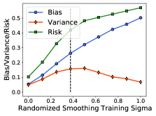
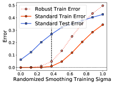
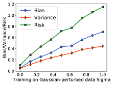
As shown in Figure 3(a), we find that models trained with randomized smoothing behave similarly to adversarially trained models: properties P1-P4 continue to hold. However, for Gaussian-perturbed data the story is different. In Figure 3(b), we see that both the bias and the variance are monotonically increasing as $\sigma^{2}$ increases. Thus, while P1 (monotonic bias) holds, properties P2 and P3 (unimodal variance) do not. This suggests that, in comparison with randomized smoothing, training on Gaussian-perturbed data may not be a good proxy for understanding adversarial training. We summarize the result in the second two rows of Table 1.

(a) Randomized smoothing training.

(b) Training on Gaussian-perturbed data.

Figure 3: Measuring bias/variance/risk and train/test error for randomized smoothing training and training on Gaussian-perturbed data on the CIFAR10 dataset using WRN-28-10, varying $\sigma^{2}$. (a) Results for randomized smoothing training, where the dashed line indicates the robust interpolation threshold. (b) Results for training on Gaussian-perturbed data.

4 Testing Conceptual Models for Adversarial Training

In the previous section, we saw that Gaussian-perturbed data fails to produce the bias-variance properties P1-P3 and thus is not a good model for understanding adversarial training. In this section, we take this idea further, by applying the same test to several other models. We find that we can observe much of the same qualitative behavior already for a linear model adversarially trained on a mixture of Gaussians, as for an adversarially trained neural net on image data. On the other hand, high dimensionality is important–in low dimensions neither of the variance properties (P2 or P3) hold, which casts doubt on some common intuitions around the adversarial generalization gap.

4.1 2D Box Example

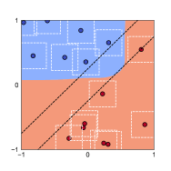
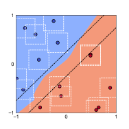
In this subsection, we study the bias-variance decomposition for the “2D box example”. As illustrated in the synthetic binary classification problem of Figure 4(a), “2D box example” visualizes the adversary by adding small $\ell_{\infty}$ boxes around each training sample. Adversarial training then strives to find a decision boundary avoiding the boxes. This model explains the robustness-accuracy gap via the jagged decision boundary. This intuition is commonly presented in the literature (Madry et al., 2017; Wong and Kolter, 2017; Zhang et al., 2019; Yang et al., 2020b) as an important ”mental picture” to understand adversarial training. As we will see, this explanation is limited, and such a low dimensional model fails to capture the complexities of adversarial training.

2D box example experimental setup.

To formally study this 2D box model, we consider a synthetic binary classification problem on $[-1,1]^{2}$, where the input ${\boldsymbol{x}}$ is uniformly sampled from the region $\{{\boldsymbol{x}}\,:\,|x_{1}-x_{2}|\geq\gamma/\sqrt{2}\},$ and the label for ${\boldsymbol{x}}$ is $y=\text{sign}(x_{1}-x_{2})$. Here $\gamma\in(0,1)$ is a margin parameter that controls the distance between two classes. We set the margin $\gamma=1/4$, the number of training sample $n=20$, and the number of test samples as $10,000$. We perform $\ell_{\infty}$ adversarial training using a fully connected network (three hidden layers with 100 nodes each). We vary the adversarial perturbation $\varepsilon$ from $0.0$ to $0.5$, we set the perturbation step size for 10-step-PGD as $\eta=\varepsilon\cdot 0.4$. We use the Adam (Kingma and Ba, 2014) optimizer for 2,000 epochs with a learning rate of 0.001.

(a) Visualization of decision boundaries in 2D.

(b) Bias/variance/risk (box example, $d=2,20$).

Figure 4: (a) Visualization of decision boundaries of $\ell_{\infty}$ adversarially trained models on 2D box example. The training datasets are randomly sampled from the same data distribution. (b) Evaluating the bias, variance, and risk for the $\ell_{\infty}$-adversarial training (with increasing perturbation size) on the box dataset with dimension $d=2$ (left) and $d=20$ (right), and the dashed line indicates the robust interpolation threshold.

Adversarial training on CIFAR10 v.s. 2D box example.

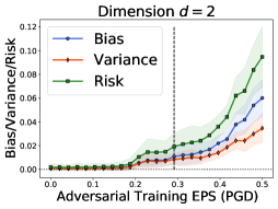
In the left of Figure 4(b) (2D box example), we see that the bias is monotonically increasing and behaves similarly to experiments on real image data, so properties P1 and P4 hold. However, the variance of the 2D box example is different: namely, monotonically increasing instead of unimodal, so P2 and P4 do not hold. This implies that the conceptual “2D box example” is limited for understanding adversarial training.

We offer an intuitive explanation for the monotonically increasing variance for the 2D box example. In this model, larger $\varepsilon$ makes the decision boundary more jagged and complex. In Figure 4(a), we present two random draws of this 2D box example. Although the decision boundaries for different random draws successfully avoid almost all the boxes, the two boundaries are very different, which leads to increased variance.

Higher dimensional box example.

The inconsistent behavior of the variance is partly due to the low dimensionality of the model. We can generalize of the current 2D setting to higher dimensions ($d\gg 2$) by considering data ${\boldsymbol{x}}$ sampled uniformly from $\{{\boldsymbol{x}}\in[-1,1]^{d}\,:\,|\langle{\boldsymbol{x}},\mathbf{1}/\sqrt{d}\rangle|\geq\gamma\}$, and $y=\text{sign}(\langle{\boldsymbol{x}},\boldsymbol{1}\rangle)$. We set the sample size as $n=10\cdot d$ and keep the other parameters fixed. On the left of Figure 4(b), we observe a unimodal variance for a higher dimensional box example, as for the image data. As summarized in the third two rows of Table 1, P1-P4 all hold. The distinction highlights the importance of high-dimensionality of a good conceptual model for adversarial training. We also include results other dimensions in Appendix D.

(a) Bias/variance on MOG.

(b) Error on MOG.

(c) Bias/variance on robust feature distribution.

(d) Error on robust feature distribution.

Figure 5: (a)(b): Bias, variance and training error for adversarial logistic regression with mixture of Gaussian (MoG) data. (c)(d): Bias, variance and training error for adversarial logistic regression with the robust feature distribution described in Eq. (6). For all four figures, the dashed line indicates robust interpolation threshold.

4.2 Logistic Regression

Our investigation of the 2D box example leads us to consider an intrinsically high dimensional model. In this section, we consider a standard logistic regression setup with adversarial training.

Adversarial logistic regression.

We use the standard cross-entropy loss for logistic regression

$${\textsf{R}}^{(n)}({\boldsymbol{\theta}})=\frac{1}{n}\sum_{i=1}^{n}\ell(y_{i}\langle{\boldsymbol{x}}_{i},{\boldsymbol{\theta}}\rangle),$$

where $\ell(z)=\log(1+e^{-z})$. The inner maximization problem (using $\ell_{2}$ perturbation of magnitude $\varepsilon$) in the adversarial loss can be solved exactly (and is often used for theoretical analysis (Javanmard et al., 2020; Javanmard and Soltanolkotabi, 2020; Dobriban et al., 2020)):

$${\textsf{ARisk}}^{(n)}({\boldsymbol{\theta}})=\frac{1}{n}\sum_{i=1}^{n}\max_{\|{\boldsymbol{\delta}}_{i}\|_{2}\leq\varepsilon}\ell(y_{i}\langle{\boldsymbol{x}}_{i},{\boldsymbol{\theta}}\rangle)=\frac{1}{n}\sum_{i=1}^{n}\log\left(1+e^{-y_{i}\langle{\boldsymbol{x}}_{i},{\boldsymbol{\theta}}\rangle+\varepsilon\|{\boldsymbol{\theta}}\|_{2}}\right).$$ (4)

Adversarial training amounts to solving the convex program $\hat{{\boldsymbol{\theta}}}_{n}=\arg\min_{{\boldsymbol{\theta}}}{\textsf{ARisk}}^{(n)}({\boldsymbol{\theta}}).$ Given a test data-point $({\boldsymbol{x}},y)$, the risk is ${\textsf{R}}(\hat{{\boldsymbol{\theta}}}_{n})=\mathbb{E}_{{\boldsymbol{x}},y}\,\ell(y\langle\hat{{\boldsymbol{\theta}}}_{n},{\boldsymbol{x}}\rangle)$. Instead of the bias-variance decomposition for the squared loss used in other sections, we use a bias-variance decomposition for logistic loss introduced in E, which is more natural for logistic regression. We will study two distributions for the underlying data $({\boldsymbol{x}},y)$.

Mixture of Gaussians.

As studied in previous works (Dobriban et al., 2020; Javanmard and Soltanolkotabi, 2020), we assume that, for $i=1,\dots,n$, each pair of training samples ${\boldsymbol{x}}_{i}\in{\mathbb{R}}^{d}$ and $y_{i}\in\{-1,1\}$ has distribution

$$y\overset{\text{u.a.r}}{\sim}\{-1,+1\},\quad{\boldsymbol{x}}_{i}|y_{i}\sim{\mathcal{N}}(y_{i}{\boldsymbol{v}},\sigma^{2}{\boldsymbol{I}}_{d}),$$ (5)

where ${\boldsymbol{v}}=[1,1,\dots,1]/\sqrt{d}\in{\mathbb{R}}^{d}$ specifies the center of the cluster. For this experiment, we set the number of training samples $n=100$, the data dimension $d=100$, and the cluster radius (variance of the Gaussian mixture) $\sigma=0.7$.

Planted robust feature distribution.

To investigate whether the observed bias-variance behavior in adversarial logistic regression is tied to the the specific mixture-of-Gaussians, we also consider a different distribution proposed in Tsipras et al. (2018). For a data-label pair $({\boldsymbol{x}},y)$, we let

$$y\overset{\text{u.a.r}}{\sim}\{-1,+1\},~{}~{}{\boldsymbol{x}}_{1}=\begin{cases}+y,&\text{w.p. }0.95\\ -y,&\text{w.p. }0.05\end{cases},~{}~{}({\boldsymbol{x}}_{2},\dots,{\boldsymbol{x}}_{d})\overset{\text{i.i.d}}{\sim}{\mathcal{N}}(y{\boldsymbol{v}},{\boldsymbol{I}}_{d-1}),$$ (6)

where ${\boldsymbol{v}}=[1,1,\dots,1]/\sqrt{d}\in{\mathbb{R}}^{d-1}$. In this model , an additional robust feature is added to the first coordinate of the of the feature vector ${\boldsymbol{x}}_{1}$ and the rest of the coordinates are sampled from a mixture of Gaussians. The first coordinate ${\boldsymbol{x}}_{1}$ can be interpreted as the “robust feature” since it is hard to be perturbed. Meanwhile, the robust feature is less accurate because itself can only provide $95\%$ accuracy. More details discussions on the trade-off between robustness and accuracy can be found in Tsipras et al. (2018). We set the dimension $d=100$ and the number of training samples $n=150$.

Results.

Results for both models are depicted in Figure 5(a). In both cases we see that properties P2 and P3 hold–the variance increases and then decreases with $\varepsilon$, and the peak occurs at the robust interpolation threshold. P4 also holds–the bias dominates the variance. However, P1 does not quite hold–the bias initially decreases at the start of training before eventually increasing. We believe the slight decrease in bias is attributable to the exceeding simplicity of probabilistic model for the data. For both distributions, the linear classifiers are already optimal in the population. Therefore slightly increasing $\varepsilon$ does not lead to a qualitatively incorrect decision boundary as it could for deep neural networks on images. However for large enough $\varepsilon$ the bias still increases as expected. We summarize the results in the last two rows of Table 1.

(a) Standard bias-variance.

(b) Adversarial bias-variance.

(c) Standard and robust error.

Figure 6: Results of adversarial training on CIFAR10 ($\ell_{\infty},\varepsilon=8/255$) for four different methods: [Standard] – standard adversarial training; [More data] – using additional unlabeled data; [Pre-training] – applying adversarial pre-trained model; [More data]+[Pre-training] – using both additional unlabeled data and adversarial pre-training. Points toward lower left indicate better performance in all three figures.

Figure 7: Measuring performance for $(\ell_{\infty},\varepsilon=8/255)$-adversarial training (with increasing width factor for WideResNet-28-[width]) on CIFAR10 dataset. (left) Evaluating bias, variance, and risk. (right) Evaluating robust training error and standard training/test error. The dashed line indicates the robust interpolation threshold.

5 Analyzing Model Performance via the Bias-Variance Decomposition

In this section, we apply the bias-variance decomposition to analyze the performance of adversarially trained models. We measure the bias and variance of techniques that improve the performance of adversarial training, including using additional unlabeled data (Carmon et al., 2019) and adversarial pre-training (Hendrycks et al., 2019a). We also study the bias-variance decomposition for $\ell_{\infty}$-adversarially trained models with different width factors. Our motivation is to understand whether these techniques can reduce the bias, since that is the dominant term in the risk, and the previously considered early stopping technique primarily reduces variance.

Analyzing techniques that improve adversarial training.

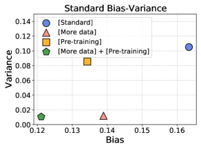
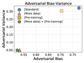
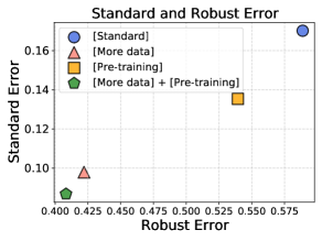
Additional unlabeled data and adversarial pre-training can improve model performance for both standard and robust accuracy (Carmon et al., 2019; Hendrycks et al., 2019a; Salman et al., 2019; Gowal et al., 2020). We consider the same Wide-ResNet architecture (WRN-28-10) as before, trained at $\varepsilon=8/255$ in $\ell_{\infty}$-norm. We investigate four cases: (1). Standard adversarial training; (2). Using additional unlabeled data; (3). Using adversarially pre-trained models for initialization; (4). Using both additional unlabeled data and adversarial pre-training. We measure the standard bias and variance, their adversarial counterparts (see Section A), and the standard and robust test errors in each case. The results are summarized in Figure 6.

In Figure 6(a), we see that additional unlabeled data significantly decreases both the bias and variance, while pre-training mainly decreases the bias. Using both a pre-trained model and additional data further decreases the bias, leading to a smaller clean error (see Figure 6(c)). In terms of the adversarial bias-variance decomposition results shown in Figure 6(b), we find that adversarial pre-training mainly improves the adversarial bias term, and additional unlabeled data improves both the adversarial bias and adversarial variance.

Model width.

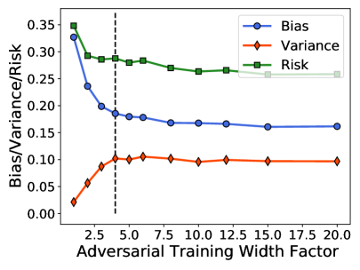
We also consider increasing the width factor of the network, training WRN-28-$[\textit{width}]$ for $\textit{width}\in\{1,\cdots,20\}$. From Figure 7, we find that making models wider only marginally improves the bias beyond a certain width factor. This suggest that increasing width might not be a scalable solution to reduce the generalization gap in adversarial training.

Aside from width, previous works demonstrate that making models deeper can significantly improve generalization in adversarial training (Xie et al., 2019; Gowal et al., 2020). We hypothesize that using deeper models might be more effective than increasing width, and that they would decrease bias. This would align with results for regularly trained models (Yang et al., 2020), for which deeper models decreased bias at the cost of variance.

6 Discussion and Future Work

In this paper, we studied the generalization gap in adversarial training by measuring the bias and variance of adversarially trained models. Across many training settings, we robustly observed that the bias increases monotonically (P1) with the adversarial perturbation radii $\varepsilon$ and is the dominant term of the risk (P4). The variance is unimodal (P2) with its peak near the robust interpolation threshold (P3). Beyond their intrinsic interest, P1-P4 allowed us to test several conceptual models for the generalization gap and thus obtain new insights into its underlying cause. We further used bias and variance to study how existing techniques have helped reduce the generalization gap.

Implications for adversarial training.

Our results provide a jumping-off point for reducing the adversarial generalization gap. They show that the gap is mainly due to bias, pinpointing the locus for improvement. The large bias may be counterintuitive, as it occurs even when the training error is zero, which usually instead corresponds to low bias and high variance. This suggests that adversarial training imposes a strong form of implicit regularization (Neyshabur et al., 2014) that causes the bias. A better understanding of this regularization could perhaps help us design better architectures to accommodate adversarial training.

Variance peak and interpolation threshold.

Our variance curves consistently reach their maximum near the point where the robust training error becomes non-zero. This echoes results in Yang et al. (2020), who found a parallel phenomenon for regular training with models of increasing width. Their bias/variance-width plot aligns with our bias/variance-$\varepsilon$ plot. In both cases, the variance is unimodal with peak near the interpolation threshold. The connection here is perhaps deeper: Increasing width increases model complexity and increasing $\varepsilon$ adds regularization, which effectively reduces model complexity. This explains why we observe bias/variance behavior in reverse (increased bias in $\varepsilon$ vs. decreased bias in width). The connection hints to a universal behavior of the model variance in relation to a notion of “effective model complexity”, and deserves refined investigation in future work.

Appendix A Adversarial Bias-variance Decomposition

In this section, we propose a generalized bias-variance decomposition, the adversarial bias-variance decomposition, to help us investigate the behavior of adversarial trained models evaluated on adversarial examples. A challenge is that in the adversarial setting, we not only need to take into account the prediction at a particular test point ${\boldsymbol{x}}$, but also at a point ${\boldsymbol{x}}^{\prime}={\boldsymbol{x}}+{\boldsymbol{\delta}}$, where ${\boldsymbol{\delta}}\in\Delta$ is the adversarial perturbation.

For a robust model, $f_{\widehat{{\boldsymbol{\theta}}}({\mathcal{T}})}\left({\boldsymbol{x}}+{\boldsymbol{\delta}}({\boldsymbol{x}},{\boldsymbol{y}},{\mathcal{T}})\right)$ should still be a good predictor of the label $y$. Therefore, as in the standard training setting, the prediction $f_{\widehat{{\boldsymbol{\theta}}}}\left({\boldsymbol{x}}+{\boldsymbol{\delta}}({\boldsymbol{x}},{\boldsymbol{y}},{\mathcal{T}})\right)$ should not depend too much on ${\mathcal{T}}$. We can measure how much the prediction depends on ${\mathcal{T}}$ by computing the adversarial variance ${\textsf{AVar}}=\mathbb{E}_{{\boldsymbol{x}},{\boldsymbol{y}}}\text{Var}_{{\mathcal{T}}}[f_{\widehat{{\boldsymbol{\theta}}}({\mathcal{T}})}({\boldsymbol{x}}+{\boldsymbol{\delta}}({\boldsymbol{x}},{\boldsymbol{y}},{\mathcal{T}}))]$. The adversarial bias can be analogously defined as ${\textsf{ABias}}=\mathbb{E}_{{\boldsymbol{x}},{\boldsymbol{y}}}[\|{\boldsymbol{y}}-\mathbb{E}_{\mathcal{T}}f_{\widehat{{\boldsymbol{\theta}}}({\mathcal{T}})}({\boldsymbol{x}}+{\boldsymbol{\delta}}({\boldsymbol{x}},{\boldsymbol{y}},{\mathcal{T}}))\|^{2}]$. One can check that the sum of adversarial bias (ABias) and adversarial variance (AVar) gives the expected adversarial risk (ARisk), i.e.,

$${\textsf{ARisk}}=\mathbb{E}_{{\mathcal{T}}}\mathbb{E}_{{\boldsymbol{x}},{\boldsymbol{y}}}\big{[}\max_{{\boldsymbol{\delta}}\in\Delta}\big{\|}f_{\widehat{{\boldsymbol{\theta}}}}({\boldsymbol{x}}+{\boldsymbol{\delta}})-{\boldsymbol{y}}\big{\|}^{2}\big{]}={\textsf{ABias}}+{\textsf{AVar}},$$ (7)

where ${\boldsymbol{\delta}}_{{\mathcal{T}}}$ is short for ${\boldsymbol{\delta}}({\boldsymbol{x}},{\boldsymbol{y}},{\mathcal{T}})$. The advantage of our definition of variance is that it directly measures the variation of the model’s prediction at test sample ${\boldsymbol{x}}$ in presence of adversarial perturbation. An algorithm for estimating the variance given a single training dataset ${\mathcal{T}}$ at a particular test point $({\boldsymbol{x}},{\boldsymbol{y}})$ is given in Algorithm 1 in Appendix B.

In addition to standard bias-variance decomposition, we also study the adversarial bias-variance decomposition (defined in Eq. (7)) for adversarial training and randomized smoothing training on the CIFAR10 dataset. We apply the same training dataset partition procedure as bias-variance decomposition. To approximately find ${\boldsymbol{\delta}}_{{\mathcal{T}}}$ defined in Eq. (7), we use the $\ell_{\infty}$-PGD adversarial attack for generating the adversarial perturbations, where the number of perturbation steps is 20 and the step size is $\eta=0.15\cdot(\varepsilon/255)$.

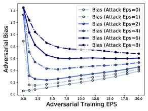
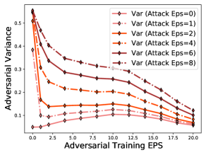
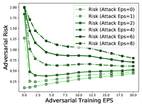
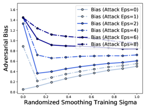
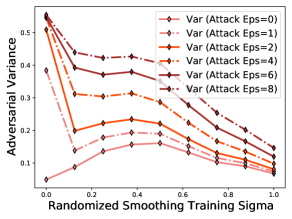
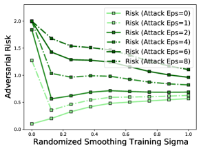
The results for the $\ell_{\infty}$ adversarially trained models are summarized in Figure 8. With increasing perturbation size for evaluating the adversarial bias and variance, the adversarial bias curve is changed from monotone increasing to monotone decreasing, and the variance curve is changed from unimodal to monotone decreasing. The adversarial variance is relatively small compared with the adversarial bias under various attack radii; similar to the standard bias-variance results in Figure 1. Furthermore, from Figure 9, we observe that models trained with randomized smoothing have similar characteristic adversarial bias-variance curve shapes as adversarially trained models (in Figure 8): the adversarial variance under all adversarial perturbations becomes smaller when increasing the training variance $\sigma^{2}$, and the bias shape is changed from monotone increasing to monotone decreasing with increased adversarial perturbation $\varepsilon$.

Figure 8: Adversarial bias, variance, and risk for $\ell_{\infty}$ adversarially trained models on the CIFAR10 dataset using WRN-28-10. Each curve corresponds to the $\varepsilon$-adversarial bias-variance decomposition, and the EPS represents the $\ell_{\infty}=\textsf{EPS}/255.0$ PGD attack. (Left) Adversarial bias. (Middle) Adversarial variance. (Right) Adversarial risk.

Figure 9: Adversarial bias, variance, and risk for randomized smoothing training models on the CIFAR10 dataset using WRN-28-10. Each curve corresponds to the $\varepsilon$-adversarial bias-variance decomposition, and the EPS represents the $\ell_{\infty}=\textsf{EPS}/255.0$ PGD attack. (Left) Adversarial bias. (Middle) Adversarial variance. (Right) Adversarial risk.

Appendix B Algorithm for Estimating Bias-variance

In this section, we present the algorithm for estimating the (adversarial) variance for squared loss. Also, we introduce the adversarial bias-variance decomposition for cross-entropy loss.

B.1 Algorithm for Estimating the Variance

The algorithm for estimating the variance is described in Algorithm 1. The adversarial variance and bias can be estimated as follows:

$$\widehat{\textsf{AVar}} =\mathbb{E}_{{\boldsymbol{x}},{\boldsymbol{y}}}\left[\widehat{\textsf{AVar}}({\boldsymbol{x}},{\boldsymbol{y}})\right],$$ (8)

$$\widehat{\textsf{ABias}} =\frac{1}{K}\sum_{k=1}^{K}\mathbb{E}_{{\mathcal{T}}^{(k)}}\mathbb{E}_{{\boldsymbol{x}},{\boldsymbol{y}}}\left[\max_{{\boldsymbol{\delta}}\in\Delta}\left\|f_{\widehat{{\boldsymbol{\theta}}}({\mathcal{T}}^{(k)})}({\boldsymbol{x}}+{\boldsymbol{\delta}})-{\boldsymbol{y}}\right\|^{2}\right]-\widehat{\textsf{AVar}},$$

where $\widehat{\textsf{AVar}}({\boldsymbol{x}},{\boldsymbol{y}})$ is calculated by Algorithm 1. We can also apply Eq. (8) for evaluating the standard bias and variance by setting $\varepsilon=0$ for the perturbation set $\Delta=\{{\boldsymbol{\delta}}:\|{\boldsymbol{\delta}}\|_{p}\leq\varepsilon\}$.

Algorithm 1 Estimating Adversarial Variance for Squared Loss

  Input: Test point $({\boldsymbol{x}},\ {\boldsymbol{y}})$, Training set ${\mathcal{T}}$, Number of repetitions $K$.

  for $k=1$ to $K$ do

     Split ${\mathcal{T}}$ into ${\mathcal{T}}_{1}^{(k)},\dots,{\mathcal{T}}_{N}^{(k)}$.

     for $j=1$ to $N$ do

        Perform adversarial training on training dataset ${\mathcal{T}}_{j}^{(k)}$;

        Find $\hat{{\boldsymbol{\theta}}}({\mathcal{T}}_{j}^{(k)})$ that approximately solves

$$\min_{{\boldsymbol{\theta}}}\frac{1}{|{\mathcal{T}}_{j}^{(k)}|}\sum_{i\in{\mathcal{T}}_{j}^{(k)}}\max_{{\boldsymbol{\delta}}_{i}\in\Delta}\,\ell(f_{{\boldsymbol{\theta}}}({\boldsymbol{x}}_{i}+{\boldsymbol{\delta}}_{i}),{\boldsymbol{y}}_{i});$$

        Find adversarial perturbation ${\boldsymbol{\delta}}({\boldsymbol{x}},{\boldsymbol{y}},{\mathcal{T}}_{j}^{(k)})$ that approximately solves

$$\max_{{\boldsymbol{\delta}}\in\Delta}\ell\Big{(}f_{\hat{{\boldsymbol{\theta}}}({\mathcal{T}}_{j}^{(k)})}({\boldsymbol{x}}+{\boldsymbol{\delta}}),{\boldsymbol{y}}\Big{)};$$

     end for

  end for

  for $k=1$ to $K$ do

     Compute

$$\widehat{\textsf{AVar}}({\boldsymbol{x}},{\boldsymbol{y}},{\mathcal{T}}^{(k)})$$

$$= \frac{1}{N-1}\sum_{j=1}^{N}\Big{\|}f_{\hat{{\boldsymbol{\theta}}}({\mathcal{T}}_{j}^{(k)})}({\boldsymbol{x}}+{\boldsymbol{\delta}}({\boldsymbol{x}},{\boldsymbol{y}},{\mathcal{T}}_{j}^{(k)}))-{\frac{1}{N}\sum_{j=1}^{N}f_{\hat{{\boldsymbol{\theta}}}({\mathcal{T}}_{j}^{(k)})}({\boldsymbol{x}}+{\boldsymbol{\delta}}({\boldsymbol{x}},{\boldsymbol{y}},{\mathcal{T}}_{j}^{(k)}))}\Big{\|}_{2}^{2};$$

  end for

  Compute $\widehat{\textsf{AVar}}({\boldsymbol{x}},{\boldsymbol{y}})=\frac{1}{K}\sum_{k=1}^{K}\widehat{\textsf{AVar}}({\boldsymbol{x}},{\boldsymbol{y}},{\mathcal{T}}^{(k)})$.

B.2 Bias-variance Decomposition for Cross-entropy Loss

Inspired by Pfau [2013], Yang et al. [2020] provides a bias-variance decomposition for cross-entropy loss. We also extend their decomposition to the adversarial setting. We use boldface ${\boldsymbol{f}}$ instead of $f$ to emphasize that ${\boldsymbol{f}}_{{\boldsymbol{\theta}}}\in{\mathbb{R}}^{c}$ is now a vector that represents a probability distribution over the class labels, i.e., $\sum_{i=1}^{c}{\boldsymbol{f}}_{\boldsymbol{\theta}}({\boldsymbol{x}})_{i}=1$. We are given a trained model $\hat{{\boldsymbol{\theta}}}({\mathcal{T}})$, a test point $({\boldsymbol{x}},{\boldsymbol{y}})\in{\mathbb{R}}^{d}\times{\mathbb{R}}^{c}$, where ${\boldsymbol{y}}$ is the one-hot encoding of the class membership of input ${\boldsymbol{x}}$. We first compute the worst-case perturbation as

$${\boldsymbol{\delta}}({\boldsymbol{x}},{\boldsymbol{y}},{\mathcal{T}})\in\arg\max_{{\boldsymbol{\delta}}\in\Delta}\left\{H({\boldsymbol{f}}_{\hat{{\boldsymbol{\theta}}}}({\boldsymbol{x}}+{\boldsymbol{\delta}}),{\boldsymbol{y}})\right\},$$

where $H({\boldsymbol{a}},{\boldsymbol{b}})=-\sum_{i=1}^{c}{\boldsymbol{a}}_{i}\log({\boldsymbol{b}}_{i})$ is the standard cross-entropy loss. At the adversarially perturbed test point ${\boldsymbol{x}}^{\prime}={\boldsymbol{x}}^{\prime}({\boldsymbol{x}},{\boldsymbol{y}},{\mathcal{T}})={\boldsymbol{x}}+{\boldsymbol{\delta}}({\boldsymbol{x}},{\boldsymbol{y}},{\mathcal{T}})$, we define the average prediction $\overline{{\boldsymbol{f}}}$ at ${\boldsymbol{x}}^{\prime}$ as

$$\overline{{\boldsymbol{f}}}_{i}\propto\exp\left[\mathbb{E}_{{\mathcal{T}}}\log{\boldsymbol{f}}_{\hat{{\boldsymbol{\theta}}}}({\boldsymbol{x}}^{\prime})_{i}\right],~{}~{}i\in[c],~{}~{}\text{and}~{}~{}\sum_{i=1}^{c}\overline{{\boldsymbol{f}}}_{i}=1.$$

Now we are ready to state the formula for the adversarial “bias-variance” decomposition of the cross-entropy loss:

$$\underbrace{\mathbb{E}_{{\mathcal{T}}}\mathbb{E}_{{\boldsymbol{x}},{\boldsymbol{y}}}\left[\max_{{\boldsymbol{\delta}}\in\Delta}H\left(f_{\hat{{\boldsymbol{\theta}}}({\mathcal{T}})}({\boldsymbol{x}}+{\boldsymbol{\delta}}),{\boldsymbol{y}}\right)\right]}_{\textsf{Adversarial Risk (CE)}}$$ (9)

$$= \mathbb{E}_{{\boldsymbol{x}},{\boldsymbol{y}}}\mathbb{E}_{{\mathcal{T}}}H\left(f_{\hat{{\boldsymbol{\theta}}}({\mathcal{T}})}({\boldsymbol{x}}+{\boldsymbol{\delta}}({\boldsymbol{x}},{\boldsymbol{y}},{\mathcal{T}})),{\boldsymbol{y}}\right)+\underbrace{\mathbb{E}_{{\boldsymbol{x}},{\boldsymbol{y}}}D_{\textsf{KL}}\left({\boldsymbol{y}}\|\overline{{\boldsymbol{f}}}\right)}_{\textsf{Adversarial Bias (CE)}}.$$

The standard bias and variance can be computed analogously.

Appendix C Additional Experiments for Deep Neural Networks

In this section, we provide additional experimental results details related to Section 3. Specifically, we provide the detailed experimental setup for Gaussian noise training in Section C.1. In Section C.2, we present additional experimental results for the $\ell_{2}$ and $\ell_{\infty}$ adversarial training on CIFAR10, CIFAR100, and ImageNet10 datasets. We also study the effect of the width factor in adversarial training in Section C.2. In Section C.3, we study the bias and variance of deep models on out-of-distribution (OOD) datasets. In Section C.4, we evaluate the cross-entropy loss bias and variance for $\ell_{\infty}$ and $\ell_{2}$ adversarially trained models on the CIFAR10 dataset.

C.1 Experimental setup for training with Gaussian Noise

Experimental setup.

For randomized smoothing training, following previous works Lecuyer et al. [2019], Cohen et al. [2019], we train the models with additive Gaussian data augmentation with variance $\sigma^{2}$ on the CIFAR10 dataset. The variance $\sigma^{2}$ is chosen as $\sigma\in\{k\cdot 0.125\,:\,k=0,\dots,8\}$. After adding noise to the input, we clip the pixels to $[0.0,1.0]$. For training on Gaussian-perturbed data, we perturb the training images from CIFAR10 with random additive Gaussian noise with variance $\sigma^{2}$, where $\sigma\in\{k\cdot 0.125\,:\,k=0,\dots,8\}$, then clip pixels to $[0.0,1.0]$ and save the images using the standard JPEG compression. The same architecture (WRN-28-10) and optimization procedure are applied for randomized smoothing training and training on Gaussian-perturbed data as for $\ell_{\infty}$ adversarial training, described earlier. The robust error (in Figure 3(a)) of randomized smoothing trained models is evaluated by adding random Gaussian noise (with the same variance $\sigma^{2}$ as in training) to the training dataset.

C.2 Additional Experiments on Measure Bias-variance of Adversarial Training models on CIFAR10/100 and ImageNet10

For $\ell_{2}$ adversarial training, we apply a 10-step $(\ell_{2})$ PGD attack with perturbation step size $\eta=0.25\cdot(\varepsilon/255)$.

$\ell_{2}$ adversarial training on CIFAR10.

We first study the bias-variance decomposition of $\ell_{2}$ adversarially trained models on the CIFAR10 dataset. We summarize the results in Figure 10. The bias and variance of $\ell_{2}$ adversarially trained models are similar to the ones in $\ell_{\infty}$ adversarial training (in Figure 1). We find that the variance is unimodal and the bias is monotonically increasing with the perturbation size. Also, the variance peak is near the robust interpolation threshold. In summary, we observe properties P1-P4 for $\ell_{2}$ adversarial training on CIFAR10.

Results on CIFAR100.

In Figure 11 and Figure 12, we study the bias-variance behavior on the CIFAR100 dataset. Following Rice et al. [2020], we use pre-activation ResNet18 (PreResNet-18) architecture for the CIFAR100 dataset and apply the same training parameters as used for CIFAR10. We find that, on the CIFAR100 dataset, the variance is indeed unimodal, the bias dominates the risk and monotonically increasing, and the peak of the variance is close to the robust interpolation threshold. Similar to the results on CIFAR10, we observe properties P1-P4 for $\ell_{2}$ and $\ell_{\infty}$ adversarial training on CIFAR100.

Results on ImageNet10.

In Figure 13, we study the bias-variance behavior on the ImageNet10 dataset. We use the standard ResNet18 architecture for the ImageNet10 dataset. We apply the hyperparameters for adversarial training as in the CIFAR10/100 dataset. As shown in Figure 13, We find that the variance is unimodal and the bias is monotonically increasing dominates the risk and monotonically increasing, and the peak of the variance is close to the robust interpolation threshold. In summary, we observe properties P1-P4 for $\ell_{\infty}$ adversarial training on ImageNet10.

Effect of width factor.

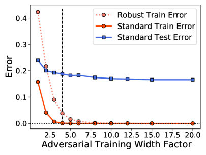
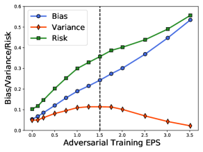
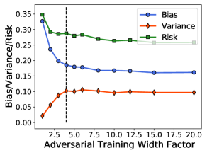
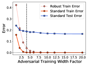
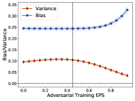
We study the effect of the width factor of the WideResNet-28 in $(\ell=8.0/255.0)$ adversarial training on the CIFAR10 dataset. We apply the same training parameters as mentioned in Section 3.1 and only change the wide factor of WideResNet-28 from 1 to 20. As shown in Figure 14, the variance changes monotonicity at the interpolation threshold (width=4). We observe that the bias is monotonically decreasing with the width factor. The variance is increasing before the robust interpolation threshold. After the threshold, the variance value does not change too much.

Figure 10: Measuring performance for $(\ell_{2}=\varepsilon)$-adversarial training (with increasing perturbation size) on CIFAR10 dataset. (left) Evaluating bias, variance, and risk for the $\ell_{2}$-adversarially trained models (WideResNet-28-10) on the CIFAR10 dataset. (right) Evaluating robust training error, standard training/test error for the $\ell_{2}$-adversarially trained models (WideResNet-28-10) on the CIFAR10 dataset.

Figure 11: Measuring performance for $(\ell_{\infty}=\varepsilon/255.0)$-adversarial training (with increasing perturbation size) on CIFAR100 dataset. (left) Evaluating bias, variance, and risk for the $\ell_{\infty}$-adversarially trained models (PreResNet-18) on the CIFAR100 dataset. (right) Evaluating robust training error, standard training/test error for the $\ell_{\infty}$-adversarially trained models (PreResNet-18) on the CIFAR100 dataset.

Figure 12: Measuring performance for $(\ell_{2}=\varepsilon)$-adversarial training (with increasing perturbation size) on CIFAR100 dataset. (left) Evaluating bias, variance, and risk for the $\ell_{2}$-adversarially trained models (PreResNet-18) on the CIFAR100 dataset. (right) Evaluating robust training error, standard training/test error for the $\ell_{2}$-adversarially trained models (PreResNet-18) on the CIFAR100 dataset.

Figure 13: Measuring performance for $(\ell_{\infty}=\varepsilon/255.0)$-adversarial training (with increasing perturbation size) on ImageNet10 dataset. (left) Evaluating bias, variance, and risk for the $\ell_{\infty}$-adversarially trained models (ResNet-18) on the ImageNet10 dataset. (right) Evaluating robust training error, standard training/test error for the $\ell_{\infty}$-adversarially trained models (ResNet-18) on the ImageNet10 dataset.

Figure 14: Measuring performance for $(\ell_{\infty}=8.0/255.0)$-adversarial training (with increasing width factor for WideResNet-28-[width]) on CIFAR10 dataset. (left) Evaluating bias, variance, and risk for the $(\ell_{\infty}=8.0/255.0)$-adversarially trained models (WideResNet-28-[width]) on the CIFAR10 dataset. (right) Evaluating robust training error, standard training/test error for the $\ell_{\infty}$-adversarially trained models (WideResNet-28-[width]) on the CIFAR10 dataset.

Figure 15: Bias, variance, and risk for $\ell_{\infty}$-adversarial training models evaluated on the CIFAR10-C dataset with different severity. Each curve corresponds to one level of severity, and severity=0 corresponds to the standard test CIFAR10 testset. (Left) Bias. (Middle) Variance. (Right) Risk.

C.3 Measuring Bias-variance of Adversarial Training Models on OOD datasets.

Adversarial training evaluated on OOD data.

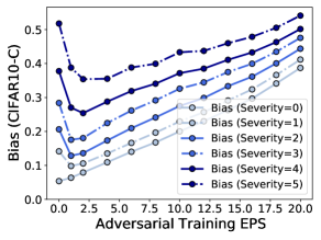
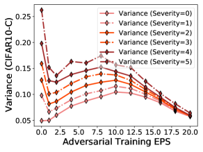
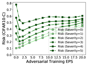
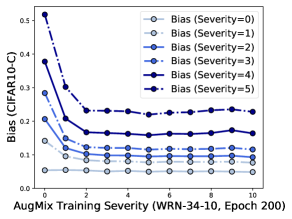
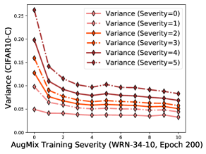
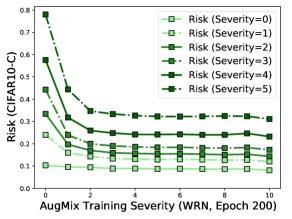
We evaluate the bias, variance, and risk of the adversarially trained models with various $\ell_{\infty}$ perturbation radii on the CIFAR10-C dataset. CIFAR10-C contains 15 different common corruptions with five levels of severity, where samples with larger severity level are generally harder to classify. We evaluate the bias and variance on test samples with various severity levels. The results are summarized in Figure 15.

We observe that the bias curve becomes U-shaped on CIFAR10-C and the variance curve changes to a “double-descent-shaped” curve (with two dips) when evaluated on OOD data. Another intriguing observation is that when the adversarial perturbation radius $\varepsilon$ is small, both the bias and the variance (evaluated on OOD data) of the adversarially trained models are smaller than for models with standard training ($\varepsilon=0$). This suggests that $\ell_{\infty}$ adversarial training with small perturbation radii improves model performance (in terms of both bias and variance) on common corruptions, which aligns well with findings in Kireev et al. [2021]. It would be a valuable direction for future work to explore how to better trade off bias and variance of adversarially trained models for better OOD generalization.

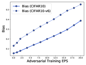
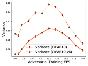
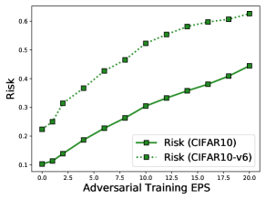
We also study the bias-variance decomposition for $\ell_{\infty}$-adversarially trained models and AugMix Hendrycks et al. [2019b]-trained models (on the CIFAR10 dataset) evaluated on datasets under distributional shift. This includes natural distributional shift, in the CIFAR10-v6 dataset Recht et al. [2018], and a common corruption benchmark, the CIFAR10-C dataset Hendrycks and Dietterich [2019].

CIFAR10-v6 results.

CIFAR10-v6 contains new collected test images for the CIFAR10 dataset. The results of $\ell_{\infty}$-adversarial training on CIFAR10-v6 are summarized in Figure 16. We find that the bias and variance on CIFAR10-v6 are similar to the standard test dataset case (in Figure 1), whereas the variance decreases after $\varepsilon=10$.

AugMix training.

In addition, we study the bias-variance decomposition for AugMix training on the CIFAR10 dataset. We change the severity (augmentation severity parameter in AugMix) from 0 to 10, where 0 corresponds to the standard training and 10 is the maximum severity defined in AugMix. We summarize the bias-variance decomposition results in Figure 17. For AugMix training, we find that bias, variance, and risk are monotonically decreasing with increased augmentation severity. The bias-variance behavior of AugMix training is different from $\ell_{\infty}$-adversarial training (in Figure 15).

Figure 16: Compare bias, variance, and risk for $\ell_{\infty}$-adversarial training models evaluated on the CIFAR10-v6 and standard CIFAR10 testset. (Left) Bias. (Middle) Variance. (Right) Risk.

Figure 17: Bias, variance, and risk for AugMix training models (without applying JSD loss) evaluated on the CIFAR10-C dataset with different severity. Each curve corresponds to one level of severity, and severity=0 corresponds to the standard test CIFAR10 testset. (Left) Bias. (Middle) Variance. (Right) Risk.

C.4 Measuring Bias-variance Decomposition for Cross-Entropy Loss.

We study the bias-variance decomposition for cross-entropy (CE) loss defined above. We follow Algorithm 1 in Yang et al. [2020] to evaluate the bias and variance for the cross-entropy loss. Specifically, we evaluate the (cross-entropy loss) bias-variance decomposition for $\ell_{\infty}$-adversarially trained models (as shown in Figure 18) and $\ell_{2}$-adversarially trained models (shown in Figure 19) on the CIFAR10 dataset. From Figure 18 and Figure 19, we observe the unimodal variance curve and monotonically increasing bias curve for the (cross-entropy loss) bias-variance decomposition. The peak of the (cross-entropy loss) variance is also near the robust interpolation threshold.

Figure 18: Measuring performance for $(\ell_{\infty}=\varepsilon/255.0)$-adversarial training (with increasing perturbation size) on CIFAR10 dataset. (left) Evaluating (cross-entropy loss) bias, variance, and risk for the $\ell_{\infty}$-adversarially trained models (WideResNet-28-10) on the CIFAR10 dataset. (right) Evaluating robust training error, standard training/test error for the $\ell_{\infty}$-adversarially trained models (WideResNet-28-10) on the CIFAR10 dataset.

Figure 19: Measuring performance for $(\ell_{2}=\varepsilon)$-adversarial training (with increasing perturbation size) on CIFAR10 dataset. (left) Evaluating (cross-entropy loss) bias, variance, and risk for the $\ell_{2}$-adversarially trained models (WideResNet-28-10) on the CIFAR10 dataset. (right) Evaluating robust training error, standard training/test error for the $\ell_{2}$-adversarially trained models (WideResNet-28-10) on the CIFAR10 dataset.

Appendix D Additional Experiments on Simplified Models

In this section, we present additional experiments on 2D box example and adversarial logistic regression as described in Section 4.

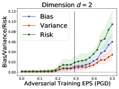
First of all, we present the bias-variance experimental results on 2D box example with different dimension $(2\leq d\leq 50)$ in Figure 20. Regarding the experimental setup, we only change the dimension $d$, and the number of training samples $n=10\cdot d$ (i.e., same setup as described in Section 4.1).

(a) $d=2$

(b) $d=3$

(c) $d=4$

(d) $d=5$

(e) $d=6$

(f) $d=7$

(g) $d=8$

(h) $d=9$

(i) $d=10$

(j) $d=15$

(k) $d=20$

(l) $d=25$

(m) $d=30$

(n) $d=40$

(o) $d=50$

Figure 20: Bias-variance behavior of adversarial training on the box dataset with different dimensions ($d\in\{2,\cdots,50\}$).

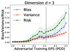
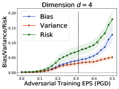
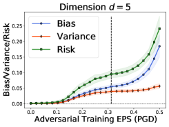
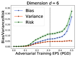
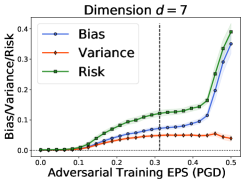
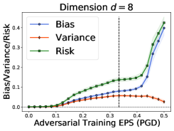
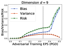
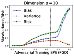
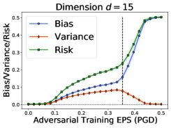
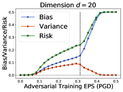
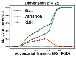
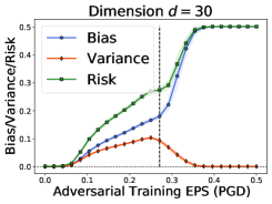
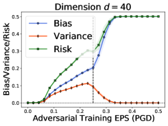
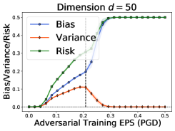
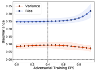
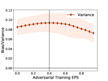
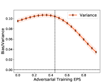
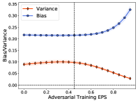
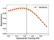
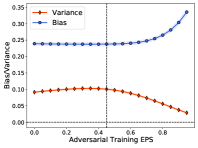
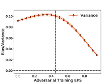
Secondly, we present additional experiments on adversarial logistic regression. The precise setup of the experiments is defined in Section 4. We consider $d\in\{10,20,50,100,200,500\}$ and $n=d$ for the adversarial logistic regression. As shown in Figure 21, the variance is unimodal and the variance peak is close to the interpolation threshold.

(a) $n=10,d=10,\sigma=0.7$

(b) $n=20,d=20,\sigma=0.7$

(c) $n=50,d=50,\sigma=0.7$

(d) $n=100,d=100,\sigma=0.7$

(e) $n=200,d=200,\sigma=0.7$

(f) $n=500,d=500,\sigma=0.7$

Figure 21: More results on the relation between bias/variance/robust interpolation threshold for adversarial logistic regression (with different dimension $d\in\{10,20,50,100,200,500\}$). We can see that the variance peak corresponds closely to the interpolation threshold.

Appendix E Bias and Variance for Logistic Regression

In this section, we present the bias-variance decomposition for logistic loss. We also prove that the logistic variance satisfies the usual properties of the variance.

E.1 Definitions

Let ${\mathcal{C}}=\{\pm 1\}$ be the set of classes. Then, the label $y\in{\mathcal{C}}$ defines a probability distribution $\pi$ on ${\mathcal{C}}$ as

$$\pi_{y}(c)=\frac{1}{2}(1+cy).$$

Similarly, given test data ${\boldsymbol{x}}$ and learned parameter $\hat{{\boldsymbol{\theta}}}_{n}$, the classification rule defines a distribution $\hat{\pi}$ on ${\mathcal{C}}$ as

$$\hat{\pi}_{{\boldsymbol{x}},\hat{{\boldsymbol{\theta}}}_{n}}(c)=\left(1+e^{-c\langle{\boldsymbol{x}},\hat{{\boldsymbol{\theta}}}_{n}\rangle}\right)^{-1}.$$

Since $\hat{{\boldsymbol{\theta}}}_{n}$ is random, $\hat{\pi}$ is also a random distribution. The logistic loss can equivalently be written in terms of the cross-entropy between $\pi$ and $\hat{\pi}$: $H(\pi_{y},\hat{\pi}_{x,\hat{{\boldsymbol{\theta}}}_{n}})$

$${\textsf{R}}(\hat{{\boldsymbol{\theta}}}_{n}) =\mathbb{E}_{{\boldsymbol{x}},y}\ell(y\langle\hat{{\boldsymbol{\theta}}}_{n},{\boldsymbol{x}}\rangle)$$

$$=\mathbb{E}_{{\boldsymbol{x}},y}\left[\log\left(1+e^{-y\langle\hat{{\boldsymbol{\theta}}}_{n},{\boldsymbol{x}}\rangle}\right)\right],$$

$$=\mathbb{E}_{{\boldsymbol{x}},y}\left[-\sum_{c}\pi_{y}(c)\log\hat{\pi}_{x,\hat{{\boldsymbol{\theta}}}_{n}}(c)\right]$$

$$=\mathbb{E}_{{\boldsymbol{x}},y}\left[H(\pi_{y},\hat{\pi}_{x,\hat{{\boldsymbol{\theta}}}_{n}})\right],$$

$$=\mathbb{E}_{{\boldsymbol{x}},y}\left[H(\pi_{y})+D(\pi_{y}||\hat{\pi}_{x,\hat{{\boldsymbol{\theta}}}_{n}})\right],$$

$$=\mathbb{E}_{{\boldsymbol{x}},y}\left[D(\pi_{y}\|\hat{\pi}_{x,\hat{{\boldsymbol{\theta}}}_{n}})\right],$$

where $D(\cdot\|\cdot)$ denotes the KL divergence. In Yang et al. [2020], the following bias-variance decomposition is given for the cross-entropy loss:

$$\mathbb{E}_{{\boldsymbol{x}},y}\mathbb{E}_{\hat{{\boldsymbol{\theta}}}_{n}}\left[D(\pi_{y}||\hat{\pi}_{x,\hat{{\boldsymbol{\theta}}}_{n}})\right]$$

$$=\mathbb{E}_{{\boldsymbol{x}},y}D(\pi_{y}\|{\boldsymbol{\pi}}_{x})+\mathbb{E}_{{\boldsymbol{x}},y}\mathbb{E}_{\hat{{\boldsymbol{\theta}}}_{n}}D({\boldsymbol{\pi}}_{x}\|\hat{\pi}_{x,\hat{{\boldsymbol{\theta}}}_{n}}),$$

where ${\boldsymbol{\pi}}_{\boldsymbol{x}}$ is the average of log probability:

$${\boldsymbol{\pi}}_{\boldsymbol{x}}(c)=\frac{e^{\mathbb{E}_{\hat{{\boldsymbol{\theta}}}_{n}}\log\hat{\pi}_{{\boldsymbol{x}},\hat{{\boldsymbol{\theta}}}_{n}}(c)}}{Z_{\boldsymbol{x}}}=\frac{\exp\left[-\mathbb{E}_{\hat{{\boldsymbol{\theta}}}_{n}}\ell(c\langle\hat{{\boldsymbol{\theta}}}_{n},{\boldsymbol{x}}\rangle)\right]}{Z_{\boldsymbol{x}}},$$

where

$$Z_{\boldsymbol{x}}=\exp\left[-\mathbb{E}_{\hat{{\boldsymbol{\theta}}}_{n}}\ell(\langle\hat{{\boldsymbol{\theta}}}_{n},{\boldsymbol{x}}\rangle)\right]+\exp\left[-\mathbb{E}_{\hat{{\boldsymbol{\theta}}}_{n}}\ell(-\langle\hat{{\boldsymbol{\theta}}}_{n},{\boldsymbol{x}}\rangle)\right]$$

is the normalization factor. Then, the bias term is

Bias $$=\mathbb{E}_{{\boldsymbol{x}},y}\left[\sum_{c}\pi_{y}(c)\log\frac{\pi_{y}(c)}{{\boldsymbol{\pi}}_{x}(c)}\right],$$

$$=\mathbb{E}_{{\boldsymbol{x}},y}\left[\log Z_{\boldsymbol{x}}+\mathbb{E}_{\hat{{\boldsymbol{\theta}}}_{n}}\ell(y\langle\hat{{\boldsymbol{\theta}}}_{n},{\boldsymbol{x}}\rangle)\right].$$

Notice that

$$\textsf{Bias}=\mathbb{E}_{{\boldsymbol{x}},y}\log Z_{\boldsymbol{x}}+\mathbb{E}_{\hat{{\boldsymbol{\theta}}}_{n}}{\textsf{R}}(\hat{{\boldsymbol{\theta}}}_{n}).$$ (10)

Thus, the above calculation also identifies

$$\textsf{Variance}=-\mathbb{E}_{{\boldsymbol{x}}}\log{Z_{\boldsymbol{x}}}.$$ (11)

E.2 Properties of Logistic Variance

The proposition below shows that the variance for logistic regression has the usual non-negativity property of the variance; as expected.

Proposition 1 (Non-Negativity of Logistic Variance).

The variance for logistic regression defined in (11) is non-negative, and equals 0 when the learned parameters $\hat{{\boldsymbol{\theta}}}_{n}$ is non-random.

Proof.

First, we evaluate the formula for the limiting case when the sample size diverges to infinity. This is used later to prove non-negativity. Suppose that as $n\to\infty$, the estimate $\hat{{\boldsymbol{\theta}}}_{n}$ concentrates around some value ${\boldsymbol{\theta}}_{\star}$ (which of course can depend on the objective function, and in particular on $\varepsilon$ for adversarial robustness). Then, $Z_{\boldsymbol{x}}$ is approximated by

$$Z_{\boldsymbol{x}}^{*} =\exp\left[-\ell(\langle{\boldsymbol{\theta}}_{\star},{\boldsymbol{x}}\rangle)\right]+\exp\left[-\ell(-\langle{\boldsymbol{\theta}}_{\star},{\boldsymbol{x}}\rangle)\right]$$

$$=\exp\left[-\log\left(1+e^{-\langle{\boldsymbol{\theta}}_{\star},{\boldsymbol{x}}\rangle}\right)\right]+\exp\left[-\log\left(1+e^{\langle{\boldsymbol{\theta}}_{\star},{\boldsymbol{x}}\rangle}\right)\right]$$

$$=\left(1+e^{-\langle{\boldsymbol{\theta}}_{\star},{\boldsymbol{x}}\rangle}\right)^{-1}+\left(1+e^{\langle{\boldsymbol{\theta}}_{\star},{\boldsymbol{x}}\rangle}\right)^{-1}=1.$$

Therefore, we have $\textsf{Variance}\to 0$ asymptotically. Since the log-sum-exp function $L(z_{1},\ldots,z_{m})=\log(\sum\exp z_{i})$ is convex, it follows from Jensen’s inequality that

$$\log Z_{\boldsymbol{x}} =\log(\exp\left[-\mathbb{E}_{\hat{{\boldsymbol{\theta}}}_{n}}\ell(\langle\hat{{\boldsymbol{\theta}}}_{n},{\boldsymbol{x}}\rangle)\right]+\exp\left[-\mathbb{E}_{\hat{{\boldsymbol{\theta}}}_{n}}\ell(-\langle\hat{{\boldsymbol{\theta}}}_{n},{\boldsymbol{x}}\rangle)\right])$$

$$=L(-\mathbb{E}_{\hat{{\boldsymbol{\theta}}}_{n}}\ell(\langle\hat{{\boldsymbol{\theta}}}_{n},{\boldsymbol{x}}\rangle),-\mathbb{E}_{\hat{{\boldsymbol{\theta}}}_{n}}\ell(-\langle\hat{{\boldsymbol{\theta}}}_{n},{\boldsymbol{x}}\rangle))$$

$$\geq\mathbb{E}_{\hat{{\boldsymbol{\theta}}}_{n}}L(-\ell(\langle\hat{{\boldsymbol{\theta}}}_{n},{\boldsymbol{x}}\rangle),-\ell(-\langle\hat{{\boldsymbol{\theta}}}_{n},{\boldsymbol{x}}\rangle))$$

$$=\mathbb{E}_{\hat{{\boldsymbol{\theta}}}_{n}}0=0.$$

Hence, $Z_{\boldsymbol{x}}\geq 1$ and the above notion of variance is non-negative, $\textsf{Variance}\geq 0$. ∎

References

- Aboutalebi et al. [2020] Hossein Aboutalebi, Mohammad Javad Shafiee, Michelle Karg, Christian Scharfenberger, and Alexander Wong. Vulnerability under adversarial machine learning: Bias or variance?, 2020.
- Athalye et al. [2018] Anish Athalye, Nicholas Carlini, and David Wagner. Obfuscated gradients give a false sense of security: Circumventing defenses to adversarial examples. In International Conference on Machine Learning, pages 274–283. PMLR, 2018.
- Attias et al. [2019] Idan Attias, Aryeh Kontorovich, and Yishay Mansour. Improved generalization bounds for robust learning. In Algorithmic Learning Theory, pages 162–183. PMLR, 2019.
- Belkin et al. [2019] Mikhail Belkin, Daniel Hsu, Siyuan Ma, and Soumik Mandal. Reconciling modern machine-learning practice and the classical bias–variance trade-off. Proceedings of the National Academy of Sciences, 116(32):15849–15854, 2019. ISSN 0027-8424. doi: 10.1073/pnas.1903070116. URL https://www.pnas.org/content/116/32/15849.
- Bhagoji et al. [2019] Arjun Nitin Bhagoji, Daniel Cullina, and Prateek Mittal. Lower bounds on adversarial robustness from optimal transport. In Advances in Neural Information Processing Systems, pages 7496–7508, 2019.
- Bhattacharjee and Chaudhuri [2020] Robi Bhattacharjee and Kamalika Chaudhuri. When are non-parametric methods robust? In International Conference on Machine Learning, 2020.
- Biggio et al. [2013] Battista Biggio, Igino Corona, Davide Maiorca, Blaine Nelson, Nedim Šrndić, Pavel Laskov, Giorgio Giacinto, and Fabio Roli. Evasion attacks against machine learning at test time. In Joint European conference on machine learning and knowledge discovery in databases, pages 387–402. Springer, 2013.
- Bubeck et al. [2018] Sébastien Bubeck, Yin Tat Lee, Eric Price, and Ilya Razenshteyn. Adversarial examples from cryptographic pseudo-random generators. arXiv preprint arXiv:1811.06418, 2018.
- Bubeck et al. [2019] Sébastien Bubeck, Yin Tat Lee, Eric Price, and Ilya Razenshteyn. Adversarial examples from computational constraints. In International Conference on Machine Learning, pages 831–840. PMLR, 2019.
- Carlini and Wagner [2017] Nicholas Carlini and David Wagner. Towards evaluating the robustness of neural networks. In 2017 ieee symposium on security and privacy (sp), pages 39–57. IEEE, 2017.
- Carmon et al. [2019] Yair Carmon, Aditi Raghunathan, Ludwig Schmidt, John C Duchi, and Percy S Liang. Unlabeled data improves adversarial robustness. In Advances in Neural Information Processing Systems, pages 11192–11203, 2019.
- Casella and Berger [2001] George Casella and Roger Berger. Statistical Inference. Duxbury Resource Center, June 2001. ISBN 0534243126.
- Cohen et al. [2019] Jeremy M Cohen, Elan Rosenfeld, and J Zico Kolter. Certified adversarial robustness via randomized smoothing. arXiv preprint arXiv:1902.02918, page arXiv:1902.02918, 2019.
- Croce and Hein [2020] Francesco Croce and Matthias Hein. Reliable evaluation of adversarial robustness with an ensemble of diverse parameter-free attacks. In International Conference on Machine Learning, pages 2206–2216. PMLR, 2020.
- Croce et al. [2020] Francesco Croce, Maksym Andriushchenko, Vikash Sehwag, Nicolas Flammarion, Mung Chiang, Prateek Mittal, and Matthias Hein. Robustbench: a standardized adversarial robustness benchmark. arXiv preprint arXiv:2010.09670, 2020.
- Cullina et al. [2018] Daniel Cullina, Arjun Nitin Bhagoji, and Prateek Mittal. Pac-learning in the presence of evasion adversaries. arXiv preprint arXiv:1806.01471, 2018.
- Dan et al. [2020] Chen Dan, Yuting Wei, and Pradeep Ravikumar. Sharp statistical guarantees for adversarially robust gaussian classification. In ICML, 2020.
- Deng et al. [2009] Jia Deng, Wei Dong, Richard Socher, Li-Jia Li, Kai Li, and Li Fei-Fei. Imagenet: A large-scale hierarchical image database. In 2009 IEEE conference on computer vision and pattern recognition, pages 248–255. Ieee, 2009.
- Dobriban et al. [2020] Edgar Dobriban, Hamed Hassani, David Hong, and Alexander Robey. Provable tradeoffs in adversarially robust classification. arXiv preprint arXiv:2006.05161, 2020.
- Dohmatob [2019] Elvis Dohmatob. Limitations of adversarial robustness: Strong no free lunch theorem. In ICML, 2019.
- Fawzi et al. [2018] Alhussein Fawzi, Omar Fawzi, and Pascal Frossard. Analysis of classifiers’ robustness to adversarial perturbations. Machine Learning, 107(3):481–508, 2018.
- Geman et al. [1992] Stuart Geman, Elie Bienenstock, and René Doursat. Neural networks and the bias/variance dilemma. Neural computation, 4(1):1–58, 1992.
- Gilmer et al. [2018] Justin Gilmer, Luke Metz, Fartash Faghri, Samuel S. Schoenholz, Maithra Raghu, Martin Wattenberg, and Ian Goodfellow. The relationship between high-dimensional geometry and adversarial examples, 2018. URL http://arxiv.org/abs/1801.02774v3.
- Goodfellow et al. [2014] Ian J Goodfellow, Jonathon Shlens, and Christian Szegedy. Explaining and harnessing adversarial examples. arXiv preprint arXiv:1412.6572, 2014.
- Gowal et al. [2020] Sven Gowal, Chongli Qin, Jonathan Uesato, Timothy Mann, and Pushmeet Kohli. Uncovering the limits of adversarial training against norm-bounded adversarial examples. arXiv preprint arXiv:2010.03593, 2020.
- Hastie et al. [2009] Trevor Hastie, Robert Tibshirani, and Jerome Friedman. The Elements of Statistical Learning; Data Mining, Inference and Prediction. Springer, 2009.
- He et al. [2016a] Kaiming He, Xiangyu Zhang, Shaoqing Ren, and Jian Sun. Deep residual learning for image recognition. In Proceedings of the IEEE conference on computer vision and pattern recognition, pages 770–778, 2016a.
- He et al. [2016b] Kaiming He, Xiangyu Zhang, Shaoqing Ren, and Jian Sun. Identity mappings in deep residual networks. In European conference on computer vision, pages 630–645. Springer, 2016b.
- Hein and Andriushchenko [2017] Matthias Hein and Maksym Andriushchenko. Formal guarantees on the robustness of a classifier against adversarial manipulation. arXiv preprint arXiv:1705.08475, 2017.
- Hendrycks and Dietterich [2019] Dan Hendrycks and Thomas Dietterich. Benchmarking neural network robustness to common corruptions and perturbations. arXiv preprint arXiv:1903.12261, 2019.
- Hendrycks et al. [2019a] Dan Hendrycks, Kimin Lee, and Mantas Mazeika. Using pre-training can improve model robustness and uncertainty. In International Conference on Machine Learning, pages 2712–2721. PMLR, 2019a.
- Hendrycks et al. [2019b] Dan Hendrycks, Norman Mu, Ekin D Cubuk, Barret Zoph, Justin Gilmer, and Balaji Lakshminarayanan. Augmix: A simple data processing method to improve robustness and uncertainty. arXiv preprint arXiv:1912.02781, 2019b.
- Ilyas et al. [2019] Andrew Ilyas, Shibani Santurkar, Dimitris Tsipras, Logan Engstrom, Brandon Tran, and Aleksander Madry. Adversarial examples are not bugs, they are features. In Advances in Neural Information Processing Systems, pages 125–136, 2019.
- Javanmard and Soltanolkotabi [2020] Adel Javanmard and Mahdi Soltanolkotabi. Precise statistical analysis of classification accuracies for adversarial training. arXiv preprint arXiv:2010.11213, 2020.
- Javanmard et al. [2020] Adel Javanmard, Mahdi Soltanolkotabi, and Hamed Hassani. Precise tradeoffs in adversarial training for linear regression. In Conference on Learning Theory, pages 2034–2078. PMLR, 2020.
- Kang et al. [2019] Daniel Kang, Yi Sun, Dan Hendrycks, Tom Brown, and Jacob Steinhardt. Testing robustness against unforeseen adversaries. arXiv preprint arXiv:1908.08016, 2019.
- Khim and Loh [2018] Justin Khim and Po-Ling Loh. Adversarial risk bounds via function transformation. arXiv preprint arXiv:1810.09519, 2018.
- Kingma and Ba [2014] Diederik P Kingma and Jimmy Ba. Adam: A method for stochastic optimization. arXiv preprint arXiv:1412.6980, 2014.
- Kireev et al. [2021] Klim Kireev, Maksym Andriushchenko, and Nicolas Flammarion. On the effectiveness of adversarial training against common corruptions. arXiv preprint arXiv:2103.02325, 2021.
- Krizhevsky and Hinton [2009] Alex Krizhevsky and Geoffrey Hinton. Learning multiple layers of features from tiny images. 0, 2009.
- Kurakin et al. [2016] Alexey Kurakin, Ian Goodfellow, and Samy Bengio. Adversarial machine learning at scale. arXiv preprint arXiv:1611.01236, 2016.
- Lecuyer et al. [2019] Mathias Lecuyer, Vaggelis Atlidakis, Roxana Geambasu, Daniel Hsu, and Suman Jana. Certified robustness to adversarial examples with differential privacy. In 2019 IEEE Symposium on Security and Privacy (SP), pages 656–672. IEEE, 2019.
- Lehmann [1983] E.L. Lehmann. Theory of point estimation. Wiley series in probability and mathematical statistics: Probability and mathematical statistics. Wiley, 1983. URL https://books.google.com/books?id=YdgwNZJ-YgUC.
- Lin and Dobriban [2020] Licong Lin and Edgar Dobriban. What causes the test error? going beyond bias-variance via anova. arXiv preprint arXiv:2010.05170, 2020.
- Madry et al. [2017] Aleksander Madry, Aleksandar Makelov, Ludwig Schmidt, Dimitris Tsipras, and Adrian Vladu. Towards deep learning models resistant to adversarial attacks. arXiv preprint arXiv:1706.06083, 2017.
- Mahloujifar et al. [2019] Saeed Mahloujifar, Xiao Zhang, Mohammad Mahmoody, and David Evans. Empirically measuring concentration: Fundamental limits on intrinsic robustness. In Advances in Neural Information Processing Systems, pages 5210–5221, 2019.
- Markov [1900] A. Markov. Wahrscheinlichkeitsrechnung. Tebner, Leipzig, 1900.
- Megyeri et al. [2019] István Megyeri, István Hegedűs, and Márk Jelasity. Adversarial robustness of linear models: Regularization and dimensionality. In ESANN 2019 - Proceedings, 27th European Symposium on Artificial Neural Networks, Computational Intelligence and Machine Learning, pages 61–66, January 2019.
- Montasser et al. [2019] Omar Montasser, Steve Hanneke, and Nathan Srebro. Vc classes are adversarially robustly learnable, but only improperly. arXiv preprint arXiv:1902.04217, 2019.
- Najafi et al. [2019] Amir Najafi, Shin-ichi Maeda, Masanori Koyama, and Takeru Miyato. Robustness to adversarial perturbations in learning from incomplete data. arXiv preprint arXiv:1905.13021, 2019.
- Nakkiran [2019] Preetum Nakkiran. Adversarial robustness may be at odds with simplicity. arXiv preprint arXiv:1901.00532, 2019.
- Nakkiran et al. [2020] Preetum Nakkiran, Gal Kaplun, Yamini Bansal, Tristan Yang, Boaz Barak, and Ilya Sutskever. Deep double descent: Where bigger models and more data hurt. In International Conference on Learning Representations, 2020. URL https://openreview.net/forum?id=B1g5sA4twr.
- Neyshabur et al. [2014] Behnam Neyshabur, Ryota Tomioka, and Nathan Srebro. In search of the real inductive bias: On the role of implicit regularization in deep learning. arXiv preprint arXiv:1412.6614, 2014.
- Papernot et al. [2017] Nicolas Papernot, Patrick McDaniel, Ian Goodfellow, Somesh Jha, Z Berkay Celik, and Ananthram Swami. Practical black-box attacks against machine learning. In Proceedings of the 2017 ACM on Asia conference on computer and communications security, pages 506–519, 2017.
- Pfau [2013] David Pfau. A generalized bias-variance decomposition for bregman divergences, 2013.
- Pydi and Jog [2020] Muni Sreenivas Pydi and Varun Jog. Adversarial risk via optimal transport and optimal couplings. In ICML, 2020.
- Raghunathan et al. [2018] Aditi Raghunathan, Jacob Steinhardt, and Percy Liang. Certified defenses against adversarial examples. arXiv preprint arXiv:1801.09344, 2018.
- Raghunathan et al. [2020] Aditi Raghunathan, Sang Michael Xie, Fanny Yang, John Duchi, and Percy Liang. Understanding and mitigating the tradeoff between robustness and accuracy. arXiv preprint arXiv:2002.10716, 2020.
- Recht et al. [2018] Benjamin Recht, Rebecca Roelofs, Ludwig Schmidt, and Vaishaal Shankar. Do cifar-10 classifiers generalize to cifar-10? arXiv preprint arXiv:1806.00451, 2018.
- Rice et al. [2020] Leslie Rice, Eric Wong, and J Zico Kolter. Overfitting in adversarially robust deep learning. arXiv preprint arXiv:2002.11569, 2020.
- Salman et al. [2019] Hadi Salman, Greg Yang, Jungshian Li, Pengchuan Zhang, Huan Zhang, Ilya P. Razenshteyn, and Sébastien Bubeck. Provably robust deep learning via adversarially trained smoothed classifiers. In NeurIPS, 2019.
- Schmidt et al. [2018] Ludwig Schmidt, Shibani Santurkar, Dimitris Tsipras, Kunal Talwar, and Aleksander Madry. Adversarially robust generalization requires more data. In Advances in Neural Information Processing Systems, pages 5014–5026, 2018.
- Shafahi et al. [2019] Ali Shafahi, W. Ronny Huang, Christoph Studer, Soheil Feizi, and Tom Goldstein. Are adversarial examples inevitable? In International Conference on Learning Representations, 2019. URL https://openreview.net/forum?id=r1lWUoA9FQ.
- Shah et al. [2020] Harshay Shah, Kaustav Tamuly, Aditi Raghunathan, Prateek Jain, and Praneeth Netrapalli. The pitfalls of simplicity bias in neural networks. arXiv preprint arXiv:2006.07710, 2020.
- Sinha et al. [2017] Aman Sinha, Hongseok Namkoong, Riccardo Volpi, and John Duchi. Certifying some distributional robustness with principled adversarial training. arXiv preprint arXiv:1710.10571, 2017.
- Szegedy et al. [2013] Christian Szegedy, Wojciech Zaremba, Ilya Sutskever, Joan Bruna, Dumitru Erhan, Ian Goodfellow, and Rob Fergus. Intriguing properties of neural networks. arXiv preprint arXiv:1312.6199, 2013.
- Taheri et al. [2020] Hossein Taheri, Ramtin Pedarsani, and Christos Thrampoulidis. Asymptotic behavior of adversarial training in binary classification. arXiv preprint arXiv:2010.13275, 2020.
- Tsipras et al. [2018] Dimitris Tsipras, Shibani Santurkar, Logan Engstrom, Alexander Turner, and Aleksander Madry. Robustness may be at odds with accuracy. arXiv preprint arXiv:1805.12152, 2018.
- Uesato et al. [2019] Jonathan Uesato, Jean-Baptiste Alayrac, Po-Sen Huang, Robert Stanforth, Alhussein Fawzi, and Pushmeet Kohli. Are labels required for improving adversarial robustness? arXiv preprint arXiv:1905.13725, 2019.
- Wang et al. [2018] Yizhen Wang, Somesh Jha, and Kamalika Chaudhuri. Analyzing the robustness of nearest neighbors to adversarial examples. In International Conference on Machine Learning, pages 5133–5142, 2018.
- Wong and Kolter [2017] Eric Wong and J Zico Kolter. Provable defenses against adversarial examples via the convex outer adversarial polytope. arXiv preprint arXiv:1711.00851, 2017.
- Wu et al. [2020] Dongxian Wu, Shu-Tao Xia, and Yisen Wang. Adversarial weight perturbation helps robust generalization. In NeurIPS, 2020.
- Xie et al. [2019] Cihang Xie, Yuxin Wu, Laurens van der Maaten, Alan L Yuille, and Kaiming He. Feature denoising for improving adversarial robustness. In Proceedings of the IEEE/CVF Conference on Computer Vision and Pattern Recognition, pages 501–509, 2019.
- Xu et al. [2009a] Huan Xu, Constantine Caramanis, and Shie Mannor. Robust regression and lasso. In Advances in Neural Information Processing Systems, pages 1801–1808, 2009a.
- Xu et al. [2009b] Huan Xu, Constantine Caramanis, and Shie Mannor. Robustness and regularization of support vector machines. Journal of machine learning research, 10(Jul):1485–1510, 2009b.
- Yang et al. [2020a] Yao-Yuan Yang, Cyrus Rashtchian, Yizhen Wang, and Kamalika Chaudhuri. Robustness for non-parametric classification: A generic attack and defense. In International Conference on Artificial Intelligence and Statistics, pages 941–951, 2020a.
- Yang et al. [2020b] Yao-Yuan Yang, Cyrus Rashtchian, Hongyang Zhang, Ruslan Salakhutdinov, and Kamalika Chaudhuri. A closer look at accuracy vs. robustness. arXiv preprint arXiv:2003.02460, 2020b.
- Yang et al. [2020] Zitong Yang, Yaodong Yu, Chong You, Jacob Steinhardt, and Yi Ma. Rethinking Bias-Variance Trade-off for Generalization of Neural Networks. arXiv e-prints, art. arXiv:2002.11328, February 2020.
- Yin et al. [2019] Dong Yin, Ramchandran Kannan, and Peter Bartlett. Rademacher complexity for adversarially robust generalization. In International Conference on Machine Learning, pages 7085–7094. PMLR, 2019.
- Zagoruyko and Komodakis [2016] Sergey Zagoruyko and Nikos Komodakis. Wide residual networks. arXiv preprint arXiv:1605.07146, page arXiv:1605.07146, 2016.
- Zhai et al. [2019] Runtian Zhai, Tianle Cai, Di He, Chen Dan, Kun He, John Hopcroft, and Liwei Wang. Adversarially robust generalization just requires more unlabeled data. arXiv preprint arXiv:1906.00555, 2019.
- Zhang et al. [2019] Hongyang Zhang, Yaodong Yu, Jiantao Jiao, Eric P Xing, Laurent El Ghaoui, and Michael I Jordan. Theoretically principled trade-off between robustness and accuracy. arXiv preprint arXiv:1901.08573, 2019.