Memory-Rate Tradeoff for Caching with Uncoded Placement under Nonuniform Random Demands
Abstract
This paper considers a caching system of a single server and multiple users. We aim to characterize the memory-rate tradeoff for caching with uncoded cache placement, under nonuniform file popularity. Focusing on the modified coded caching scheme (MCCS) recently proposed by Yu, etal., we formulate the cache placement optimization problem for the MCCS to minimize the average delivery rate under nonuniform file popularity, restricting to a class of popularity-first placements. We then present two information-theoretic lower bounds on the average rate for caching with uncoded placement, one for general cache placements and the other restricted to the popularity-first placements. By comparing the average rate of the optimized MCCS with the lower bounds, we prove that the optimized MCCS attains the general lower bound for the two-user case, providing the exact memory-rate tradeoff. Furthermore, it attains the popularity-first-based lower bound for the case of general users with distinct file requests. In these two cases, our results also reveal that the popularity-first placement is optimal for the MCCS, and zero-padding used in coded delivery incurs no loss of optimality. For the case of users with redundant file requests, our analysis shows that there may exist a gap between the optimized MCCS and the lower bounds due to zero-padding. We next fully characterize the optimal popularity-first cache placement for the MCCS, which is shown to possess a simple file-grouping structure and can be computed via an efficient algorithm using closed-form expressions. Finally, we extend our study to accommodate nonuniformity in both file popularity and size, where we show that the optimized MCCS attains the lower bound for the two-user case, providing the exact memory-rate tradeoff. Numerical results show that, for general settings, the gap between the optimized MCCS and the lower bound only exists in limited cases and is very small.
Index Terms:
Modified coded caching scheme, nonuniform file popularity and size, memory-rate tradeoff, cache placement, lower bound.I Introduction
Caching has emerged as a key technology in future wireless networks for fast content distribution. By distributively storing partial contents near end-users at off-peak times, it alleviates network traffic and ensures timely delivery [3, 4, 5]. For a system with a central server connecting to multiple cache-equipped users, the seminal work in [6] introduced a coded caching scheme (CCS) that combines carefully designed uncoded cache contents with a coded multicast delivery strategy. It was shown to provide a global caching gain in addition to local caching gain to reduce the delivery rate (load) substantially, leading to the possibility of serving an infinite number of users simultaneously with finite resources. This advantage has drawn intense interests in coded caching, with extension to various transmission scenarios and network architectures, including decentralized scenarios [7], transmitter caching in mobile edge networks[8, 9, 10], user caching in device-to-device networks[11], transmitter and receiver caching in wireless interference networks [12, 13], hierarchical networks[14], and online caching [15]. Recently, a modified coded caching scheme (MCCS) was proposed [16] with an improved delivery strategy to remove redundancy among coded messages, resulting in further delivery rate reduction from that of the CCS. The MCCS was further applied to the device-to-device networks [17].
For understanding the fundamental limit of coded caching, many research efforts were devoted to characterizing the memory-rate tradeoff for caching with uncoded cache placement. For files of uniform popularity and sizes, this tradeoff has been studied extensively, typically by developing an achievable scheme and compare it to an information-theoretic lower bound [6, 16, 18, 19]. When the system has fewer users than files, it has been shown that the CCS with optimized cache placement achieves the minimum peak delivery rate for caching with uncoded placement, i.e., the exact memory-rate tradeoff [18, 19]. For general scenarios of arbitrary users and files with random requests, the MCCS with optimized cache placement has been shown to characterize the exact memory-rate tradeoff that minimizes both average and peak delivery rate [16] under uniform file popularity and sizes.
For files with nonuniform popularity or sizes, different cache placement strategies were proposed for the CCS to handle nonuniformity [20, 21, 22, 23, 24, 25, 26, 27, 28, 29, 30]. In particular, several CCS-based schemes, either for nonuniform file popularity [22, 23] or for nonuniform file sizes[28, 29], were shown to achieve an average rate that is a constant factor away from the lower bound for caching with any cache placement. However, these gaps are still large for practical concerns. Only recently, for two files of nonuniform popularity, a coded caching scheme was proposed [31], which achieves the lower bound for caching with uncoded placement. For the MCCS, existing studies are scarce, and only [32] studied the cache placement optimization under nonuniform file popularity. In general, for files with nonuniform popularity and sizes, characterizing the memory-rate tradeoff for caching with uncoded placement is challenging. How well the CCS and the MCCS perform in terms of memory-rate tradeoff under nonuniform file popularity or size remains unknown.
The cache placement is a key design issue for coded caching to maximize caching gain and minimize delivery rate. For uniform file popularity, a symmetric cache placement (i.e., identical cache placement for all files) is optimal for both the CCS [30] and the MCCS [16]. For nonuniform file popularity, the problem is much more challenging, as the cache placement may be asymmetric among files. This asymmetry introduces nonequal subfile sizes that complicate both design and analysis. For the CCS, suboptimal placement strategies [20, 22, 21, 23] and optimization approaches [30, 24, 25, 26] were proposed to study the cache placement. In particular, the optimal cache placement structure has been entirely characterized in [26]. As the delivery strategy in the MCCS is more complicated than that in the CCS, the cache placement optimization for the MCCS was only studied in [32] through numerical methods. The optimal cache placement structure for the MCCS is still unknown. Furthermore, in the existing coded caching schemes, since subfiles may be of different sizes, zero-padding is commonly used in the coded messages to simplify the delivery [30, 24, 25, 26, 32]. However, the impact of zero-padding on the coded delivery (for both the CCS and the MCCS) has, to our best knowledge, never been studied or known.
I-A Contributions
Our main goal in this paper is to characterize the memory-rate tradeoff for caching with uncoded placement under nonuniform file popularity. Later, we also extend our study to include nonuniform file sizes. Our approach is to first formulate the cache placement optimization problem for the MCCS to minimize the average rate. We restrict the cache placement to the class of popularity-first placements, which simplifies the optimization problem and has also been numerically shown to be optimal for the MCCS [32]. We then develop two information-theoretic lower bounds on the average rate for caching with uncoded placement, one for general cache placements and the other restricted to the popularity-first cache placements. By connecting and comparing the average rate of the optimized MCCS to the lower bounds, we characterize the memory-rate tradeoff under nonuniform file popularity.
We partition the file request scenarios into three regions to analyze, depending on the number of users . For users, we prove that the two lower bounds are identical. Furthermore, we show that the optimized MCCS achieves the lower bounds and is an optimal caching scheme under uncoded placement. For users with distinct file requests, we show that the optimized MCCS is an optimal caching scheme under popularity-first placement. For the above two regions, our results for the MCCS also lead to the following two implications: 1) the popularity-first placement is optimal for the MCCS, and 2) zero-padding used in coded delivery incurs no loss of optimality. Finally, in the third region of users with redundant file requests, we show that there may exist a gap between the optimized MCCS and the lower bounds. Through analysis, we attribute the cause of this possible loss to zero-padding used in the coded delivery and quantify the loss. Even though the optimality of the MCCS in this region is uncertain in general, we provide some special cases where the MCCS is still shown to be optimal. Our numerical results further show that the loss only exists in some limited cases and is very small in general.
The region of users with distinct file requests also allows us to connect the MCCS and the CCS under nonuniform file popularity. This enables us to further analyze the performance of the CCS that is otherwise unknown in the literature. We show that 1) the use of zero-padding in the CCS [30, 24, 25, 26] incurs no loss of optimality; and 2) for distinct file requests, the optimized CCS [30, 24, 25, 26] is an optimal scheme for caching under popularity-first placement.
With the understanding of the optimality of the MCCS, we next characterize the optimal cache placement structure for the MCCS. By analyzing the cache placement optimization problem, we show that the possible structures for the optimal cache placement for the MCCS inherits that of the CCS obtained in [26]. Specifically, regardless of file popularity distribution, there are at most three file groups in the optimal placement, where files in each group have the same placement. The optimal placement solution under each possible file grouping structure is obtained in closed-form. The final optimal cache placement solution is obtained by an efficient simple algorithm, which only requires computing a set of candidate solutions in closed-form in parallel. The obtained optimal cache placement solution allows us to quantitatively evaluate the gap between the optimized MCCS with the lower bounds in the region of users with redundant file requests to understand the exact memory-rate tradeoff. The optimal cache placement solution provided by our algorithm is verified through simulations. Note that although the MCCS and the CCS share the same set of candidate placement structures, the optimal placement can still be different for the two schemes, as a result of different coded delivery strategies. Numerical results demonstrate this difference in the cache placement and the performance gap between the optimized MCCS and the optimized CCS.
Lastly, we extend our study to the more general case where file popularity and sizes are both nonuniform. We formulate the cache placement optimization problem for the MCCS and propose an information-theoretical lower bound on the average rate. We show that for users, the optimized MCCS achieves the proposed lower bound and thus characterizes the exact memory-rate tradeoff for caching with uncoded placement. For other cases, numerical results again show that the gap between the optimized MCCS and the lower bound is very small in general.
I-B Related Works
With a surge of interest in caching, there are many recent works study caching with uncoded placement. For uniform file popularity and sizes, the exact memory-rate tradeoff has been fully characterized for both peak rate [18, 19, 16] and average rate [16], which is achieved by the CCS and the MCCS, respectively. Beyond uncoded placement, the average rate of the optimized MCCS was shown to be at most a factor of two away from the optimal caching with any placement considered [33].
When heterogeneity exists in the system, the characterization of the memory-rate tradeoff is generally an open problem. For nonuniform file popularity, the cache placement problem was studied for the CCS [20, 22, 21, 23, 30, 24, 25, 26] and the MCCS [32] to minimize the achievable delivery rate. For the CCS, to simplify the placement problem amid nonuniformity, suboptimal file-grouping-based cache placement strategies were proposed in [20, 22, 21, 23]. They are shown to achieve an average rate that is a constant factor away from the lower bound for caching with any placement. Nonetheless, the gap is generally still large for practical consideration. Several works used the optimization approach to study the cache placement problem [30, 24, 25], either obtaining certain properties or devising numerical methods to solve the problem. The optimal placement structure has been completely characterized in [26], which shows inherit file grouping structure with at most three groups. For the MCCS, the complication in the improved delivery strategy adds challenges to the analysis, and the cache placement problem was studied only in [32]. However, the problem was numerically solved in that work, which cannot provide insight into the optimal cache placement structure.
Note that none of the above works [20, 22, 21, 23, 30, 24, 32, 25, 26] provided any lower bound for caching with uncoded placement to characterize the memory-rate tradeoff. The gap between the achievable rate of either the CCS or the MCCS and the optimal caching with uncoded placement remains unknown under nonuniform file popularity and size. Most recently, the exact memory-rate tradeoff under uncoded placement for the case of two files was characterized [31]. However, the caching scheme proposed in [31] is only designed for two files, which is not extendable to general scenarios.
When files only have nonuniform sizes, the CCS has again been shown to achieve a peak rate a constant factor away from the lower bound for caching with any placement[28, 29], where the gap may be large for practical concerns. A limited number of recent works also considered joint nonuniformity in cache size, file popularity and size [30, 34]. The cache placement optimization for the CCS was considered in [30], where simplification methods were developed for the optimization problem with well-performed numerical solutions. However, [30] focused on the optimization framework for the CCS, but did not address the optimality of the optimized CCS as compared to any information-theoretic lower bound. In [34], the memory-rate tradeoff has been characterized under general placement, in the case of full nonuniformity in cache size, file popularity and size, but only for a system of two users and two files, where a caching scheme was proposed to achieve the lower bound. Except for these recent studies, the MCCS has never been explored for files with nonuniformity in both popularity and size.
Besides the above-mentioned works, coded caching schemes and the memory-rate tradeoff for caching have also been investigated in various systems or network configurations, including heterogeneous user profiles [35, 36, 37, 38], nonuniform cache sizes [39, 40], correlated files [41], decentralized placement for nonuniform file popularity, file size, and cache size [42], heterogeneous distortion[43, 44], multi-antenna transmission and shared caches[45].
I-C Organization and Notations
The rest of the paper is organized as follows. The system model is presented in Section II. In Section III, we formulate the cache placement optimization problem for the MCCS under nonuniform file popularity. In Section IV, we propose two lower bounds for caching with uncoded placement and discuss the relation of the two bounds. In Section V, we characterize the memory-rate tradeoff for caching by comparing the optimized MCCS with the two lower bounds and identify the optimality of the MCCS in certain regions. In Section VI, we derive the optimal cache placement structure for the MCCS under nonuniform file popularity. In Section VII, we extend our study to files with nonuniform popularity and size to characterize the memory-rate tradeoff. Numerical results are provided in Section VIII, followed by the conclusion in Section IX.
Notations: The cardinality of set is denoted by , and the index set for is defined by . The size of file is denoted by . The bitwise ”XOR” operation between two subfiles is denoted by . Notations and denote the floor and ceiling functions, respectively. Notation means vector is element-wise non-negative. Also, we extend the definition of and define , for or .
II System Model

We consider a cache-aided transmission system with a server connecting to cache-equipped users over a shared error-free link, as shown in Fig. 1. The server has a database consisting of files . Each file is of size bits and has probability of being requested. The popularity distribution of the entire files is denoted by , with . The files are indexed according to the decreasing order of their popularities as . Each user has a local cache, whose size in the unit of file is files, representing a cache capacity of bits. The size can be an arbitrary real number within interval . We denote and .
The coded caching operates in the cache placement phase and the content delivery phase. In the cache placement phase, under a cache placement scheme, a portion of uncoded file contents are placed in each user’s local cache. Assume each user independently requests a file with index from the server. Let denote the demand vector of users. In the content delivery phase, based on the demand vector and the cached contents at users, the server generates coded messages containing those uncached portions of requested files and transmits these coded messages to the users. Upon receiving the coded messages, each user reconstructs its requested file from the received coded messages and its cached content. With a valid coded caching scheme, each user is able to reconstruct its requested file for any demand vector over an error-free link.
III Cache Placement for Rate Minimization
For any coded caching scheme, cache placement is a key design issue, which needs to be optimized to minimize the delivery rate. The MCCS is a coded caching scheme recently proposed [16], where the delivery strategy is improved over the original CCS [6] to reduce the delivery rate further. In this section, we formulate the rate minimization problem for the MCCS under the cache placement optimization.
III-A Cache Placement
The cache placement construction for the MCCS is based on file partitioning. For users, there are total user subsets in , with subset sizes ranging from to (including the empty set). Grouping the user subsets based on their sizes, we form a cache subgroup that contains all user subsets of size , defined as with , for . Partition each file into non-overlapping subfiles. Each subfile is for a unique user subset , denoted by , and it is stored at the local cache of each user in subset . It is possible that for a given , and also for , subfile is only kept in the server and not stored in any user’s cache. A caching scheme specifies how files are partitioned for storage. Regardless of the scheme used, each file should be able to be reconstructed by combining all its subfiles. Thus, we have
| (1) |
There are subfile sizes to be determined for each file. To reduce the number of variables and simplify the cache placement problem for its tractability, the following condition is imposed:
C1).
For any file , the size of its subfile is the same for any of the same size, i.e., , for , .
The above condition is in fact proven to be the property of the optimal cache placement for the CCS [24]. For the MCCS, although it is more difficult to prove analytically, it is numerically verified in [32] that imposing this condition results in no loss of optimality.111In Section V, we are able to prove that imposing Condition C1) does not incur loss of optimality in some specific cases. As a result, the subfiles of file are grouped into file subgroups according to user subset size , each denoted by , for . Note that there are subfiles of the same size in , and there are file subgroups. Following this, let denote the size of subfiles in as a fraction of file of size bits, i.e., , for , , . In particular, represents the fraction of file that is not stored at any user’s cache but only remains in the server. Then, the file partition constraint (1) is simplified to
| (2) |
Recall that each subfile is intended for a unique user subset. For the cache placement, user stores all the subfiles in that are intended for it, i.e., , for . Note that in each cache subgroup , there are different user subsets containing the same user . Thus, there are subfiles in each file that a user can store in its local cache. This means that, in total, a fraction of file is cached by a user. With cache size at each user, we have the following cache constraint
| (3) |
For nonuniform file popularity, even with Condition C1, the cache placement is still a complicated problem. To further simplify the cache placement problem and the average rate expression, we consider the popularity-first cache placement approach described below.
Popularity-first cache placement: A popularity-first cache placement is to allocate more cache memory to a more popular file: With file popularity , the cached subfiles satisfies
| (4) |
Remark 1.
The popularity-first cache placement approach has been used for both the CCS[30, 24] and the MCCS[32] to simplify the cache placement problem. For the CCS, the popularity-first placement has been proven to be the property of the optimal cache placement[24]. For the MCCS, the same is difficult to prove analytically, but the optimality of the popularity-first placement has been verified numerically [32]. In Section V, we will prove the optimality of popularity-first placement in some cases.
III-B Content Delivery
In the content delivery phase, the server multicasts coded messages to different user subsets. Each coded message corresponds to a user subset , formed by the bitwise XOR operation of subfiles as
| (5) |
In the original CCS [6], the server simply delivers the coded message formed by each user subset, for any demand vector . However, under random demands, multiple users may request the same (popular) file, causing redundant coded messages transmitted separately multiple times. To address this, in the MCCS [16], a modified coded delivery strategy is proposed to remove this redundancy and reduce the average delivery rate further. Let denote the number of distinct file requests for demand vector , where . To describe the delivery strategy in the MCCS, we provide the following four definitions:
Definition 1 (Leader group).
The leader group is a user subset of size , with the users in having exactly distinct file requests.
Definition 2 (Redundant group).
Given the leader group , any user subset with is called a redundant group; otherwise, is a non-redundant group.
Definition 3 (Redundant request).
A file request by any user in the redundant group is a redundant request.
Definition 4 (Redundant message).
Any coded message corresponding to a redundant group is a redundant message; otherwise, it is a non-redundant message.
Based on the above definitions, any user subset is either a redundant group or a non-redundant group. In the MCCS, only the non-redundant messages are multicasted to both non-redundant and redundant groups. For nonuniform file popularity, file partitioning may be different for different files, leading to different subfile sizes. In formulating the coded message in (5), the following technique is commonly used for the subfiles of different lengths in the XOR operation:
Zero-padding: With different subfile sizes, subfiles in coded message are zero-padded to the size of the largest subfile in for transmission.
Consider zero-padding for the coded message for subgroup . The size of in (5) is given by
| (6) |
Remark 2.
Zero-padding is a technique commonly used to form coded messages in the existing works [7, 20, 22, 23, 30, 24, 32, 26, 25]. In some proposed delivery schemes, zero-padding may be limited to coding subfiles within a file group, such as in [20, 22, 23]. Zero-padding considered in (6) for is general for any files requested by a user subset . Despite being a common technique, the impact of zero-padding on coded caching has not been analyzed and is unknown. Intuitively, zero-padding introduces extra waste bits that may degrade the performance. In Section V, we will provide our findings and insight on this issue.
III-C Cache Placement Optimization
Let denote the cache placement vector for file , , and let represent the entire placement for files. For demand vector , the delivery rate is the total size of the non-redundant messages, given by
| (7) |
The average delivery rate is given by
| (8) |
where is taken with respect to .
From (4), we define the set of all popularity-first placements by . Here, we assume that is large enough such that . To obtain the minimum average rate for the MCCS, we optimize the cache placement to minimize , given by222The assumption of being large is common in the existing works [20, 21, 22, 23, 24, 25, 26, 27, 28, 29, 30, 31, 32]. In practice, the file size typically exceeds kbit or Mbit, for which the formulation in P0 becomes accurate, i.e., . Even in the case of very small , P0 can be viewed as the relaxed version of the original problem with . We can round the optimal solution to P0 to the nearest integer solution. The same discussion applies to P1 and P2 in Section IV as well.
| (9) | ||||
| s.t. | ||||
| (10) |
Note that in P0, we restricted the cache placement optimization within the set of popularity-first placements, for the reason discussed in Remark 1. In the following, we first focus on analyzing how optimal the MCCS in P0 is under nonuniform file popularity, by comparing it with the lower bounds we develop for caching with uncoded placement. Then, in Section VI, we describe the optimal cache placement solution to P0 and its inherent structure.
IV Converse Bound for Uncoded Placement
In this section, we first introduce a lower bound on the average rate for any caching with uncoded placement. Then, we develop a popularity-first-based lower bound by restricting the uncoded placement to the set of popularity-first placements.
Let denote the set of the distinct file indices in demand vector , i.e., , where is to extract the unique elements in . Recall the definition of index set for is given in Section I-C. The following lemma gives a lower bound on the average rate under any uncoded placement.
Lemma 1.
For the caching problem described in Section II, the following optimization problem provides a lower bound on the average rate for caching with uncoded placement:
| (11) | ||||
| s.t. |
where , and is the lower bound for the distinct file set with the placement vectors , given by
| (12) |
where is any bijective map from to .
Proof:
See Appendix A. ∎
Note that P1 is a min-max problem. It can be cast in its epigraph form by moving (12) to the constraints. The resulting equivalent problem is a linear program (LP), which can be solved by standard LP solvers.
Remark 3.
Recall that to simplify the cache placement problem, the cache placement vector for the MCCS is formed under Condition C1. Here, we point out that although P1 is w.r.t. the same cache placement vector , the formation of in (12) does not require us to impose Condition C1). This can be seen from the derivation in the proof in Appendix A. Thus, the lower bound in P1 is not based on Condition C1, but rather the placement that satisfies Condition C1 turns out to be optimal to P1.
Remark 4.
We point out a subtle yet key difference between our lower bound from the existing ones. In characterizing the caching limit, the challenge in the existing works lies in analyzing the gap between the lower bound and the specific caching scheme used. For example, it is difficult to see the connection between the lower bound obtained in [31] and any achievable scheme for comparison. Although the derivation of the lower bound in Lemma 1 is based on the approach in [31], as shown in Appendix A, we are able to transform the lower bound into an equivalent form, which satisfies Condition C1. This transformation is the result of the in-depth understanding of the cache placement optimization formulation for the MCCS. It paves the way for connecting the lower bound in P1 (and the lower bound in P2 below) to the optimized MCCS and analyze the gap.
Given that the popularity-first placement approach has been considered in the existing works under nonuniform file popularity, we also develop a popularity-first-based lower bound, by imposing the popularity-first placement constraint (4) to the placement vector in P1, as shown below.
Lemma 2.
(Popularity-first-based lower bound) For the caching problem described in Section II, the following optimization problem provides a lower bound on the average rate for caching under popularity-first cache placement:
| (13) | ||||
| s.t. |
where , for , is given by
| (14) |
where is the bijective map in the decreasing order of file popularity, i.e., .
Proof:
See Appendix B. ∎
Note that for in (12), by restricting , we can remove the max operation and simplify the expression to (14). Due to the restriction in P2, the lower bound given by P1 is also a lower bound for P2. In the following theorem, we show that for users, there is no loss of optimality by restricting to popularity-first placements.
Theorem 1.
For , P1 and P2 are equivalent.
Proof:
See Appendix C ∎
Theorem 1 indicates that, with nonuniform file popularity, for users, the popularity-first placement is an optimal solution to P1, regardless of the values of , , and . In other words, the general lower bound for any caching with uncoded placement given by P1 is attained by some . We will use this result in Section V-B to further show that the MCCS under the popularity-first placement is an optimal caching scheme under uncoded placement for users. For users, except for some special cases, the same conclusion turns out to be challenging to prove in general. Although the same conclusion cannot be shown analytically, we provide numerical results in Section VIII to show that the two lower bounds by P1 and P2 are equal in general, and a very small gap is observed only in some limited cases.
V Memory-Rate Tradeoff Characterization
In this section, we compare the average rate of the optimized MCCS in P0 and that of the popularity-first-based lower bound in P2 to show the tightness of the bound and how optimal the MCCS is.
Consider files with arbitrary popularity distribution and local cache size . We partition the number of users and their file requests in three possible regions to compare P0 and P2:
Region 1: ;
Region 2: , (no redundant file requests);
Region 3: , (with redundant file requests).
Note that Region 2 is possible only when , and Region 3 is when there are multiple users requesting the same file. We summarize our results below:
-
•
For both Regions 1 and 2, we prove that the popularity-first-based lower bound in P2 is tight, i.e., the optimized MCCS in P0 attains this lower bound. In particular, in Region 1, by Theorem 1, the result further indicates the MCCS is an optimal caching scheme (with the optimized popularity-first placement) for any caching with uncoded placement. Also, the tight bound reveals that there is no loss of optimality by zero-padding in coded messages in the MCCS in Regions 1 and 2.
-
•
For Region 3, we show that there may be a performance gap between the optimized MCCS and the popularity-first-based lower bound in P2. The loss is due to zero-padding in the coded messages in the delivery phase, which we will discuss and quantify. Nonetheless, we provide some special cases or a condition for which P0 and P2 are equivalent. Also, our numerical evaluation of the optimized MCCS and the lower bound in Section VIII show that, in general, the loss only appears in some limited scenarios and is very small.
We describe the above results in detail in the following subsections. Note that the difference between P0 and P2 is only in the expression of the average rate objective function. Thus, we focus on comparing and , for . Note that for P0, in (7) is a function of demand vector , while for P2, in (14) is a function of distinct file subset . Furthermore, in (7) contains the max operation, while in (14) does not. Thus, it is challenging to connect and compare the two objective functions, especially given the complicated delivery scheme in the MCCS. Our first step is to reformulate the expression of such that we can represent the max operation in a way to connect the expression to the lower bound in the later steps.
V-A Expression of
We first rewrite the expression of in (8) for the MCCS. Given placement vector , we rewrite in (7) for demand vector as
| (15) |
where we regroup the terms in based on the size of the non-redundant groups, and is the leader group for . Define as a bijective map from to the leader group , such that the requested (distinct) files by the users in are ordered in decreasing popularity, i.e., . Recall that defined in Lemma 2 maps the indices of distinct files with the same file popularity order. Also, from Definition 1 of the leader group , we note that , for given . Thus, by the relation of and , the two mappings and are based on the same file popularity order, and we have , . Also, since , we have
| (16) |
To evaluate the inner max operation in (15), we partition the coded messages into different categories according to the user subsets. Recall that cache subgroup is the set of all user subsets with size . Among these user subsets, there are subsets containing user in . Let denote the size of the coded message corresponding to each of these subsets containing user . From (16), we have
| (17) |
Similarly, there are user subsets in that contain user but not in . Denote the size of the coded message corresponding to each of these subsets as , then
| (18) |
Following the above, in general, the number of user subsets in that include but not is . Let denote the size of the coded message corresponding to each of these subsets. Then, we have
| (19) |
where , with .
V-B Region 1:
In this region, We have the following result on the optimality of the MCCS.
Theorem 2.
For a caching problem of files with popularity distribution and local cache size , for users, the minimum average rate of the optimized MCCS in P0 attains the lower bound given by P1. Thus, the MCCS is optimal for caching with uncoded placement.
Proof:
We first show that P0 and P2 are equivalent, i.e., , for . Comparing the two expressions in (13) and (21), we only need to examine and . For , we have or . We consider these two cases separately below.
Case 1) : In this case, two users request the same file. Based on the relation of two mappings and discussed in Section V-A, we have , and . For , in (14) is given by
| (22) |
For in (20), based on defined below (19), for , we have and . Thus, from (16) and in (17), we have
| (23) |
Since , from (22) and (V-B), we have
| (24) |
Case 2) : In this case, two users request two different files, i.e., . By the popularity-first placement in (4), we have , . Following this, for and , in (14) is given by
| (25) |
For in (20), we have
| (26) |
Note that by definition, contains those user subsets of size two that include but not . However, for , when excluding , the size of the user subset can only be . Thus, we have for . In addition, we have , , and . Thus, in (26) is given by
| (27) |
where the second equality is due to (16)–(18), and the third equality is because of . From (24) and (27), we conclude that for , , for . Thus, P0 and P2 are equivalent. By Theorem 1, P0 and P1 are equivalent for , and we complete the proof. ∎
For , Theorem 2 shows that the lower bound given by P1 is tight. It also indicates two types of optimality for the MCCS: 1) the optimality of the popularity-first cache placement for the MCCS; and 2) the optimality of the MCCS for caching with uncoded placement. The tight bound enables us to characterize the exact memory-rate tradeoff for caching with uncoded placement. Also, as discussed in Section III-B, zero-padding is commonly used in constructing coded messages. The optimality of the MCCS reveals that there is no loss of optimality to use zero-padding in the MCCS for the coded message.
V-C Region : ,
When , this region may occur if every user requests a different file, i.e., . Note that under this condition, the probability of each file being requested has changed. Let denote the conditional probability of file being requested, given . Then, in this case, in (13) of P2 is rewritten as
| (28) |
and in (21) for the MCCS is rewritten as
| (29) |
Comparing the expressions in (28) and (29) in P0 and P2, respectively, we have the following result.
Theorem 3.
For the caching problem of files with distribution and local cache size , in Region 2, the optimized MCCS in P0 attains the popularity-first-based lower bound given by P2.
Proof:
To prove the result, we only need to show that , for and . Consider in (20). Since every user requests a distinct file, the leader group includes all users and can be written as . Thus, for any user subset , we have . From the definition of below (19), this means that for any , , and is the most popular file requested in . By (16), we have . Thus, in (19) is given by
| (30) |
Since , in (20) is given by
| (31) |
which is the same as in (14) for . Thus, we conclude that in Region 2. ∎
Following Theorem 3, we provide a few conclusions below.
V-C1 The optimality of Condition C1
Note that in Region 2, the MCCS and the CCS are identical. Recall from Section III-B that the MCCS uses a modified coded delivery strategy: it removes the redundant coded messages in that of the CCS when there are redundant requests. In Region 2, since all file requests are distinct, there is no redundant message in the delivery phase. As a result, the MCCS is the same as the CCS.
For the CCS, Condition C1 has been proven to be the property of the optimal cache placement for the CCS [24]. Recall that we have imposed Condition C1 in Section III-A to simplify the cache placement problem for the MCCS. The above discussion, along with the result in Region 1, reveals that in Regions 1 and 2, Condition C1 in fact holds true for the optimal cache placement of the MCCS, i.e., the size of each subfile in file is the same for the user subset of the same size . The result is summarized in the following corollary.
Corollary 1.
Condition C1 is the property of the optimal cache placement for the MCCS in Regions 1 and 2.
V-C2 The optimality of popularity-first placement
Recall from Remark 1 that the popularity-first placement is proven to be optimal for the CCS. Thus, along with the result in Region 1, we have the following corollary.
Corollary 2.
In Regions 1 and 2, the optimal cache placement for the MCCS is a popularity-first placement, i.e., there is no loss of optimality by restricting in P0.
Proof:
V-C3 Effect of zero-padding in coded caching
As mentioned in Remark 2, for nonuniform file popularity, zero-padding is a common technique to form the coded messages for both the CCS and the MCCS. However, its impact on the performance has never been discussed or studied. The tight lower bounds shown in Theorems 2 and 3 indicate that the use of zero-padding does not cause any loss, as stated below.
Corollary 3.
Zero-padding in the coded messages incurs no loss of optimality for the MCCS in Regions 1 and 2.
Note that for Case 1 in Region 1 discussed in Section V-B, when both users request the same file, it is clear from (6) that zero-padding is not used in the coded message. However, for Case 2 in Region 1, when two users request two different files, zero-padding may be applied in the coded messages. Similarly, in Region 2, for users requesting different files, each coded message contains subfiles of different requested files, and thus, the message may need to be zero-padded.
V-C4 The optimality of the CCS
The above analysis focuses on the MCCS. Since the MCCS and the CCS are the same in Region 2, the result in Theorem 3 also leads to several conclusions on the optimality of the CCS below, which has not been shown in the literature.
4.i) Zero-padding: Note that the delivery strategy of the CCS does not distinguish whether file requests are the same or different, i.e., it treats all the requested files as distinct files to form the coded messages.333The CCS was originally proposed for the worst-case peak rate consideration, where all file requests are distinct. This means that for any demand vector , the CCS is effectively equivalent to the case when for the MCCS in Region 2, where all users request different files. In other words, the average rate of the CCS (averaged over all ’s) is equal to that of the MCCS in Region 2.444This result should not be confused with the conclusion that the CCS and the MCCS being the same in Region 2 in Section V-C2. Here, there may be multiple requests for the same file, although the CCS does not distinguish them. In Section V-C2, the comparison is restricted to Region 2 where all file requests are indeed distinct.
Assuming all files are treated as distinct in the delivery phase, we can also construct a lower bound under popularity-first placement. Given how P2 in Region 2 is formulated, this lower bound is equivalent to P2. By Theorem 3, it follows that the average rate of the CCS attains the popularity-first-based lower bound, assuming all files are treated as distinct. Since the popularity-first placement is optimal for the CCS under nonuniform file popularity [24], this tight lower bound also means that zero-padding used in the CCS incurs no loss. We state this conclusion below.
Corollary 4.
Using zero-padding for the CCS incurs no loss of optimality under nonuniform file popularity.
4.ii) The optimality of Condition C1: Following the discussion above, the tight lower bound also implies that Condition C1 is the property of the optimal cache placement for the CCS. This is by the similar argument used in the zero-padding discussion. Although this optimality has been proven in [24], the method used there is more involved. Our results in Theorem 3 provides a simpler alternative proof of this result.
4.iii) The optimality of the CCS: Following the discussion in a), since the CCS attains the lower bound given by P2, we also conclude that the CCS is optimal in terms of the average rate for caching under popularity-first placement, if all file requests are distinct (i.e., the worst-case). Note that in the literature of caching with uncoded placement, for uniform file popularity, the optimality of the CCS in terms of the worst-case peak rate in the case of has been proven [18, 19]. For nonuniform file popularity, although many existing works study the cache placement for the CCS [20, 21, 22, 23, 30, 24, 25, 26], the optimality of the CCS in this case has never been studied or known. Our result sheds some light on the optimality of the CCS under nonuniform file popularity.
V-D Region : ,
This region reflects the scenario when there exist multiple users request the same file. In the following, we show that, in general, there may exist a gap between and , for . The main cause of the gap is the zero-padding used in the MCCS.
Examining the expressions of in (20) and in (14), we see that they contain the same number of coded messages, which is . The only difference between and is the size of each coded message , i.e., and . Thus, we need to examine whether is the same as , for any . To better explain our result, in the following, we first use an example to show that and may be different, which is due to zero-padding.
Example: Assume that two users request file , the most popular file in the requests. One user is in the leader group , denoted by and the other from a redundant group, denoted by , where . From in (14), for all user subsets that include user but not user , the size of coded messages corresponding to these subsets is always (). Now, for in (20), consider user subset that includes users and but not user . From (18), the size of coded messages for is , due to zero-padding. Since , in this case, zero-padding by the MCCS results in a longer coded message for user subsets that include user but not the leader user , as it always zero-pads the subfile to the longest one in the subset.
Similar to the above example, in general, and may be different for a coded message corresponding to user subset , where includes a user from a redundant group who requests a file that is more popular than the rest requested by all other users in . For the MCCS using the popularity-first placement in (4), the coded message is zero-padded to the size of the subfile requested by that user from the redundant group (the largest). In contrast, for the lower bound , the size of the coded message is that of the subfile of the most popular file (, for some ) among files requested by those users in the leader group, i.e., . This mismatch between and leads to a possible gap between the average rate of the optimized MCCS and the lower bound in P2. To further quantify the difference between and , we re-express in the following lemma.
Lemma 3.
For any demand vector , let denote the total number of redundant requests for files , for , and . Then, in (20) can be rewritten as
| (32) |
Proof:
See Appendix D. ∎
The expression in (32) clearly shows the difference between and in (14): the gap between the two is determined by , i.e., the number of redundant requests for files in . From this analysis, we identify the following two special cases where :
Case i): . In this case, all users request the same file. We have , since only one file is requested. First, we note that in (12) for P1 and (14) for P2 are equivalent, given by
| (33) |
Following this, (32) is given by
Based on the above, we conclude that in fact P0, P1 and P2 are all equivalent in this case. To explain this result, note that as discussed below Corollary 3, when only one file is requested by all the users, zero-padding is not used in the coded message. As a result, zero-padding is avoided, and the optimized MCCS remains to be optimal in this case.
Case ii): , . In this case, only file , i.e., the least popular file in , has redundant requests. In other words, all the users in the redundant group request file . From (32) and (14), for , it is straightforward to show that
Thus, P0 and P2 are equivalent in this case. To explain this, we see that in this case, the redundant file requests are “controlled,” i.e., the redundant requests are for the least popular file in . By the popularity-first placement condition in (4), we have for . As a result, the size of the coded message , for any user subset , is always the size of the subfile of the most popular file requested by the users in that belong to the leader group , i.e., . Thus, (19) is given by
| (34) |
We see from the above that although zero-padding is used, the size of the coded message is the same as for any . As a result, there is no loss of optimality caused by zero-padding in this case.
Finally, we point out that although and are generally not the same due to the existence of redundant requests as discussed above, the optimal placement solution to P0, P1, and P2 can still be the same for some values of and . This also leads to the following case where :
Case iii): If P0, P1 and P2 result in the same optimal solution that satisfies , then . In this case, since , for any , all the subfiles in a coded message in (4) for user subset have the same size. Thus, there is no zero-padding and no potential waste. One obvious example is the special case of uniform file popularity, where the optimal ’s are all identical and the same for P0, P1, and P2. In this case, the same result has been shown in [16]. Below, we provide a simple proof of our statement.
Since , , in (19) can be written as
| (35) |
Since , in (20) is written as
| (36) |
Similarly, in (12) of P1 and (14) of P2 can both be rewritten as
| (37) |
Thus, from (11) and (21), we conclude that for ,
| (38) |
Remark 5.
In Region 3, as discussed earlier, when there are redundant file requests, zero-padding the message to the largest subfile may lead to a loss in the average rate, and the optimality of the MCCS is uncertain. Despite this, we have identified three special cases where the optimized MCCS still achieves the lower bounds. In these cases, either zero-padding is avoided, or the redundant file requests are carefully controlled, such that the potential loss by zero-padding is eliminated. These findings may further guide us in designing caching schemes to reduce the loss caused by zero-padding. One possible solution is to create as many subfiles of equal size as possible during the placement phase. Coincidentally, such an approach was also exploited in [31] for files, where a placement scheme was proposed to create equal subfile size and was shown to be an optimal caching scheme with uncoded placement for two files.
VI Optimal Cache Placement for the MCCS
Due to the more complicated delivery scheme by the MCCS, finding the optimal cache placement for the MCCS under nonuniform file popularity is challenging, and the problem has not been solved. The optimal cache placement for the CCS under nonuniform file popularity has recently been obtained in [26]. In this section, through reformulating P0, we show that the cache placement problem has a similar structure to that for the CCS. As a result, the optimal cache placement structure for the MCCS inherits that for the CCS characterized in [26]. Extending the results from the CCS, we present a simple algorithm to compute the optimal cache placement solution for the MCCS. In the following, we first reformulate P0 and then describe the optimal cache placement solution structure.
VI-A Reformulation of P0
It is straightforward to see that at the optimum, the cache memory is fully utilized, and the local cache constraint (3) is attained with equality, which can be replaced by
| (39) |
Next, for any popularity-first placement , constraint (10) can be equivalently replaced by the following two constraints [26, Lemma 1]:
| (40) |
Finally, for , the expression of the average rate in (8) can be simplified as [32]555 The expression in (8) can be simplified to (VI-A) by utilizing the properties of the popularity-first placement with ordered ’s to eliminate the max operation in (8). The expression of in (VI-A) can be evaluated in polynomial time instead of the exponential time required in (8), which simplifies P0.
| (41) |
where is the joint probability of i) having distinct file requests; and ii) file being the -th least popular file among files requested by all the users that are not in the leader group . The expression of is derived in [32], which is lengthy and non-essential in developing our results. Therefore, we omit it here but only point out that is not a function of .
The expression of in (VI-A) is a weighted sum of ’s. Define , with
| (42) |
Also, from (2) and (39), define with , and with . The cache placement optimization problem P0 can be reformulated into the following equivalent LP problem
| s.t. | ||||
| (43) | ||||
| (44) |
VI-A1 Connection to the cache placement problem for the CCS
As described in Section III-B, the MCCS only delivers the non-redundant messages, while the CCS delivers the coded messages corresponding to all the user subsets. The expression of in (VI-A) explicitly shows this difference by grouping all the messages into the first term and the redundant messages into the second term. The cache placement optimization problem for the CCS was formulated in [26, problem P2]. It essentially minimizes the first term in (VI-A), with all the constraints on being the same as in P3, except that the expression of is different. Based on this structural similarity, the structural properties of the placement obtained for the CCS can be straightforwardly extended to P3 for the MCCS.
Since the cache placement result is the direct extension from that of the CCS in [26], in the following, we focus on describing the placement structure and omit the details of derivations or proofs.
VI-B Optimal Cache Placement: Solution Structure
A major challenge in solving P3 is that the placement vectors in the optimal cache placement can be all different, depending on the file popularity distribution. It turns out that the number of distinct placement vectors in the optimal is limited to at most three. We first define file group below.
Definition 5 (File group).
A file group is a subset of that contains all files with the same cache placement vector, i.e., for any two files and , if their placement vectors , then they belong to the same file group.
The first structural property, in terms of file groups, of the optimal cache placement for the MCCS is provided in the following theorem.
Theorem 4.
For files with any file popularity distribution , and for any and , there are at most three file groups under the optimal cache placement for P3.
Proof:
Theorem 4 indicates that, regardless of , , and , there are at most three unique values among the optimal placement vectors . This leads to three possible cases: one, two, or three file groups. In the following, we provide the optimal placement solution for each case.
VI-B1 One file group
In this case, the optimal cache placement vectors are identical for all files, i.e., . Under this structure, the cache placement problem is reduced to that under uniform file popularity (i.e., all files have the same cache placement vector), of which the optimal solution has been obtained in closed-form [46], which is identical to that for the CCS under uniform file popularity [30]. Specifically, the optimal placement , for any file , has at most two nonzero elements, which is given as follows:
| (45) |
where . In particular, when is an integer, the optimal has only one nonzero element: for , and , .
VI-B2 Two file groups
In this case, there are only two unique placement vectors in , i.e., , for some . We use and to represent the two unique placement vectors for the first and the second file group, respectively. Define as the sub-placement vector in . It specifies the subfiles stored in the local cache, and specifies the subfile kept at the server. Let denote that there is only one positive element in , and the rest are all ’s.
There are several structural properties of the optimal placement in the two-file-group case. They are all direct extensions from the optimal cache placement of the CCS [26]. We summarize them below.
Proposition 1.
If there are two file groups under the optimal cache placement , the following three properties hold:
Property 1 [26, Proposition 1]: The optimal sub-placement vector for the second file group has at most one nonzero element.
Property 2 [26, Proposition 2]: If , then and are different by only one element.
Property 3 [26, Proposition 3]: If , then .
Following the properties in Proposition 1, the optimal placement solution for P3 can be one of the following two structures: 1) ; 2) . For the completeness, we briefly present the optimal placement solutions below, referring the derivation details to [26].
Case 1: . This condition means that no cache is allocated to the files in the second group. By (2), we have . To determine for the first group, we treat the first files as a new database. Then, the cache placement problem is reduced to the one in the one-file-group case in Section VI-B1. Therefore, the solution is the same as in (45), except that is replaced by , and thus, .
Note that this two-file-group case and the one-file-group case in Section VI-B1 can be combined as follows: The optimal is given by (45), for with . The optimal depends on , which can be determined via a 1-D search over that gives the minimum , where is computed using the closed-form expression in (VI-A). For the overall algorithm, please refer to [26, Algorithm 1], with the only exception that the average rate is computed using in (VI-A).
Case 2: . In this case, only one element in is nonzero. Assume , for some , and , , . By Property 2 in Proposition 1, the element that is different between and can be either at index or some , for . Thus, for , there are only two possible cases for : 2.i) ; or 2.ii) , for some , . We present the solution in each of these two cases:
Case 2.i) : In this case, the only different element between and is at position , i.e., the nonzero element in . Also, by Property 3 in Proposition 1, is the only nonzero element in , and , for . For , there are two unknown nonzero elements and . Solving the unknown elements in and using constraints (43) and (44), the optimal is given by
| (46) |
where , and the nonzero element position is limited to .
Case 2.ii) , : In this case, the only different element between and is at position , which is one of the zero elements in . It follows that . Since (by Property 3 in Proposition 1), has two nonzero elements, and , and the rest are all ’s. For , there are two unknown nonzero elements, and and the rest are all ’s. Thus, we have three unknown elements , , and to determine in and . Solving these unknown elements using constraints (43) and (44), the optimal is given by
| (47) |
where positions and satisfy either of the following two conditions: i) and , or ii) and . Note that since , if , only the condition in i) is valid.
In summary, we can consider Case 2.i) as the special case when . Then, for given , the closed-form solution in (46) of Case 2.i), or (47) of Case 2.ii) completely determines the optimal and . We can search over all possible values of and for the optimal tuple that gives minimum . For the overall algorithm, please refer to [26, Algorithm 2].
Remark 6.
We have shown two different structures of the optimal placement in Cases 1 and 2 for the two file groups. In Case 1, all the cache is allocated to the first group. For each file in this group, all its subfiles are cached at different users, and the cache placement is identical for these files, regardless of their popularity. In the existing works, the two-file-group strategies proposed in [22, 23] coincide with this structure, although they are proposed for a decentralized cache placement, and the methods to determine are heuristic or suboptimal. In Case 2, each file in the second group is partially cached at the users and partially remains at the server. This placement structure has never been proposed in the literature. For this placement structure, coding opportunity between the two file groups is explored to minimize the average rate.
VI-B3 Three file groups
Under this structure, there are three unique placement vectors in , i.e., , for . We use , and to represent the three unique cache placement vectors for the first, second, and the third file group, respectively. Following the proof of [26, Proposition 4], it is straightforward to show the same result in the following holds for the MCCS as well: All the memory is allocated to the first two file groups and the optimal cache placement vector for the third group is .
Following the above, we treat those files in the first two groups as a new database. The cache placement problem for these first two groups is essentially reduced to the previous two-file-group case. Since , we have . This means that includes at least one nonzero element. Therefore, the cache placement belongs to the case of two file groups with (for the second group) in Case 2 of Section 1. For given , the optimal solution for can be obtained from (46) or (47), except that is replaced by .
The final optimal is obtained by searching over all possible values of ,666Further analysis shows that we can limit the range of search for within [26]. , and for the optimal tuple that results in minimum . For the overall algorithm, please refer to [26, Algorithm 3]. The algorithm simply computes using a closed-form expression for at most times with different values of , which can be computed efficiently in parallel.
Remark 7.
Note that the three-file-group structure for cache placement described above has never been proposed in the literature for coded caching. Although [23] has considered three file groups as a choice in a mixed caching scheme, this three-file-group cache placement is only used with uncoded delivery and is only invoked in some rare cases, which is different from coded caching. In contrast, for the three-file-group structure of the optimal cache placement described above, coding opportunity among three file groups is explored to minimize the average rate.
VI-B4 The Optimal Cache Placement Solution
In summary, by exploring optimization techniques and the structural properties of the solution, we can obtain the optimal cache placement solution for the MCCS in P0. By Theorem 4, the optimal cache placement problem P3 is reduced to a search among three possible file grouping structures (from one to three file groups). From Sections VI-B1 to VI-B3, using the closed-form expressions for and , we obtain the candidate optimal placement for each file-group case. The final optimal placement is the one in these three solutions that results in the minimum . Since the overall algorithm only involves parallel evaluations of closed-form expressions, the algorithm is very simple with low computational complexity.
Beyond the analytical solution, our results also bring important insight into cache placement under nonuniform file popularity. We have fully characterized the inherent file grouping structure of the optimal cache placement solution for the MCCS. Theorem 4 shows that regardless of the file popularity distribution, there are at most three file groups in the optimal cache placement, with files in the same group having the same cache placement. We categorize these three groups as “most popular,” “moderately popular,” and “non-popular” files. The result indicates that despite different file popularities, the caching method only distinguishes files in these three categories to determine the cache placement strategies. In other words, these three categories reflect the caching strategies: for the “most popular” file group, cache all their subfiles; for the “moderately popular” file group, each file is cached only partially, and the rest is stored at the server; and for “non-popular” file group, the files are not cached but solely stored at the server. How many file groups and for which category, i.e., the mapping of files to the three categories, depend on the file popularity distribution and the ratio of total cache size among users to the server database size . In our numerical results, we will demonstrate these file group structures in cache placement in Table IV as the cache size varies. This can be determined by the optimal cache placement solution via our algorithm above.
Finally, we note that the optimal cache placement solution for the MCCS obtained in this section allows us to quantitatively evaluate the gap between the optimized MCCS and the lower bounds in P1 and P2 in Region 3 discussed in Section V-D.
Remark 8.
We point out that, for nonuniform file popularity, although the MCCS and the CCS have the same set of candidate optimal cache placement structures and solutions, the final optimal cache placement for the two schemes may be different due to different expressions of the average rate (e.g., in P0). We will demonstrate this in our numerical studies in Section VIII. Note that this is in contrast to uniform file popularity, where the optimal cache placements of the MCCS [16] and the CCS [30] are exactly the same.
VII Memory-rate Tradeoff For Nonuniform File Popularity and Size
In the previous sections, we have focused on files of equal size.777In practice, files with nonuniform sizes could also be tailored into files with uniform size which are treated separately with different popularities [15, 47, 48]. In this section, we extend our study on the memory-rate tradeoff in caching to the more general case where both file popularity and size are nonuniform among files. We extend the cache placement optimization formulation in Section III to this case and propose a lower bound for caching with uncoded placement. By comparing the average rates of the optimized MCCS and the lower bound, we characterize the exact memory-rate tradeoff for users.
VII-A The Optimized MCCS
Consider each file of different size. We assume that file has bits. Recall in Section II that, for uniform file size, subfile size and cache size are normalized by the file size and defined in the unit of file. For files with different sizes, we remove this normalization. Instead, for each file , we define the size of each subfile in bits: , for . Likewise, the cache size is now defined in bits. Accordingly, we rewrite file partition constraint (2) as
| (48) |
With the above redefinitions of and , the expressions of the cache size constraint (3) and the average delivery rate in (8) still remain the same under the nonuniform file popularity and size. The cache placement optimization problem for the MCCS to minimize under nonuniform file popularity and size is formulated as follows:
| s.t. |
where is given in (8), and the objective and constraint functions are now all expressed in bits.
Note that different from P0, which is restricted to the popularity-first placement , the problem size of P4 grows exponentially with . We will not further study the simplification of P4 and its performance in this paper. For the CCS, a similar problem under nonuniform file popularity and size has been studied, and tractable techniques have been developed to simplify the optimization problem with good performances [30]. The techniques can be adopted here for P4 for the MCCS, due to the similarity between the two caching schemes. In the following, we focus on the characterization of the memory-rate tradeoff under nonuniform file popularity and size, which is unknown in the literature.
VII-B Memory-Rate Tradeoff Characterization
To characterize the memory-rate tradeoff for nonuniform file popularity and size, we first propose a lower bound on average rate under uncoded placement. The lower bound is a straightforward extension of the lower bound in P1 by considering nonuniform file popularity and size, instead of nonuniform file popularity only.
Recall that for nonuniform file popularity and size, and are defined in bits in Section VII-A. For a given , the expression of the lower bound on the average rate in (11) remains unchanged (except that it is in bits). Since constraints (3), (10), and (48) remain the same, we can formulate an optimization problem to minimize to obtain the lower bound for caching with uncoded placement under nonuniform file popularity and size. The result is given by the following lemma.
Lemma 4.
For the caching problem with nonuniform file popularity and size, the following optimization problem provides a lower bound on the average rate for caching with uncoded placement:
| s.t. |
where is given in (11), and the objective and constraints are all in bits.
Comparing P4 and P5, we obtain the following result on the optimized MCCS for the two-user case.
Theorem 5.
For the caching problem of files with nonuniform file popularity and size, for users, the minimum average rate for the optimized MCCS in P4 attains the lower bound given by P5.
Proof:
See Appendix E. ∎
Remark 9.
The tight lower bound shown in Theorem 5 shows the optimality of the optimized MCCS for users. It enables us to characterize the exact memory-rate tradeoff for users under nonuniform file popularity and size. The optimality of the MCCS also indicates that there is no loss of optimality by zero-padding. For the general case of users, our numerical studies in Section VIII will show that the gap between the optimized MCCS (P4) and the lower bound (P5) is very small in general.
VIII Numerical Results
In this section, we provide numerically studies on the optimized MCCS and the lower bounds obtained for caching with uncoded placement. We first consider files of the same size but with nonuniform popularity. We study the performance of the optimized MCCS (under the optimal cache placement obtained in Section VI), the lower bound in P1, and the popularity-first-based lower bound in P2. For comparison, we also consider a few existing strategies proposed for the CCS, including i) the optimized CCS [26], ii) a two-file-group scheme named RLFU-GCC [22], and iii) the mixed caching strategy [23].
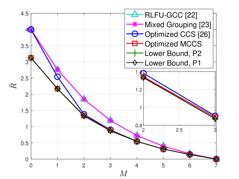
Let denote the average rate obtained by different schemes or the lower bound. Fig. 2 shows the average rate vs. for and . We generate the file popularities using the Zipf distribution with , where is the Zipf parameter. We set (used in [30, 49, 50]). We see that, among all the caching strategies, the optimized MCCS results in the lowest average rate for all values of . The two lower bounds in P1 and P2 are numerically identical, indicating the optimality of popularity-first placement. Comparing the optimized MCCS with the lower bounds, we see that the gap between them is very small and only appears at a small range of cache size values . The gap between the average rates of the optimized MCCS and the optimized CCS mainly exists for small cache size and shrinks as increases.
| Optimal cache placement vectors for the files | ||||||||
| CCS | 0 | 0 | 0 | 0 | 1.0000 | 1.0000 | 1.0000 | |
| 0.2500 | 0.2500 | 0.2500 | 0.2500 | 0 | 0 | 0 | ||
| 0 | 0 | 0 | 0 | 0 | 0 | 0 | ||
| 0 | 0 | 0 | 0 | 0 | 0 | 0 | ||
| 0 | 0 | 0 | 0 | 0 | 0 | 0 | ||
| MCCS | 0.4286 | 0.4286 | 0.4286 | 0.4286 | 0.4286 | 0.4286 | 0.4286 | |
| 0.1429 | 0.1429 | 0.1429 | 0.1429 | 0.1429 | 0.1429 | 0.1429 | ||
| 0 | 0 | 0 | 0 | 0 | 0 | 0 | ||
| 0 | 0 | 0 | 0 | 0 | 0 | 0 | ||
| 0 | 0 | 0 | 0 | 0 | 0 | 0 | ||
| Optimal cache placement vectors for the files | ||||||||
| CCS | 0 | 0 | 0 | 0 | 0 | 0 | 0 | |
| 0.2143 | 0.2143 | 0.2143 | 0.2143 | 0.2143 | 0.2143 | 0.2143 | ||
| 0.0238 | 0.0238 | 0.0238 | 0.0238 | 0.0238 | 0.0238 | 0.0238 | ||
| 0 | 0 | 0 | 0 | 0 | 0 | 0 | ||
| 0 | 0 | 0 | 0 | 0 | 0 | 0 | ||
| MCCS | 0 | 0 | 0 | 0 | 0 | 0 | 0 | |
| 0.2143 | 0.2143 | 0.2143 | 0.2143 | 0.2143 | 0.2143 | 0.2143 | ||
| 0.0238 | 0.0238 | 0.0238 | 0.0238 | 0.0238 | 0.0238 | 0.0238 | ||
| 0 | 0 | 0 | 0 | 0 | 0 | 0 | ||
| 0 | 0 | 0 | 0 | 0 | 0 | 0 | ||
| Optimal cache placement vectors for the files | ||||||||
| CCS | 0 | 0 | 0 | 0 | 0 | 0 | 0 | |
| 0 | 0 | 0 | 0 | 0 | 0 | 0 | ||
| 0 | 0 | 0 | 0 | 0 | 0 | 0 | ||
| 0.4286 | 0.4286 | 0.4286 | 0.4286 | 0.4286 | 0.4286 | 0.4286 | ||
| 0.1429 | 0.1429 | 0.1429 | 0.1429 | 0.1429 | 0.1429 | 0.1429 | ||
| MCCS | 0 | 0 | 0 | 0 | 0 | 0 | 0 | |
| 0 | 0 | 0 | 0 | 0 | 0 | 0 | ||
| 0 | 0 | 0 | 0 | 0 | 0 | 0 | ||
| 0.4286 | 0.4286 | 0.4286 | 0.4286 | 0.4286 | 0.4286 | 0.4286 | ||
| 0.1429 | 0.1429 | 0.1429 | 0.1429 | 0.1429 | 0.1429 | 0.1429 | ||
As discussed in Section VI-B, although the candidate solutions of the optimal cache placement for the MCCS and the CCS are the same, the optimal placements may be different for the two schemes. To see this difference, for the same setting considered in Fig. 2, we show the optimal for the two schemes for in Tables III, III, and III, respectively, representing small, moderate, and large cache size. For a small cache size (), the optimal placements for the MCCS and the CCS in Table III are different. For the MCCS, all files have the identical placement, where each file is partitioned into subfiles of two sizes, with one stored at the server () and the rest in each user’s local cache. In contrast, for the CCS, files are solely stored at the server, and files are stored in each user’s local cache. This difference on the placement is the main cause of the performance gap between the MCCS and the CCS in Fig. 2. For moderate to large cache size (), Tables III and III show that the optimal cache placements are the same for the MCCS and the CCS. However, we see from Fig. 2 that for , there is a small observable gap between the average rates of the two schemes, with that of the MCCS being lower; and for , the average rates of the two are nearly identical. The explanation for this trend is that there exist more redundant messages for with the placement in Table III than those for with the placement in Table III. To elaborate more on this, note that for given demand , the number of redundant groups in cache subgroup is , which decreases with . They determine the number of redundant messages. The indices of the nonzero elements in are for , and for . As a result, for , there are only a very small number of redundant messages that are removed by the MCCS. Thus, the performance of the MCCS and the CCS are almost identical. Finally, the larger improvement of the MCCS over the CCS (and the MCCS almost attains the lower bounds) for indicates that, at a small cache size, coded caching is more sensitive to the cache placement to achieve the largest caching gain.
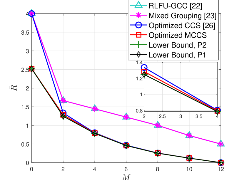
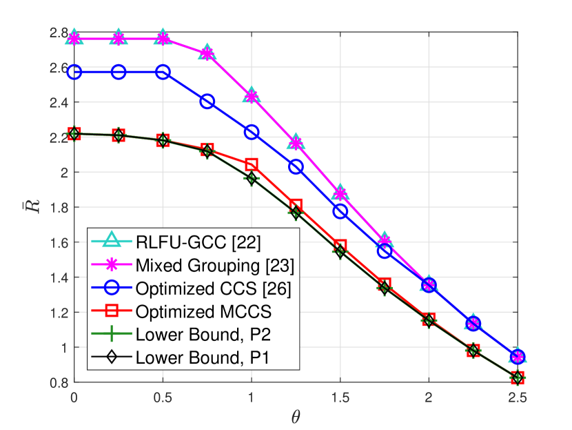
To evaluate the performance with other file popularity distribution, we consider the case studied in [23] with , , and a step-function for file popularity distribution: , , , and , . Fig. 4 shows the average rate vs. by different caching schemes and the lower bounds. Similar to Fig. 2, for all values of , the optimized MCCS achieves the lowest among all the strategies, which is very close to the lower bounds. The two lower bounds in P1 and P2 are equal for different values of , with the only exception for , where for P1 is smaller than that of P2. The gap between the MCCS and the CCS again only exists for small values of . To show the performance at different levels of popularity distribution, we show in Fig. 4 the average rate vs. Zipf parameter . We set , . We choose a small cache size to show clearly the performance gap between the caching schemes and lower bounds. The optimized MCCS always performs the best among all the caching strategies for any . The lower bound in P1 and the popularity-first-based lower bound in P2 are numerically identical. Also, we observe that the gap between the average rates of the optimized MCCS and the lower bounds only exists at a moderate range of and is very small in general. In contrast, the gap between the MCCS and the CCS is obvious at all values of . This demonstrates the advantage of the MCCS over other caching schemes at a small value of .
| Optimal cache placement vectors for the files | ||||||||||
| 0 | 0 | 0 | 0 | 1.000 | 1.000 | 1.000 | 1.000 | 1.000 | ||
| 0 | 0 | 0 | 0 | 0 | 0 | 0 | 0 | 0 | ||
| 0 | 0 | 0 | 0 | 0 | 0 | 0 | 0 | 0 | ||
| 0.250 | 0.250 | 0.250 | 0.250 | 0 | 0 | 0 | 0 | 0 | ||
| 0 | 0 | 0 | 0 | 0 | 0 | 0 | 0 | 0 | ||
| 0 | 0 | 0 | 0 | 0 | 0.667 | 1.000 | 1.000 | 1.000 | ||
| 0 | 0 | 0 | 0 | 0 | 0 | 0 | 0 | 0 | ||
| 0 | 0 | 0 | 0 | 0 | 0 | 0 | 0 | 0 | ||
| 0.250 | 0.250 | 0.250 | 0.250 | 0.250 | 0.083 | 0 | 0 | 0 | ||
| 0 | 0 | 0 | 0 | 0 | 0 | 0 | 0 | 0 | ||
| 0 | 0 | 0 | 0 | 0 | 0 | 0 | 0 | 0 | ||
| 0 | 0 | 0 | 0 | 0 | 0 | 0 | 0 | 0 | ||
| 0 | 0 | 0 | 0 | 0 | 0 | 0 | 0 | 0 | ||
| 0.222 | 0.222 | 0.222 | 0.222 | 0.222 | 0.222 | 0.222 | 0.222 | 0.222 | ||
| 0.111 | 0.111 | 0.111 | 0.111 | 0.111 | 0.111 | 0.111 | 0.111 | 0.111 | ||
We now verify the structure of the optimal cache placement for the MCCS described in Section VI-B. We generate file popularity using Zipf distribution with . We obtain the optimal placement solution using our proposed algorithm and verify that it matches the optimal solution obtained by solving P0 numerically. As an example, for and , Table IV shows the optimal that is obtained by solving P0 numerically, for . For , we see that there are two file groups and under the optimal placement. This structure matches Case 1 in Section 1, where the cache is entirely allocated to the first file group with the most popular files, and the files in the second file group are only stored at the server (). The optimal ’s for the first group are identical with only one nonzero element. This means those files are partitioned into subfiles of the same size and are stored at users’ local caches. With a small cache size, this placement result is intuitive: only a few popular files are cached, and the rest remain in the server; thus, the optimal cache placement results in two file groups. For , a different cache placement strategy is shown, where the files are divided into three file groups. The optimal is as described in Section VI-B3 for the three-file-group case: no cache is allocated to the third file group , and a portion of the file is cached for in the second file group; for the first file group, files are partitioned into subfiles of a single size and are all stored at different users. For , the optimal placement has only a single file group, where all the files have the same placement as discussed in Section VI-B1. From Table IV, we see that the file popularity differences are more critical for the placement when the case size is limited (relative to the total files in the database). As becomes large, all the files tend to have the same placement into the user caches.
Finally, we consider the scenario of nonuniform file popularity and size. We generate the file popularity using Zipf distribution with , which gives . The file sizes are set as kbits. The file size and popularity combinations are chosen similar to those used in [30], which simulate a practical scenario where file popularity and size are relatively uncorrelated. In Fig. 5, we compare the optimized MCCS in P4, the lower bound in P5, and the optimized CCS [30]. The gap between the optimized MCCS and the lower bound only exists for and is very small. Moreover, the optimized MCCS outperforms the optimized CCS. The gap between the two again is obvious at small values of , and it reduces to zero as becomes large.
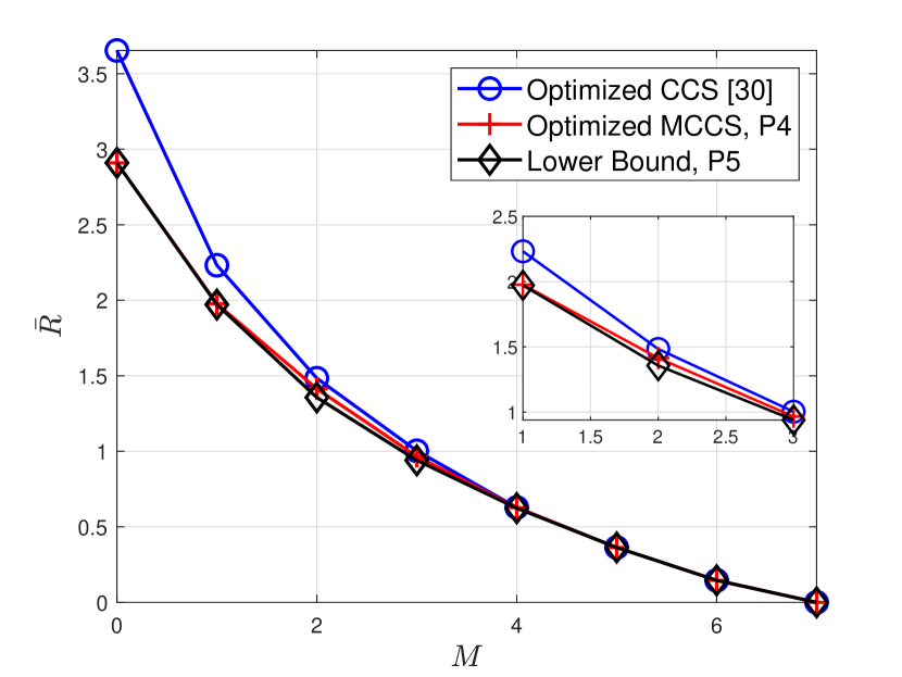
IX Conclusion
In this paper, for a caching system with nonuniform file popularity, we characterized the memory-rate tradeoff for caching with uncoded placement. We focused on the MCCS with cache placement optimized in the class of popularity-first placement for average rate minimization. We then provided a general lower bound and a popularity-first-based lower bound for caching with uncoded placement. For users, the two lower bounds are shown to be identical, and the optimized MCCS attains the bounds, providing the exact memory-rate tradeoff. For users with distinct requests, the optimized MCCS attains the popularity-first-based lower bound. Additionally, the results in these two regions reveal the following results for the MCCS unavailable in the literature: The popularity-first placement is optimal, and zero-padding used in coded delivery incurs no loss of optimality. For users with redundant requests, our analysis showed that a gap might exist between the optimized MCCS and the lower bounds due to zero-padding. However, numerical results show that such loss only exists in some limited cases and is very small in general.
We next characterized the optimal solution structure of the popularity-first cache placement for the MCCS under nonuniform file popularity. It was shown to have a simple file-grouping structure of at most three file groups, depending on the relative cache size to the database size. We obtained the closed-form placement solution for each candidate structure, which enabled us to compute the optimal solution through a simple algorithm. Finally, we extended our study of memory-rate tradeoff to the case where files are nonuniform in both popularity and size. We showed that the optimized MCCS attains the lower bound for users and characterizes the exact memory-rate tradeoff. Numerical results again showed that, for general settings, the gap between the optimized MCCS and the lower bound exists in limited cases and is very small.
Appendix A Proof of Lemma 1
Proof:
The proof directly follows the proof of [31, Theorem 2] with a slight modification. In the proof of [31, Theorem 2], by a genie-based method, it is shown that the delivery rate for a distinct file set satisfies
| (49) |
where is the total number of bits from file cached by exactly users. In our definition of , subscript refers to the user subset size in a cache subgroup , which is identical to that in . Following the definitions of and , we have , since there are user subsets in . Thus, for given , we can equivalently express (49) as
| (50) |
Using the above expression, by averaging over all possible , we obtain the general lower bound the average rate w.r.t in (11). The final lower bound on average rate is obtained by optimizing to minimize , which is shown in P1. ∎
Appendix B Proof of Lemma 2
Proof:
The popularity-first-based lower bound is essentially a simplification of P1 in Lemma 1, by restricting to the set of popularity-first placement vectors: . We need to show that in (12) can be simplified into (14) for . For , since is such that , by the definition of popularity-first placement in (4), for , we have
| (51) |
Since is a decreasing function of , for , we have
Thus, we remove the max operation in (12) to arrive at the simplified expression in (14), for . ∎
Appendix C Proof of Theorem 1
Proof:
For P1, consider a feasible cache placement vector and any . Define as a bijective map for such that . Note that depends on and .
Assume , for some . We construct another feasible cache placement
vector using by switching the values of and . Specifically,
i) for , we have
| (52) |
ii) for , by (52) and file partition constraint (2), we have
| (53) |
From (52), we have
| (54) |
For , we have
. Define as a bijective map for such that . Note that depends on . Then, in (12) is given by
| (58) |
Given , the set of distinct file indices in demand vector can be categorized into the following four types:
-
1.
, for .888Set corresponds to the case where file is requested and is ranked the th in .
-
2.
, for .
-
3.
.
-
4.
.
Note that for any , its type is the same for and . To see this, consider , where . Assume . Then for , we have , and . For , from (54), we also have . Thus, for the mapping for , we have , and in this case, we again have . All other types of can be verified using the similar argument.
We now evaluate the differences between and , for .
Case 1: . We express in (C) based on the types of . If , then , and we have
| (60) |
or more compactly, we can express (60) as follows
| (61) |
where is an indicator defined by . Similarly, for any other types of , we can always rewrite in (C) as in (61) by replacing and with and , given as follows
| (62) |
where the second and fourth cases are only for .
Similar to in (62), we can rewrite in (C) as follows
| (63) |
Comparing (62) and (63), we note that the only difference is the case of , where , while by (54).
Based on (62)–(65), we now compute for different types of . For , we have
| (66) |
where is by (64) and is due to (52). Similarly, using (54)(55)(64) and (65), we obtain the following for all the other types of
or more compactly,
| (67) |
Substituting (C) into (C), we have
| (68) |
where and , and the last inequality is due to the assumption that and for .
Case 2: . From the third case in (52), we have
| (69) |
For , , (56) and (57) are respectively given by
| (70) | |||
| (71) |
We compare and for different types of ’s. For , it is straightforward to show that the expressions of and are the same as the those for Case 1 () in (62) and (63), respectively. Similar to Case 1, based on (62) (63) and (69) – (71), except for , we have
| (72) |
For , we rewrite (C) for both and as follows
| (73) |
By (55), the sum of the first two terms in (73) is the same for and . By (69), the third term in (73) is identical for and . Thus, we have
| (74) |
Following (68), we substitute (C) and (74) into (C) and obtain the following
| (75) |
where and are defined below (68) and the inequality is due to the assumption that and for .
From the above results, we conclude that , for any . This means that, if , we can always reduce by switching the values of and . It follows that at the optimality of P1, we have , , for any satisfying , i.e., the optimal is a popularity-first cache placement. Thus, P1 and P2 are equivalent. ∎
Appendix D Proof of Lemma 3
Proof:
We look at each inner term of in (20), for . For cache subgroup , first consider , where for any user subset , includes user . Based on the relation of mappings and discussed above (16), we have , which is the size of the coded message for any user subset . By (16), (19), and , we have
| (76) |
Denote as the number of users that request file but are not in leader group . We have . For (in which user subsets includes user but not ,. among the total of user subsets, there are user subsets that do not contain any user that requests file . The size of coded messages corresponding to these user subsets is . For the rest of user subsets, since they contain at least one user from the redundant group that requests file , the size of coded message is . Thus, the size of coded message for user subset can be one of the above two cases, and we have
| (77) |
Following the similar arguments above, the size of coded message for user subset (i.e., including but not ,) can be one of the three types , and . It follows that
| (78) |
The first term in the above expression corresponds to the coded messages for the user subsets that contain users from the redundant group requesting file . The second term is for the coded messages for the user subsets that contain users from the redundant group requesting file but not . The third term represents the coded messages for all the rest user subsets in that do not request either file or .
Following the derivations above, we can obtain the general expression of with a recursive pattern. Let be the total number of redundant requests for files (i.e., file requests by users in the redundant group). We have . Similar to (76)–(D), for the coded messages for , we have
| (79) |
for . Assume that . From (76) – (D), we have
| (80) |
Appendix E Proof of Theorem 5
Proof:
To show that P4 and P5 are equivalent for , we will show that , for any given . To do so, we only need to compare and . For , we have or . We consider the two cases separately below.
E-1 For
E-2 For
Since two users request different files, we have the leader group . For , in (7) is given by
| (83) |
By the definition of , we have . Thus, we conclude that , and P4 and P5 are equivalent . ∎
References
- [1] Y. Deng and M. Dong, “Memory-rate tradeoff for caching with uncoded placement under nonuniform file popularity,” in Proc. 54th Asilomar Conf. on Signals, Syst., and Comput., 2020, pp. 336–340.
- [2] ——, “Optimal uncoded placement and file grouping structure for improved coded caching under nonuniform popularity,” in Proc. 18th Int. Symp. Modeling Opt. Mobile, Ad Hoc, Wireless Netw. (WiOPT), 2020, pp. 1–8.
- [3] E. Bastug, M. Bennis, and M. Debbah, “Living on the edge: The role of proactive caching in 5G wireless networks,” IEEE Commun. Mag., vol. 52, pp. 82–89, aug 2014.
- [4] X. Wang, M. Chen, T. Taleb, A. Ksentini, and V. Leung, “Cache in the air: exploiting content caching and delivery techniques for 5G systems,” IEEE Commun. Mag., vol. 52, pp. 131–139, Feb. 2014.
- [5] G. S. Paschos, G. Iosifidis, M. Tao, D. Towsley, and G. Caire, “The role of caching in future communication systems and networks,” IEEE J. Sel. Areas Commun., vol. 36, pp. 1111–1125, Sep. 2018.
- [6] M. A. Maddah-Ali and U. Niesen, “Fundamental limits of caching,” IEEE Trans. Inform. Theory, vol. 60, pp. 2856–2867, Mar. 2014.
- [7] ——, “Decentralized coded caching attains order-optimal memory-rate tradeoff,” IEEE/ACM Trans. Netw., vol. 23, pp. 1029–1040, Aug. 2015.
- [8] S. P. Shariatpanahi, S. A. Motahari, and B. H. Khalaj, “Multi-server coded caching,” IEEE Trans. Inform. Theory, vol. 62, pp. 7253–7271, Dec. 2016.
- [9] A. Sengupta, R. Tandon, and O. Simeone, “Fog-aided wireless networks for content delivery: Fundamental latency tradeoffs,” IEEE Trans. Inform. Theory, vol. 63, pp. 6650–6678, Aug. 2017.
- [10] M. A. Maddah-Ali and U. Niesen, “Cache-aided interference channels,” in Proc. IEEE Int. Symp. on Infor. Theory (ISIT), Jun. 2015, pp. 809–813.
- [11] M. Ji, G. Caire, and A. F. Molisch, “Fundamental limits of caching in wireless D2D networks,” IEEE Trans. Inform. Theory, vol. 62, pp. 849–869, Feb. 2016.
- [12] N. Naderializadeh, M. A. Maddah-Ali, and A. S. Avestimehr, “Fundamental limits of cache-aided interference management,” IEEE Trans. Inform. Theory, vol. 63, pp. 3092–3107, May 2017.
- [13] F. Xu, M. Tao, and K. Liu, “Fundamental tradeoff between storage and latency in cache-aided wireless interference networks,” IEEE Trans. Inform. Theory, vol. 63, pp. 7464–7491, Jun. 2017.
- [14] N. Karamchandani, U. Niesen, M. A. Maddah-Ali, and S. N. Diggavi, “Hierarchical coded caching,” IEEE Trans. Inform. Theory, vol. 62, pp. 3212–3229, Jun. 2016.
- [15] R. Pedarsani, M. A. Maddah-Ali, and U. Niesen, “Online coded caching,” IEEE/ACM Trans. Netw., vol. 24, pp. 836–845, Apr. 2016.
- [16] Q. Yu, M. A. Maddah-Ali, and A. S. Avestimehr, “The exact rate-memory tradeoff for caching with uncoded prefetching,” IEEE Trans. Inform. Theory, vol. 64, pp. 1281–1296, Feb. 2018.
- [17] Ç. Yapar, K. Wan, R. F. Schaefer, and G. Caire, “On the optimality of D2D coded caching with uncoded cache placement and one-shot delivery,” IEEE Trans. Commun., vol. 67, pp. 8179–8192, Dec. 2019.
- [18] K. Wan, D. Tuninetti, and P. Piantanida, “On caching with more users than files,” in Proc. IEEE Int. Symp. on Infor. Theory (ISIT), Jul. 2016.
- [19] ——, “On the optimality of uncoded cache placement,” in IEEE Infor. Theory Workshop, Sep. 2016.
- [20] U. Niesen and M. A. Maddah-Ali, “Coded caching with nonuniform demands,” IEEE Trans. Inform. Theory, vol. 63, pp. 1146–1158, Dec. 2017.
- [21] J. Hachem, N. Karamchandani, and S. N. Diggavi, “Coded caching for multi-level popularity and access,” IEEE Trans. Inform. Theory, vol. 63, pp. 3108–3141, Mar. 2017.
- [22] M. Ji, A. M. Tulino, J. Llorca, and G. Caire, “Order-optimal rate of caching and coded multicasting with random demands,” IEEE Trans. Inform. Theory, vol. 63, pp. 3923–3949, Apr. 2017.
- [23] J. Zhang, X. Lin, and X. Wang, “Coded caching under arbitrary popularity distributions,” IEEE Trans. Inform. Theory, vol. 64, pp. 349–366, Nov. 2018.
- [24] S. Jin, Y. Cui, H. Liu, and G. Caire, “Structural properties of uncoded placement optimization for coded delivery,” arXiv preprint arXiv:1707.07146, Jul. 2017.
- [25] S. A. Saberali, L. Lampe, and I. F. Blake, “Full characterization of optimal uncoded placement for the structured clique cover delivery of nonuniform demands,” IEEE Trans. Inform. Theory, vol. 66, pp. 633–648, Jan. 2020.
- [26] Y. Deng and M. Dong, “Fundamental structure of optimal cache placement for coded caching with nonuniform demands,” IEEE Trans. Inform. Theory, May 2022, doi: 10.1109/TIT.2022.3179266.
- [27] H. Cheng, C. Li, H. Xiong, and P. Frossard, “Optimal decentralized coded caching for heterogeneous files,” in the 25th European Signal Processing Conf., 2017.
- [28] J. Zhang, X. Lin, C. Wang, and X. Wang, “Coded caching for files with distinct file sizes,” in Proc. IEEE Int. Symp. on Infor. Theory (ISIT), 2015.
- [29] J. Zhang, X. Lin, and C. Wang, “Closing the gap for coded caching with distinct file sizes,” in Proc. IEEE Int. Symp. on Infor. Theory (ISIT), 2019.
- [30] A. M. Daniel and W. Yu, “Optimization of heterogeneous coded caching,” IEEE Trans. Inform. Theory, vol. 66, pp. 1893–1919, Mar. 2020.
- [31] S. Sahraei, P. Quinton, and M. Gastpar, “The optimal memory-rate trade-off for the non-uniform centralized caching problem with two files under uncoded placement,” IEEE Trans. Inform. Theory, vol. 65, pp. 7756–7770, Dec. 2019.
- [32] S. Jin, Y. Cui, H. Liu, and G. Caire, “Uncoded placement optimization for coded delivery,” arXiv preprint arXiv:1709.06462, Jul. 2018.
- [33] Q. Yu, M. A. Maddah-Ali, and A. S. Avestimehr, “Characterizing the rate-memory tradeoff in cache networks within a factor of 2,” IEEE Trans. Inform. Theory, vol. 65, pp. 647–663, Jan. 2019.
- [34] C. Chang and C. Wang, “Coded caching with full heterogeneity: Exact capacity of the two-user/two-file case,” in Proc. IEEE Int. Symp. on Infor. Theory (ISIT), 2019.
- [35] ——, “Coded caching with heterogeneous file demand sets — the insufficiency of selfish coded caching,” in Proc. IEEE Int. Symp. on Infor. Theory (ISIT), 2019.
- [36] S. Wang and B. Peleato, “Coded caching with heterogeneous user profiles,” in Proc. IEEE Int. Symp. on Infor. Theory (ISIT), 2019.
- [37] C. Chang, C. Wang, and B. Peleato, “On coded caching for two users with overlapping demand sets,” in Proc. IEEE Int. Conf. Communications (ICC), 2020.
- [38] C. Zhang and B. Peleato, “On the average rate for coded caching with heterogeneous user profiles,” in Proc. IEEE Int. Conf. Communications (ICC), 2020.
- [39] D. Cao, D. Zhang, P. Chen, N. Liu, W. Kang, and D. Gündüz, “Coded caching with asymmetric cache sizes and link qualities: The two-user case,” IEEE Trans. Commun., vol. 67, pp. 6112–6126, Sep. 2019.
- [40] A. M. Ibrahim, A. A. Zewail, and A. Yener, “Coded caching for heterogeneous systems: An optimization perspective,” IEEE Trans. Commun., vol. 67, pp. 5321–5335, Aug. 2019.
- [41] P. Hassanzadeh, A. M. Tulino, J. Llorca, and E. Erkip, “Rate-memory trade-off for caching and delivery of correlated sources,” IEEE Trans. Inform. Theory, vol. 66, pp. 2219–2251, Apr. 2020.
- [42] Q. Wang, Y. Cui, S. Jin, J. Zou, C. Li, and H. Xiong, “Optimization-based decentralized coded caching for files and caches with arbitrary sizes,” IEEE Trans. Commun., vol. 68, pp. 2090–2105, Apr. 2020.
- [43] Q. Yang and D. Gündüz, “Coded caching and content delivery with heterogeneous distortion requirements,” IEEE Trans. Inform. Theory, vol. 64, pp. 4347–4364, Jun. 2018.
- [44] P. Hassanzadeh, A. M. Tulino, J. Llorca, and E. Erkip, “Rate-distortion-memory trade-offs in heterogeneous caching networks,” IEEE Trans. Wireless Commun., vol. 19, pp. 3019–3033, May 2020.
- [45] E. Parrinello, A. Ünsal, and P. Elia, “Fundamental limits of coded caching with multiple antennas, shared caches and uncoded prefetching,” IEEE Trans. Inform. Theory, vol. 66, pp. 2252–2268, Apr. 2020.
- [46] Y. Deng and M. Dong, “Optimal cache placement for modified coded caching with arbitrary cache size,” in Proc. IEEE Int. Workshop on Signal Processing advances in Wireless Commun.(SPAWC), Jul. 2019.
- [47] U. Niesen and M. A. Maddah-Ali, “Coded caching for delay-sensitive content,” in Proc. IEEE Int. Conf. Communications (ICC), 2015.
- [48] S. Park, O. Simeone, and S. Shamai Shitz, “Joint optimization of cloud and edge processing for fog radio access networks,” IEEE Trans. Wireless Commun., vol. 15, pp. 7621–7632, Nov. 2016.
- [49] K. Shanmugam, N. Golrezaei, A. G. Dimakis, A. F. Molisch, and G. Caire, “Femtocaching: Wireless content delivery through distributed caching helpers,” IEEE Trans. Inform. Theory, vol. 59, pp. 8402–8413, Dec. 2013.
- [50] M. Zink, K. Suh, Y. Gu, and J. Kurose, “Characteristics of youtube network traffic at a campus network–measurements, models, and implications,” Comput. Netw., vol. 53, pp. 501–514, Apr. 2009.