Intelligent Reflecting Surface Enabled Random Rotations Scheme for the MISO Broadcast Channel
Abstract
The current literature on intelligent reflecting surface (IRS) focuses on optimizing the IRS phase shifts to yield coherent beamforming gains, under the assumption of perfect channel state information (CSI) of individual IRS-assisted links, which is highly impractical. This work, instead, considers the random rotations scheme at the IRS in which the reflecting elements only employ random phase rotations without requiring any CSI. The only CSI then needed is at the base station (BS) of the overall channel to implement the beamforming transmission scheme. Under this framework, we derive the sum-rate scaling laws in the large number of users regime for the IRS-assisted multiple-input single-output (MISO) broadcast channel, with optimal dirty paper coding (DPC) scheme and the lower-complexity random beamforming (RBF) and deterministic beamforming (DBF) schemes at the BS. The random rotations scheme increases the sum-rate by exploiting multi-user diversity, but also compromises the gain to some extent due to correlation. Finally, energy efficiency maximization problems in terms of the number of BS antennas, IRS elements and transmit power are solved using the derived scaling laws. Simulation results show the proposed scheme to improve the sum-rate, with performance becoming close to that under coherent beamforming for a large number of users.
Index Terms:
Intelligent reflecting surface (IRS), multiple-input single-output (MISO) broadcast channel (BC), multi-user (MU) diversity, average sum-capacity, sum average rate, energy efficiency (EE).I Introduction
Although the emerging Fifth-Generation (5G) era has brought about a remarkable improvement in the speed, latency and reliability of cellular networks, it still faces challenges related to the high power consumption of the underlying technologies as well as the limited control over the wireless propagation environment [1]. A promising new solution to address these issues is deploying intelligent reflecting surfaces (IRSs) [2, 3, 4, 5] in existing wireless communication systems. The IRS is abstracted in the current literature as an array of nearly passive reflecting elements, where each element can introduce a phase shift onto the incoming electromagnetic waves as directed by a smart controller [3, 4, 2, 5, 6, 7, 8, 9, 10]. The resulting software-controlled reflections can tailor the propagation environment to yield desirable communication objectives, like increase the coverage, rates, energy efficiency etc, in a passive manner without generating new radio signals.
Motivated by its numerous potential advantages, IRS-assisted communication has recently been investigated under different communication scenarios [7, 5, 8, 6, 9, 10]. Several joint designs for precoding at the base station (BS) and reflect beamforming at the IRS have been proposed to achieve different communication goals, for example: maximize the system’s energy efficiency subject to signal-to-interference-plus-noise ratio (SINR) constraints at the users in [7], maximize the minimum user rate subject to a transmit (Tx) power constraint at the BS in [8], minimize the Tx power subject to users’ SINR constraints in [5], maximize the sum-rate subject to a Tx power constraint in [9], and minimize the Tx power subject to a secrecy rate constraint in [10].
All these works optimize the IRS phase-shifts assuming the availability of perfect channel state information (CSI) at the BS and IRS of the individual IRS-assisted links, that is the BS-IRS link and IRS-users links. However, reliable channel estimation of these individual links in IRS-assisted systems can cause a prohibitive training overhead due to the inability of the IRS to send, receive or process the pilots. The preliminary papers on channel estimation for these systems showed the required training time to estimate the individual IRS-assisted channels to grow proportionally with the number of IRS elements [11, 12, 13, 14], thus compromising the performance gains expected from deploying a large number of reflecting elements to a large extent. Moreover, optimizing the IRS phase-shifts at the pace of fast-fading channel significantly increases the system complexity.
Motivated by these challenges, this paper presents an information-theoretic analysis of an IRS enabled random rotations scheme in the multiple-input single-output (MISO) broadcast channel (BC). The proposed scheme requires the IRS elements to only introduce random phase rotations in each coherence interval without requiring instantaneous CSI. The BS will only require the CSI of the overall BS-users channels (or SINRs), instead of the individual IRS-assisted channels, to implement the precoding/beamforming scheme. The only other works that have analytically studied the random rotations scheme at the IRS are [15] and [16], where the former develops low-complexity and energy-efficient transmission schemes for a point-to-point IRS-assisted single-input single-output (SISO) system based on coding and selection approaches, while the latter studies the sum-rate of the SISO BC under opportunistic scheduling.
We define the MISO BC from an information-theoretic point-of-view as consisting of a single multi-antenna transmitter (or BS) communicating with multiple single-antenna users, where the BS transmits different data signals (intended for different users) from different transmitting antennas [17, 18, 19, 20, 21]. For the MISO BC, the primary research focus has been on 1) quantifying the maximum achievable average sum-rate capacity, and 2) devising computationally efficient algorithms for capturing most of this capacity. The first question has been addressed using dirty paper coding (DPC) [22, 19], which solves the MISO BC problem optimally. The average sum-rate capacity (referred to as sum-capacity in this paper) achieved by DPC in a Gaussian BC is shown to scale as , with the number of users for a fixed number of Tx antennas [21, 18]. While the capacity increase is linear in , DPC is computationally expensive and requires full CSI, motivating the development of sub-optimal schemes that use partial CSI.
A popular scheme that addresses these challenges is random beamforming (RBF), which constructs random orthonormal beams and on each beam transmits to the user with the highest SINR. At the start of a coherence interval, each user measures downlink SINR values corresponding to the pilot symbols transmitted on the beams by the BS, and feeds back only one real number (its best SINR) and the corresponding beam index. The feedback overhead is therefore much less than sending back complex numbers associated with the full channel information required by DPC. The BS then schedules the best user to transmit to on each beam. Interestingly, the sum average rate scaling of RBF is shown to asymptotically coincide with the average sum-capacity scaling achieved by DPC, i.e. the sum average rate achieved by RBF also scales as [18]. The gain with is explained by the multi-user (MU)-diversity effect [23], i.e. in a system with many users with independently time-varying channels, it is very likely to have at each time some users whose SINRs are much higher than the average SINR and by scheduling these users, the sum-rate can be significantly increased. This MU-diversity effect can be enhanced by increasing the dynamic range of channel fluctuations. We propose to do this using the time-varying random rotations introduced by an IRS into the BS-users channels. Our idea is inspired from the rotate-and-forward protocol proposed in [24] for the slow-fading relay channel, where artificial fast fading created using the random rotations at the relay resulted in an optimal diversity-multiplexing tradeoff.
Motivated by these works, we consider incorporating an IRS into the conventional MISO BC, where the BS-IRS channel is line-of-sight (LoS), the IRS-users channels and BS-users direct channels are Rayleigh faded and the IRS elements induce only random phase rotations. The assumption that the BS-IRS channel is LoS dominated has also been made in many other works such as [6, 25, 26, 27, 28, 29, 8, 14, 13] and is quite practical given the BS and IRS have fixed positions with few obstacles around. The overriding question then is to study the effect of the IRS enabled random rotations scheme on the average sum-capacity scaling (achieved by DPC) and the sum average rate scaling achieved by RBF. We carry out an asymptotic study of the sum-rate in the limit of a large number of users, leveraging results from extreme value theory, and find that the random phase rotations at the IRS increase the MU-diversity gain. At the same time, the spatial correlation introduced in the overall channel by the BS-IRS LoS link reduces the sum-rate [20]. We study the interplay between the MU-diversity gain and the rate loss due to correlation in the developed scaling expressions. Under a deterministic variation of RBF, referred to as deterministic beamforming (DBF), the sum average rate scaling is shown to coincide with the average sum-capacity scaling. Simulation results show a significant sum-rate gain with the random rotations scheme. Interestingly, the performance gap between the proposed scheme and coherent beamforming (under which the IRS phase shifts are designed based on full CSI) is shown to significantly reduce for large .
We also optimize the system in terms of energy efficiency (EE) by obtaining the optimal system configuration parameters, including the number of BS antennas, the number of IRS elements and the total Tx power, that maximize the EE. The developed sum average rate scaling expression for DBF along with a realistic power consumption model are used to formulate the EE scaling. The challenging problem, that involves two discrete variables appearing as upper limits of sums and products, is solved using alternating optimization and line search methods subject to constraints on the maximum values of the parameters. Simulation results show the EE performance of the IRS-assisted system to be significantly better than the conventional system.
The paper is organized as follows. In Sec. II, the MISO BC and IRS enabled random rotations scheme are outlined. In Sec. III, the average sum-capacity scaling law for DPC and the sum average rate scaling laws for RBF and DBF are derived. In Sec. IV we maximize the EE with respect to the number of BS antennas, IRS elements and Tx power. Simulation results and conclusions are provided in Sec. V and Sec. VI respectively.
II System Model
In this section, we outline the transmission model for the IRS-assisted MISO BC.
II-A MISO BC
Consider a Gaussian BC from an -antenna BS to single-antenna users under the block-fading model, where the channel is constant during a coherence interval of length time-slots and varies independently from one such interval to the next. Let be the vector of Tx symbols in time-slot , then the received signal, , at user in time-slot is given as
| (1) |
where is the channel from the BS to user and is the complex Gaussian noise with zero mean and variance . We assume that the average Tx power, denoted as , is fixed at at all times and therefore the Tx signal vector must satisfy the power constraint , . Denoting the average rate of user as , where the average is taken over the fading distribution of , we are interested in analyzing the behavior of the downlink sum average rate, i.e., .
II-B IRS-Assisted Channel Model
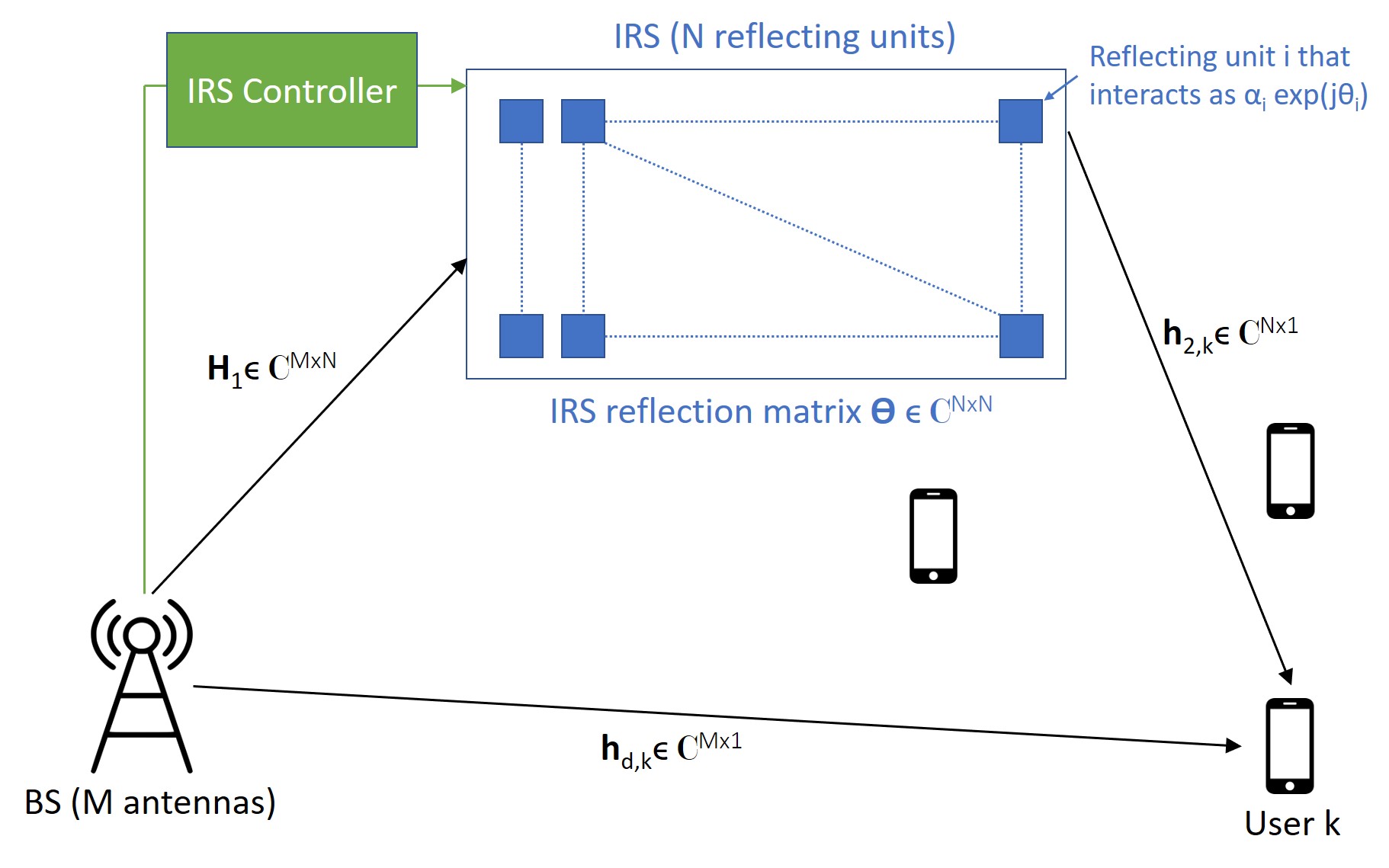
The communication from the BS to users is assisted by an IRS, composed of passive reflecting elements (See Fig. 1). The resulting channel between the BS and user is
| (2) |
where is the channel between the BS and the IRS, is the channel between the IRS and user , is the direct channel between the BS and user , and accounts for the IRS response. Here is the phase shift applied by element and is the reflection coefficient of element which is fixed and depends on the IRS construction. Under the random rotations scheme, each is randomly drawn from the uniform distribution over the interval , with a new set of phase-shifts applied in each coherence interval. Moreover , where , and are the path loss factors for BS-IRS, IRS-user- and direct links respectively.
The channel between the BS and IRS is considered to be LoS dominated. This assumption, made in many other related works [6, 25, 26, 27, 28, 29, 8, 14], is supported in literature using two points. First, the LoS path between the BS and the IRS will usually always exist. The BS tower is generally elevated high and the IRS is also envisioned to be integrated onto tall structures in the environment, so both will have a few obstacles around. Given the positions of BS and IRS are fixed, a stable LoS channel between the BS and the IRS is expected to exist and can be constructed using the directional angular information. Second, the path loss for NLoS paths is much larger than that for the LoS path in the next generation systems. In fact it is noted that in mmWave systems, the typical value of Rician factor (ratio of energy in LoS to that in NLoS component) is between dB and dB [25], which is sufficiently large to neglect any NLoS channel components in as compared to the LoS component. Under these remarks, we assume that the BS-IRS channel is LoS dominated and neglect any NLoS paths in this channel.
A uniform rectangular array (URA) of reflecting elements is considered at the IRS, where and are the number of elements placed with inter-element spacing and along the two principal directions of the URA, characterized by unit vectors and respectively. Here () are the LoS azimuth and elevation angles that describe these principal directions at the IRS. A uniform linear array (ULA) is considered at the BS, with antennas placed at a spacing of units along , described by the LoS angles (). Under the spherical wave model, the entries of the LoS channel are computed as [30]
| (3) | ||||
where , , and is the path length between the BS antenna and IRS element , given as . Here is the steering vector from the global origin (defined as first antenna in the BS ULA) to the IRS element , and is the steering vector from global origin to the BS antenna . The expressions of and can be found in [30, equations (12) and (13)] and depend on , , , the distance between the BS and IRS as well as the expressions of the unit vectors and provided in [30, equations (6) and (9)]. An important observation is that we have taken the spherical nature of the electromagnetic wave propagation into account, by applying the actual distance between the Tx antennas and receive (Rx) elements when considering the received LoS phase in (3). Consequently, there is no restriction on the rank of , which can generally be of high rank for moderate BS-IRS distances and large [30].
Also, we consider the IRS-users channels ’s and BS-users direct channels ’s to undergo Rayleigh fading. This is justified by observing that the LoS paths in these channels are usually blocked due to the scattering and blocking structures/objects around the ground users. These links are therefore characterized by NLoS paths and are modeled as and , with the channels being independent across the users. The overall channel in (2) is a sum of two zero-mean complex Gaussian vectors, where the second vector (i.e. ) has uncorrelated elements. The first vector has correlated entries with the correlation matrix found by conditioning the expectation on first as . Therefore, the overall channel in (2) under the random rotations scheme is distributed as
| (4) |
where is the covariance matrix of the overall channel. It can be written using (3) as
| (5) |
III Asymptotic Analysis of the Sum-Rate
We now study the scaling laws of the average sum-capacity (achieved by DPC) and the sum average rate achieved by RBF and DBF against the number of users , under the proposed framework using the following result from extreme value theory.
Lemma 1
[23, Lemma 2]: Let be independent and identically distributed (i.i.d.) random variables (RVs) with a common cdf and pdf , satisfying for all finite and is twice differentiable for all . The distributions are such that they satisfy
| (6) |
for some constant , where . Then for satisfying , we have
| (7) |
converges in distribution to a limiting random variable with CDF .
This lemma states that the maximum of i.i.d. RVs described above grows like as .
To study the asymptotic behaviour of the sum-rate, we will assume a homogeneous network as done in many works including [18, 20, 21, 23, 31]. The assumption is stated below.
Assumption 1: We assume , , resulting in , .
Note that the users’ channels in (4) are independent by noting that for . Assumption 1 will ensure that they are identically distributed as well. This makes the analysis based on extreme value theory tools tractable since Lemma 1 is applicable to i.i.d. RVs.
III-A Average Sum-Capacity Scaling of the Proposed Framework
For the case where full CSI is available at the BS and users, it has been shown that the average sum-capacity of the Gaussian BC can be achieved using DPC. Intuitively, if the BS knows the channels ’s of all users, it can use DPC to code against the interference for each user while preserving the power constraint. The average sum-capacity is written as [18]
| (8) |
where is the optimal power allocation and the expectation is performed with respect to the distribution of ’s. In a system without IRS, is shown to scale for large as [18]
| (9) |
Here, we develop the average sum-capacity scaling law for the IRS-assisted MISO BC under the random rotations scheme. Intuitively, different from [18], the sum-capacity will be affected 1) positively by the IRS array gain as highlighted through the sum over in the diagonal elements of (5), and 2) adversely by the correlation in the IRS-assisted channel in (4). The proof of the scaling law (presented in the following theorem) starts by establishing an upper bound on the average sum-capacity scaling and showing that this bound is achievable using a low-complexity DBF scheme outlined in Sec. III-C.
Theorem 1
Consider the Gaussian BC given in (2) comprising of an -antenna BS serving single-antenna users. This communication is assisted by an -element IRS inducing only random phase rotations. Assume that the BS and users have perfect CSI of ’s. Let , and be fixed, then for large and under Assumption 1, the average sum-capacity scales as
| (10) |
where .
Proof:
The proof is provided in Appendix A. ∎
We observe that , with equality when is an identity matrix. This is because the sum of the eigenvalues of is since (Observe using (5) that all diagonal elements of will equal 1). Therefore, the product of these eigenvalues, which is , would be less than or equal to . As compared to the result in (9) for a MISO BC without IRS, the average sum-capacity is increased by and decreased by a constant , when an IRS introducing random phase rotations is incorporated into the system. However as increases, one can expect the positive effect of to dominate, resulting in significant performance gains by deploying an IRS in the MISO BC.
There are two major drawbacks of DPC. First, it is computationally very complex, both at the BS and users. Moreover, it requires full CSI feedback of the overall channel from each user to the BS resulting in prohibitively high feedback overhead when and are large. Therefore, research has focused on devising schemes that impose less computational complexity and feedback requirements but still achieve most of the sum-rate promised by DPC. The computational cost and feedback overhead associated with DPC are discussed in Sec. III-D.
Remark 1
When each user has receive antennas, the average sum-capacity (of DPC) scales as . The result can be proved using a similar extension as done in [21].
III-B Random Beamforming
To serve multiple users simultaneously without having full CSI at the BS, the RBF scheme was proposed in [18] that constructs random beams and on each beam transmits to the user with the highest SINR. The only feedback required from each user is its maximum SINR along with the beam index on which the SINR is maximized, instead of complex numbers representing the estimate of as required by DPC. The process of RBF is explained in detail below.
At the start of each coherence interval, the BS generates random orthonormal beamforming vectors of size for , according to an isotropic distribution. A straightforward way to generate the RBF matrix, , containing the isotropically distributed (i.d.) orthonormal beamforming vectors is outlined in [32]. The method entails that we first generate a random matrix whose elements are i.i.d. RVs and then perform its QR (Gram-Schmidt) factorization as , where is an i.d. unitary matrix and is an upper triangular matrix. This yields the RBF matrix as . The proof that is indeed i.d. with orthonormal vectors can be found in [32, Appendix A].
Then at time-slot , the BS multiplies the beamforming vector with the transmit data symbol denoted as , such that the transmitted signal vector is given as
| (11) |
In this paper, we assume the data symbols to be i.i.d. letters from codewords of a Gaussian capacity-achieving codebook with , where . The Tx signal vector then satisfies the power constraint . After the coherence interval of channel uses, the BS chooses another set of orthonormal vectors and constructs the signal in (11) and so on. From now on, we drop the time index for simplicity.
The RBF scheme allows users to be served simultaneously on the random beams (i.e. on the beamforming vectors ’s). These out of users are selected based on their SINR feedback. Specifically during the training phase at the start of a coherence interval, the BS transmits orthogonal pilot symbols on the random beams , . Denoting the pilot symbol transmitted on beam as , with the pilot symbols satisfying the same power constraint as data symbols, the received signal at user during the training phase is
| (12) |
User then computes the following SINRs by assuming that is the desired signal and the others are interfering signals:
| (13) |
Note that the SINRs above, corresponding to beams, are computed at the user by correlating the received signal in (12) one-by-one with each pilot symbol as . Given the orthogonality of pilot symbols, this allows the users to estimate corresponding to beams, and hence compute the ’s defined in (13). Also note that the beams are associated with pilot symbols. Therefore, the user uses the pilot symbols to know which beam (i.e. which ) it is processing and get the corresponding SINR for that beam.
Once the user has computed for beams, it feeds back its maximum SINR, i.e. , along with the beam index (i.e. the index of ) on which the SINR is maximized. Once the BS has this partial CSI from all users, it assigns the beamforming vector to transmit data symbol to the user with the highest corresponding SINR, i.e. on beamforming vector serve the user . Using this scheduling, the BS constructs the signal vector in (11). The sum average rate during downlink transmission can then be written as [18]111More rigorously the maximization in (14) over should be performed over the subset (or fraction ) of users who report as the maximizing beam index. In practice, the users will not report beam index when either this was not the beam on which they observed the maximum SINR or they did not receive that beam (due to channel being orthogonal to ). However as grows large, the impact of this fraction on the average rate scaling achieved on each beam will grow to zero because as , which is why the definition in (14) with term added is utilized [18, 20, 31, 21].
| (14) |
where is given by (13) and represents the terms that go to zero as .
Note that if user has maximum SINR on two beams then the BS has to schedule another (weaker) user on one of these two beams resulting in a decrease in the sum average rate. However, it is shown in [18] that the probability that user has maximum SINR on two beams goes to zero as grows large, and therefore the sum average rate is given by (14) with added to represent the terms that go to zero with .
The authors in [18] studied the behaviour of (14) for a MISO Gaussian BC without an IRS, where , and showed the resulting scaling law with to be given as
| (15) |
In this section, we will investigate the impact of the random rotations IRS scheme on this scaling law. In [18], the sum average rate does not depend on the distribution of ’s as multiplying the circularly symmetric complex Gaussian vector with a unitary vector does not change its distribution. However for our correlated scenario, the expectation in (14) depends on both the distribution of ’s and the distribution of ’s and is written as
| (16) |
i.e., we first condition on and calculate the expectation over ’s and subsequently take the expectation over . The distribution of given (stated below) is calculated using an approach similar to the one in [20], which studied the correlated Gaussian BC.
Lemma 2
Using the derived CDF and PDF of SINR, we develop the scaling law of given . Since are i.i.d. across (for a given ) due to the channels being i.i.d. across as discussed after Assumption 1, so the only condition remaining to be checked to apply Lemma 1 on (III-B) is whether the growth function satisfies (6). For this, we require the following result.
Lemma 3
The maximum eigenvalue of , denoted as , and the corresponding eigenvector are given by
| (19) |
Proof:
The proof is provided in Appendix B. ∎
Note that although is a function of , its maximum eigenvalue and corresponding eigenvector are not. Using this result, we can verify the condition in (6) as follows.
Proof:
The proof follows from using (17) and (18) to obtain
It is obvious from the definition of in Lemma 2 that for (we showed that is independent of in Lemma 3). Therefore and . Using the definition of and from Lemma 3 and that of from Lemma 2, we can obtain . The only non-zero term is which is simplified to obtain the result. ∎
Lemma 4 therefore implies that converges in distribution to a limiting RV, where can be found using Lemma 1. The resulting scaling law is stated below.
Theorem 2
Consider the Gaussian BC in (2) comprising of a BS with antennas, an IRS with elements and single-antenna users. Then under Assumption 1, with RBF at the BS and random uniform phase allocation at the IRS, the sum average rate scales as
for large , where .
Proof:
The proof can be found in Appendix C. ∎
Remark 2
The implementation of the scenario described in Theorem 2 is as follows. At the start of each coherence interval, the -antenna BS generates random orthonormal i.d. beamforming vectors , according to the Gram-Schmidt decomposition method described at the start of Sec. III-B, while the IRS applies a set of phase shifts , across the reflecting elements, which are drawn from the uniform distribution over . The IRS continues to apply the same set of phase shifts during the training phase and the downlink transmission phase of the coherence interval. During the training phase, the BS transmits pilot symbols on the random beams (i.e. on ’s) and each user measures the downlink SINRs defined in (13). Each user then feeds back its maximum SINR i.e. , along with the beam index on which the SINR is maximized. Once the BS has this partial CSI, it assigns the beamforming vector to transmit data symbols to the user with the highest corresponding SINR, i.e. on beamforming vector transmit to user . Using this scheduling, the BS constructs the signal vector in (11) and starts data transmission. After the coherence interval of channel uses, the BS chooses another set of beamforming vectors ’s and IRS applies another set of uniformly drawn random phase shifts and the process is repeated. The sum average rate scaling for this framework is provided in Theorem 2.
To complete the result in Theorem 2, it remains to calculate the expectation . The final scaling law after evaluating this expectation is given in Theorem 3 below.
Theorem 3
Under the setting of Theorem 2, the sum average rate scaling of RBF is given as
| (21) |
where , is the diagonal element of and .
Proof:
The expression is involved but yields some insights. There is an increase in the sum average rate as compared to (15) by a factor of . However, there is also a decrease corresponding to , due to the correlated nature of the channel.
Remark 3
The analysis can be extended to the scenario with antennas at each user. A direct extension is to treat each receive antenna as an independent user and have effectively single antenna users [18]. Therefore, each user will feed back times the amount of information because corresponding to each receive antenna , the user needs to feed back the maximum SINR, i.e. along with the maximizing beam index . The BS then assigns beamforming vector , to transmit data symbols to the antenna of the user with the highest SINR, i.e., . Since the maximization is over i.i.d. RVs, the scaling law will be the same as the one in Theorem 3 with replaced by .
The results can be extended, using some involved analysis, to the case where at most one beam is assigned to each user by computing the overall SINR of each user instead of the SINR for each receive antenna separately. However, this is beyond the scope of this work.
III-C Deterministic Beamforming
We also study the case where the matrix is fixed over all channel uses and refer to this scheme as DBF [20]. The analysis stays the same as that for RBF, except that we do not need to take the expectation over in Theorem 2. The sum average rate is then written as
| (22) |
for large , where and is the eigenvalue decomposition of . An interesting special case will be when are columns of the identity matrix. In this case, the DBF matrix is equal to and therefore . This leads to . Thus we obtain the following result.
Theorem 4
Consider the Gaussian BC in (2) comprising of a BS with antennas, an IRS with elements and single-antenna users. Then under Assumption 1, the DBF scheme at the BS and random phase rotations at the IRS, the sum average rate scales as
| (23) |
As compared to the sum average rate scaling in the conventional MISO BC given by (15), we see that the random-rotations IRS scheme increases the sum-rate by and decreases it by since . This also proves that the right hand side of the upper bound on the average sum-capacity scaling in (A) is achievable, and thus (4) acts as a lower bound to the average sum-capacity scaling and completes the proof of Theorem 1.
III-D Complexity and CSI Overhead Comparison
So far we have developed the scaling laws of the average sum-capacity and the sum average rate for different transmission schemes at the BS while employing the random rotations scheme at the IRS. The main motivation behind using the random rotations scheme at the IRS is as follows. Unlike the coherent beamforming scheme where the IRS phase shifts need to be optimized based on the instantaneous CSI of IRS-user () and BS-user () channels, the proposed scheme does not require the availability of the instantaneous CSI of these individual IRS-assisted and direct channels to implement the random phase shifts. The only CSI needed is, therefore, at the BS of the overall channel to implement the beamforming transmission scheme. This saves the large training overhead associated with the estimation of ’s and ’s [14]. Also, the random rotations scheme reduces the system complexity since optimizing IRS-phase shifts at the pace of fast-fading channels is not required.
In this part, we discuss the computational complexity and CSI feedback overhead associated with the beamforming schemes considered at the BS. The sum-capacity of a Gaussian BC is achieved by DPC [22], based on the idea that when the interference caused by other users’ signals is known at the BS in advance (non-causally), it is possible to achieve the same capacity as if there was no interference by successively encoding the users while preserving the power constraint. DPC is well-known to be extremely computationally intensive to implement due to the high computational burden of successive encoding and decoding [33]. The exact complexity in terms of the number of complex arithmetic operations largely depends on the implementation of the DPC based optimal algorithm. An efficient iterative algorithm was proposed by Jindal et al in [34], which requires operations per iteration. To circumvent this problem, many works advocate the use of the linear zero-forcing (ZF) beamforming to create orthogonal channels between the BS and users. Since in our setting, , so we consider ZF with user selection (ZFS) from [33] as a benchmark scheme in the simulations, wherein the user selection procedure has a computational complexity of while ZF with selected users has a complexity of [35]. Both DPC based algorithms and ZF require full CSI feedback from all users to the BS. Therefore, each user needs to feedback real numbers corresponding to to the BS at the start of each coherence interval.
We then studied two low-complexity beamforming schemes that require partial CSI at the BS. Both RBF and DBF require each user to feedback only one real number (its maximum SINR) and the corresponding beam index (an integer) to the BS at the start of each coherence interval, which is significantly less than the CSI overhead associated with DPC-based and ZF schemes. In terms of implementation, RBF requires random orthonormal beams ’s to be generated according to an isotropic distribution, which has a computational complexity of per coherence interval. DBF requires the beamforming matrix to be set as obtained from the eigenvalue decomposition of , which also has a computational complexity of . However this computation does not need to be performed per coherence interval but only when the large-scale channel statistics change after several coherence intervals. The user selection algorithm (i.e. finding the user with maximum SINR on each beam) at the BS for both RBF and DBF has a computational complexity of , which is significantly less than that of ZFS.
Overall, both RBF and DBF impose a significantly lower CSI feedback overhead than DPC and ZFS. The associated user scheduling scheme for RBF and DBF also has a reduced complexity. These observations are summarized in Table I, along with the computational complexity and CSI feedback results for the random rotations IRS scheme and the benchmark coherent IRS beamforming scheme (implemented in simulations using exhaustive search with phase shift levels).
| Scheme | Feedback | Complexity of Beamforming | Complexity of User |
| (in real numbers) | (for selected users) | Selection | |
| Base Station | |||
| ZFS [33] | |||
| RBF | [18] | ||
| DBF | [18] | ||
| IRS | |||
| Random rotations | None | - | |
| Coherent BF | - |
IV Energy Efficiency Optimization
In this section, we optimize the IRS-assisted MISO BC in terms of EE by using the sum-rate results developed in last section. Current works that study the EE of IRS-assisted MISO BC consider coherent beamforming schemes at the IRS under perfect CSI assumption. Different from these works, we consider the random rotations scheme at the IRS and DBF (or RBF) at the BS. Under this framework, no CSI is needed at the IRS since it just introduces random phase-shifts from the uniform distribution and only partial CSI is needed at the BS to implement DBF or RBF. Under this setting, we aim to obtain the optimal system configuration parameters, including the numbers of BS antennas and IRS elements and the Tx power , that maximize EE. The main analysis is presented for DBF at the BS and extends straightforwardly to RBF as well.
IV-A Problem Formulation
We first describe the power consumption model, which will consist of the Tx power at the BS, the circuit power consumed at the BS and users, the static power consumed at the BS and the power consumed at the IRS. The total power consumed is given as
| (24) |
where is the power amplifier efficiency. The circuit power model is given as [36]
| (25) |
where , , , , and represent the power consumed in the mixer, filters of transmitter and receiver, low noise amplifier, digital-to-analog converter (DAC) and analog-to-digital converter (ADC), respectively. The IRS power consumption is given as , where is the power consumed by one IRS element and is the static power consumption of the IRS. The total power can then be written in a compact form as
| (26) |
where , , , , and .
Since the focus of this work is on the large regime, we utilize the sum average rate scaling expression derived in (4) to formulate the EE scaling expression under DBF as
| (29) |
where .
To determine the optimal values of the number of BS antennas , the number of IRS elements , and the optimal power , we consider the following problem:
| (32) |
subject to constraints on the maximum number of deployable transmit antennas and IRS reflecting elements, i.e. and , and on the maximum feasible Tx power, i.e. .
To explicitly show the dependence of on and , we express the determinant of using Leibniz formula and the definition of in (3) to obtain
| (35) |
where represents the set of all permutations of , where each permutation denoted as is the column of . Moreover denotes the signature of which will be if is an even permutation and if is an odd permutation.
Finding the optimal solution of (32) with affordable complexity is complicated due to the fact that two of the three variables are discrete and also that both and appear as the upper limits of sums and products terms as seen in (35), which prevents us from using standard gradient-based methods. For these reasons, we will consider both the maximization of the exact objective of (32) by line searches methods, and the maximization of a bound of this objective.
IV-B Exact Solution of Problem (P1)
The global solution of Problem (P1) can be determined by an exhaustive search in the set . Using a step size to search the continuous set , this approach requires computations and comparisons of the values of the objective function of (32). Although globally optimal, this technique might be too demanding for large values of and , or for low values of .
A first approach to reduce the computational complexity is based on the use of alternating maximization to optimize (32) with respect to , , and one variable at a time, while keeping the other two fixed. Formally, denoting by the objective of Problem (P1), an alternating maximization algorithm for Problem (P1) can be stated in Algorithm 1.
The convergence of Algorithm 1 is ensured by the fact that at each step the objective function does not decrease. Since EE can not grow to infinity, Algorithm 1 must eventually converge in the value of the objective. As for its complexity, Algorithm 1 requires two exhaustive searches in each iteration to optimize and , while the optimization with respect to can be carried out in a semi-closed-form, as shown next.
Theorem 5
For any fixed and , the objective function of Problem (P1) admits a unique maximizer with respect to , which is given by
| (36) |
where is obtained as the root of
| (37) |
Proof:
Define , , and . The objective function in (32) can be written as a function of as
| (38) |
Then, the first-order derivative of (38) is positive whenever
| (39) |
which is verified for and not verified for , implying that the function (38) has at least one stationary point.
Next, let us observe that the objective (38) as a function of only , has a strictly concave numerator and an affine denominator. As a result, it is a strictly pseudo-concave function, being the ratio between a strictly concave function and an affine function. Strictly pseudo-concave functions are known to be either monotonically increasing or to admit a unique stationary point, which coincides with the function’s global maximizer. As for the objective in (38), there exists a unique stationary point, say , because we have found the condition in (39) to be verified for and not for . The theorem then follows from the constraint . ∎
Denoting by the number of iterations until convergence, Algorithm 1 requires evaluations and comparisons of the objective of Problem (P1), plus evaluations of (36). While the number of iterations for convergence is not known in advance, it is typically of the order of a few units. Moreover, in (36) can be conveniently evaluated using standard numerical methods for solving transcendental equations, e.g. bisection search applied to (37).
Remark 4
The global solution under RBF can be similarly determined by an exhaustive search in the set , where the objective function evaluated in (P1) is , where is given in (3). Similarly the alternating optimization in Algorithm 1 will be the same for RBF as well, with the objective of (P1), denoted by , given as . The definition of in Theorem 5 to find will be , where the expression of has been derived in Appendix D.
IV-C Low-Complexity Solution of Problem (P1)
The methods just developed involve an exhaustive search either in two or three dimensions. Instead, in this section we optimize an upper bound on the objective function of Problem (P1) that does not require any exhaustive search. To this end, we proceed as follows.
Note that in the objective function in (32), with equality when . This is because the value of is between and , as discussed in Sec. III. The value of will therefore determine the rate loss caused by the correlation introduced into the channel by the BS-IRS LoS link . This observation allows us to upper bound the EE scaling under DBF (as well as RBF) under the assumption that , 222Note that the assumption , is made in almost all existing papers on IRS-assisted systems since the reflecting elements in a single IRS will generally have the same construction. as
| (40) |
In this part we will focus on optimizing this bound on EE instead of the exact objective function in Problem (P1), resulting in the following optimization problem.
| (41) |
subject to , and .
We would stress that the reason we are considering the upper-bound on the EE as an objective function here is to develop a low-complexity method to obtain the solutions for , and , that achieve EE values close to those yielded by the exact algorithms developed in the last subsection. We will numerically study the true EE performance (i.e. the value of the function in (32)) under the values of , and obtained by solving (P2), in a realistic setting. Interestingly, we will see that the true EE performance under the solution of (P2) is close to the EE performance under the solutions of the exact Problem (P1).
We would also remark here that theoretically the upper bound on EE in (40) starts to approach the exact EE in (32) when which results in and . This implies that as the rows of the LoS channel matrix in (3) become orthogonal, the bound starts to become tight. The criteria to achieve full orthogonality in terms of the array parameters at the BS and IRS has been derived for a URA at the IRS in [30], and requires the distance between the BS and the IRS, denoted as , to become extremely small or the number of elements in the IRS to become very large, especially at the current mmWave frequencies.
Although in (3) is observed to have a high rank for small to moderate BS-IRS distances (under the considered spherical wave model), high rank does not guarantee full orthogonality. In fact, in most practical settings will not have orthogonal rows since the condition for orthogonality discussed above will not hold, so the bound will not be tight. However, we stress that the fact that the bound is not tight does not directly impact the accuracy of the optimization. The important thing is to see if the resulting EE performance under the obtained maximizers is close irrespective of whether the functions in (32) and (41) are close or not. For example: the authors in [37] used upper and lower bounds on the rate and EE that are not tight to find the optimal IRS beamforming and other system parameters. The maximizers they obtained, when plugged into the true objective functions, yielded very good results. Since we have already provided two exact methods to solve (P1) in the last section, here we are trying to develop a more computationally-friendly method that can be employed when computational cost is an issue. The performance gap between (P1) and (P2) will reduce as becomes smaller, since the bound becomes closer (although not fully tight) to the true EE function.
A low-complexity solution for (P2) is now developed using alternating optimization of the variables , , and and noting that (41) lends itself to a semi closed-form maximization with respect to all three variables. Let us analyze the optimization of , , and separately.
IV-C1 Optimization of , for fixed and
IV-C2 Optimization of for fixed and
Defining , , , , the objective to maximize in (41) can be written as
| (43) |
Then, the optimal integer that maximizes (43) is determined in the following theorem.
Theorem 6
The maximizer of the EE function in (43) in set is given by
| (44) |
wherein and is the unique solution of the equation
| (45) |
in the set .
Proof:
In order to show the result, it is convenient to study first the maximization of (43) in the continuous set . We can see that the numerator of (43) is a strictly concave function whereas the denominator is clearly affine with . Therefore (43) is a strictly pseudo-concave function. Moreover, the first-order derivative of (43) is positive if
| (46) |
which is verified for , and not verified when . Thus, (43) must admit at least one stationary point, which is unique given the pseudo-concavity of (43). Then, denoting by the unique solution of (46), the that maximizes (43) is . The optimal integer in the set can then be found as (44). ∎
IV-C3 Optimization of for fixed and
Defining , , , the objective to maximize in (41) with respect to can be written as
| (47) |
The optimal integer that maximizes (47) is determined in the following theorem, whose proof follows along the same lines as that for Theorem 6.
Theorem 7
The maximizer of the EE function in (47) in the set is given by
| (48) |
wherein and is the unique solution of the equation
| (49) |
Thus, denoting by the objective function of Problem (P2), an alternating maximization algorithm is formally stated in Algorithm 2, which does not require any exhaustive search. The performance of this low-complexity algorithm as compared to the exact methods will be numerically studied in the next section by evaluating the true EE in (32) using the values of , and obtained using Algorithm 2.
V Simulations
Simulations results are obtained under the parameter values described in Table II. Since the results are derived for a homogeneous network so we set the IRS-user path loss and BS-user path loss as the mean of the path loss of all users. We consider dBi elements at the BS and IRS and penetration losses of dB for the IRS-assisted link and dB for the direct link. The reflection coefficient , , as assumed in almost all works on IRS-assisted systems, motivated by the significant advancements made in the design of lossless metasurfaces [38].
We first study in Fig. 2 the sum average rate performance against under RBF and DBF at the BS and the random rotations scheme at the IRS in a MISO BC. The sum-rate is seen to increase with due to the multi-user diversity effect, i.e. as the number of users increases, it becomes more likely to have some users close to their channel peaks. By scheduling these users, the sum average rate increases with . The simulated sum-rate plotted using (14) is shown to scale according to Theorem 3 for RBF and Theorem 4 for DBF as grows large (i.e. have approximately the same slope). As seen in the derived scaling laws, the random rotations IRS scheme provides a sum-rate gain of over the conventional system but also causes a rate loss of approximately due to the correlation introduced by . Fig. 2 shows that the positive effect of the improved array gain outweighs the rate loss caused by the correlation resulting in a significantly better performance than the system without IRS. In Fig. 2, we see that introducing an IRS yields approximately a and bit/transmission improvement with and elements respectively under DBF as compared to the system without IRS.
We also show the performance of ZFS [33] discussed in Sec. III-D, where instead of sending random beams to the strongest users, users are selected on the basis of the full CSI and zero-forcing is employed at the BS. The IRS still continues to employ random phase rotations. The ZFS scheme is shown to achieve a significant portion of the average sum-capacity promised by DPC in [33] and is therefore considered here for comparison, since online implementation of DPC based schemes is computationally prohibitive for large . We observe that the sum average rate scaling (i.e. the slope of the curves) under this scheme and DBF are approximately the same as becomes large, confirming that DBF (without requiring instantaneous CSI) asymptotically achieves the same scaling as ZFS that requires full CSI from all users.
In Fig. 3, we plot the same results for and . The sum average rate increases with since a higher number of users are simultaneously served but the gain is not linear due to the decrease in the SNR term with . The convergence of the slope of the simulated sum average rate to the scaling law slows down for large , with a higher needed to obey the scaling laws. This is in accordance with the result in [18] that the number of users should grow exponentially in to obey the scaling laws. However, 5G networks target to provide massive connectivity making the studied regime relevant. Here we also remark that the scaling laws in Theorem 3 and Theorem 4 describe how the sum average rate in (14) “scales” for large and are not to be considered as its approximations.
Next, we discuss how the performance of the proposed random rotations IRS scheme compares to coherent beamforming, where the IRS phase shifts are optimized based on instantaneous CSI. The coherent IRS beamforming is implemented using exhaustive search for as follows. The BS obtains perfect CSI of the individual links (i.e. ’s and ’s) from all users, which requires prohibitively long training time under the estimation protocols in [12] and [14]. It then calculates in (14) for every possible combination of phase-shifts implementable using -bit IRS phase shifters. That is, each IRS element can employ a discrete phase shift chosen from the set where and . The sum average rate in (14) is computed for all possible combinations of IRS phase shifts and the combination () that maximizes the sum rate is adopted in that coherence interval. Therefore, this serves as a performance upper-bound for IRS-assisted MISO BC. The performance of random rotations IRS scheme, in which the IRS elements apply random phase rotations without requiring any CSI while the BS implements DBF using partial SINR feedback from users as explained in Sec. III-B, is also plotted. For fairness in comparison, we draw the phase shifts for the random rotations scheme randomly from the same discrete set used for exhaustive search. We also plot the performance of the random rotations scheme under the scenario where the IRS phase shifts are selected randomly from the continuous range .
| Optimal value | Optimal value | |||||||
| Exhaustive | 2 | 116 | 1.9 | 17.94 | 6 | 224 | 7.48 | 13.36 |
| Algorithm 1 | 3 | 140 | 2.8 | 17.80 | 6 | 224 | 7.48 | 13.36 |
| Algorithm 2 | 5 | 212 | 1.86 | 14.17 | 6 | 256 | 4.25 | 12.61 |
| Without IRS | 6 | - | 10 | 8.57 | 6 | - | 10 | 8.57 |
Interestingly, we observe in Fig. 4 that the sum average rate gap between the random rotations scheme and coherent beamforming decreases with . This is because as increases, it becomes more likely that even under the random rotations scheme there are users in the network who are in their respective coherent beamforming configurations with respect to the random phase shifts employed at the IRS, i.e. their channels have the optimal relationship with the IRS phase-shifts adopted in that coherence interval. By scheduling these strong users, the performance under random IRS phase shifts starts getting closer to the scenario where IRS phase shifts are chosen using exhaustive search based on full CSI. This makes our scheme very desirable in the large user regime especially under opportunistic scheduling (i.e. RBF, DBF). Also note that while the performance of coherent beamforming improves with the resolution of IRS phase shifters , the performance of the random rotations scheme is insensitive to whether the phase shifts at the IRS are chosen from a discrete set or a continuous set. This is because our scheme does not exploit any reflect beamforming gains at the IRS but rather just uses the IRS to increase the multi-user diversity effect by increasing the variance of the channel elements, defined in (5), by approximately a factor of . This increase in the range of channel fluctuations (which determines the multi-user diversity gain) is independent of the choice of phase shifts at the IRS.
Next we study the EE performance of the IRS-assisted MISO BC under DBF at the BS and the random rotations scheme at the IRS. The EE scaling is given by (29), with parameters defined in Table II. The optimal values of the number of BS antennas , number of IRS elements and transmit power are found using (i) exhaustive search outlined in Section IV-B with , (ii) Algorithm 1 which solves the exact problem in (P1), and (iii) Algorithm 2 which solves an upper bound on the exact problem specified in (P2), for which we tabulate the actual EE in (29) (not the upper-bound value). The performance without IRS is also evaluated where and are found using exhaustive search. The results are tabulated in Table III. The performance yielded by Algorithm 1 is very close to the global solution obtained using exhaustive search with the former yielding an EE of Mbits/J and the latter yielding Mbits/J. The performance under Algorithm 2 yields a lower EE value of around Mbits/J with higher numbers of BS antennas and IRS elements needed to be activated. However, as the BS-IRS distance is reduced to , the bound in (40) becomes closer to the true EE in (29) and the solution of Algorithm 2 (i.e. Mbits/J) becomes closer to the global solution (i.e. Mbits/J).
Here we remark that while Algorithm 2 leads to higher values of and that need to be activated, this does not necessarily lead to a higher hardware complexity. The considered IRS-assisted system is built with antennas at the BS and reflecting elements at the IRS, and a subset of these are activated as a result of solving the EE maximization problem. So, in any case, we need to build the same hardware. While Algorithm 2 does not generally perform as well as the exact algorithms, the performance gap does significantly reduce for small values of , for example for , with the advantage of a significantly reduced computational complexity. Therefore, Algorithm 2 is a useful alternate method to optimize system parameters when has small to moderate values and computational complexity is a critical issue.
These numbers are also illustrated in Fig. 5, where we plot in (29) against for the optimal values , and computed using exhaustive search, Algorithm 1 and Algorithm 2 under DBF at the BS and random rotations scheme at the IRS. The maximum value taken by EE under each optimization method at dB matches the values stated in Table III. The performance under all three methods is much better than the system without the IRS. We also simulate and plot the EE performance under ZFS scheme at the BS for values of , and obtained using exhaustive search under DBF. Note that the sum rate scaling of ZFS is not known so we can not optimize the system parameters directly for ZFS under our optimization framework. The EE under ZFS is better than that under DBF, since ZFS achieves higher sum average rate (at the cost of higher feedback overhead and complexity as outlined in Table I).
Fig. 5 also shows that the performance gap between Algorithm 1 and Algorithm 2 is noticeable for m. However, for m, Algorithm 2 performs very close to Algorithm 1 and exhaustive search since the bound in (40) over which we optimize in (P2) becomes closer to the true in (29) that is being plotted. Also notice that there are some jumps in the EE curve under Algorithm 2 for intermediate values of , because of optimizing the upper bound. These jumps represent a change in optimal values of system parameters that increased the bound but not the true function being plotted. However, for dB the jumps settle down and the curves eventually saturate. To summarize, Algorithm 1 always performs very close to the global solution obtained using exhaustive search and promises large EE gains by using an IRS in the MISO BC. Algorithm 2 can be utilized as a low-complexity alternative when BS-IRS distance is not large (for example in small cell settings) and computational cost is an important factor.
VI Conclusion
This work makes the preliminary contribution of studying the IRS-enabled random rotations scheme in an IRS-assisted MISO BC, under which the reflecting elements only introduce random phase rotations without requiring instantaneous CSI, making it desirable in terms of implementation as compared to coherent beamforming. Under this framework, we derive the scaling laws of the average sum-capacity (achieved by DPC under full CSI) as well as that of the sum average rate achieved by RBF and DBF schemes under partial CSI at the BS. We show that the random rotations scheme increases the sum-rate by exploiting the multi-user diversity effect, but also compromises the gain to some extent due to the correlation in the IRS-assisted channel. The results are used to formulate the EE scaling law, which is maximized in terms of the number of BS antennas, IRS elements and transmit power. Simulations show the proposed IRS scheme to approach the coherent beamforming performance for a large number of users.
Appendix A Proof of Theorem 1
The IRS-assisted channel in (2) under the random rotations scheme is statistically equivalent to where (4). The sum-capacity in (8) can then be written as
| (50) |
Using and yields
| (51) |
All ’s are i.i.d., so we can apply Lemma 1 to study the behaviour of . We note that has distribution. Using the PDF and CDF of a RV, we can verify the condition in (6) as . Finally using , we can show that behaves like as . Therefore for large , we obtain
| (52) |
Using the fact that for large , , we can further simplify (A) to
| (53) |
Next we define such that , and write (53) as
| (54) |
for large . This yields the desired upper bound to the average sum-capacity scaling.
While the average sum-capacity is achievable using DPC, we find that the asymptotic scaling in (A) is also achievable using a low-complexity DBF scheme studied later in Sec. III-C. Using Theorem 4 from Sec. III-C, we get
| (55) |
for large , confirming the result in (A) is achievable. Using (A) and (A) yields Theorem 1.
Appendix B Proof of Lemma 3
is the maximum eigenvalue of , which can be written using the definition of as
| (56) |
The vector that maximizes is the associated eigenvector of . Writing and using the fact that s are orthonormal vectors, we have
| (57) |
The maximum value takes is , which happens when , i.e. for . As a result . The expression for can be obtained by noting that , so . Using this in , we can obtain the expression of .
Appendix C Proof of Theorem 2
According to Lemma 4, converges in distribution to a limiting RV. Solving for using Lemma 1 and (17), while noting that s are functions of we obtain
| (58) |
Manipulation of this expression and defining yields,
| (59) |
To this end, note that Lemma 3 implies does not depend on . Utilizing the expression of from Lemma 3 we obtain , for large and fixed and . Substituting for in (III-B), we obtain the scaling law as
| (60) |
Next note that . By defining , we obtain . Substituting this back in (C) completes the proof.
Appendix D Proof of Theorem 3
Denote the eigenvalue decomposition of as and define . The CDF expression for is given as , where and is the diagonal element of ordered as . Using this CDF,
References
- [1] Z. Zhang, Y. Xiao, Z. Ma, M. Xiao, Z. Ding, X. Lei, G. K. Karagiannidis, and P. Fan, “6G wireless networks: Vision, requirements, architecture, and key technologies,” IEEE Vehicular Technology Magazine, vol. 14, no. 3, pp. 28–41, 2019.
- [2] Q. Wu and R. Zhang, “Towards smart and reconfigurable environment: Intelligent reflecting surface aided wireless network,” IEEE Commun. Mag., vol. 58, no. 1, pp. 106–112, 2020.
- [3] M. D. Renzo et al., “Smart radio environments empowered by reconfigurable AI meta-surfaces: an idea whose time has come,” EURASIP Journal on Wireless Communications and Networking, vol. 2019, no. 1, p. 129, May 2019.
- [4] M. Di Renzo et al., “Smart radio environments empowered by reconfigurable intelligent surfaces: How it works, state of research, and the road ahead,” IEEE Journal on Selected Areas in Communications, vol. 38, no. 11, pp. 2450–2525, 2020.
- [5] Q. Wu and R. Zhang, “Intelligent reflecting surface enhanced wireless network via joint active and passive beamforming,” IEEE Trans. Wireless Commun, vol. 18, no. 11, pp. 5394–5409, Nov 2019.
- [6] ——, “Intelligent reflecting surface enhanced wireless network: Joint active and passive beamforming design,” in 2018 IEEE Global Communications Conference (GLOBECOM), Dec 2018, pp. 1–6.
- [7] C. Huang, A. Zappone et al., “Reconfigurable intelligent surfaces for energy efficiency in wireless communication,” IEEE Transactions on Wireless Communications, vol. 18, no. 8, pp. 4157–4170, Aug 2019.
- [8] Q. U. A. Nadeem et al., “Asymptotic max-min SINR analysis of reconfigurable intelligent surface assisted MISO systems,” IEEE Transactions on Wireless Communications, vol. 19, no. 12, pp. 7748–7764, 2020.
- [9] H. Guo, Y. Liang, J. Chen, and E. G. Larsson, “Weighted sum-rate maximization for reconfigurable intelligent surface aided wireless networks,” IEEE Transactions on Wireless Communications, vol. 19, no. 5, pp. 3064–3076, 2020.
- [10] Z. Chu, W. Hao, P. Xiao, and J. Shi, “Intelligent reflecting surface aided multi-antenna secure transmission,” IEEE Wireless Communications Letters, vol. 9, no. 1, pp. 108–112, 2020.
- [11] D. Mishra and H. Johansson, “Channel estimation and low-complexity beamforming design for passive intelligent surface assisted MISO wireless energy transfer,” in 2019 IEEE International Conference on Acoustics, Speech and Signal Processing (ICASSP), May 2019, pp. 4659–4663.
- [12] T. L. Jensen and E. De Carvalho, “An optimal channel estimation scheme for intelligent reflecting surfaces based on a minimum variance unbiased estimator,” in IEEE International Conference on Acoustics, Speech and Signal Processing (ICASSP), 2020, pp. 5000–5004.
- [13] H. Alwazani, Q. U. A. Nadeem, and A. Chaaban, “Channel estimation for distributed intelligent reflecting surfaces assisted multi-user MISO systems,” in 2020 IEEE Globecom Workshops (GC Wkshps), 2020, pp. 1–6.
- [14] Q. Nadeem, H. Alwazani, A. Kammoun, A. Chaaban, M. Debbah, and M. Alouini, “Intelligent reflecting surface-assisted multi-user MISO communication: Channel estimation and beamforming design,” IEEE Open Journal of the Communications Society, vol. 1, pp. 661–680, 2020.
- [15] C. Psomas and I. Krikidis, “Low-Complexity Random Rotation-based Schemes for Intelligent Reflecting Surfaces,” arXiv e-prints, p. arXiv:1912.10347, Dec. 2019.
- [16] Q. U. A. Nadeem, A. Chaaban, and M. Debbah, “Reconfigurable surface assisted multi-user opportunistic beamforming,” in 2020 IEEE International Symposium on Information Theory (ISIT), 2020, pp. 2971–2976.
- [17] A. E. Gamal and Y.-H. Kim, Network Information Theory. USA: Cambridge University Press, 2012.
- [18] M. Sharif and B. Hassibi, “On the capacity of MIMO broadcast channels with partial side information,” IEEE Transactions on Information Theory, vol. 51, no. 2, pp. 506–522, Feb 2005.
- [19] G. Caire and S. Shamai, “On the achievable throughput of a multiantenna gaussian broadcast channel,” IEEE Transactions on Information Theory, vol. 49, no. 7, pp. 1691–1706, July 2003.
- [20] T. Al-Naffouri, M. Sharif, and B. Hassibi, “How much does transmit correlation affect the sum-rate scaling of MIMO gaussian broadcast channels?” IEEE Transactions on Communications, vol. 57, no. 2, pp. 562–572, February 2009.
- [21] M. Sharif and B. Hassibi, “A comparison of time-sharing, DPC, and beamforming for MIMO broadcast channels with many users,” IEEE Transactions on Communications, vol. 55, no. 1, pp. 11–15, Jan 2007.
- [22] M. Costa, “Writing on dirty paper,” IEEE Transactions on Information Theory, vol. 29, no. 3, pp. 439–441, 1983.
- [23] P. Viswanath, D. N. C. Tse, and R. Laroia, “Opportunistic beamforming using dumb antennas,” IEEE Transactions on Information Theory, vol. 48, no. 6, pp. 1277–1294, June 2002.
- [24] R. Pedarsani, O. Lévêque, and S. Yang, “On the DMT optimality of time-varying distributed rotation over slow fading relay channels,” IEEE Transactions on Wireless Communications, vol. 14, no. 1, pp. 421–434, 2015.
- [25] Z. Wan, Z. Gao, and M. Alouini, “Broadband channel estimation for intelligent reflecting surface aided mmWave massive MIMO systems,” in IEEE International Conference on Communications (ICC), 2020, pp. 1–6.
- [26] E. Björnson, . Özdogan, and E. G. Larsson, “Intelligent reflecting surface versus decode-and-forward: How large surfaces are needed to beat relaying?” IEEE Wireless Communications Letters, vol. 9, no. 2, pp. 244–248, 2020.
- [27] W. Mei and R. Zhang, “Cooperative beam routing for multi-IRS aided communication,” IEEE Wireless Communications Letters, vol. 10, no. 2, pp. 426–430, 2021.
- [28] Q. U. A. Nadeem, A. Chaaban, and M. Debbah, “Opportunistic beamforming using an intelligent reflecting surface without instantaneous CSI,” IEEE Wireless Communications Letters, vol. 10, no. 1, pp. 146–150, 2021.
- [29] X. Li, J. Fang, F. Gao, and H. Li, “Joint Active and Passive Beamforming for Intelligent Reflecting Surface-Assisted Massive MIMO Systems,” arXiv e-prints, p. arXiv:1912.00728, Dec. 2019.
- [30] F. Bøhagen, P. Orten, and G. Øien, “Optimal design of uniform rectangular antenna arrays for strong line-of-sight MIMO channels,” EURASIP Journal on Wireless Communications and Networking, vol. 2007, no. 045084, 2007.
- [31] J. Nam et al., “Joint spatial division and multiplexing: Opportunistic beamforming, user grouping and simplified downlink scheduling,” IEEE Journal of Selected Topics in Signal Processing, vol. 8, no. 5, pp. 876–890, Oct 2014.
- [32] T. L. Marzetta and B. M. Hochwald, “Capacity of a mobile multiple-antenna communication link in rayleigh flat fading,” IEEE Transactions on Information Theory, vol. 45, no. 1, pp. 139–157, 1999.
- [33] G. Dimic and N. D. Sidiropoulos, “On downlink beamforming with greedy user selection: performance analysis and a simple new algorithm,” IEEE Transactions on Signal Processing, vol. 53, no. 10, pp. 3857–3868, 2005.
- [34] N. Jindal, Wonjong Rhee, S. Vishwanath, S. A. Jafar, and A. Goldsmith, “Sum power iterative water-filling for multi-antenna gaussian broadcast channels,” IEEE Transactions on Information Theory, vol. 51, no. 4, pp. 1570–1580, 2005.
- [35] A. Müller, A. Kammoun, E. Björnson, and M. Debbah, “Linear Precoding Based on Polynomial Expansion: Reducing Complexity in Massive MIMO,” EURASIP Journal on Wireless Communications and Networking, vol. 2016, no. 63, 2016.
- [36] J. Kwon, Y. Ko, and H. Yang, “Optimizing random unitary beamforming for energy efficiency in MIMO broadcast channels,” in IEEE Vehicular Technology Conference (VTC-Fall), Sep. 2016, pp. 1–5.
- [37] A. Zappone, M. Di Renzo, F. Shams, X. Qian, and M. Debbah, “Overhead-aware design of reconfigurable intelligent surfaces in smart radio environments,” IEEE Transactions on Wireless Communications, pp. 1–1, 2020.
- [38] T. Badloe, J. Mun, and J. Rho, “Metasurfaces-based absorption and reflection control: Perfect absorbers and reflectors,” J. Nanomaterials, vol. 2017, pp. 1–18, 11 2017.
![[Uncaptioned image]](/html/2103.09898/assets/Qurrat.jpg) |
Qurrat-Ul-Ain Nadeem (S’15, M’19) was born in Lahore, Pakistan. She received the B.S. degree in electrical engineering from Lahore University of Management Sciences (LUMS), Pakistan in 2013 and the M.S. and Ph.D. degrees in electrical engineering from King Abdullah University of Science and Technology (KAUST), Saudi Arabia in 2015 and 2018 respectively. She is currently a Post-Doctoral Research Fellow with the School of Engineering at the University of British Columbia, Canada. She was selected as the Paul Baran Young Scholar by The Marconi Society in 2018 for her work on full-dimension MIMO. Her research interests include random matrix theory, beamforming design and performance analysis of wireless communication systems. |
![[Uncaptioned image]](/html/2103.09898/assets/Alessio.jpg) |
Alessio Zappone (SM’16) received his M.Sc. and Ph.D. both from the University of Cassino and Southern Lazio (Cassino, Italy). In 2012 he has worked with the Consorzio Nazionale Interuniversitario per le Telecomunicazioni (CNIT) in the framework of the FP7 EU-funded project TREND. From 2012 to 2016 he has been with the Dresden University of Technology, managing the project CEMRIN, funded by the German research foundation (DFG). In 2017 he was the recipient of the H2020 Marie Curie IF BESMART fellowship for experienced researchers, carried out at the LANEAS group of CentraleSupelec (Gif-sur-Yvette, France). Since 2019, he is a tenured professor at the University of Cassino and Southern Lazio. His research interests lie in the area of communication theory and signal processing, with main focus on optimization techniques for resource allocation and energy efficiency maximization. He held several research appointments at international institutions. He was appointed exemplary reviewer for the IEEE Transactions on Communications and the IEEE Transactions on Wireless Communications multiple times. He serves as senior area editor for the IEEE Signal Processing Letters and has served as guest editor for the IEEE Journal on Selected Areas on Communications (Special Issues on Energy-Efficient Techniques for 5G Wireless Communication Systems and on Wireless Networks Empowered by Reconfigurable Intelligent Surfaces). He serves as the chair of the special interest group REFLECTIONS on RIS, activated within the SPCE technical committee, and as vice-chair of the IEEE emerging technology initiative on RIS. |
![[Uncaptioned image]](/html/2103.09898/assets/anas.jpg) |
Anas Chaaban (S’09 - M’14 - SM’17) received the Maîtrise ès Sciences degree in electronics from Lebanese University, Lebanon, in 2006, the M.Sc. degree in communications technology and the Dr. Ing. (Ph.D.) degree in electrical engineering and information technology from the University of Ulm and the Ruhr-University of Bochum, Germany, in 2009 and 2013, respectively. From 2008 to 2009, he was with the Daimler AG Research Group On Machine Vision, Ulm, Germany. He was a Research Assistant with the Emmy-Noether Research Group on Wireless Networks located at the University of Ulm, Germany, from 2009 to 2011, and at the Ruhr-University of Bochum from 2011 to 2013. He was a Postdoctoral Researcher with the Ruhr-University of Bochum from 2013 to 2014, and with King Abdullah University of Science and Technology from 2015 to 2017. He joined the School of Engineering at the University of British Columbia as an Assistant Professor in 2018. His research interests are in the areas of information theory and wireless communications. |