Improving the astrometric solution of the Hyper Suprime-Cam with anisotropic Gaussian processes

Abstract

Context. We study astrometric residuals from a simultaneous fit of Hyper Suprime-Cam images.

Aims. We aim to characterize these residuals and study the extent to which they are dominated by atmospheric contributions for bright sources.

Methods. We use Gaussian process interpolation, with a correlation function (kernel), measured from the data, to smooth and correct the observed astrometric residual field.

Results. We find that Gaussian process interpolation with a von Kármán kernel allows us to reduce the covariances of astrometric residuals for nearby sources by about one order of magnitude, from 30 mas² to 3 mas² at angular scales of $\sim$ 1 arcmin, and to halve the r.m.s. residuals. Those reductions using Gaussian process interpolation are similar to recent result published with the Dark Energy Survey dataset. We are then able to detect the small static astrometric residuals due to the Hyper Suprime-Cam sensors effects. We discuss how the Gaussian process interpolation of astrometric residuals impacts galaxy shape measurements, in particular in the context of cosmic shear analyses at the Rubin Observatory Legacy Survey of Space and Time.

1 Introduction

Astrometry refers to the determination of the position of astronomical sources on the sky. In imaging surveys, a crucial step in astrometry is the determination of the mapping of coordinates measured in pixel space on the sensors to a celestial coordinate system. Measurements of source positions with the sensors and determination of the mapping are both affected by uncertainties that may have consequences on down-stream measurements performed on the images, especially when several images of the same astronomical scene are combined in order to perform the measurements. In the context of the Legacy Survey of Space and Time (LSST) at Vera C. Rubin Observatory (LSST Science Collaboration et al., 2009), we consider two cosmological probes: the measurement of distant Type Ia Supernova (SN) lightcurves (see Astier 2012 for a review), and the measurement of galaxy shapes (or more precisely quantities derived from second moments) for evaluating cosmic shear (see Mandelbaum 2018 for a review). The inferred quantities, respectively flux and shape, depend on the determination of the position (see Guy et al. 2010 for flux and Refregier et al. 2012 for shape). In both cases, the noise in the position estimation generally biases the estimator of flux or second moments. For cosmic shear tomography (i.e., evaluating the shear correlations in redshift slices as a function of redshift; see e.g. Troxel et al. 2018 or Hikage et al. 2019) a bias depending on signal-to-noise level translates into a redshift-dependent bias, potentially disastrous for evaluating cosmological constraints, in particular regarding the evolution with redshift of structure formation (Refregier et al., 2012). In the same vein, a bias affecting supernova fluxes in a redshift-dependent fashion compromises the expansion history derived from the distance-redshift relation (Guy et al., 2010).

For repeated imaging of the same sky area, the issue of position uncertainties inducing measurement biases can be mitigated by using a source position common to all images: this common position is less affected by noise than positions measured independently on individual images, in particular in the context of Rubin Observatory, where two back-to-back 15-s exposures are the current baseline observing plan (Ivezić et al., 2019). However, averaging positions over images requires accurate mappings between image coordinate systems, or equivalently mappings from image coordinate systems to some common frame. In the case of galaxy shape measurements, one could rely on coadding images prior to the measurement itself; again, this requires accurate coordinate mappings.

We have mentioned above the bias in the flux or shape estimate caused by the noise in the position estimate. A bias in the position estimate also biases the flux or shape measurement. If biases in position estimates are spatially correlated, this induces a spatial correlation pattern between shape estimates. Spatially correlated biases in shape are clearly a concern because the correlation function of shear is the prime observable of cosmic shear.

For ground-based wide-field imaging, atmospheric turbulence contributes to the astrometric uncertainty budget, in particular for Rubin Observatory observing mode, which consists of two back-to-back 15-s exposures: distortions induced by the atmosphere appear to scale empirically as $T_{exp}^{-1/2}$ (Heymans et al., 2012; Bernstein et al., 2017, B17 hereafter), where $T_{exp}$ is the integration time of an exposure. This turbulence contribution correlates measured positions in an anisotropic fashion (as we will show later), with a spatial correlation pattern that varies from exposure to exposure.

If shape measurements are performed on co-added images, the astrometric residuals will affect the measured shapes of the galaxies in a correlated way, and the point spread function (PSF) of the co-added image in the same way. The challenge here is to properly account for the complex correlation pattern for PSF shape parameters, induced by the combination of anisotropic components of varying orientation and correlation length. The PSF of the co-added image has two components, one due to the actual PSF of the individual exposures, and one due to misregistration, in particular, due to turbulence-induced position shifts. Since all input images do not contribute equally over the co-added image area, it is common to transform all input images to the same PSF prior to co-adding, so that masked areas and gaps between sensors do not cause PSF discontinuities on the sum. This PSF homogenization does not cope with misregistration, which will then contribute small PSF discontinuities on the co-added image. In the framework of measurements performed on individual exposures but relying on a common position estimate, one could perhaps devise a scheme to evaluate the shape correlations introduced by correlated position residuals, but this would likely require a significant effort to attain the required accuracy. For the case of measuring light curves of distant supernovae, one can readily evaluate the size of systematic position residuals for a given exposure and correct the flux estimator for the induced bias.

If one aims to measure galaxy shapes on a large series of short exposures, reducing the atmospheric contribution to astrometric residuals will improve the usability of shape measurements, mostly because of the complex correlation pattern of astrometric shifts induced by the atmosphere. As we will discuss later in this paper, reducing these astrometric residuals will be necessary for LSST cosmic shear measurements. Reducing the astrometric systematics biases will also benefit other science goals of Rubin Observatory – for example, trans-Neptunian object searches (see Bernardinelli et al. 2020 as an example), or the measurement of proper motions of stars too faint to be measured by Gaia (Ivezić et al., 2019).

In this paper, we investigate bulk trends of astrometric residuals presumably dominated by atmospheric turbulence, and aim to model these spatial correlations in order to reduce astrometric residuals. For this purpose we are using data from the Subaru telescope equipped with the Hyper Suprime-Cam wide-field camera. We first describe the Hyper Suprime-Cam, the data set, and the reduction methods in Sec. 2, and justify the probable atmospheric origin of the observed position residuals (at least for bright sources, where shot noise does not dominate). We then describe in Sec. 3 the modeling of the spatial distribution of residuals as anisotropic Gaussian processes. In Sec. 4 we present our results, in particular the reduction in variances and covariances that the modeling provides. In Sec. 5, we average the a posteriori residuals in instrument coordinates in order to detect the small position distortions presumably due to sensors. In Sec. 6, we evaluate the expected size of turbulence-induced position offsets for Rubin Observatory, and estimate the spurious shear correlations this causes if not corrected, under some reduction scheme We conclude in Sec. 7.

While we were finishing this paper, Fortino et al. 2020 (F20 hereafter) produced a paper on the same subject using somewhat different techniques, and using the Dark Energy Survey (DES) dataset. That work uses results from an astrometric solver described in B17, very similar to ours. The main differences between the two works are due to the different sites (Cerro Tololo vs. Mauna Kea), telescope sizes (4 m vs. 8 m), telescope mounts (equatorial vs. alt-az), and instruments (in particular, our instrument is equipped with an atmospheric dispersion corrector). We will compare our results to F20 when relevant.

2 Astrometric solution and residuals from the Hyper Suprime-Cam

Hyper Suprime-Cam (HSC) is a prime-focus imaging instrument installed on the 8.2-meter Subaru telescope. Its 104 2k$\times$4k deep-depleted CCD sensors cover about $1.7$ deg² on the sky. A detailed description of the instrument can be found in Miyazaki et al. (2018). The public data used in this study correspond to observations acquired for the Deep and UltraDeep layers of the Subaru Strategic Program (SSP). The data consist of a series of exposures of 180 s to 300 s, in each of the five optical bands of the camera ($grizy$). In a given night, exposures in a given band are acquired in sequence, with a fixed orientation of the camera on the sky. The camera is equipped with an atmospheric dispersion corrector. The data analyzed in this paper correspond to 2294 exposures, imaged in two seasons of searches for transient objects using HSC (Yasuda et al., 2019): from November 2016 to May 2017 in the COSMOS field, and from March 2014 to November 2016 in the SXDS field.

2.1 Astrometric solution for HSC data

We reduced the HSC data using classical procedures: simple overscan and bias subtraction, implementation of a flat-field correction from exposures acquired from an in-dome screen, detection of sources using SExtractor (Bertin & Arnouts, 1996), complemented by position estimations from a Gaussian profile fit to the detected sources, and an initial solution for the world coordinate system (WCS) determined by matching the image catalogs to an external catalog (USNO-B), with typical residuals of 0.1″.

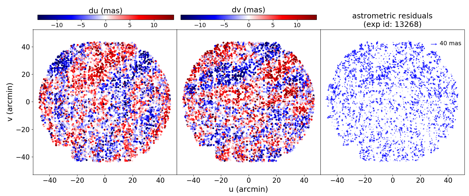
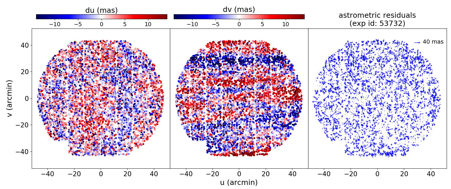
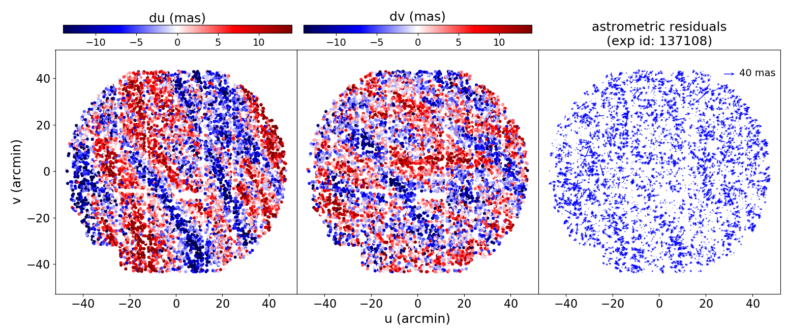
Figure 1: Distribution of astrometric residuals in right ascension ($du$, left column) and declination ($dv$, center column), and displayed as vectors (right column) for three individual exposures in $z$ band, as a function of position in the focal plane, indexed in arcmin with respect to the optical center of the camera. Gaps in the distributions are due to non-functionning CCD channels.

We then performed a simultaneous astrometric fit to the catalogs for the images for each night and each band separately – 5 to 15 images of the same field, with dithers of the order of a few arc minutes. The WCS’s for the input images are used to associate the detections of the same astronomical sources in different images. We simultaneously fit the geometrical transformations from pixel space to sky coordinates, and the coordinates of sources detected in at least two images. The fit is possible because we constrain a small fraction of the detected source positions to their Gaia (Data Release 2, Gaia Collaboration et al. 2018) positions on the date of observation; we call these sources the “anchors”. The geometric transformations are modeled as a per-CCD mapping of pixel coordinates to an intermediate plane coordinate, followed by a per-image mapping from this intermediate space to the tangent plane for this specific image. As such, this model is degenerate and we lift the degeneracy by imposing that one of the per-image transformations is the identity transformation. The rationale for this two-transformation model is that the per-CCD transformations capture the placement of the CCDs in the focal plane and the optical distortions of the instrument, while the per-image transformations capture the variations from image to image due to both flexion of the optics and atmospheric refraction. We initially model each transformation as a third-order polynomial – i.e., with 20 coefficients per transformation, or $\sim$2000 parameters for the instrument geometry, and 20 addtional parameters per image. The typical number of sources in a fit is $\sim$200,000, with a few thousands of these anchored to Gaia. The least-squares minimization takes advantage of the sparse nature of the problem and runs in about 60 s for the typical number of images (ten). The input uncertainties on the measured positions account for shot noise only; therefore, we add a position-error floor of 4 mas to all sources when computing the weight used in the least-squares fit to avoid over-fitting the bright sources.

The analysis presented in the next section uses the residuals of this fit as input. The typical rms deviation of the astrometric residuals for HSC is between 6 and 8 mas for bright sources (with the value depending on the band). The goal is to reduce the remaining dispersion and small scale correlations.

2.2 Astrometric residuals of HSC

We denote with $du$ and $dv$ the components of the astrometric residual field within the local tangent plane, in right ascension and declination, respectively. In Fig. 1, we show examples of the astrometric residuals, projected on the tangent plane, for three exposures. At this stage, the stochastic distortions affecting each exposure are modeled, as described above, with a small number of parameters (typically 20). The spatial correlation of the residuals, and the variability of the correlation from exposure to exposure, indicate that the parametrization with a third-order polynomial is not flexible enough to accommodate the observed variability. We see that the residuals exhibit a preferential direction that varies from exposure to exposure. This is very similar to the residuals observed in DES and shown in B17.

The spatial variations observed in the astrometric residuals exhibit preferential directions within an exposure; our hypothesis, as in B17, is that these anistropies are mostly due to atmospheric turbulence. In this case (as discussed in B17), the astrometric residual field follows the gradient of the optical refractive index of the atmosphere in the telescope beam, averaged over the integration time of the exposure. The two-point correlation function $\xi$ for the astrometric residual field has most generally two independent components, but only one if it is a gradient field and is curl free (Helmholtz’s theorem). The decomposition into a curl-free $E$-mode and a divergence-free $B$-mode of vector fields on the plane (B17) allows us to test the above hypothesis.

Following B17 (see appendix A in particular), we evaluate the two-point correlation functions $\xi_{+}$, $\xi_{-}$, and $\xi_{\times}$ for the astrometric residual field,

$$\xi_{+}(r,\beta) =\left<dX\left(\textbf{X}\right)e^{-i\beta}\left[dX\left(\textbf{X}+\textbf{r}\right)e^{-i\beta}\right]^{\star}\right>,$$ (1)

$$\xi_{-}(r,\beta)+i\xi_{\times}(r,\beta) =\left<dX\left(\textbf{X}\right)e^{-i\beta}dX\left(\textbf{X}+\textbf{r}\right)e^{-i\beta}\right>,$$ (2)

where $dX(\textbf{X})$ is the astrometric residual field on a complex form ($dX=du+idv$) measured at a position X on the focal plane, $r$ is the distance between two positions, and $\beta$ is the position angle of r. From $\xi_{+}$ and $\xi_{-}$ we find the correlation functions $\xi_{E}$ and $\xi_{B}$ correponding to the $E$- and $B$-modes of the field:

$$\xi_{E} =\frac{1}{2}\xi_{+}(r)+\frac{1}{2}\xi_{-}(r)-\int_{r}^{\infty}\frac{1}{r^{\prime}}\xi_{-}(r^{\prime})dr^{\prime}$$ (3)

$$\xi_{B} =\frac{1}{2}\xi_{+}(r)-\frac{1}{2}\xi_{-}(r)+\int_{r}^{\infty}\frac{1}{r^{\prime}}\xi_{-}(r^{\prime})dr^{\prime}$$ (4)

We evaluate the correlation functions by calculating the covariance between the astrometric residuals for pairs of sources, in bins of spatial separation between the sources. From these, we compute the binned version of $E$- and $B$-mode correlation functions. This involves an integral over separation (Eq. 37 in B17) that we evaluate by simply summing over each bin. With this binned estimation method, the integral of the correlation functions over angular separations is zero (see Appendix A).

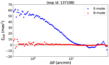
Figure 2: Typical $E$- and $B$-mode correlation functions for a single 300-s $z$-band exposure of HSC.

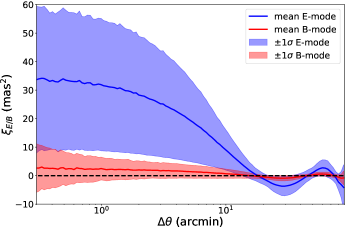
Figure 3: Average over all 2294 exposures of the $E$- and $B$-mode correlation functions. The blue and red shaded area represent respectively the standard deviation across nights of $E$- and $B$- mode.

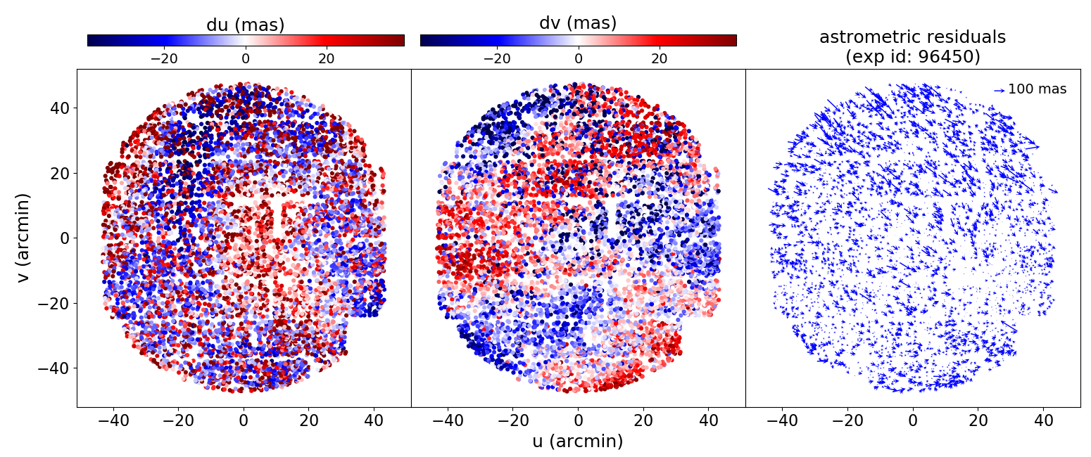
Figure 4: Distribution of astrometric residuals in right ascension ($du$, left) and declination ($dv$, center), and displayed as vectors (right), as a function of position in the focal plane. This $z$-band exposure corresponds to one of two nights when the focal plane was rotated through large angles during the course of the night.

In Fig. 2, we show the correlation functions corresponding to the $E$- and $B$-modes for the single exposure shown in the bottom row of Fig. 1). Figure 3 shows the mean value calculated over the 2294 exposures of the Deep and UltraDeep layers of the SSP. We observe that the $E$-mode correlation function is non-zero while the $B$-mode correlation function is compatible with zero. This is consistent with the result reported by DES in B17, for a different observing site and with a significantly different instrument. The HSC and DES results both indicate that the deplacement field can be described as the gradient of a scalar field, which is likely the average over the line-of-sight of the optical refractive index of the atmosphere, as argued in B17. We also note that the measured correlation function has negative values at large separations; this is unavoidable, because the integral of the correlation function is zero (see Appendix A). Moreover, the correlations that can be described by the fit of a third-order polynomial over the exposure data are much smaller than the observed correlation, and should have a correlation length of about 0.4^∘.

2.3 Difference between HSC and DES results

A notable difference between our results and those reported in B17 is the value of the correlation function as the angular separation approaches 0: Fig. 11 in B17, indicates a low-separation covariance of $E$-modes of the order of $80\ \text{milli-arcsec}^{2}$ while we observe a value of $33\ \text{milli-arcsec}^{2}$ for HSC; see Fig. 3. The fitting algorithms used to calculate the residuals are similar. However, there are two important quantitative differences: the exposure times are longer for HSC ($\sim$270 s vs. 90 s for DES), and the mirror diameter of the Subaru telescope is about twice as large as that of the Blanco Telescope (where DES observed). The variance attributed to atmospheric effects typically scales as the inverse of the exposure time (Heymans et al., 2012), while the dependence on aperture is more complicated, but favors larger apertures. Finally, the Subaru telescope is located at an elevation of 4400 m at the summit of Mauna Kea in Hawaii, while the Blanco telescope is at an elevation of only 2200 m at the Cerro Tololo Inter-American Observatory (CTIO) in Chile.

2.4 Nights with non zeros $B$-mode

Another significant difference between the HSC results reported here and those of DES are that the astrometric residuals in exposures for two HSC nights exhibit correlation functions with $B$-mode contributions that are not negligible compared to the $E$-mode contributions, and $E$-mode values much larger than typical. An example of the residuals for an exposure in such a night is shown in Fig. 4 and the corresponding correlation functions in Fig. 5. The Subaru telescope resides on an alt-azimuth mount; the field derotator mechanism rotates only the focal plane, while the wide-field corrector remains fixed with respect to the telescope. Our astrometric model indexes the optical distortions of the imaging system with respect to coordinates in CCD pixel space. Since in HSC, the image corrector rotates with respect to the CCD mosaic, any breaking of the rotational symmetry of the optical distortions will cause spurious astrometric residuals. As these residual only appear if exposures with different rotation angles are fit together, they tend to grow with the range of rotation angles involved in the fit. These residuals are not induced by the gradient of a scalar field, and hence are prone to similar amounts of $E$- and $B$-modes. The nights with large $B$-mode contributions are characterized by a large rotation of the focal plane over the course of the observations, mostly because the observations were spread over several hours, and sometimes most of the night. Our astrometric model does not compensate for this rotation (and neither does the one in B17), both because we were not aware of the details of the HSC mechanics before discovering these large rotations, and because the astrometry software we are using was originally developed for reducing the Canada-France-Hawaii Telescope (CFHT) Legacy Survey, and the CFHT has an equatorial mount. The fitted model would have to be heavily modified to account for these rotations, as noted in B17, for only the two night impacted by these large rotations. Most of our fits include images acquired over less than an hour and the whole rotation range is typically less than 20^∘.

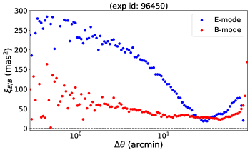
Figure 5: Typical $E$- and $B$-mode correlation function for the same exposure shown in Fig. 4, corresponding to one of two nights when the focal plane was rotated through large angles.

Other than these two nights with large focal plane rotations, the astrometric residuals exhibit a covariance pattern that can be mostly attributed to atmospheric turbulence. In the next section, we describe how we model these residuals.

3 Modeling astrometric residuals using anisotropic Gaussian processes

Spatial variations in the refractive index of the atmosphere can be described as a Gaussian random field, which must be stationary (that is, the covariance between values at different points depends only on their separation) because there is no special point in the image plane. We therefore model the astrometric residual field in the image plane as a Gaussian process (GP), which allows us to correct for astrometric residuals in the data, accounting for the correlations introduced by the Gaussian random field. In Sec. 3.1, we briefly introduce GPs, describe how the astrometric residual field can be modeled as a GP, and discuss possible strategies for optimization of the GP. In Sec. 3.2, we describe the method we use for the optimization of the GP hyperparameters, and our choice for the analytical correlation function. This GP interpolation was originaly developped for interpolating the atmospheric part of the PSF in the context of DES (Jarvis et al., 2021) and follow a similar scheme of interpolation.

3.1 Introduction to Gaussian processes

In this subsection, we give a brief overview of classical GP interpolation; a more detailed description can be found, for example, in Rasmussen & Williams (2006). A GP is the optimal method for interpolating a Gaussian random field. GP interpolation can be used for irregularly spaced datasets and, because it operates by describing the correlations between data rather than following a specific functional form, is very flexible. In practice, one must choose both the analytic form of this correlation function (also called a ”kernel”) and the parameters for this kernel (often called ”hyperparameters”) that describe the second-order statistics of the data.

A stationary Gaussian random field is entirely defined by its mean value (as a function of position) and its second-order statistics, which depend only on separation in position. We denote the (scalar) Gaussian random field as $y$ and its mean value as $y_{0}\equiv E[y]$, where $E[x]$ denotes the expectation value of the random variable $x$. Because the field is Gaussian (i.e., $y$ is Gaussian distributed at any position $X$), the distribution is Gaussian:

$$y\sim{\cal N}(y_{0},\xi(0)),$$ (5)

where $\xi$ is the correlation function:

$$\xi(X^{\prime}-X)\equiv{\rm Cov}(y(X),y(X^{\prime})).$$ (6)

In the context of modeling astrometric residuals, $y$ can be either of the components $du$ or $dv$, and $X$ is the coordinate in the local tangent plane. GP interpolation is a method for estimating the value of the field at arbitrary locations, given a realization of the field at a set of (usually different) locations. In practice, the kernel $\xi$ is unknown – or at least its parameters are unknown. We will discuss their determination in the next section. The covariance matrix for the data realization is calculated and used in the interpolation. The covariance matrix will be positive definite (which is required for it to be invertible in a later step) for any set of locations if and only if the correlation function $\xi$ has a positive Fourier transform (Bochner’s Theorem). This constrains the shape of possible correlation functions.

We now describe the practical interpolation method. We have a realization $y_{i}$ at positions $X_{i}$, and we assume for now that we know the kernel $\xi$. The covariance matrix $\boldsymbol{C}$ of the $\boldsymbol{y}$ realization is given by:

$$C_{ij}\equiv{\rm Cov}[y_{i}-y_{0}(X_{i})),y_{j}-y_{0}(X_{j})]=\xi(X_{j}-X_{i})+\delta_{ij}\sigma_{i}^{2},$$ (7)

where $\sigma_{i}$ is the measurement uncertainty of $y_{i}$.

The expectation of the Gaussian field at locations $\boldsymbol{y^{\prime}}$, given the values of $\boldsymbol{y}$ at locations $\boldsymbol{X^{\prime}}$, is (Rasmussen & Williams, 2006):

$$\boldsymbol{y^{\prime}}=\boldsymbol{\Xi}(\boldsymbol{X^{\prime}},\boldsymbol{y})\boldsymbol{C}^{-1}(\boldsymbol{y}-\boldsymbol{y_{0}})+\boldsymbol{y_{0}},$$ (8)

where $\boldsymbol{\Xi}$ is a matrix with elements defined by

$$\Xi(\boldsymbol{A},\boldsymbol{B})_{ij}\equiv\xi(\boldsymbol{A}_{i}-\boldsymbol{B}_{j}).$$ (9)

The covariance of the interpolated values is:

$$E\left[(\boldsymbol{y^{\prime}}-\boldsymbol{y_{0}}(\boldsymbol{X^{\prime}}))(\boldsymbol{y^{\prime}}-\boldsymbol{y_{0}}(\boldsymbol{X^{\prime}}))^{T}\right]=\\ \boldsymbol{\Xi}(\boldsymbol{X^{\prime}},\boldsymbol{X^{\prime}})-\boldsymbol{\Xi}(\boldsymbol{X^{\prime}},\boldsymbol{X})^{T}\boldsymbol{C}^{-1}\boldsymbol{\Xi}(\boldsymbol{X^{\prime}},\boldsymbol{X}).$$ (10)

We see from Eq. 8 that, in the absence of measurement uncertainties $\sigma_{i}$, the interpolated values at the training points $\boldsymbol{X}$ are just the $\boldsymbol{y}$ values with no uncertainties. This is because the interpolation method delivers the average expected field values given $\boldsymbol{y}(\boldsymbol{X})$ with covariance $\boldsymbol{C}$. In practice, the matrix $\boldsymbol{C}$ (defined in Eq. 7) is numerically singular or almost singular if there are no measurement uncertainties $\sigma_{i}$, even for sample sizes as small as 20; in the case of zero uncertainty, a small noise value should be added for the above expressions to be numerically stable.

The interpolation method is now well-defined, given a data realization and a choice of kernel. A commonly used kernel is the Gaussian kernel (also known as a squared exponential),

$$\xi\left(\textbf{X}_{1},\textbf{X}_{2}\right)=\phi^{2}\ \exp\left[-\frac{1}{2}\left(\textbf{X}_{1}-\textbf{X}_{2}\right)^{T}\textbf{L}^{-1}\left(\textbf{X}_{1}-\textbf{X}_{2}\right)\right],$$ (11)

where $\boldsymbol{X}_{1}$ and $\boldsymbol{X}_{2}$ correspond to two positions (in the focal plane for our case), $\phi^{2}$ is the variance of the Gaussian random field about the mean function $\boldsymbol{y_{0}}(\textbf{X})$, and the covariance matrix L is in general anisotropic since atmospheric turbulence typically has a preferred direction due to wind direction:

$$\textbf{L}=\left(\begin{matrix}\cos\alpha&\sin\alpha\\ -\sin\alpha&\cos\alpha\\ \end{matrix}\right)^{T}\left(\begin{matrix}\ell^{2}&0\\ 0&(q\ \ell)^{2}\\ \end{matrix}\right)\left(\begin{matrix}\cos\alpha&\sin\alpha\\ -\sin\alpha&\cos\alpha\\ \end{matrix}\right),$$ (12)

where $\alpha$ represents the direction of the anisotropy, $\ell$ represents the correlation length in the isotropic case, $q$ is the ratio of the semi-major to semi-minor axes of the ellipse associated with the covariance matrix.

Although a Gaussian kernel is often used, we can choose an analytical form for the kernel based on empirical considerations and/or the relevant physics. Both the functional form of the kernel and the hyperparameters associated with the kernel determine the interpolated estimates. Once the kernel shape is chosen, the parameters can be determined with a maximum likelihood fit, where the likelihood of the realization $\boldsymbol{y}$ (of size $N$) is defined by

$${\cal L}=\frac{1}{{\sqrt{2\pi}}^{N}}\times\frac{1}{\sqrt{\det(\boldsymbol{C})}}\times\exp\left(-\frac{1}{2}\left(\textbf{y}-\textbf{y}_{0}\right)^{T}\boldsymbol{C}^{-1}\left(\textbf{y}-\textbf{y}_{0}\right)\right).$$ (13)

Maximizing this expression with respect to the parameters of $\xi$ that define $\boldsymbol{C}$ (via Eq. 7) is numerically cumbersome because it involves many inversions (in practice, factorizations) of the covariance matrix $\boldsymbol{C}$, which has the size of the “training sample” y. The factorisation (for example, the Cholesky decomposition) also trivially delivers the needed determinant. The time to compute such a factorisation scales as ${\mathcal{O}}\left(N^{3}\right)$, where $N$ is the size of the training sample $\boldsymbol{y}$. It is possible to speed up the inversion of the matrix $\boldsymbol{C}$ in Eq. 13 under certain assumptions. For example, Ambikasaran et al. 2015 propose to speed-up the matrix inversion from ${\mathcal{O}}\left(N^{3}\right)$ to ${\mathcal{O}}\left(N\log^{2}(N)\right)$ based on a special decomposition of the matrix (HODLR). Other methods achieve ${\mathcal{O}}\left(N\right)$ under certain assumptions about the analytical form of the kernel and by being limited to one dimension (Foreman-Mackey et al., 2017).

Here, we follow another route, which relies on the good sampling provided by the training sample. From the smoothness of the measured correlation function in Fig. 2, we can conclude that the average distance to the nearest neighbors is much smaller than the correlation length. Therefore, we can estimate the anisotropic correlation function directly from the data. The practical implementation is described in the next section.

Figure 6: Typical computational time necessary to determine hyperparameters as a function of the number of data points used during training for a classical maximum likelihood method using Cholesky decomposition (red triangles) and when using the two-point correlation function computed by TreeCorr (blue circles). The typical number of training points for astrometric residuals modeled using GPs is between $\sim 10^{3}$ and $\sim 10^{4}$.

3.2 Hyperparameter estimation using the two-point correlation function

Estimating the kernel of a stationary GP directly from the two-point statistics was pioneered in the field of geostatistics (see Cressie 1992 for example). The time to compute the two-point correlation function naively scales as ${\mathcal{O}}\left(N^{2}\right)$; however, faster approaches have been developed. We use a package called TreeCorr (Jarvis et al., 2004), which evaluates covariances in distance bins for large datasets. Our implementation of the estimation of hyperparameters using TreeCorr can be found online. The computational time for TreeCorr depends on the bin size (see section 4.1 of Jarvis et al. 2004), and it proves particularly efficient for data sets of a size relevant to PSF interpolation, where it scales roughly linearly with the number of input data points. Figure 6 shows the computational time for the maximum likelihood approach and the estimation of hyperparameters based on the binned two-point correlation function using TreeCorr, as a function of the number of data points; the latter technique is several orders of magnitude faster for the training sample sizes we are contemplating (between $\sim 10^{3}$ and $\sim 10^{4}$).

We estimate the covariance matrix of the binned two-point correlation function via a bootstrap (done on sources). This measured covariance matrix is then used in the fit of the analytical model for the kernel to the measured two-point correlation function in a non-diagonal least-squares minimization. These three steps (binned two-point correlation function, bootstrap covariance matrix, least-squares fit) are included in the computational times shown in Fig. 6.

Although the Gaussian kernel is often used for GP interpolation, for ground-based imaging, a kernel profile with broader wings is expected to provide a better description of the longer-range correlations present in PSF dominated by atmospheric turbulence (see, for example, Fig. 2 in Roddier 1981). To account for the clear anisotropy in the correlation function, we use an anisotropic von Kármán kernel as proposed in Heymans et al. 2012 to describe the observed spatial correlations of PSF distortions for CFHT and is parametrised as

$$\xi\left(\textbf{X}_{i},\textbf{X}_{j}\right)=\phi^{2}\times\left[\left(\textbf{X}_{i}-\textbf{X}_{j}\right)^{T}\textbf{L}^{-1}\left(\textbf{X}_{i}-\textbf{X}_{j}\right)\right]^{\frac{5}{6}}\times\\ K_{-5/6}\left[2\pi\left(\textbf{X}_{i}-\textbf{X}_{j}\right)^{T}\textbf{L}^{-1}\left(\textbf{X}_{i}-\textbf{X}_{j}\right)\right],$$ (14)

where the notation is the same as for Eq. 11 and $K$ is the modified Bessel function of the second kind. At large separations, $\xi$ decays exponentially. We show in Fig. 7 Gaussian and von Kármán kernels of similar widths. As we will soon show, a von Kármán kernel reduces the residuals more efficiently than a Gaussian kernel.

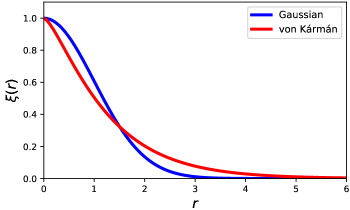
Figure 7: Gaussian kernel compared to the von Kármán kernel that is used in this analysis. The width of the latter was determined by a least-squares fit to the former.

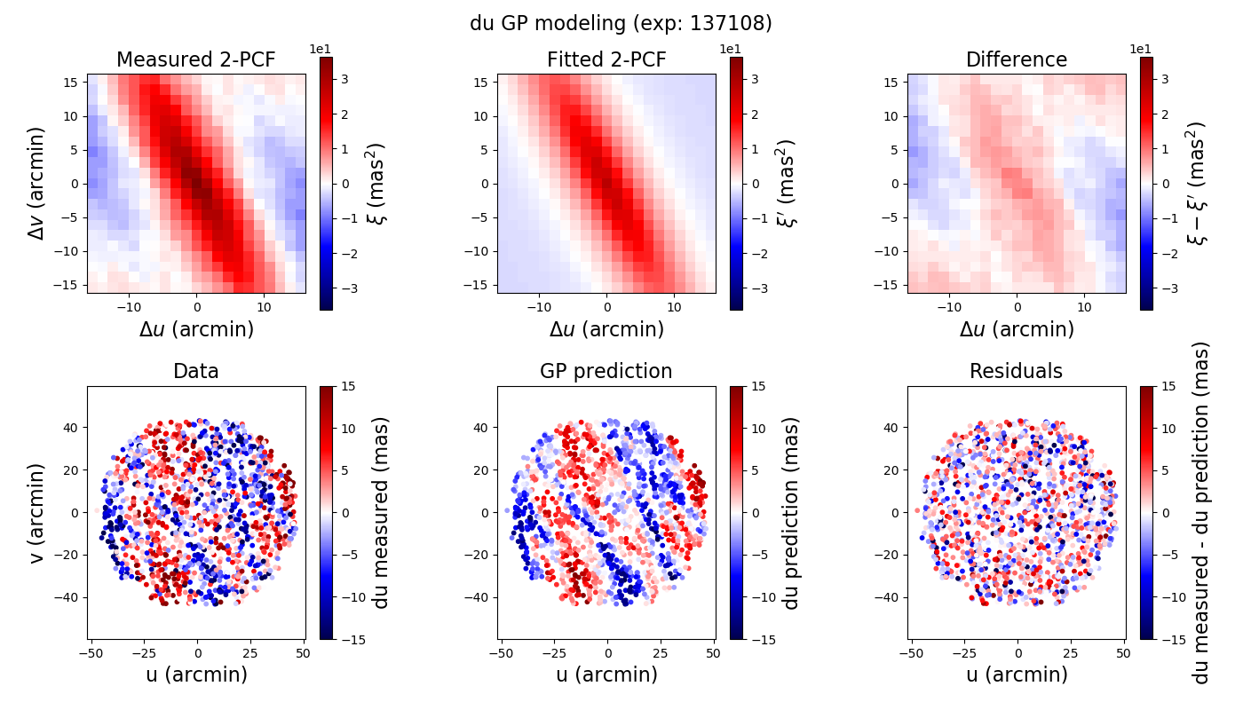
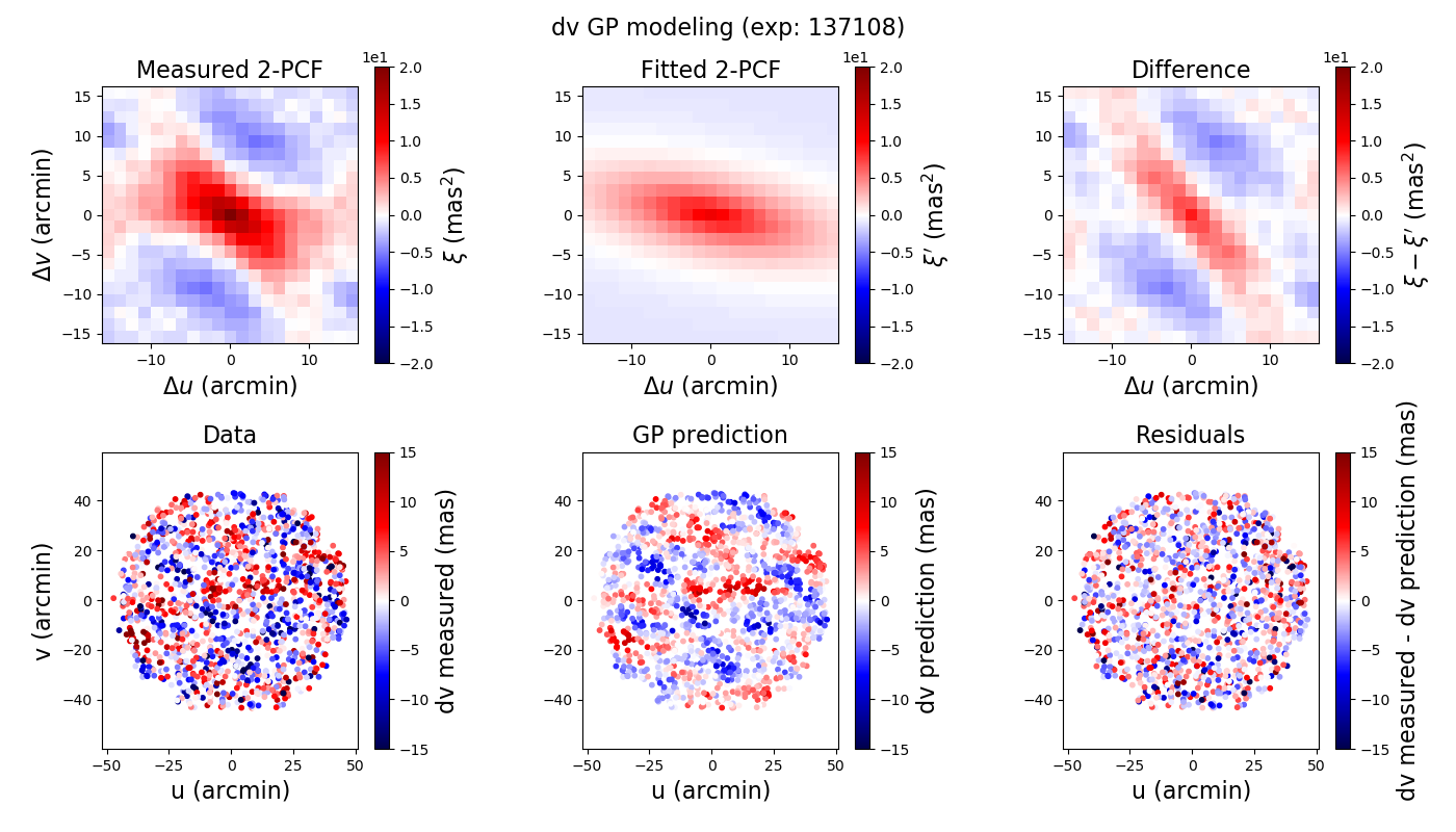
Figure 8: GP fit of astrometric residuals for a single 300-s $z$-band exposure. The fit is done independently for each component of the vector field. The top six plots show results for the $du$ component, and the bottom six plots for the $dv$ component. The plots in the top row within each group illustrate how the hyperparameters are determined from a von Kármán kernel (center plot) fit to the measured two-point correlation function calculated for 80% of the training sample (left plot); the difference between the measured two-point correlation function and the best-fit von Kármán kernel is shown in the right-most plots. The plots in the bottom row within each group of six represent the variation across the focal plane of the measured component of the astrometric residual field, the astrometric residual field predicted by the GP using the best-fit hyperparameters, and the difference between measure and fit, projected in the local tangent plane for the 20% of sources in the validation sample.

One may wonder why we rely on a parametrized form of the kernel, typically with a small number of parameters (four here), rather than using a more empirical fit (for example with spline functions) of the measured correlation function. As discussed earlier, a correlation function should have a positive Fourier transform and, if it does not, the covariance matrix of observations (Eq. 7 for $\sigma_{i}=0$) is not positive-definite for all realizations. Therefore, when smoothing the measured correlation function, one should restrict the outcome to functions with positive Fourier transforms. Splines cannot in general be guaranteed to have positive Fourier transforms. Both Gaussian and von Kármán kernels fulfill this requirement, so we only consider these two models. We note that a maximum likelihood approach faces the same constraint of having a correlation function with a positive Fourier transforms.

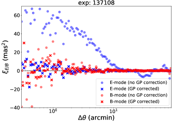
Figure 9: Correlation functions corresponding to $E$- (blue) and $B$- (red) modes of the astrometric residual field on the validation sample for a representative exposure (one of three exposure shown in Fig. 1), before applying the GP interpolation correction (circles) and after correction (crosses)

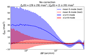
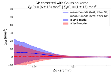
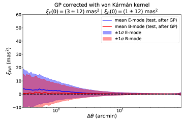
Figure 10: Average over all 2294 exposures of the $E$- and $B$-mode correlation functions, calculated on the validation sample, for different modeling choices. Top: Correction from GP interpolation is not applied. Middle: correction from GP interpolation is applied using a Gaussian kernel. Bottom: correction from GP interpolation is applied using a von Kármán kernel. For all those plots, the blue and red shaded area represent respectively the standard deviation across nights of $E$- and $B$- mode.

3.3 Difference with DES GP modeling

We now describe the main differences with the approach chosen in F20. First, we do not enforce the model to describe a gradient field; rather we model and fit independently the two spatial components. In F20, the authors eventually optimize the kernel hyperparameters in order to minimize the average covariance on small angular scales, while we simply fit the hyperparameters to the empirical covariance. We speculate whether this optimization is necessary and whether it will be viable when it comes to large scale production as required by the processing of Rubin Observatory data. Second, the anisotropy of the correlations in F20 is entirely attributed to the wind-driven motion of a static phase screen during the exposure, and we have not tested whether this assumption improves our results. Third, We model the correlation function with four parameters, while F20 use five, where the fifth parameter is the outer scale and we expect its influence on the correlation function to be small. Finaly, we have not rejected outliers in the GP fit; i.e., sources exhibiting large a posteriori residuals are not removed from the training sample, but a priori outliers have been removed.

4 Correcting astrometric residuals using anisotropic Gaussian processes

We apply GP interpolation to the astrometric residuals for the 2294 exposures of the SSP in the five bands. We train the GP on the unsaturated sources with magnitudes brighter than 20.5 AB mag. The residuals are clipped at 5-$\sigma$ during the prior astrometric fitting process but, in contrast with F20, we do not clip in the GP fit. We fit the two projections of the residuals as independent GPs, and ignore cross correlations.

As discussed earlier, GPs simply reproduce the input data if interpolation at an input data point is requested, at least in the absence of measurement noise. Therefore, in order to use residuals to evaluate the GP performance in an unbiased way, we randomly select a “validation sample” consisting of 20% of the sources fully qualified for training, that we exclude from the training sample. We then compute the GP interpolation for all sources used in the astrometry (i.e., all sources with an aperture flux delivering a signal-to-noise ratio greater than 10). The performance tests described in this section (unless otherwise specified) are computed only on this validation sample.

The result of the GP modeling of the astrometric residual field for a single exposure in $z$-band is shown in Fig. 8 (see caption for detail). The measured correlation functions have negative lobes because they integrate to zero. The positive analytical function cannot obviously reproduce those negative parts. We add a constant floor $k$ in order to allow the kernel to have negative lobes and to not bias hyperparameters estimation. Consequently, the following equation is minimized in order to find the best set of hyperparameters $\boldsymbol{\theta}$:

$$\chi^{2}=\left(\boldsymbol{\xi}-\hat{\boldsymbol{\xi}}(\boldsymbol{\theta})-k\right)^{T}\boldsymbol{W}\left(\boldsymbol{\xi}-\hat{\boldsymbol{\xi}}(\boldsymbol{\theta})-k\right)\ ,$$ (15)

where $\boldsymbol{\xi}$ is the measured two-point correlation function, $\hat{\boldsymbol{\xi}}$ is the analytical kernel (gaussian or von Kármán), $\boldsymbol{W}$ is the inverse of the covariance matrix of the measured two-point correlation function, and $k$ which is the constant not taken into account when computing the final kernel and consequently when computing the GP interpolation (Eq. 8). The von Kármán kernel fits well the principal direction of the anisotropy and delivers a reasonable correlation length. However, one can see that by looking at the two-point correlation function residuals on the third row of Fig.  8 that the von Kármán profile does not fit perfectly the observed kernel, even if it does a better job than the classic Gaussian kernel (see below). A room for improvement would be to have a more flexible kernel to describe the observed two-point correlation, such as a spline basis, but lies beyond the scope of this analysis.

We show in Fig. 9 the correlation functions for the $E$- and $B$-modes of the astrometric residual field calculated for the validation sample in a representative exposure (same as the one presented in Fig. 8), before and after GP modeling and interpolation with a von Kármán kernel. We see a significant reduction in $E$-mode correlation function after GP interpolation.

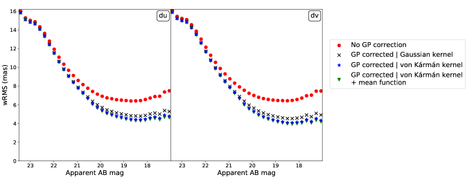
Figure 11: Weighted RMS of astrometric residuals as a function of apparent AB magnitude of the source for each component of the astrometric residual field. Four models are compared: no correction from a GP interpolation (red circles), correction from a GP interpolation with a Gaussian kernel (black crosses), correction from a GP interpolation with a von Kármán kernel (blue stars), and correction from a GP interpolation with a von Kármán kernel and the mean function computed as described in Sec. 5 (green triangles, hidden underneath the blue ones).

We show in Fig. 10 the $E$ and $B$-mode correlation functions calculated for the validation sample and averaged over all 2294 exposures, before (top plot) and after GP interpolation with a Gaussian kernel (center plot) and a von Kármán kernel (bottom plot), together with the $\pm 1$-$\sigma$ spread over exposures. GP interpolation reduces the magnitude of the correlation function by almost one order of magnitude, from 30 mas² to 3 mas² at small scales. The von Kármán kernel performs better than the Gaussian kernel. We can also see the improvement by comparing the dispersion of the astrometric residuals with the flux as in Fig. 11. As for the $E$-mode reduction, it can be seen that after correcting by the GP interpolation, GP reduces the dispersion by a factor of two and the von Kármán kernel does a better job than the classical Gaussian kernel by $\sim 20\%$ in rms.

We investigated whether the a posteriori residuals are sensitive to the size of the training set, and found no compelling differences between results for exposures with 2000 and 6000 training sources. We interpret this as an indication that the modeling is not limited by the image plane sampling or the shot noise affecting position measurements, but rather by the ability of the kernel to describe the correlation. Therefore, reducing the number of training points is an immediate avenue to reducing computational demands, and further work should focus on modeling of the kernel.

5 Average residuals in CCD coordinates

Sensor effects that are not modeled with the GP (e.g., fabrication defects in the CCD, or distortions in the drift fields) can appear in an image of the average residuals over the focal plane. In Fig. 12, we show the average value over all the exposures of the two components of the residuals for three representative CCDs. One can see two main types of defects: so-called ”tree rings”, and ”scallop-shaped” structures near the edges of the sensors. The former are commonly attributed to the variation in the density of impurities, with a symmetry due to how the crystals are grown. The latter are likely due to mechanical stresses applied to the silicon lattice, induced by the binding of the sensor to its support structure. The DECam sensors exhibit similar defects, as shown in B17, but at about an order of magnitude larger scale. The sizes of the tree-ring residuals are $\sim 2$ mas for HSC and $\sim 13$-26 mas for DECam (Plazas et al., 2014). We have not been able to find in the literature previous mention of these tiny defects on HSC sensors. The rms astronomical residuals associated with the scallop-shaped features in the images for the HSC CCDs are $\sim$10 mas – larger than those associated with the tree-ring features.

In order to clearly see these small effects (mostly below 10 mas), we averaged all bands together since the signal in individual bands is very noisy. We expect that the patterns in each band will differ only on a global scale due to the variation with wavelength of the average conversion depth of photons in silicon. We mildly confirm that redder bands have weaker patterns, as expected, but we could not devise a robust measurement of ratios between bands. Averaging in larger spatial bins smears the smaller structures. If we apply these patterns as a mean function of the GP, the improvement of the residuals (both in variance and covariance) is below 1 mas² (cf. Fig. 11). However, recomputing the mean function and taking it into account in the GP modeling allows us to remove most of the patterns observed in individuals CCDs as shown in Fig. 13.

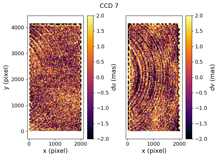
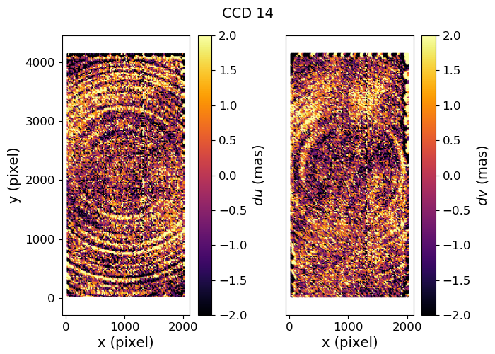
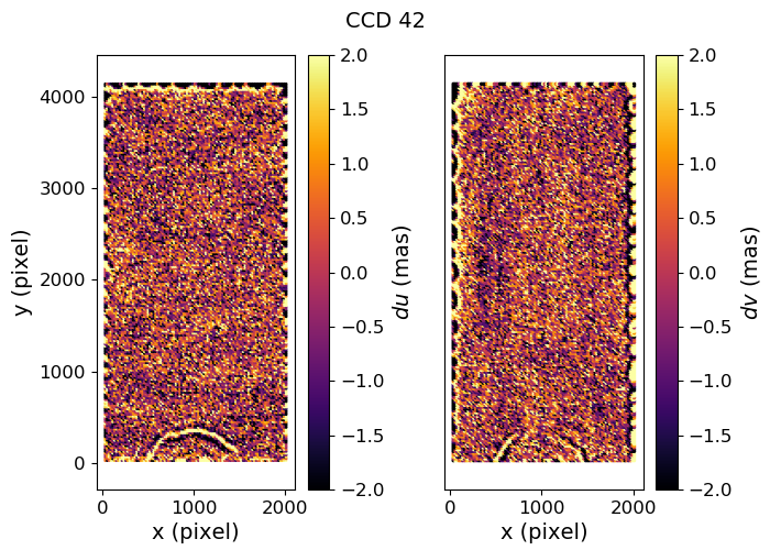
Figure 12: Average of the astrometric residual field for each component projected in pixel coordinate for 3 different chips with some characteristic features that can be also found on the other chips.

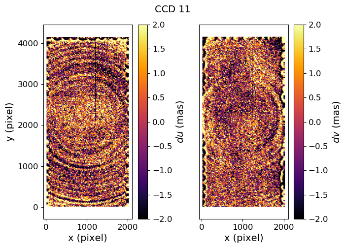
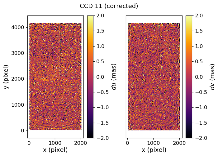
Figure 13: The average of the astrometric residual field for each component projected in pixel coordinates for a given chip, before and after including the average in the GP model as a mean function.

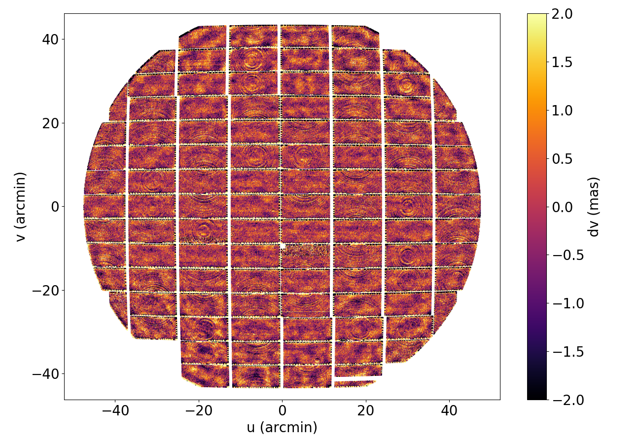
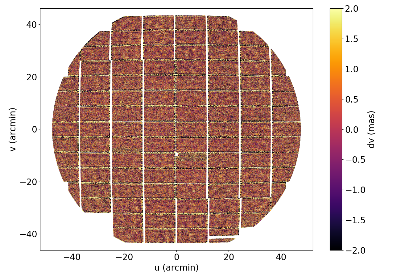
Figure 14: Average of the astrometric residual field for each component (top row: du, bottom row: dv) projected in the local tangent plane. The per sensor transformation from pixel coordinates to tangent plane is a second-order polynomial in the left column, vs a fifth-order polynomial in the right column.

The HSC instrument is characterized by a rapid evolution of the plate scale in the outer part of the focal plane: the linear plate scale varies by 10% between the center and the edge of the field, and 70% of this variation is concentrated in the outer 30% radius. In order to verify that our modeling can cope with this variation, we plot the residuals in the whole focal plane, in order to check for systematic residuals at the few mas level in Fig. 14. The model consists of one polynomial transformation per sensor from pixel coordinates to the tangent plane, common to all exposures. We see in Fig. 14 that there are residuals when using third-order polynomials per CCD, which disappear with fifth-order polynomials. However, all the astrometric residuals used in the GP modeling used the third-order polynomials per CCD.

6 Impact of correlations in astrometric residuals on cosmic shear measurements

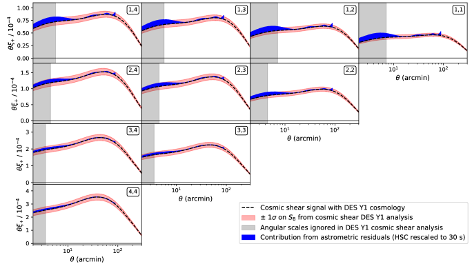
Figure 15: Tomographic cosmic shear signal (presented here only for $\xi_{+}$) measured by DES Y1 (black curve) and compared to the expected signal introduced by the spatial correlations of astrometric residuals due to the atmosphere by rescaling HSC data on 30 s LSST exposure (blue area). If not corrected, the effect of astrometric residuals in LSST on galaxy shapes will bias the shear signal. This is a lower limit as the HSC site is at a higher altitude that the Rubin Observatory and the effective size mirror of HSC is bigger than the Rubin Observatory telescope. With the GP correction proposed in this current analysis, we expect to be able to lower it by orders of magnitude.

We explained above that Rubin Observatory will need to model the astrometric distortions from the atmosphere because of the short exposures (two back-to-back 15-s exposures) defined in the current observing plan. We measure for HSC a small-scale covariance in astrometric residuals of about 30 mas² for an average exposure duration of 270 s. The Rubin Observatory telescope has a smaller effective primary mirror area than the Subaru telescope and is located at a lower elevation, so we expect atmospheric effects to be more significant at Rubin Observatory. Neglecting these differences, and assuming that covariances vary only as the inverse of the exposure time, we would expect 540 mas² and 270 mas² of small-scale covariance on average for Rubin Observatory exposures of 15 s and 30 s, respectively. These covariances affect in a coherent way the astrometric residuals, and can extend up to 1 degree, along the major axis of the correlation function. Those may affect the measurement of shear, and we will now provide a rough estimate of the shear correlation purely due to these turbulence-induced residuals, for 30-s exposures in the Rubin Observatory, assuming they are not mitigated.

Measuring shear without co-adding images requires measuring second moments using galaxy positions averaged over images, because the position noise biases the second moments (this is the so-called noise bias). Using average positions is particularly required for the Rubin observatory where the final image depth is obtained from hundreds of short exposures in each band. In order to evaluate the effect of displaced positions on cosmic shear signal, we shift positions coherently on small spatial scales by $dx$ in a single exposure. Using a Taylor expansion, we derive the shear offset in the astrometric residual direction to be

$$\delta\gamma\simeq\frac{1}{4}\left(\frac{dx}{\sigma_{g}}\right)^{2},$$ (16)

independent of the size of the PSF, where $\delta\gamma$ is the shear bias and $\sigma_{g}$ denotes the r.m.s. angular size of the galaxy, and $dx$ the (spurious) position shift. The general expression, accounting for actual directions, reads

$$\delta\gamma_{1}+i\delta\gamma_{2}\simeq\frac{1}{4}\left(\frac{dx+i\ dy}{\sigma_{g}}\right)^{2}.$$ (17)

where $\gamma_{1}$ describes shear along the $x$ or $y$ axes, and $\gamma_{2}$ the shear along axes rotated by $45^{\circ}$, as defined in Schneider et al. (2006). Therefore, the shear covariances induced by covariances of position offsets involve the covariance of squares of position offsets. For centered Gaussian-distributed variables $X$ and $Y$, we have

$$\textrm{Cov}(X^{2},Y^{2})=2\left[\textrm{Cov}(X,Y)\right]^{2},$$ (18)

which allows us to relate the correlation function of shear to the correlation function of position offsets. In order to evaluate the impact of spatially correlated position offsets on measured shear spatial correlations, we consider the smallest galaxy sizes used in DES Y1 (Zuntz et al., 2018), which have $\sigma_{g}\simeq 0.2^{\prime\prime}$. Their shear will experience an additive offset of $\sim 1.6\times 10^{-3}$ (for a small scale correlation of 270 mas²), which will bias the shear correlation function by $\sim 6\times 10^{-6}$, which is about half of the expected cosmic shear signal at $z\sim 0.5$ and 10 arcmin separation.

In Fig. 15, we display both the expected cosmic shear signal and the contribution from the position offsets derived from the average HSC measurement, scaled to 30-s exposures, assuming those offsets are not mitigated. This prediction assumes that the shear is measured on individual exposures, using a common average position with no GP modeling and correction of atmospheric displacements. The cosmic shear signal in Fig. 15 is computed in the four tomographic bins used in the cosmic shear analysis of Troxel et al. 2018; the shear correlation functions $\xi_{+}$ are computed using the Core Cosmology Library (Chisari et al., 2019) with the fiducial cosmology result from Troxel et al. 2018 (black curve in Fig. 15). The comic shear signal presented in Fig. 15 takes into account the non-linearity of the matter power spectrum and the spatial correlations introduced by the intrinsic alignment as in Troxel et al. 2018. For a representation of the current knowledge of the cosmic shear signal, we indicate in Fig. 15 with a dark region around the cosmic shear correlation function the variations on $S_{8}$ ($\sigma_{8}(\Omega_{m}/0.3)^{0.5}$) of $\pm 0.027$, which represent the $\pm 1\sigma$ uncertainty from the fiducial cosmic shear analysis of Troxel et al. 2018. The regions shaded in red in Fig. 15 in each tomographic bin represent the angular scales that were removed in the Troxel et al. 2018 analysis because they could be significantly biased by baryonic effects. The blue area in Fig. 15 in each of the tomographic bins represent the contribution to the cosmic shear signal due to the average spatial correlations of the astrometric residuals due to atmospheric turbulence scaled from the HSC average measurement to 30-s exposures. This adds to shear a contribution comparable to the DES Y1 uncertainty, which is considerably larger than the LSST precision goal. These correlated position offsets were not an issue for previous surveys like DES because the variance of the astrometric residuals in DES is 3 times lower than that expected for LSST, and therefore the contribution to the shear correlation function is 10 times lower since is scales as the square of the variance. It is unlikely that the wind direction projected on the sky would average out this effect, because the wind direction at an observatory has a preferred direction, on average. If we are able to reduce the position covariances down to a few mas², the effect on the shear correlation functions becomes 2 to 3 orders of magnitude smaller than the cosmic shear signal itself.

We have described a measurement scheme where galaxy positions are affected by turbulence-induced offsets. If one performs an image co-addition prior to shear measurement, the co-addition PSF will account for the position offsets, and hence the shear measurements may be free of the offsets described above. This is true for regions covered by all exposures, but there are discontinuities of both PSF and the atmospheric-induced shear field where the number of exposures involved in the co-addition changes. Note also that the atmospheric-induced offsets cause a PSF correlation pattern that may prove difficult to discribe accurately. Therefore, for short exposure times, even if one co-adds images and then measures shear, one probably has to accurately model the spatial correlations in the atmospheric-induced position shifts down to arc-minute scales.

7 Conclusions

We have studied astrometric residuals for bright stars measured in exposures acquired with the HSC instrument on the Subaru telescope, and find that these residuals are dominated by $E$-modes. We have developed a fast GP interpolation method to model the astrometric residual field induced by atmospheric turbulence. We find that a von Kármán kernel performs better than a Gaussian kernel, and the modeling reduces the covariances of neighboring sources by about one order of magnitude, from 30 mas² to 3 mas² in variance, and the variances of bright sources by about a factor of 2. Those reductions using GP interpolation are really similar to recent result published in F20 with the DES dataset. Based on simulations of atmospheric distortions above the Rubin Observatory telescope, we find that, for short exposures, the correlated astrometric residuals may cause a spurious contribution to shear correlations as large as the cosmic signal. Mitigating these turbulence-induced offsets, possibly along the lines we have sketched in this paper, will be necessary for cosmic shear analyses. We have shown that the spatial correlation of astrometric residuals can be significantly lowered by modeling and then correcting these residuals using GP interpolation. We find that it is necessary to incorporate this modeling in the astrometric fit itself (as opposed to the GP interpolation done in post-processing and described in Sec. 3 and Sec. 4) in order to achieve more precise and accurate average source positions and pixel-to-sky transformations. The post-processing can be done along the lines sketched in the presented analysis, namely finding the hyperparameters for a chosen form of the kernel using the two-point correlation function of residuals for each exposure and generating the astrometric residual field from the current residuals using Eq. 8. Our astrometric model describes the average optical distortions of the instrument down to the mas level, and we have been able to detect the 1 to 10 mas scale CCD-induced image distortions that causes systematic astrometric residuals of the sources.

Appendix A Integral of the correlation function

We demonstrate here that the integral of the correlation function for astrometric residuals is null because the average of the astrometric residual field is null per construction of the model. In the continuous limit, the correlation function is defined as

$$\xi(r)=\int f(x-r)f(x)dx.$$ (19)

Consequently, the integral of the correlation function is

$$\int\xi(r)dr=\int\int f(x-r)f(x)dxdr.$$ (20)

Making the change of variables $X=x-r$, we have

$$\int\xi(r)dr=\left(\int f(X)dX\right)\left(\int f(x)dx\right).$$ (21)

For the specific case of astrometric residuals, the average of the astrometric residual field is constructed to be zero; consequently, we have

$$\int f(x)dx=0,$$ (22)

which means the integral over the correlation function is zero:

$$\int\xi(r)dr=0.$$ (23)