Quasi-normal modes of rotating black holes in Einstein-dilaton Gauss-Bonnet gravity: the first order in rotation

Abstract

Gravitational spectroscopy - the measurement of the quasi-normal modes of a black hole from the ringdown signal of a binary black hole coalescence - is one of the most promising tools to test gravity in the strong-field, large-curvature regime, but without the knowledge of the black hole quasi-normal modes in specific cases of modified gravity theories, only null tests of general relativity are possible. More specifically, we need to know the modes of rotating black holes, because typical compact binary mergers lead to black holes with large spins. In this article we compute, for the first time, the gravitational quasi-normal modes of rotating black holes in a modified gravity theory, up to first order in the spin. We consider Einstein-dilaton Gauss-Bonnet gravity, one of the simplest modifications of general relativity in the large-curvature regime. We find that the shifts in the mode frequencies and damping times due to general relativity modifications are significantly magnified by rotation.

I Introduction

The detection of gravitational waves (GWs) from a binary black hole (BH) coalescence [1] opened the possibility of testing general relativity (GR) in the strong-field regime of gravity [2]. While the inspiral signal is very sensitive to dipolar emission due to additional polarizations (see e.g. [3, 4]), the ringdown signal, i.e. the emission of GWs from the oscillating BH born in the merger, carries the imprint of possible GR modifications in the large-curvature regime. The merger signal may also be a very sensitive probe of strong-field GR modifications, but the necessary theoretical modelling of this stage is extremely challenging; indeed, in order to perform numerical relativity simulations of binary BH coalescence in a modified gravity theory, we need to develop a well-posed and well-behaved formulation of the time-evolution problem (see e.g. [5, 6, 7, 8, 9, 10, 11]).

The study of the ringwdown is also technically challenging, but it does not present fundamental issues. After the merger, the waveform is accurately described by a superposition of damped oscillations, the quasi-normal modes (QNMs) of the BH [12, 13, 14]. The frequencies and damping times of the modes in the observed signal can be compared with the predictions of GR, leading to null tests of GR. If a deviation is observed, a comparison with the predictions of specific modifed gravity theories would give information on the nature of the modification. This idea has been called “gravitational spectroscopy” [15, 16, 17] (see also [18] and references therein).

Gravitational spectroscopy requires an a priori theoretical knowledge of the QNMs in modified gravity theories. Although the computation of the QNMs is conceptually simple - it requires the numerical integration of the field equations linearized around the stationary BH background, imposing appropriate boundary conditions at the horizon and at infinity - few results are currently available in the literature. The QNMs of static, non-rotating BHs have been computed for a certain number of modified gravity theories [19, 20, 21, 22, 23, 24, 25, 26] (other computations refer to oscillations of a test scalar field, and thus are not relevant for gravitational spectroscopy). A different possible approach to study BH QNMs in modified gravity is that of modifying the radial potential in the perturbation equations, and computing how these deformations affect the QNM frequencies and damping times [27, 28].

The main limitation of these studies is that they only refer to static, non-rotating BHs. Conversely, astrophysical BHs do rotate; due to angular momentum conservation, even when the two BHs in the binary have negligible spin, the final BH has – for a comparable-mass binary- $\bar{a}=J/M^{2}\sim 0.7$ (where $M,J$ are the mass and angular momentum of the BH, respectively). Gravitational spectroscopy, then, requires the previous knowledge of QNMs of stationary, rotating BHs in modified gravity theories. This article is, to our knowledge, the first computation of rotational corrections of BH QNMs in a modifed theory of gravity.

Several modifiations of GR have been proposed, but most of them can be reformulated in terms of the addition of extra polarizations - such as a scalar field - to the gravitational sector of the theory [29]. Some of these scalar-tensor theories modify the weak-field regime of gravity, and thus are strongly constrained by binary pulsar observations [30, 29]. This is not the case for Einstein-dilaton Gauss-Bonnet (EdGB) gravity, one of the simplest scalar-tensor theories which modifies the strong-field, large-curvature regime of gravity. EdGB gravity is described by the action [31, 32]:

$$S=\int d^{4}x\frac{\sqrt{-g}}{16\pi}\left(R-\frac{1}{2}\partial_{\mu}\phi\partial^{\mu}\phi+\frac{\alpha_{\rm GB}}{4}e^{\phi}\mathcal{R}^{2}_{\rm GB}\right)+S_{\rm m}$$ (1)

where

$$\mathcal{R}^{2}_{\rm GB}=R_{\mu\nu\rho\sigma}R^{\mu\nu\rho\sigma}-4R_{\mu\nu}R^{\mu\nu}+R^{2}$$ (2)

is the Gauss-Bonnet term, and $S_{\rm m}$ is the matter Lagrangian. This theory - which naturally arises in some low-energy truncations of string theories - belongs to the class of Horndeski gravity [33, 34], the scalar-tensor theories with second-order-in-time field equations (which are thus free from the Ostrogradsky instability). Remarkably, while in several scalar-tensor theories the no-hair theorem of GR is satisfied, and thus stationary BHs are described by the Kerr solution, BHs in EdGB gravity always have a non-trivial scalar field profile, and thus are different than in GR.

The Gauss-Bonnet term (2) is quadratic in the curvature and thus is negligible in weak-field regions of spacetime. Thus, EdGB gravity is not constrained by binary pulsar observations: the deviations from GR only show up in very strong-field processes such as the merger and the ringdown of a binary BH coalescence. This makes EdGB gravity a perfect candidate for gravitational spectroscopy. Currently, the strongest bound on the coupling constant $\alpha_{\rm GB}$ arises from the theoretical bound in Eqs. (8), (9): the existence of the lightest BH observed, J1655-40, with mass $M\simeq 5.4\,M_{\odot}$ implies $\sqrt{\alpha_{\rm GB}}<6.6$ Km; if the secondary object in GW190814, with mass $M\simeq 2.6M_{\odot}$, turns out to be a BH, then $\sqrt{\alpha_{\rm GB}}<3.3$ Km [35] .

QNMs of static, non-rotating BHs in EdGB gravity have been computed in [23]. The modes of rotating BHs have only been estimated using the so-called “geodesic correspondence” [39, 40, 41], which states that the QNMs can be approximately computed in terms of the orbital frequencies near the light ring, and the approximation is better for larger values of the harmonic index $l$. The geodesic correspondence has been formally proved for Kerr BHs in GR, but there is no proof of it in modified gravity theories. Moreover, while the geodesic approximation predics the QNMs to be isospectral - i.e., to coincide for perturbations with polar and axial parities - we know that in theories such as EdGB gravity and Chern-Simons gravity [42] the QNMs are not isospectral [20, 23], thus the geodesic approximation is violated (see also [43] for a computation of the QNMs of non-rotating BHs in EdGB gravity within the geodesic approximation). In particular, it is reasonable to expect such violation when the spacetime metric is coupled to additional degrees of freedom, e.g. to a scalar field, as for perturbations with polar parity in EdGB gravity, and for perturbations with axial parity in Chern-Simons gravity.

We want to compute the QNMs of stationary, rotating BHs in EdGB gravity. To this aim, we perform a slow-rotation expansion, as in [44, 45, 46]. In order to test our approach, we first compute the QNMs of a test scalar field on a BH, and compare our results with those of [47], where the dynamics of a test scalar field on rapidly rotating BHs in EdGB gravity has been studied. We compute the QNMs of a scalar field up to order $O({\bar{a}}^{2})$, finding the same results as [47] in the low-spin limit. We then compute gravitational perturbations up to order $O(\bar{a})$.

We remark that most of the rotational corrections on the background metric appear at second order in the spin (the metric at $O(\bar{a})$ only acquires the frame-dragging $g_{t\varphi}$ component). Thus, there is no guarantee that the main rotational corrections to the QNMs are captured by our $O(\bar{a})$ analysis. Therefore, the results of this article should be considered accurate for $\bar{a}\ll 1$, while for larger values of the spin they are just an estimate; our computation should be considered as a first step towards the computation of the QNMs of rotating BHs in EdGB gravity.

We use geometric units, such that $G=c=1$. In Section II we describe static (non-rotating) and stationary (rotating) BHs in EdGB gravity. In Section III we discuss perturbations of the stationary BH background, order by order in $\bar{a}$. Finally, in Section IV we draw our conclusions. In the Appendices we describe the perturbation equations and their derivation, and discuss how we define the tortoise coordinate for rotating BHs in EdGB gravity.

II Stationary black holes in Einstein-dilaton Gauss-Bonnet gravity

The equations of motion obtained from the action (1) in vacuum are

$$\frac{1}{\sqrt{-g}}\partial_{\mu}(\sqrt{-g}g^{\mu\nu}\partial_{\nu}\phi)=\frac{\alpha_{\rm GB}}{4}e^{\phi}\mathcal{R}^{2}_{GB}$$ (3)

$$G_{\mu\nu}=\frac{1}{2}\partial_{\mu}\phi\partial_{\nu}\phi-\frac{1}{4}g_{\mu\nu}(\partial_{\rho}\phi)(\partial^{\rho}\phi)-\alpha_{\rm GB}\mathcal{K}_{\mu\nu}$$ (4)

where

$$\mathcal{K}_{\mu\nu}=\frac{1}{8}(g_{\mu\rho}g_{\nu\sigma}+g_{\mu\sigma}g_{\nu\rho})\epsilon^{\delta\sigma\gamma\alpha}\nabla_{\beta}\left({\tilde{R}^{\rho\beta}}_{~{}~{}\gamma\alpha}e^{\phi}\partial_{\delta}\phi\right)\,,$$ (5)

${\tilde{R}^{\mu\nu}}_{~{}~{}\rho\sigma}=\epsilon^{\mu\nu\delta\gamma}R_{\delta\gamma\rho\sigma}$, and $\epsilon^{\mu\nu\delta\gamma}$ is the Levi-Civita tensor.

The solution describing a static, spherically symmetric BH in EdGB gravity has been derived in [32] (see also [48]). The spacetime metric of this solution can be written as:

$$ds^{2}=-A(r)dt^{2}+\frac{dr^{2}}{B(r)}+r^{2}d\Omega^{2}$$ (6)

where $d\Omega^{2}=d\theta^{2}+\sin^{2}\theta d\varphi^{2}$. The functions $A(r)$, $B(r)$ and the scalar field $\phi(r)$ can be found by numerical integration [32, 48]. By imposing asymptotic flatness and an asymptotically vanishing scalar field, the solution is characterized by its ADM mass $M$ and its scalar charge $D$, which can be read from the asymptotic behaviour of the metric and of the scalar field:

$$A =1-\frac{2M}{r}+O\left(\frac{1}{r^{3}}\right)$$

$$\phi =\frac{D}{r}+\frac{DM}{r^{2}}+O\left(\frac{1}{r^{3}}\right)\,.$$ (7)

The solution depends on the coupling constant $\alpha_{\rm GB}$ through the dimensionless coupling parameter

$$\zeta=\frac{\alpha_{\rm GB}}{M^{2}}\,.$$ (8)

Static black hole solutions exists for

$$0\leq\zeta\lesssim\zeta_{\rm max}\simeq 0.691\,;$$ (9)

for larger values of $\zeta$, it is impossible to impose regular boundary conditions to the field equations (the black hole becomes a naked singularity [49]). Note that the corresponding bound for rotating BHs is even stronger [50].

It is worth noting that the scalar charge $D$ is a so-called secondary hair, i.e. it is not an independent quantity:

$$\frac{D}{M}=\frac{\zeta}{2}+\frac{73}{60}\zeta^{2}+O(\zeta^{3})\,.$$ (10)

Similarly, the horizon radius $r_{\rm h}$, defined by the condition $A(r_{\rm h})=B(r_{\rm h})=0$, is a function of the mass and of the coupling $\zeta$: $r_{\rm h}=2M(1-49/1280\,\zeta^{2})+O(\zeta^{3})$. Thus, for each value of $\zeta$ in the range (9) and for each value of the mass there is one unique static, spherically symmetric BH solution.

The field equations have also been solved perturbatively in the coupling parameter $\zeta$ [51] (see also, finding an analytic expression for the metric and the scalar field, which can be written as:

$$A(r) =1-\frac{2M}{r}+\sum_{j=2}^{N_{\zeta}}\zeta^{j}A^{(j)}(r)$$

$$B(r) =1-\frac{2M}{r}+\sum_{j=2}^{N_{\zeta}}\zeta^{j}B^{(j)}(r)$$

$$\phi(r) =\sum_{j=1}^{N_{\zeta}}\zeta^{j}\phi^{(j)}(r)$$ (11)

where the functions $A^{(j)}(r)$, $B^{(j)}(r)$, $\phi^{(j)}(r)$ can be written as expansions in powers of $1/r$. The bound (9) guarantees that this expansion (possibly including higher-order terms in $\zeta$) is accurate.

The solution describing a stationary, rotating BH in EdGB gravity has been found numerically [52, 50], by solving non-perturbatively the field equations, and analytically [48, 53] in terms of a perturbative expansion in the coupling parameter and in the spin ${\bar{a}}=J/M^{2}$, where $J$ is the angular momentum of the black hole:

$$ds^{2} =-A(r)[1+2h(r,\theta)]dt^{2}+\frac{1}{B(r)}[1+2p(r,\theta)]dr^{2}$$

$$+r^{2}[1+2k(r,\theta)]\left[d\theta^{2}+\sin^{2}\theta(d\varphi-\varpi(r,\theta)dt)^{2}\right]$$ (12)

with

$$\varpi=\sum_{j=2}^{N_{\zeta}}\sum_{n=1,3,5...}^{N_{\bar{a}}}\sum_{l=1,3,5...}^{n}\zeta^{j}{\bar{a}}^{n}\omega_{l}^{(nj)}(r)\left[\frac{1}{\sin\theta}\frac{dP_{l}(\theta)}{d\theta}\right]$$

$$h=\sum_{j=2}^{N_{\zeta}}\sum_{n=2,4,...}^{N_{\bar{a}}}\sum_{l=0,2,4...}^{n}\zeta^{j}{\bar{a}}^{n}h_{l}^{(nj)}(r)P_{l}(\theta)$$

$$p=\sum_{j=2}^{N_{\zeta}}\sum_{n=2,4,...}^{N_{\bar{a}}}\sum_{l=0,2,4...}^{n}\zeta^{j}{\bar{a}}^{n}p_{l}^{(nj)}(r)P_{l}(\theta)$$

$$k=\sum_{j=2}^{N_{\zeta}}\sum_{n=2,4,...}^{N_{\bar{a}}}\sum_{l=0,2,4...}^{n}\zeta^{j}{\bar{a}}^{n}k_{l}^{(nj)}(r)P_{l}(\theta)$$ (13)

and

$$\phi(r)=\sum_{j=1}^{N_{\zeta}}\sum_{n=0,2,4,...}^{N_{\bar{a}}}\sum_{l=0,2,4...}^{n}\zeta^{j}{\bar{a}}^{n}\phi_{l}^{(nj)}(r)P_{l}(\theta)$$ (14)

where $P_{l}(\theta)$ are the Legendre polynomials, $N_{\zeta}$, $N_{\bar{a}}$ are the orders of the expansions in the coupling and in the spin, respectively, and the functions $\omega_{l}^{(nj)}(r)$, $h_{l}^{(nj)}(r)$, $p_{l}^{(nj)}(r)$, $k_{l}^{(nj)}(r)$, $\phi_{l}^{(nj)}(r)$ can be written as expansions in powers of $1/r$. Their explicit expressions are given in [53] and, up to $n=2$ and $j=6$, in the supplemental Mathematica noteboox [54]. Similarly, the horizon radius $r_{h}$, the scalar charge $D$ and the maximum allowed coupling $\zeta_{\rm max}$ acquire spin corrections with respect to the non-rotating case discussed in Sec. II; they can be expressed as expansions in $\zeta$ and ${\bar{a}}$ as well.

In the following we shall consider as a background solution the expansion (12), (13), (14) with $N_{\zeta}=6$ and $N_{\bar{a}}=2$ [53]. An estimate based on the subsequent terms in the perturbation expansion shows that the truncation error on quantities characterizing the background (such as the location of the horizon and the innermost stable circular orbit) is $\lesssim 2\%$ for $\bar{a}\leq 0.7$ and $\zeta\leq 0.6$.

III Black hole perturbations

We shall consider perturbations of rotating BHs in EdGB gravity:

$$g_{\mu\nu} =g^{(0)}_{\mu\nu}+h_{\mu\nu}$$

$$\phi =\phi^{(0)}+\delta\phi$$ (15)

where $g^{(0)}_{\mu\nu}$, $\phi^{(0)}$ are given by Eqs. (12), (13), (14).

III.1 General equations

We expand the perturbations of the metric tensor and of the scalar field in tensor spherical harmonics. The scalar field perturbation is expanded as:

$$\delta\phi(t,r,\theta,\varphi)=\frac{1}{r}\Phi^{lm}(r)Y^{lm}(\theta,\varphi)e^{-i\omega t}\,.$$ (16)

The metric perturbations have contributions with polar and axial parities, $h_{\mu\nu}=h^{\rm pol}_{\mu\nu}+h^{\rm ax}_{\mu\nu}$, and

$$h^{\rm pol}_{\mu\nu}(t,r,\theta,\varphi)dx^{\mu}dx^{\nu}=$$

$$\left[A(r)H_{0}^{lm}(r)dt^{2}+2H_{1}^{lm}(r)dtdr+B^{-1}(r)H_{2}^{lm}(r)dr^{2}\right.$$

$$\left.+K^{lm}(r)(dr^{2}+\sin^{2}\theta d\varphi^{2})\right]Y^{lm}(\theta,\varphi)e^{-i\omega t}\,,$$ (17)

$$h^{\rm ax}_{\mu\nu}dx^{\mu}dx^{\nu}=2(h_{0}^{lm}(r)dt+h_{1}^{lm}(r)dr)$$

$$\times(S_{\theta}(\theta,\varphi)d\theta+S_{\varphi}(\theta,\varphi)d\varphi)e^{-i\omega t}$$ (18)

where $(S^{lm}_{\theta},S^{lm}_{\varphi})=(-(\sin\theta)^{-1}Y^{lm}_{,\varphi},\sin\theta Y^{lm}_{,\theta})$. By replacing this expansion in the field equations (3), (4) we find a set of partial differential equations in $r$ and $\theta$ (see Appendix A). Due to the symmetry of the background, the dependence on $t$ and $\varphi$ factors out as $\sim e^{i(m\varphi-\omega t)}$: equations with different values of $m,\omega$ are decoupled.

Following e.g. [55] (see also [56]), we perform a projection of these equations on tensor spherical harmonics, finding a system of ordinary differential equations in $r$, up to second order in the spin. Since the background is not spherically symmetric, equations with different values of $l$ are coupled; the general structure of this system is:

$${\cal P}_{lm}+{\bar{a}}\,m\,\bar{\cal P}_{lm}+{\bar{a}}(Q_{lm}\tilde{\cal A}_{l-1\,m}+{\bar{a}}(Q_{l+1\,m}\tilde{\cal A}_{l+1\,m})$$

$$+{\bar{a}}^{2}(Q_{l-1\,m}Q_{lm}{\hat{P}}_{l-2\,m}+Q_{l+2\,m}Q_{l+1\,m}{\hat{P}}_{l+2\,m})+O({\bar{a}}^{3})$$

$$=0$$

$${\cal A}_{lm}+{\bar{a}}\,m\,\bar{\cal A}_{lm}+{\bar{a}}(Q_{lm}\tilde{\cal P}_{l-1\,m}+{\bar{a}}(Q_{l+1\,m}\tilde{\cal P}_{l+1\,m})$$

$$+{\bar{a}}^{2}(Q_{l-1\,m}Q_{lm}{\hat{A}}_{l-2\,m}+Q_{l+2\,m}Q_{l+1\,m}{\hat{A}}_{l+2\,m})+O({\bar{a}}^{3})$$

$$=0$$ (19)

where $Q_{lm}$ is given in Eq. (67) and ${\cal P}_{lm}$, $\bar{\cal P}_{lm}$, $\hat{\cal P}_{lm}$, (${\cal A}_{lm}$, $\bar{\cal A}_{lm}$, $\hat{\cal A}_{lm}$) are combinations of the polar perturbation functions $H_{0}^{lm}$, $H_{1}^{lm}$, $H_{2}^{lm}$, $K^{lm}$, $\Phi^{lm}$ (of the axial perturbation functions $h_{0}^{lm}$, $h_{1}^{lm}$); see Appendix A and the Mathematica notebook in the supplemental material [54] for further details. The coefficients of these functions in the combinations ${\cal P}_{lm}$, ${\cal A}_{lm}$, etc. do not depend on the harmonic index $m$.

The structure of the equations (19) critically depends on the order of the spin:

• At zero-th order in the spin, the equations reduce to ${\cal P}_{lm}=0$, ${\cal A}_{lm}=0$. Neglecting the spin in the background as well, these equations reduce to the perturbation equations of static, spherically symmetric BHs derived in [23].

• At first order in the spin, polar perturbations with $l$ are coupled to axial perturbations with $l\pm 1$, and vice versa. Moreover, polar (axial) perturbations are coupled to perturbations having the same $l$ and the same parity; the latter couplings are proportional to $m$.

• At second order of the spin, new terms appear coupling polar (axial) perturbations with $l$ and perturbations having the same parity and $l\pm 2$.

III.2 Quasi-normal modes

The QNMs are free oscillations of the BH spacetime (see e.g. [12, 13, 14] and references therein). They are solutions of the (scalar or gravitational) perturbation equations with Sommerfeld boundary conditions (outgoing waves at infinity and ingoing waves at the horizon).

With an appropriate definition of the tortoise coordinate $r_{*}$ (see Appendix B), all scalar ($\Phi^{lm}(r)$) and gravitational ($H^{lm}_{1}(r)/r$, $K^{lm}(r)$, etc.) perturbation functions behave at the horizon and at infinity as

$$A_{\rm in}^{lm}e^{-ik_{\rm H}r_{*}}+A_{\rm out}^{lm}e^{ik_{\rm H}r_{*}}~{}\,~{}~{}~{}(r\to r_{\rm h})$$

$$A_{\rm in}^{lm}e^{-i\omega r_{*}}+A_{\rm out}^{lm}e^{i\omega r_{*}}~{}~{}~{}~{}~{}~{}~{}(r\to\infty)\,,$$ (20)

where

$$k_{\rm H}=\omega-m\Omega_{\rm H}~{}~{}~{}{\rm with}~{}~{}~{}\Omega_{\rm H}=-\lim_{r\to r_{\rm h}}\frac{g_{t\varphi}}{g_{\varphi\varphi}}\,.$$ (21)

We remark that the couplings between perturbations with different harmonic indices $l$, and the coupling between scalar and gravitational perturbations, are subleading at the horizon and at infinity. Moreover, the equations for gravitational perturbations, at the horizon and at infinity, can be combined into a second-order differential equation with the same structure as the scalar field equation, i.e.

$$Z^{lm}_{,r_{*}r_{*}}+k_{H}^{2}Z^{lm} =O(r-r_{\rm h})~{}~{}~{}~{}~{}(r\to r_{\rm h})$$

$$Z^{lm}_{,r_{*}r_{*}}+\omega^{2}Z^{lm} =O\left(\frac{1}{r^{2}}\right)~{}~{}~{}~{}~{}(r\to\infty)\,.$$ (22)

where $Z^{lm}$ is either $\Phi^{lm}$ or $K^{lm}$.

The Sommerfeld boundary conditions are then

$$Z^{lm} \sim e^{-ik_{\rm H}r_{*}}~{}\,~{}~{}~{}{\rm at}~{}~{}(r\to r_{\rm h})$$

$$Z^{lm} \sim e^{\,i\omega r_{*}}~{}~{}~{}~{}~{}~{}~{}{\rm at}~{}~{}(r\to\infty)\,.$$ (23)

They can be satisfied for a discrete set of complex frequencies

$$\omega=\omega_{R}+i\,\omega_{I}\,:$$ (24)

the QNMs of the BH.

III.3 Gravitational perturbations at zeroth-order in the spin

To begin with, we compute the QNMs of a non-rotating BH in EdGB gravity. We reproduce the results of [23], where these modes were first computed.

We only consider perturbations with polar parity, i.e. $H_{0}$, $H_{1}$, $H_{2}$, $K$, $\Phi$; we leave implicit the dependence on the harmonic indices $l,m$. The perturbation equations give $H_{0}$, $H_{2}$ as algebraic expressions in terms of $K$, $H_{1}$. The remaining equations can be written as a linear, first-order ODE system for $H_{1}$, $K$, the scalar field $\Phi$ and its first derivative $\xi\equiv\Phi^{\prime}$:

$$\frac{d}{dr}\bm{\Psi}+\bm{V}\bm{\Psi}=\bm{0}$$ (25)

were

$$\bm{\Psi}=\begin{pmatrix}H_{1}\\ K\\ \Phi\\ \xi\\ \end{pmatrix}$$ (26)

and $\bm{V}$ is a four-dimensional square matrix, whose components $V_{ij}(r)$ $(i,j=1,\dots 4)$ are linear in $H_{1}$, $K$, $\Phi$, $\xi$. Their expansions in the coupling parameter $\zeta$ up to $O(\zeta^{6})$ are given in the supplemental Mathematica notebook [54]. At the horizon and at infinity it reduces to a diagonal form of the kind (22), where the tortoise coordinate is given by (see Appendix B)

$$\frac{dr}{dr_{*}}=\sqrt{A(r)B(r)}\,,$$ (27)

and (since the BH does not rotate) $k_{\rm H}=\omega$.

The space of solutions of Eq. (25) is a four-dimensional vector space. We can find two independent solutions satisfying ingoing boundary conditions ($\sim e^{-i\omega r_{*}}$) at the horizon; we choose two of them, denoted as $\bm{\Psi}^{-}_{a}$, $\bm{\Psi}^{-}_{b}$. Similarly, we can find two independent solutions satisfying outgoing boundary conditions ($\sim e^{i\omega r_{*}}$) at infinity; we choose two of them, denoted as $\bm{\Psi}^{+}_{a}$, $\bm{\Psi}^{+}_{b}$. We find these solutions by numerical integration of $\bm{\Psi}^{+}_{i}$ ($i=a,b$) from infinity to a matching point $r=r_{m}$, and by numerical integration of $\bm{\Psi}^{-}_{i}$ from the horizon to $r=r_{m}$; the results do not depend on the choice of $r_{m}$.

If $\omega$ is the frequency of a QNM, these solutions are linearly dependent, and thus the matrix

$$\bm{X}=\begin{pmatrix}H_{1a}^{-}&H_{1b}^{-}&H_{1a}^{+}&H_{1b}^{+}\\ K_{a}^{-}&K_{b}^{-}&K_{a}^{+}&K_{b}^{+}\\ \Phi_{a}^{-}&\Phi_{b}^{-}&\Phi_{a}^{+}&\Phi_{b}^{+}\\ \xi_{a}^{-}&\xi_{b}^{-}&\xi_{a}^{+}&\xi_{b}^{+}\\ \end{pmatrix}$$ (28)

is degenerate. Thus, the QNMs are the solutions of the equation

$${\rm det}\bm{X}(\omega^{nl})=0\,.$$ (29)

Our results agree with the fits obtained in [23]

$$\frac{\omega^{nl}_{R}}{\omega^{nl}_{R}(\zeta=0)}=1+\sum_{j=1}^{4}R^{nl}_{j}\zeta^{j}$$ (30)

$$\frac{\omega^{nl}_{I}}{\omega^{nl}_{I}(\zeta=0)}=1+\sum_{j=1}^{4}I^{nl}_{j}\zeta^{j}$$ (31)

up to $1\%$ for $\zeta\leq 0.5$. Note that the expansion in [23] include terms up to $O(\zeta^{4})$; therefore, in our comparison we have included terms up to $O(\zeta^{4})$.

III.4 Test scalar field at second order in the spin

As an additional test of our approach, we computed the QNMs of a test scalar field on a rotating BH background in EdGB gravity, up to second order in the rotation, comparing our results with those of [47]. We remark that while in this paper we consider scalar and gravitational perturbations of slowly rotating BHs in terms of a perturbative expansion in the spin ${\bar{a}}$, Ref. [47] considers a test scalar field on a rapidly rotating BH background, through an extension of the Teukolsky formalism to EdGB gravity. Thus, we can compare our results with those of [47] for a scalar field only, and for small values of the spin.

We consider a massless scalar field $\phi$ satisfying the Klein-Gordon equation

$$\nabla_{\mu}\nabla^{\mu}\phi=0$$ (32)

in the background (13), up to second order in the rotation rate. By replacing the background metric and the expansion of the scalar field in spherical harmonics: $\phi(t,r,\theta,\varphi)=\frac{1}{r}\phi^{lm}(t,r)Y^{lm}(\theta,\varphi)$ in Eq. (32), looking for solutions with the form $\phi^{lm}(t,r)=\phi^{lm}(r)e^{-i\omega t}$, and projecting on the basis of spherical harmonics, we find a set of coupled equations with the form (we leave implicit the index $m$)

$$\frac{d}{dr}\bm{\Psi}^{l}+\bm{V}_{l}\bm{\Psi}^{l}=\bm{S}_{l-2}\bm{\Psi}^{l-2}+\bm{S}_{l+2}\bm{\Psi}^{l+2}$$ (33)

where $l=0,1,\dots$,

$$\bm{\Psi}^{l}=\begin{pmatrix}\phi^{l}\\ {\phi}^{\prime l}\\ \end{pmatrix}\,,$$ (34)

the prime denotes differentiation with respect to $r$, and $\bm{V}_{l}=\bm{V}_{l}^{(0)}+{\bar{a}}m\bm{V}_{l}^{(1)}$, $\bm{S}_{l}={\bar{a}}^{2}\bm{S}^{(2)}_{l}$ are two-dimensional square matrices. The expansions in the coupling parameter $\zeta$ up to $O(\zeta^{4})$ of the components of these matrices are given in the supplemental Mathematica notebook [54].

We truncate the harmonic expansion to $l_{max}=4$, and solve the three coupled equations (33) with $l=0,2,4$ (the equations with odd values of $l$ are decoupled from those with even values, and correspond to different modes). We can further recast this system as

$$\frac{d}{dr}\bm{Z}+\bm{W}\bm{Z}=0$$ (35)

where $\bm{Z}$ is the six-dimensional vector

$$\bm{Z}=\begin{pmatrix}\bm{\Psi}^{0}\\ \bm{\Psi}^{2}\\ \bm{\Psi}^{4}\\ \end{pmatrix}$$ (36)

and

$$\bm{W}=\begin{pmatrix}-\bm{V}_{0}&\bm{S}_{2}&\bm{0}\\ \bm{S}_{0}&-\bm{V}_{2}&\bm{S}_{4}\\ \bm{0}&\bm{S}_{2}&-\bm{V}_{4}\\ \end{pmatrix}\,.$$ (37)

The quasi-normal modes satisfy ingoing boundary conditions at the horizon ($r_{*}\to-\infty$), $\bm{\Phi}\sim e^{-ik_{H}r_{*}}$ with $k_{H}$ given in Eq. (21), and outgoing boundary conditions at infinity ($r_{*}\to\infty$), $\bm{\Psi}\sim e^{i\omega r_{*}}$ (see Appendix B for the definition of the tortoise coordinate).

Proceeding as in Sec. III.3, we find (by direct integration from the horizon) three independent solutions $\bm{Z}^{-}_{i}$ ($i=a,b,c$) satisfying the boundary conditions at the horizon, and (by direct integration from infinity) three independent solutions $\bm{Z}^{+}_{i}$ satisfying the boundary conditions at infinity. Thus, we define the six-dimensional square matrix

$$\bm{X}=\begin{pmatrix}\bm{\Psi}_{a}^{0-}&\bm{\Psi}_{b}^{0-}&\bm{\Psi}_{c}^{0-}&\bm{\Psi}_{a}^{0+}&\bm{\Psi}_{b}^{0+}&\bm{\Psi}_{c}^{0+}\\ \bm{\Psi}_{a}^{2-}&\bm{\Psi}_{b}^{2-}&\bm{\Psi}_{c}^{2-}&\bm{\Psi}_{a}^{2+}&\bm{\Psi}_{b}^{2+}&\bm{\Psi}_{c}^{2+}\\ \bm{\Psi}_{a}^{4-}&\bm{\Psi}_{b}^{4-}&\bm{\Psi}_{c}^{4-}&\bm{\Psi}_{a}^{4+}&\bm{\Psi}_{b}^{3+}&\bm{\Psi}_{c}^{4+}\\ \end{pmatrix}$$ (38)

The QNMs are given by:

$${\rm det}\bm{X}(\omega^{nlm})=0\,.$$ (39)

In order to estimate the contribution of the $O({\bar{a}}^{2})$ terms, we repeat the computation by neglecting the quadratic terms in the spin; in this case the right-hand side of Eq. (33) vanishes.

We then compare our results with those of [47] in the limit of small spins. Since in [47] the EdGB corrections are included up to $O(\zeta^{2})$, we also compute the scalar field QNMs up to $N_{\zeta}=2$. We define the shifts

$$f^{A}_{R,I}(\zeta,{\bar{a}})=\lim_{\zeta\to 0}\frac{\omega_{R,I}(\zeta,{\bar{a}})-\omega_{R,I}(\zeta=0,{\bar{a}})}{\zeta^{2}\,\omega_{R,I}(\zeta=0,{\bar{a}})}$$ (40)

describing the leading-order ($O(\zeta^{2})$) EdGB corrections to the real and imaginary parts of the QNMs; $A=1$ ($A=2$) refers to the computation of the QNMs up to $O(\bar{a})$ (up to $O({\bar{a}}^{2})$). We denote with $f_{R,I}^{\rm C}$ the corresponding shifts obtained by the numerical fits in [47]. In Table 1 we show that our results are in good agreement with those of [47] for ${\bar{a}}\leq 0.1$ if the quadratic terms in the spin are included; the agreement is much worst with the computation to $O(\bar{a})$  , in particular for the imaginary part.

Table 1: Leading-order EdGB corrections to the $n=0$, $l=m=2$ QNM, defined in Eq. (40), up to first and to second order in the spin, and as computed in [47].

${\bar{a}}$	$f^{\rm C}_{R}$	$f^{1}_{R}$	$f_{R}^{2}$
0.01	0.013653	0.013667	0.013660
0.05	0.014273	0.014576	0.014274
0.1	0.015065	0.016565	0.015004
${\bar{a}}$	$f^{\rm C}_{I}$	$f^{1}_{I}$	$f_{I}^{2}$
0.01	-0.005178	-0.005092	-0.005035
0.05	-0.005287	-0.006337	-0.005089
0.1	-0.005410	-0.007087	-0.005272

III.5 Gravitational perturbations at first order in the spin

Finally, we studied QNMs of gravitational perturbations in EdGB gravity. Due to the complexity of the problem, this computation has been carried out up to order $O({\bar{a}})$.

Computation of the quasi-normal modes

We decompose the metric perturbations with polar and axial parities as in Eqs. (17), (18), in terms of the perturbation functions of polar parity $\{H_{0}^{lm}(t,r),H_{1}^{lm}(t,r),H_{2}^{lm}(t,r),K^{lm}(t,r)\}$ and of axial parity $\{h_{0}^{lm}(t,r),h_{1}^{lm}(t,r)\}$. Similarly, we expand the scalar field perturbation as in Eq. (16), in terms of the perturbation function (with polar parity) $\Phi^{lm}(t,r)$.

By replacing these expansions in the field equations, we find - at first order in the spin - a set of equations whose general structure (19) reduces to

$$\mathcal{A}_{lm}+{\bar{a}}m\bar{\mathcal{A}}_{lm}+{\bar{a}}\left(Q_{lm}\tilde{\mathcal{P}}_{l-1\,m}+Q_{l+1\,m}\tilde{\mathcal{P}}_{l+1\,m}\right)=0$$ (41)

$$\mathcal{P}_{lm}+{\bar{a}}m\bar{\mathcal{P}}_{lm}+{\bar{a}}\left(Q_{lm}\tilde{\mathcal{A}}_{l-1\,m}+Q_{l+1\,m}\tilde{\mathcal{A}}_{l+1\,m}\right)=0\,.$$ (42)

In order to find the QNMs, we look for solutions of the perturbation equations of the form $Z^{lm}(t,r)=Z^{lm}(r)e^{-i\omega t}$ (where $Z^{lm}$ is any of the scalar and gravitational perturbation functions).

As discussed in detail in [57, 58, 45], the couplings to the $l\pm 1$ terms do not contribute to the QNM spectrum to first order in the spin. Indeed, due to the symmetry properties of Eqns. (41), (42), the QNM frequencies can be expanded as

$$\omega=\omega_{0}+{\bar{a}}\,m\omega_{1}+{\bar{a}}^{2}\,\omega_{2}+O({\bar{a}}^{3})\,.$$ (43)

The coefficients of the perturbation functions in $\mathcal{A}_{lm}$, $\mathcal{P}_{lm}$, $\bar{\mathcal{A}}_{lm}$, $\bar{\mathcal{P}}_{lm}$, $\tilde{\mathcal{A}}_{l\pm 1\,m}$, $\tilde{\mathcal{P}}_{l\pm 1\,m}$ do not depend on the harmonic index $m$. Moreover, the terms $\bar{\mathcal{A}}_{lm}$, $\bar{\mathcal{P}}_{lm}$, $\tilde{\mathcal{A}}_{l\pm 1\,m}$, $\tilde{\mathcal{P}}_{l\pm 1\,m}$ only depend on perturbations of order $O({\bar{a}}^{0})$. Thus, the QNM correction ${\bar{a}}m\omega_{1}$ is given by the terms ${\bar{a}}m\,\bar{\mathcal{A}}_{lm}$, ${\bar{a}}m\,\bar{\mathcal{P}}_{lm}$ in the equations, while it is not affected by the terms $\tilde{\mathcal{A}}_{l\pm 1\,m}$, $\tilde{\mathcal{P}}_{l\pm 1\,m}$.

For this reason, we shall neglect the $\tilde{\mathcal{A}}_{l\pm 1\,m}$, $\tilde{\mathcal{P}}_{l\pm 1\,m}$ terms in the following; the general structure of the equations, then, reduces to:

$$\mathcal{A}_{lm}+{\bar{a}}m\bar{\mathcal{A}}_{lm}=0$$ (44)

$$\mathcal{P}_{lm}+{\bar{a}}m\bar{\mathcal{P}}_{lm}=0\,.$$ (45)

Following the notation of [55], and leaving implicit the harmonic indices $l,m$, the perturbation equations can be written in the form (see Appendix A)

$$A^{(I)}+imC^{(I)}=0$$

$$l(l+1)\alpha^{(J)}-im\left[\tilde{\beta}^{(J)}+{\hat{\zeta}}^{(J)}-(l-1)(l+2){\hat{\xi}}^{(J)}\right]=0$$

$$l(l+1)\beta^{(J)}+im\left[\tilde{\alpha}^{(J)}+{\hat{\eta}}^{(J)}+(l-1)(l+2){\hat{\gamma}}^{(J)}\right]=0$$

$$l(l-1)(l+1)(l+2)\hat{s}-im(l-1)(l+2)\hat{f}=0$$

$$l(l-1)(l+1)(l+2)\hat{t}+im(l-1)(l+2)\hat{g}=0$$ (46)

where $A^{(I)}$, $C^{(I)}$, $\alpha^{(J)}$, $\beta^{(J)}$, etc. ($I=0,\dots,4$, $J=0,1$) are combinations of the perturbation functions and their derivatives, whose expansions in the coupling parameter $\zeta$ up to $O(\zeta^{6})$ are given in the supplemental Mathematica notebook [54].

With appropriate combinations of the perturbation equations, we can find $H_{0}$ and $H_{2}$ as algebraic expressions in terms of $H_{1}$ and $K$. Thus, calling $\xi=\Phi^{\prime}$ and defining the vector quantity

$$\bm{\Psi}=\begin{pmatrix}H_{1}\\ K\\ \Phi\\ \xi\\ \end{pmatrix}\,,$$ (47)

we can cast our equations as

$$\frac{d}{dr}\bm{\Psi}+\bm{\hat{V}}\bm{\Psi}+{\bar{a}}\ m\ \bm{\hat{U}}\bm{\Psi}=\bm{0}\,,$$ (48)

where $\bm{\hat{V}}$ and $\bm{\hat{U}}$ are four-dimensional square matrices. The expansions in the coupling parameter $\zeta$ up to $O(\zeta^{6})$ of the components of these matrices are given in the supplemental Mathematica notebook [54]. With an appropriate definition of the tortoise coordinate $r_{*}$ (see Appendix B), the perturbation functions behave at the horizon and an infinity as in Eq. (20). The QNMs satisfy ingoing boundary conditions at the horizon ($\sim e^{-ik_{H}r_{*}}$) with $k_{H}$ given in Eq. (21), and outgoing boundary conditions at infinity ($\sim e^{i\omega r_{*}}$).

We define a four-dimensional square matrix whose columns are two independent solutions satisfying the QNM boundary conditions at the horizon (superscript ^(-)), and two independent solutions satifying the boundary conditions at infinity (superscript ⁽⁺⁾), evaluated at a matching point $r_{m}$:

$$\bm{X}=\begin{pmatrix}H_{1a}^{-}&H_{1b}^{-}&H_{1a}^{+}&H_{1b}^{+}\\ K_{a}^{-}&K_{b}^{-}&K_{a}^{+}&K_{b}^{+}\\ \Phi_{a}^{-}&\Phi_{b}^{-}&\Phi_{a}^{+}&\Phi_{b}^{+}\\ \xi_{a}^{-}&\xi_{b}^{-}&\xi_{a}^{+}&\xi_{b}^{+}\\ \end{pmatrix}\,.$$ (49)

The QNMs are found by imposing the condition

$${\rm det}\bm{X}(\omega^{nlm})=0\,.$$ (50)

The QNM frequencies at first order in the rotation (see Eq. (43)) can be written as

$$\omega^{nlm}({\bar{a}},\zeta)=\omega^{nl}_{0}(\zeta)+{\bar{a}}\,m\omega^{nl}_{1}(\zeta)+\mathcal{O}({\bar{a}}^{2})$$ (51)

where $\omega_{0}$ is the QNM frequency in the static case. We determine the rotational corrections $\omega_{1}^{nl}(\zeta)=\omega^{nl}_{1\,R}(\zeta)+i\,\omega^{nl}_{1\,I}(\zeta)$ by studying the $\bar{a}\to 0$ limit of the QNMs.

As discussed in [23] (see also [19]), in modified gravity theories with a scalar field coupled to the metric perturbations two classes of gravitational QNMs exist: the gravitational-led modes and the scalar-led modes, whose frequencies tend, in the $\zeta\to 0$ limit, to those of gravitational and scalar QNMs in GR, respectively. However, in a realistic physical scenario the gravitational-led modes are expected to be excited with much larger amplitudes than the scalar-led modes [23]. Therefore, we expect that only gravitational-led QNMs are relevant for gravitational spectroscopy, and thus we shall only study this class of modes. For gravitational-led modes we find that, at $\zeta\to 0$, $\omega_{1}^{nl}$ give the rotational corrections of QNMs in Kerr spacetime, e.g. ${\omega}^{02}_{1\,R}(\zeta=0)=0.0629$ [59].

In Fig. 1 we show the real and imaginary parts of $\omega_{1}$ for the fundamental ($n=0$) modes with $l=2,3,4$, as functions of the dimensionless coupling parameter $\zeta$ . The curves for $n=0$, $l=2,3$ correspond to the following analytical fits:

$$M\omega^{02}_{1\,R} =0.0629-0.0156\zeta^{2}-0.00758\zeta^{3}$$

$$-0.0644\zeta^{4}+0.268\zeta^{5}-0.603\zeta^{6}$$

$$M\omega^{02}_{1\,I} =0.00099-0.00110\zeta^{2}+0.01864\zeta^{3}$$

$$-0.17271\zeta^{4}+0.56422\zeta^{5}-0.8119\zeta^{6}$$ (52)

$$M\omega^{03}_{1\,R} =0.0674-0.0291\zeta^{2}+0.0251\zeta^{3}$$

$$-0.3209\zeta^{4}+1.1703\zeta^{5}-1.3341\zeta^{6}$$

$$M\omega^{03}_{1\,I} =0.00065+0.00023\zeta^{2}+0.0233\zeta^{3}$$

$$-0.2832\zeta^{4}+1.323\zeta^{5}-2.442\zeta^{6}\,.$$ (53)

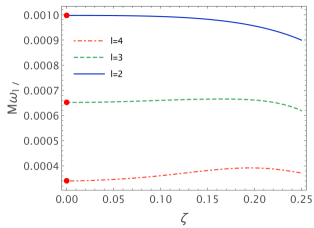
Figure 1: First-order rotational corrections $\omega_{1}$ (see Eq. (51)) of the gravitational QNMs with $n=0$ and $l=2,3,4$, as functions of the coupling parameter $\zeta$. The small circles are the values corresponing to Kerr BHs. The real parts are shown in the upper panel, the imaginary parts in the lower panel.

Estimate of the truncation errors

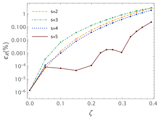
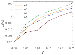
Figure 2: Relative discrepancy (Eq. (54)) between the estimate of $\omega_{1}$ for the $l=m=2$ fundamental mode computed to $O(\zeta^{s})$ and to $O(\zeta^{s+1})$, for different values of the coupling parameter $\zeta$.

In order to estimate the error in $\omega_{1}$ due to the truncation of the expansion in $\zeta$, we compare $\omega_{1}$ computed at $O(\zeta^{s})$ and at $O(\zeta^{s+1})$. In Fig. 2 we show the relative error

$$\epsilon^{s}_{R/I}=\frac{|\omega_{1\,R/I}^{(s+1)}-\omega_{1\,R/I}^{(s)}|}{\omega_{1\,R/I}^{(s)}}$$ (54)

(where the superscript $(s)$ denotes the order of $\zeta$ included in the perturbative expansion), for $s\leq 5$ and $\zeta\in[0,0.4]$ for the real part, $\zeta\in[0,0.25]$ for the imaginary part. This provides evidence that the truncation error due to the expansion in $\zeta$ is always $\lesssim 1\%$.

Conversely, it is impossible to provide a reliable estimate of the error due to the truncation at first order in the spin. Yet, the integration of the test scalar field (see Table 1) gives the indication that a first-order computation may provide the leading-order contribution of the modes (in particular of the real part). Generally speaking, corrections at order $O({\bar{a}}^{2})$ may be qualitatively different from those at order $O(\bar{a})$; there is no guarantee, then, that the latter dominate the QNM frequencies unless the spin is very low. Thus, our results should be considered as a first estimate of the rotational corrections to the QNMs in EdGB gravity.

Discussion of the results

In order to assess how rotation affects the EdGB corrections to the QNMs, in Figure 3 we show the ratio between the QNM frequency $\omega^{nlm}$ (for $n=0$, $l=m=2$) in EdGB gravity and in general relativity, for different values of $\zeta$. We only show the real part of the frequency, which we model as in Eq. (51).

We consider values of the spin $\bar{a}\in[0,0.7]$ (the latter corresponding to the typical outcome of a binary BH merger). As discussed above, since we neglect terms $O({\bar{a}}^{2})$, this model is accurate for $\bar{a}\ll 1$, while it should be only considered as an order-of-magnitude estimate of the corrections for $\bar{a}\lesssim 0.7$.

As shown in Fig. (3), rotation significantly magnifies the correction due to modified gravity. For $\zeta=0.4$, the mode is shifted of $\sim 4\%$ in a non-rotating BH, while the shift increases to $\sim 18\%$ for a BH with $\bar{a}=0.7$. This result may be due do the fact that rotating BHs have smaller horizon radii, and thus the curvature near the horizon is larger; this leads to larger effects in theories, like EdGB, in which the action contains terms quadratic in the curvature tensor.

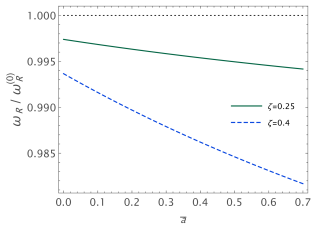
Figure 3: Ratio between the (real part of the) $n=0$, $l=m=2$ QNM frequency, computed up to $O(\bar{a})$, and the corresponding value in general relativity, as a function of the BH spin, for $\zeta=0.25$ and for $\zeta=0.4$.

IV Conclusions and outlook

In this article we have computed the QNMs of a rotating BH in EdGB gravity, a promising example of modified gravity theory in which the deviations of GR appear in the large-curvature regime. This is the first computation of QNMs of a rotating BH in modified gravity.

Although we have tested our approach up to order $O({\bar{a}}^{2})$ in the case of a test scalar field, the gravitational QNMs have only been computed to order $O(\bar{a})$. Thus, our results are accurate for $\bar{a}\ll 1$, while for larger values of the spin (as those typical in actual BHs formed in compact binary coalescences) they should be considered as an estimate of the actual QNM frequencies, and our calculation should be considered as the first step towards a reliable computation of the QNMs of rotating BHs in modified gravity theories, to be used in data-analysis frameworks such as TIGER [60] or ParSpec [61].

We compute the shifts of the frequencies due to rotation, $\omega_{1}$, as defined in Eq. (51). In Eqs. (52) we provide analytical fits of the real and imaginary parts of $\omega_{1}$, for the fundamental modes with $l=2,3$.

Our results suggest that the shifts of the frequencies due to general relativity modifications are magnified by rotation; for $\bar{a}\sim 0.7$, they can be larger than four times the corresponding shifts for a non-rotating BH.

The next step, presently in preparation [62], is the computation of the QNMs to second order in the spin. In this case, the couplings between perturbations with different values of the harmonic index $l$ can not be neglected (as in the case of the test scalar field, see Sec. III.4). Moreover, the gravitational perturbations are coupled with the scalar perturbation. Thus, both the derivation of the perturbation equations at $O({\bar{a}}^{2})$ and their numerical implementation are more involved.

Appendix A Equations for gravitational perturbations at first order in the spin

The field equations (3), (4), linearized in the perturbation around the stationary BH solution discussed in Sec. II, can be written as follows (we follow the same notation as [55], and leave implicit the sum over $l,m$):

$$\left[A^{(I)}_{lm}+\tilde{A}^{(I)}_{lm}\cos\theta\right]Y^{lm}(\theta)+imC^{(I)}_{lm}Y^{lm}(\theta)$$

$$+B^{(I)}_{lm}\sin\theta Y^{lm}_{,\theta}(\theta)=0\,,$$ (55)

$$\left[\alpha^{(J)}_{lm}+\tilde{\alpha}^{(J)}_{lm}\cos\theta\right]\sin\theta Y^{lm}_{,\theta}(\theta)-im\Big{[}\beta^{(J)}_{lm}$$

$$+\tilde{\beta}^{(J)}_{lm}\cos\theta\Big{]}Y^{lm}(\theta)+{\hat{\eta}}^{(J)}_{lm}\sin^{2}\theta Y^{lm}(\theta)$$

$$+{\hat{\xi}}^{(J)}_{lm}\sin\theta X^{lm}(\theta)+{\hat{\gamma}}^{(J)}_{lm}sin^{2}\theta W^{lm}(\theta)=0\,,$$ (56)

$$-\left[\beta^{(J)}_{lm}+\tilde{\beta}^{(J)}_{lm}\cos\theta\right]\sin\theta Y^{lm}_{,\theta}(\theta)-im\Big{[}\alpha^{(J)}_{lm}$$

$$+\tilde{\alpha}^{(J)}_{lm}\cos\theta\Big{]}Y^{lm}(\theta)-{\hat{\zeta}}^{(J)}_{lm}\sin^{2}\theta Y^{lm}(\theta)$$

$$-{\hat{\gamma}}^{(J)}_{lm}\sin\theta X^{lm}(\theta)+{\hat{\xi}}^{(J)}_{lm}\sin^{2}\theta W^{lm}(\theta)=0\,,$$ (57)

$$\ \hat{f}_{lm}\sin\theta Y^{lm}_{,\theta}(\theta)+im\hat{g}_{lm}Y^{lm}(\theta)+\hat{s}_{lm}\frac{X^{lm}(\theta)}{\sin\theta}$$

$$+\hat{t}_{lm}W^{lm}(\theta)=0\,,$$ (58)

$$\hat{g}_{lm}\sin\theta Y^{lm}_{,\theta}(\theta)-im\hat{f}_{lm}Y^{lm}(\theta)-\hat{t}_{lm}\frac{X^{lm}(\theta)}{\sin\theta}$$

$$+\hat{s}_{lm}W^{lm}(\theta)=0\,,$$ (59)

where in Eq. (55), $I=0,1,2,3$ correspond to the components of Einstein’s field equations behaving as scalars under rotations, and $I=4$ corresponds to the scalar field equation; $J=0,1$ in Eqs. (56), (57) correspond to the components of Einstein’s field equations behaving as vectors under rotations; and Eqs. (58), (59), correspond to the components of Einstein’s field equations behaving as tensors under rotations. We have defined

$$X^{lm}(\theta,\varphi)\equiv 2Y^{lm}_{,\theta\varphi}-2\frac{\cos\theta}{\sin\theta}Y^{lm}_{,\varphi}$$ (60)

$$W^{lm}(\theta,\varphi)\equiv-2\frac{\cos\theta}{\sin\theta}Y_{,\theta}-l(l+1)Y^{lm}-2\frac{Y^{lm}_{,\varphi\varphi}}{\sin^{2}\theta}\,.$$ (61)

The coefficients $A^{(I)}_{lm}$, $\alpha^{(J)}_{lm}$, $\beta^{(J)}_{lm}$, $\hat{s}_{lm}$, $\hat{t}_{lm}$ (of zero-th order in the spin) and ${\tilde{A}}^{(I)}_{lm}$, $C^{(I)}_{lm}$, $B^{(I)}_{lm}$, ${\tilde{\alpha}}^{(J)}_{lm}$, ${\tilde{\beta}}^{(J)}_{lm}$, ${\hat{\eta}}^{(J)}_{lm}$, ${\hat{\xi}}^{(J)}_{lm}$, ${\hat{\gamma}}^{(J)}_{lm}$, ${\hat{\zeta}}^{(J)}_{lm}$, $\hat{f}_{lm}$, $\hat{g}_{lm}$ (of order $O({\bar{a}})$) are linear combinations of the perturbation functions $h^{lm}_{0}(r)$, $h^{lm}_{1}(r)$, $H^{lm}_{0}(r)$, $H^{lm}_{1}(r)$, $H^{lm}_{2}(r)$, $K^{lm}(r)$, $\Phi^{lm}(r)$ and their derivatives, with coefficients that depend on $l$ but not on $m$. Their explicit espansions in the coupling parameter $\zeta$, up to $O(\zeta^{6})$, are given in the supplemental Mathematica notebook [54].

We project Eqs. (55) - (59) on the complete set of tensor spherical harmonics, as in [55], finding the decoupled equations:

$$A^{(I)}_{{l}m}+imC^{(I)}_{{l}m}+Q_{l}\left[\tilde{A}^{(I)}_{{l}-1\,m}+({l}-1)B^{(I)}_{{l}-1\,m}\right]$$

$$+Q_{{l}+1\,m}\left[\tilde{A}^{(I)}_{{l}+1\,m}-({l}+2)B^{(I)}_{{l}+1\,m}\right]=0$$ (62)

$${l}({l}+1)\alpha^{(J)}_{{l}m}-im\left[\tilde{\beta}^{(J)}_{{l}m}+{\hat{\zeta}}^{(J)}_{{l}m}-({l}-1)({l}+2){\hat{\xi}}^{(J)}_{{lm}}\right]$$

$$+Q_{{l}m}({l}+1)\left[({l}-1)\tilde{\alpha}^{(J)}_{{l}-1\,m}-{\hat{\eta}}^{(J)}_{{l}-1\,m}+({l}-2)({l}-1){\hat{\gamma}}^{(J)}_{{l}-1\,m}\right]$$

$$+Q_{{l}+1}{l}\left[({l}+2)\tilde{\alpha}^{(J)}_{{l}+1\,m}+{\hat{\eta}}^{(J)}_{{l}+1\,m}-({l}+2)({l}+3){\hat{\gamma}}^{(J)}_{{l}+1\,m}\right]=0$$ (63)

$${l}({l}+1)\beta^{(J)}_{{l}m}+im\left[\tilde{\alpha}^{(J)}_{{l}m}+{\hat{\eta}}^{(J)}_{{l}m}+({l}-1)({l}+2){\hat{\gamma}}^{(J)}_{{l}}\right]$$

$$+Q_{{l}m}({l}+1)\left[({l}-1)\tilde{\beta}^{(J)}_{{l}-1\,m}-{\hat{\zeta}}^{(J)}_{{l}-1\,m}-({l}-2)({l}-1){\hat{\xi}}^{(J)}_{{l}-1}\right]$$

$$+Q_{{l}+1\,m}{l}\left[({l}+2)\tilde{\beta}^{(J)}_{{l}+1\,m}+{\hat{\zeta}}^{(J)}_{{l}+1\,m}+({l}+2)({l}+3){\hat{\xi}}^{(J)}_{{l}+1}\right]=0$$ (64)

$${l}({l}-1)({l}+1)({l}+2)\hat{s}_{lm}-im({l}-1)({l}+2)\hat{f}_{lm}$$

$$-Q_{{lm}}({l}-1)({l}+1)({l}+2)\hat{g}_{{l}-1\,m}$$

$$+Q_{{l}+1}{l}({l}-1)({l}+2)\hat{g}_{{l}+1\,m}=0$$ (65)

$${l}({l}-1)({l}+1)({l}+2)\hat{t}_{lm}+im({l}-1)({l}+2)\hat{g}_{lm}$$

$$-Q_{{l}m}({l}-1)({l}+1)({l}+2)\hat{f}_{{l}-1\,m}$$

$$+Q_{{l}+1\,m}{l}({l}-1)({l}+2)\hat{f}_{{l}+1\,m}=0\,,$$ (66)

where $l\geq 2$ and

$$Q_{lm}=\sqrt{\frac{(l-m)(l+m)}{(2l-1)(2l+1)}}\,.$$ (67)

As discussed in Sec. III.5, the QNMs at order $O({\bar{a}})$ are not affected by the coupling terms, which can then be neglected. Thus, Eqs. (62) - (66) reduce to Eqs. (46).

Appendix B Tortoise coordinate for stationary black holes in Einstein-dilaton Gauss-Bonnet gravity

The tortoise coordinate $r_{*}$ is a redefinition of the radial coordinate $r$, mapping the region outside the BH horizon $r\in[r_{\rm h},+\infty]$ into $r_{*}\in[-\infty,+\infty]$. By defining

$$\frac{dr}{dr_{*}}=F(r)$$ (68)

the function $F(r)$, safisfying $F(r)\sim r-r_{\rm h}$ for $r\to r_{\rm h}$ and $F(r)\to 1$ for $r\to\infty$, can be found by requiring that the perturbation equations reduce, at the horizon and at infinity, to Eq. (22). In general relativity, $F(r)=1-2M/r$ for Schwarzschild BHs, and $F(r)=(r^{2}+a^{2}-2Mr)/(r^{2}+a^{2})\sim(r-r_{\rm h})$ (where $r_{\rm h}=2M-a^{2}/(2M)+O(a^{4})$) for Kerr BHs. We shall define the tortoise coordinate in EdGB gravity, by requiring the equation for a test scalar field to have the form (22). We have verified (up to first order in the spin) that this coordinate defines the boundary conditions for the gravitational perturbations as well; this is expected, since the null ingoing coordinate $v=t+r_{*}$ (with a similar redefinition of the azimuthal coordinate $\varphi$) should regularize the coordinate singularity at the horizon, and thus the tortoise coordinate has to be the same for scalar and gravitational perturbations.

Non-rotating BHs

The metric of a static BH in EdGB gravity is Eq. (6),

$$ds^{2}=-A(r)dt^{2}+\frac{dr^{2}}{B(r)}+r^{2}d\Omega^{2}\,.$$ (69)

The Klein-Gordon equation for a test scalar field, $\nabla_{\mu}\nabla^{\mu}\phi=0$, by expanding $\phi=\frac{1}{r}\phi^{lm}(r)Y^{lm}(\theta,\varphi)e^{-i\omega t}$, reads (we denote with a prime differentiation with respect to $r$):

$$AB\phi^{lm\prime\prime}+\frac{1}{2}(A^{\prime}B+B^{\prime}A)\phi^{lm\prime}$$

$$+\left(\omega^{2}-\frac{A^{\prime}B+B^{\prime}A}{2r}-A\frac{l(l+1)}{r^{2}}\right)\phi^{lm}=0\,.$$ (70)

By defining the tortoise coordinate with $F(r)=\sqrt{A(r)B(r)}$ [23], Eq. (70) can be written as

$$\phi^{lm}_{,r_{*}r_{*}}+(\omega^{2}-V^{l})\phi^{lm}=0$$ (71)

where $V^{l}=FF^{\prime}-Al(l+1)/r^{2}$, vanishing both at the horizon and at infinity (since $F^{\prime}\sim r^{-2}$). Since, for a non-rotating BH, $k_{\rm H}=\omega$, Eq. (71) coincides with Eq. (22).

First order in the spin

At $O(\bar{a})$, the metric (69) acquires the extra term $g_{t\varphi}=-r^{2}\sin^{2}\theta\varpi(r)$, where

$$\varpi(r)=\frac{2J}{r^{3}}\left[1-\frac{147}{960}\zeta^{2}\left(1+O\left(\frac{M}{r}\right)\right)+O(\zeta^{3})\right]\,.$$ (72)

Since $g_{\varphi\varphi}=r^{2}\sin^{2}\theta$,

$$\Omega_{\rm H}=-\lim_{r\to r_{\rm h}}\frac{g_{t\varphi}}{g_{\varphi\varphi}}=\varpi(r_{\rm h})\,.$$ (73)

The equation for a test scalar field in this spacetime acquires the extra term $-2m\omega\varpi(r)$. Then, by defining the tortoise coordinate as in the non-rotating case $F(r)=\sqrt{A(r)B(r)}$, the scalar field equation near the horizon (neglecting $O({\bar{a}}^{2})$ terms) reads:

$$\phi^{lm}_{,r_{*}r_{*}}+(\omega^{2}-2m\Omega_{\rm H}\omega)\phi^{lm}=\phi^{lm}_{,r_{*}r_{*}}+k_{\rm H}^{2}\phi^{lm}=0$$ (74)

in agreement with Eq. (22).

Second order in the spin

To define the tortoise coordinate we write $F(r)$ as a generic expansion in powers of $\zeta$, ${\bar{a}}$ and $\frac{1}{r}$, such that $F\sim r-r_{\rm h}$ near the horizon and $F(r)\to 1$ as $r\to\infty$. By requiring that the equation for a test scalar field has the form (22) near the horizon and near infinity, we find

$$F(r)= \left(1-\frac{r_{\rm h}}{r}\right)\left\{1-{\bar{a}}^{2}\frac{r_{\rm h}(r^{2}+rr_{\rm h}+r_{\rm h}^{2})}{8r^{3}}\right.$$

$$\left.-\zeta^{2}\left[\frac{r_{\rm h}}{3840r^{4}}(147r^{3}+117r^{2}r_{\rm h}-526rr_{\rm h}^{2}+263r_{\rm h}^{3})\right.\right.$$

$$\left.\left.+{\bar{a}}^{2}\frac{r_{\rm h}}{30720r^{3}}(375r^{2}+435rr_{\rm h}+343r_{\rm h}^{2})\right]\right\}$$

$$+O(\zeta^{3})+O({\bar{a}}^{3})\,.$$ (75)

In order to obtain this expression we imposed a condition sligthly stronger than Eq. (22): we required that at $r\to\infty$

$$Z^{lm}_{,r_{*}r_{*}}+\omega^{2}Z^{lm}=\frac{l(l+1)}{r^{2}}Z^{lm}+O\left(\frac{1}{r^{3}}\right)\,.$$

With this further condition, we obtained a better agreement with the results of [47] for the QNMs of a test scalar field.

References

- [1] LIGO Scientific, Virgo Collaboration, B. P. Abbott et al., “Observation of Gravitational Waves from a Binary Black Hole Merger,” Phys. Rev. Lett. 116 no. 6, (2016) 061102, arXiv:1602.03837 [gr-qc].
- [2] LIGO Scientific, Virgo Collaboration, B. P. Abbott et al., “Tests of general relativity with GW150914,” Phys. Rev. Lett. 116 no. 22, (2016) 221101, arXiv:1602.03841 [gr-qc]. [Erratum: Phys.Rev.Lett. 121, 129902 (2018)].
- [3] E. Barausse, N. Yunes, and K. Chamberlain, “Theory-Agnostic Constraints on Black-Hole Dipole Radiation with Multiband Gravitational-Wave Astrophysics,” Phys. Rev. Lett. 116 no. 24, (2016) 241104, arXiv:1603.04075 [gr-qc].
- [4] N. Yunes, K. Yagi, and F. Pretorius, “Theoretical Physics Implications of the Binary Black-Hole Mergers GW150914 and GW151226,” Phys. Rev. D 94 no. 8, (2016) 084002, arXiv:1603.08955 [gr-qc].
- [5] T. Delsate, D. Hilditch, and H. Witek, “Initial value formulation of dynamical Chern-Simons gravity,” Phys. Rev. D 91 no. 2, (2015) 024027, arXiv:1407.6727 [gr-qc].
- [6] G. Papallo and H. S. Reall, “On the local well-posedness of Lovelock and Horndeski theories,” Phys. Rev. D 96 no. 4, (2017) 044019, arXiv:1705.04370 [gr-qc].
- [7] J. L. Ripley and F. Pretorius, “Gravitational collapse in Einstein dilaton-Gauss–Bonnet gravity,” Class. Quant. Grav. 36 no. 13, (2019) 134001, arXiv:1903.07543 [gr-qc].
- [8] A. D. Kovács and H. S. Reall, “Well-posed formulation of Lovelock and Horndeski theories,” Phys. Rev. D 101 no. 12, (2020) 124003, arXiv:2003.08398 [gr-qc].
- [9] H. Witek, L. Gualtieri, and P. Pani, “Towards numerical relativity in scalar Gauss-Bonnet gravity: decomposition beyond the small-coupling limit,” Phys. Rev. D 101 no. 12, (2020) 124055, arXiv:2004.00009 [gr-qc].
- [10] F.-L. Julié and E. Berti, “ formalism in Einstein-scalar-Gauss-Bonnet gravity,” Phys. Rev. D 101 no. 12, (2020) 124045, arXiv:2004.00003 [gr-qc].
- [11] W. E. East and J. L. Ripley, “Evolution of Einstein-scalar-Gauss-Bonnet gravity using a modified harmonic formulation,” Phys. Rev. D 103 no. 4, (2021) 044040, arXiv:2011.03547 [gr-qc].
- [12] K. D. Kokkotas and B. G. Schmidt, “Quasinormal modes of stars and black holes,” Living Rev. Rel. 2 (1999) 2, arXiv:gr-qc/9909058.
- [13] V. Ferrari and L. Gualtieri, “Quasi-Normal Modes and Gravitational Wave Astronomy,” Gen. Rel. Grav. 40 (2008) 945–970, arXiv:0709.0657 [gr-qc].
- [14] E. Berti, V. Cardoso, and A. O. Starinets, “Quasinormal modes of black holes and black branes,” Class. Quant. Grav. 26 (2009) 163001, arXiv:0905.2975 [gr-qc].
- [15] O. Dreyer, B. J. Kelly, B. Krishnan, L. S. Finn, D. Garrison, and R. Lopez-Aleman, “Black hole spectroscopy: Testing general relativity through gravitational wave observations,” Class. Quant. Grav. 21 (2004) 787–804, arXiv:gr-qc/0309007.
- [16] E. Berti, V. Cardoso, and C. M. Will, “On gravitational-wave spectroscopy of massive black holes with the space interferometer LISA,” Phys. Rev. D 73 (2006) 064030, arXiv:gr-qc/0512160.
- [17] E. Berti, J. Cardoso, V. Cardoso, and M. Cavaglia, “Matched-filtering and parameter estimation of ringdown waveforms,” Phys. Rev. D 76 (2007) 104044, arXiv:0707.1202 [gr-qc].
- [18] E. Berti, K. Yagi, H. Yang, and N. Yunes, “Extreme Gravity Tests with Gravitational Waves from Compact Binary Coalescences: (II) Ringdown,” Gen. Rel. Grav. 50 no. 5, (2018) 49, arXiv:1801.03587 [gr-qc].
- [19] V. Cardoso and L. Gualtieri, “Perturbations of Schwarzschild black holes in Dynamical Chern-Simons modified gravity,” Phys. Rev. D 80 (2009) 064008, arXiv:0907.5008 [gr-qc]. [Erratum: Phys.Rev.D 81, 089903 (2010)].
- [20] C. Molina, P. Pani, V. Cardoso, and L. Gualtieri, “Gravitational signature of Schwarzschild black holes in dynamical Chern-Simons gravity,” Phys. Rev. D 81 (2010) 124021, arXiv:1004.4007 [gr-qc].
- [21] T. Kobayashi, H. Motohashi, and T. Suyama, “Black hole perturbation in the most general scalar-tensor theory with second-order field equations I: the odd-parity sector,” Phys. Rev. D 85 (2012) 084025, arXiv:1202.4893 [gr-qc]. [Erratum: Phys.Rev.D 96, 109903 (2017)].
- [22] T. Kobayashi, H. Motohashi, and T. Suyama, “Black hole perturbation in the most general scalar-tensor theory with second-order field equations II: the even-parity sector,” Phys. Rev. D 89 no. 8, (2014) 084042, arXiv:1402.6740 [gr-qc].
- [23] J. L. Blázquez-Salcedo, C. F. B. Macedo, V. Cardoso, V. Ferrari, L. Gualtieri, F. S. Khoo, J. Kunz, and P. Pani, “Perturbed black holes in einstein-dilaton-gauss-bonnet gravity: Stability, ringdown, and gravitational-wave emission,” Phys. Rev. D 94 (Nov, 2016) 104024. https://link.aps.org/doi/10.1103/PhysRevD.94.104024.
- [24] O. J. Tattersall, “Quasi-Normal Modes of Hairy Scalar Tensor Black Holes: Odd Parity,” Class. Quant. Grav. 37 no. 11, (2020) 115007, arXiv:1911.07593 [gr-qc].
- [25] J. L. Blázquez-Salcedo, D. D. Doneva, S. Kahlen, J. Kunz, P. Nedkova, and S. S. Yazadjiev, “Polar quasinormal modes of the scalarized Einstein-Gauss-Bonnet black holes,” Phys. Rev. D 102 no. 2, (2020) 024086, arXiv:2006.06006 [gr-qc].
- [26] J. L. Blázquez-Salcedo, F. S. Khoo, and J. Kunz, “Quasinormal modes of Einstein-Gauss-Bonnet-dilaton black holes,” Phys. Rev. D 96 no. 6, (2017) 064008, arXiv:1706.03262 [gr-qc].
- [27] V. Cardoso, M. Kimura, A. Maselli, E. Berti, C. F. B. Macedo, and R. McManus, “Parametrized black hole quasinormal ringdown: Decoupled equations for nonrotating black holes,” Phys. Rev. D 99 no. 10, (2019) 104077, arXiv:1901.01265 [gr-qc].
- [28] R. McManus, E. Berti, C. F. B. Macedo, M. Kimura, A. Maselli, and V. Cardoso, “Parametrized black hole quasinormal ringdown. II. Coupled equations and quadratic corrections for nonrotating black holes,” Phys. Rev. D 100 no. 4, (2019) 044061, arXiv:1906.05155 [gr-qc].
- [29] E. Berti et al., “Testing General Relativity with Present and Future Astrophysical Observations,” Class. Quant. Grav. 32 (2015) 243001.
- [30] J. Antoniadis et al., “A Massive Pulsar in a Compact Relativistic Binary,” Science 340 (2013) 6131, arXiv:1304.6875 [astro-ph.HE].
- [31] S. Mignemi and N. R. Stewart, “Charged black holes in effective string theory,” Phys. Rev. D 47 (1993) 5259–5269, arXiv:hep-th/9212146.
- [32] P. Kanti, N. E. Mavromatos, J. Rizos, K. Tamvakis, and E. Winstanley, “Dilatonic black holes in higher curvature string gravity,” Phys. Rev. D54 (1996) 5049–5058.
- [33] G. W. Horndeski, “Second-order scalar-tensor field equations in a four-dimensional space,” Int. J. Theor. Phys. 10 (1974) 363–384.
- [34] T. Kobayashi, “Horndeski theory and beyond: a review,” Rept. Prog. Phys. 82 no. 8, (2019) 086901, arXiv:1901.07183 [gr-qc].
- [35] G. Carullo, “Accelerating modified gravity detection from gravitational-wave observations using the Parametrized ringdown spin expansion coefficients formalism,” arXiv:2102.05939 [gr-qc].
- [36] K. Yagi, “A New constraint on scalar Gauss-Bonnet gravity and a possible explanation for the excess of the orbital decay rate in a low-mass X-ray binary,” Phys. Rev. D 86 (2012) 081504, arXiv:1204.4524 [gr-qc].
- [37] B. C. Seymour and K. Yagi, “Testing General Relativity with Black Hole-Pulsar Binaries,” Phys. Rev. D 98 no. 12, (2018) 124007, arXiv:1808.00080 [gr-qc].
- [38] H. Witek, L. Gualtieri, P. Pani, and T. P. Sotiriou, “Black holes and binary mergers in scalar Gauss-Bonnet gravity: scalar field dynamics,” Phys. Rev. D 99 no. 6, (2019) 064035, arXiv:1810.05177 [gr-qc].
- [39] V. Ferrari and B. Mashhoon, “New approach to the quasinormal modes of a black hole,” Phys. Rev. D 30 (1984) 295–304.
- [40] V. Cardoso, A. S. Miranda, E. Berti, H. Witek, and V. T. Zanchin, “Geodesic stability, Lyapunov exponents and quasinormal modes,” Phys. Rev. D 79 (2009) 064016, arXiv:0812.1806 [hep-th].
- [41] H. Yang, D. A. Nichols, F. Zhang, A. Zimmerman, Z. Zhang, and Y. Chen, “Quasinormal-mode spectrum of Kerr black holes and its geometric interpretation,” Phys. Rev. D 86 (2012) 104006, arXiv:1207.4253 [gr-qc].
- [42] S. Alexander and N. Yunes, “Chern-Simons Modified General Relativity,” Phys. Rept. 480 (2009) 1–55, arXiv:0907.2562 [hep-th].
- [43] F. Moura and J. a. Rodrigues, “Eikonal quasinormal modes and shadow of string-corrected -dimensional black holes,” arXiv:2103.09302 [hep-th].
- [44] J. B. Hartle and K. S. Thorne, “Slowly Rotating Relativistic Stars. II. Models for Neutron Stars and Supermassive Stars,” Astrophys. J. 153 (1968) 807.
- [45] P. Pani, V. Cardoso, L. Gualtieri, E. Berti, and A. Ishibashi, “Perturbations of slowly rotating black holes: massive vector fields in the Kerr metric,” Phys. Rev. D 86 (2012) 104017, arXiv:1209.0773 [gr-qc].
- [46] P. Pani, E. Berti, and L. Gualtieri, “Gravitoelectromagnetic Perturbations of Kerr-Newman Black Holes: Stability and Isospectrality in the Slow-Rotation Limit,” Phys. Rev. Lett. 110 no. 24, (2013) 241103, arXiv:1304.1160 [gr-qc].
- [47] P. A. Cano, K. Fransen, and T. Hertog, “Ringing of rotating black holes in higher-derivative gravity,” Phys. Rev. D 102 no. 4, (2020) 044047, arXiv:2005.03671 [gr-qc].
- [48] P. Pani and V. Cardoso, “Are black holes in alternative theories serious astrophysical candidates? The Case for Einstein-Dilaton-Gauss-Bonnet black holes,” Phys. Rev. D79 (2009) 084031.
- [49] T. P. Sotiriou and S.-Y. Zhou, “Black hole hair in generalized scalar-tensor gravity: An explicit example,” Phys. Rev. D 90 (2014) 124063, arXiv:1408.1698 [gr-qc].
- [50] B. Kleihaus, J. Kunz, S. Mojica, and E. Radu, “Spinning black holes in Einstein–Gauss-Bonnet–dilaton theory: Nonperturbative solutions,” Phys. Rev. D 93 no. 4, (2016) 044047, arXiv:1511.05513 [gr-qc].
- [51] N. Yunes and L. C. Stein, “Non-Spinning Black Holes in Alternative Theories of Gravity,” Phys. Rev. D 83 (2011) 104002, arXiv:1101.2921 [gr-qc].
- [52] B. Kleihaus, J. Kunz, and E. Radu, “Rotating Black Holes in Dilatonic Einstein-Gauss-Bonnet Theory,” Phys. Rev. Lett. 106 (2011) 151104, arXiv:1101.2868 [gr-qc].
- [53] A. Maselli, P. Pani, L. Gualtieri, and V. Ferrari, “Rotating black holes in Einstein-Dilaton-Gauss-Bonnet gravity with finite coupling,” Phys. Rev. D 92 no. 8, (2015) 083014.
- [54] https://web.uniroma1.it/gmunu/resources/.
- [55] Y. Kojima, “Equations governing the nonradial oscillations of a slowly rotating relativistic star,” Phys. Rev. D46 (1992) 4289–4303.
- [56] P. Pani, “Advanced Methods in Black-Hole Perturbation Theory,” Int. J. Mod. Phys. A 28 (2013) 1340018, arXiv:1305.6759 [gr-qc].
- [57] Y. Kojima, “Coupled Pulsations between Polar and Axial Modes in a Slowly Rotating Relativistic Star,” Progress of Theoretical Physics 90 no. 5, (Nov., 1993) 977–990.
- [58] Y. Kojima, “Normal Modes of Relativistic Stars in Slow Rotation Limit,” ApJ 414 (Sept., 1993) 247.
- [59] https://pages.jh.edu/eberti2/ringdown/.
- [60] J. Meidam, M. Agathos, C. Van Den Broeck, J. Veitch, and B. S. Sathyaprakash, “Testing the no-hair theorem with black hole ringdowns using TIGER,” Phys. Rev. D 90 no. 6, (2014) 064009, arXiv:1406.3201 [gr-qc].
- [61] A. Maselli, P. Pani, L. Gualtieri, and E. Berti, “Parametrized ringdown spin expansion coefficients: a data-analysis framework for black-hole spectroscopy with multiple events,” Phys. Rev. D 101 no. 2, (2020) 024043, arXiv:1910.12893 [gr-qc].
- [62] R. McManus, L. Pierini, et al. in preparation.