Black hole evaporation in de Sitter space

Abstract

We investigate the evaporation process of a Kerr-de Sitter black hole with the Unruh-Hawking-like vacuum state, which is a realistic vacuum state modelling the evaporation process of a black hole originating from gravitational collapse. We also compute the greybody factors for gravitons, photons, and conformal-coupling massless scalar particles by using the analytic solutions of the Teukolsky equation in the Kerr-de Sitter background. It turns out that the cosmological constant quenches the amplification factor and it approaches to zero towards the critical point where the Nariai and extremal limits merge together. We confirm that even near the critical point, the superradiance of gravitons is more significant than that of photons and scalar particles. Angular momentum is carried out by particles several times faster than the mass energy decreases. This means that a Kerr-de Sitter black hole rapidly spins down to a nearly Schwarzschild-de Sitter black hole before it completely evaporates. We also compute the time evolution of the Bekenstein-Hawking entropy. The total entropy of the Kerr-de Sitter black hole and cosmological horizon increases with time, which is consistent with the generalized second law of thermodynamics.

1 Introduction

The theory of black hole evaporation stands as something of a milestone in theoretical physics. In the context of quantum field theory on a curved spacetime background, black holes radiate thermal radiation, modified by scattering effects from the spacetime geometry. The backreaction of the radiation flux causes the black hole to evaporate, and black holes are expected to lose all their mass and angular momentum. In this paper we address the fate of a black hole in de Sitter space, where the black hole and the surrounding spacetime have potentially different temperatures. We focus on the situation where the black hole and the de Sitter space both have a finite past history, such as might arise in the early universe with black holes that form from gravitational collapse.

The evolution of mass and angular momentum for black holes in empty space was first discussed in the pioneering papers of Hawking Hawking (1974, 1975), where it was proposed that the black hole loses mass at an increasing rate until nothing is left. The numerical details were supplied by Page Page (1976a) and extended to rotating holes a little later Page (1976b). Page found that the black hole always loses angular momentum more rapidly than it loses mass. The backreaction of radiation emitted by the black hole can also be studied directly via the quantum expectation value of the stress-energy tensor Candelas (1980), and there has been recent progress calculating the full quantum stress tensor Levi and Ori (2015); Levi (2017); Levi et al. (2017).

The evolution of mass and angular momentum are related to the fluxes of energy and angular momentum from quantum fields around the black hole. These fluxes are expectation values, or ensemble averaged expectation values, of a quantum stress tensor $\hat{T}_{\mu\nu}$ Candelas (1980). The choice of quantum states plays a crucial role in evaluating these expectation values. We illustrate this by reviewing what happens for an eternal black hole background in an asymptotically flat spacetime.

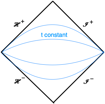
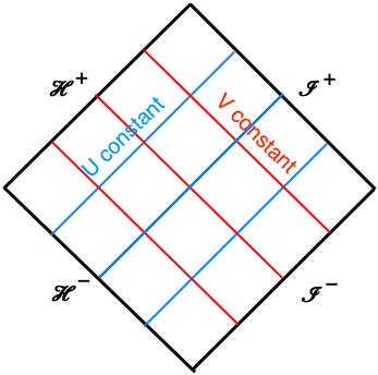
Figure 1: Penrose diagram for the exterior of a black hole in asymptotically flat spacetime.

Three quantum vacuum states play significant roles Unruh (1976). Each is defined with respect to sets of positive frequency wave modes on the background spacetime:

• the Boulware vacuum $|B\rangle$, defined by taking modes which are positive frequency with respect to the Killing vector $\partial_{t}$, with respect to which the exterior region is static,

• the Unruh-Hawking vacuum $|U\rangle$, defined by taking modes that are incoming from $\mathscr{I}^{-}$ to be positive frequency with respect to $\partial_{t}$, while those that emanate from the past horizon are taken to be positive frequency with respect to $\partial_{U}$, where $U$ is the canonical affine parameter on the past horizon,

• the Hartle-Hawking vacuum $|H\rangle$, defined by taking incoming modes to be positive frequency with respect to $\partial_{V}$, where $V$ is the canonical affine parameter on the future horizon, and outgoing modes to be positive frequency with respect to $\partial_{U}$.

The vacuum state is said to be regular on the horizon if the Feynman two-point function for that vacuum state is regular there. In practice, this means that the first derivative of the Feynman Green function with respect to the Kruskal coordinates is finite. The Boulware vacuum state is not regular on either the past or future black hole horizons, which nevertheless makes it suitable for the space outside a neutron star, for example, where the spacetime is locally isometric to the black hole metric but neither horizon is present.

The Unruh-Hawking vacuum state is used for a black hole formed from gravitational collapse. In reality, the collapse would result in a highly excited state. However, the no hair theorems imply that the initial excitations would rapidly decay away and the state would be expected to evolve to the vacuum state over a short period of time. Despite being a vacuum state, the particle flux from the hole is non-vanishing, and has a thermal spectrum at the Hawking temperature modified by particle scattering from the spacetime geometry, and super-radiance contributions if the black hole is rotating.

The affine parameter $U$, shown on the right in figure 1, vanishes at the future black hole horizon. The Unruh-Hawking vacuum state is regular on $U=0$. The state is not regular on the past black hole event horizon, where the derivative of the Green’s functions with respect to $V$ diverges.

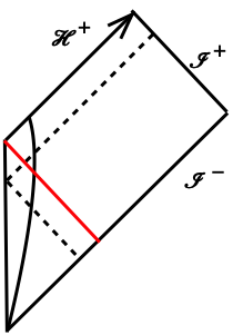
Figure 2: Penrose diagram for a collapsing star.

The past horizon is not present in the typical collapse situation shown in figure 2. Instead, there is a null surface spanned by infalling null rays converging on the point where the future event horizon forms. We can think of this surface as a virtual past horizon. In the geometrical optics limit, wave vectors follow the paths of null geodesics. Hence, high-frequency infalling waves with wave vector $\partial_{v}$, that pass through the the collapsing star, emerge as outgoing waves with wave vector $\partial_{V}$. This converts a fraction of the positive frequency $\partial_{t}$ modes into outgoing positive frequency $\partial_{V}$ modes.

The Hartle-Hawking vacuum is used for the ‘black hole in box’, to represent a thermodynamical ensemble at the Hawking temperature. The vacuum state is regular on both the past and future black hole horizons, and particle fluxes are in perfect balance. However, gravitational backreaction from the Hawking radiation is not consistent with having an asymptotically flat spacetime, hence the need for a reflecting barrier around the hole to cut off the radiation.

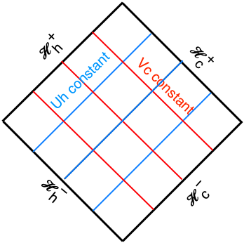
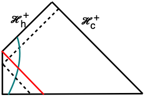
Figure 3: Penrose diagrams for the exterior region of an eternal black hole in de Sitter space and a collapsing region in de Sitter space starting from a spacelike surface. The affine parameter $U_{h}=-e^{-\kappa_{h}u}$ is zero on the future black hole horizon ${\cal H}_{h}^{+}$, and $V_{c}=-e^{-\kappa_{c}v}$ is zero on the future cosmological horizon ${\cal H}_{c}^{+}$.

We turn now to the black hole in de Sitter space. The cosmological horizon of de Sitter space emits particles with temperature $T_{c}$ Gibbons and Hawking (1977) which is typically different from the black hole temperature $T_{h}$. There are two particle fluxes in competition, an incoming flux from the cosmological horizon and an outgoing flux from the black hole. To represent this situation we generalise the Unruh-Hawking vacuum state as follows:

The vacuum state $|V\rangle$ is defined by taking modes that are incoming from the past cosmological horizon to be positive frequency with respect to $\partial_{V_{c}}$, while those that emanate from the past black hole horizon are taken to be positive frequency with respect to $\partial_{U_{h}}$, the canonical affine parameter on the past horizon.

A similar vacuum state has been used to analyse particle production from non-rotating black holes in de Sitter space in Qiu and Traschen (2020); Anderson and Traschen (2020). Note that the state is not the ‘Unruh’ state used for de Sitter space in Aalsma, Parikh, and Van Der Schaar (2019); Gong and Seo (2020), where the authors use ingoing modes for $\partial_{U_{c}}$ and outgoing for $\partial_{t}$.

The same argument given in Ref Unruh (1976) implies that this vacuum state is regular on the future black hole horizon, where the parameter $U_{h}$ vanishes, and on the future cosmological horizon, where the parameter $V_{c}$ vanishes. We cannot say for sure that this is the unique vacuum state with this property, in the sense that there is a unique vacuum state which is regular on the future and past black hole horizons in asymptotically flat space Kay and Wald (1991).

Consider next how the state could emerge physically. Globally, de Sitter space represents a universe that collapses from the infinite past, bounces and then expands to the infinite future. In a big bang cosmology, de Sitter space arises locally as part of the inflationary universe scenario. The collapse phase is absent, as is the past cosmological horizon. However, the initial quantum state of the inflationary universe is usually taken to be the Bunch-Davies vacuum state Bunch and Davies (1978), which is positive frequency with respect to the de Sitter killing vectors $\partial_{U_{c}}$ and $\partial_{V_{c}}$. Now suppose a black hole forms. In the geometrical optics limit, ingoing waves with wave vector $\partial_{V_{c}}$ that pass through the collapsing body are converted into outgoing waves with wave vector $\partial_{U_{h}}$, as shown in the Penrose diagram on the right of figure 3. A fraction of the incoming modes should therefore become positive frequency $\partial_{U_{h}}$ modes.

As in the asymptotically flat case, we expect the excited quantum state to settle down to the vacuum state at late (advanced) time. This occurs in the classical theory, where it has been shown that the no hair theorem extends to black holes in de Sitter space Mellor and Moss (1990); Chambers and Moss (1994a). The decay rate of perturbations is exponential at late cosmological time Chambers and Moss (1994a). The outgoing waves with wave vector $\partial_{U_{c}}$ that are present in the initial state should also decay away, leaving the positive frequency $\partial_{U_{h}}$ modes.

Given the vacuum state $|V\rangle$, the evolution of the mass $M$ and angular momentum $J$ of the black hole in de Sitter space with cosmological constant $3/\ell^{2}$ are governed by the energy and angular momentum fluxes $\langle V|\hat{T}_{rt}|V\rangle$ and $\langle V|\hat{T}_{r\varphi}|V\rangle$. These will be calculated in section 3 from the appropriate mode decompositions of scalar quantum fields. We will arrive at pleasingly compact results for a black hole in de Sitter space,

$${dM\over dt} =-\sum_{lm_{z}}\int_{0}^{\infty}{d\omega\over 2\pi}\left(\omega-{J\over M\ell^{2}}m_{z}\right)\left(1-|A_{\omega lm_{z}}|^{2}\right)\frac{1}{2}\left\{{\rm coth}{\beta_{h}\omega_{h}\over 2}-{\rm coth}{\beta_{c}\omega_{c}\over 2}\right\},$$ (1)

$${dJ\over dt} =-\sum_{lm_{z}}\int_{0}^{\infty}{d\omega\over 2\pi}\,m_{z}\left(1-|A_{\omega lm_{z}}|^{2}\right)\frac{1}{2}\left\{{\rm coth}{\beta_{h}\omega_{h}\over 2}-{\rm coth}{\beta_{c}\omega_{c}\over 2}\right\},$$ (2)

where $\beta_{i}$ are inverse temperatures at the black hole ($i=h$) and cosmological ($i=c$) horizons, respectively. The horizon frequencies $\omega_{i}\equiv\omega-m_{z}\Omega_{i}$ in terms of the horizon rotation $\Omega_{i}$, and the factors $A_{\omega lm_{z}}$ are reflection coefficients for waves transiting the spacetime geometry. Finally, $l$ and $m_{z}$ are the angular and azimuthal modes, respectively. One should be careful not to confuse the angular mode $l$ with the de Sitter radius $\ell$.

Special cases include:

• The Boulware vacuum $\beta_{h}\to\infty$, $\beta_{c}\to\infty$,

  $${dM\over dt}=\sum_{lm_{z}}\int_{\omega_{c}\omega_{h}<0}{d\omega\over 4\pi}|\omega|\left(1-|A_{\omega lm_{z}}|^{2}\right),$$ (3)

  in agreement with Unruh, Unruh (1974).

• The Unruh-Hawking vacuum (non-rotating case) $\beta_{c}\to\infty$, $\omega_{h}=\omega_{c}=\omega$,

  $${dM\over dt}=-\sum_{lm_{z}}\int_{0}^{\infty}{d\omega\over 2\pi}\omega\left(1-|A_{\omega lm_{z}}|^{2}\right){1\over e^{\beta_{h}\omega}-1},$$ (4)

  as originally derived by Hawking Hawking (1975).

• The Unruh-Hawking vacuum (rotating case) $\beta_{c}\to\infty$, $\omega_{c}=\omega$

  $${dM\over dt}=-\sum_{lm_{z}}\int_{0}^{\infty}{d\omega\over 2\pi}\omega\left(1-|A_{\omega lm_{z}}|^{2}\right){1\over e^{\beta_{h}\omega_{h}}-1}.$$ (5)

  which was also derived by Hawking Hawking (1975).

Note that the fluxes diverge in the $M\to 0$ or $\Lambda\to\infty$ limits, so the formulae don’t apply to the case $M=0$.

The evolution of mass and angular momentum is described in detail in §4. The most difficult part of the calculation is evaluating the reflection and transmissions factors. We have evaluated these for the combinations of $(l,m_{z})$ that give the largest contributions to the fluxes. Results are given for conformally coupled scalar, electromagnetic, and gravitational fields.

We find that a rotating black hole with cosmological constant spins down to a nearly non-spinning black hole before most of its mass has been carried away by the Hawking radiation. The loss of angular momentum is caused mostly by superradiance, but it turns out that the superradiance is weakened by a large value of cosmological constant. We will show that the entropy of black hole horizon decreases while that of cosmological horizon increases with time. The total entropy increases, which is consistent with the generalized second law of thermodynamics.

Throughout this paper we use Planck units with $G=c=\hbar=1$.

2 Modes

We start with a few basic definitions. The rotating black hole in de Sitter space has metric

$$ds^{2}=-{\Delta_{r}\over\rho^{2}}\omega_{t}^{2}+{\Delta_{\theta}\over\rho^{2}}\sin^{2}\theta\,\omega_{\varphi}^{2}+{\rho^{2}\over\Delta_{r}}dr^{2}+{\rho^{2}\over\Delta_{\theta}}d\theta^{2},$$ (6)

with the functions

$$\Delta_{r} =(r^{2}+a^{2})(1-r^{2}/\ell^{2})-2mr,$$ (7)

$$\Delta_{\theta} =1+{a^{2}\over\ell^{2}}\cos^{2}\theta,$$ (8)

$$\rho =(r^{2}+a^{2}\cos^{2}\theta)^{1/2}.$$ (9)

The horizons of the spacetime are determined as the locations where $\Delta_{r}=0$ and are denoted $r_{I}$ (inner horizon), $r_{h}$ (black hole horizon) and $r_{c}$ (cosmological horizon). The basis forms are,

$$\omega_{t} =dt-a\Xi^{-1}\sin^{2}\theta\,d\varphi,$$ (10)

$$\omega_{\varphi} =\Xi^{-1}(a^{2}+r^{2})d\varphi-adt,$$ (11)

where $\Xi=1+a^{2}/\ell^{2}$. The space of metric parameters $(m,a,\ell)$ is effectively two dimensional and is illustrated in Fig. 4.

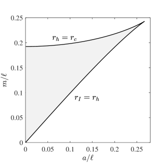
Figure 4: Parameter space for the Kerr de Sitter metric. The extremal limit $r_{I}=r_{h}$ forms the right boundary of the plot whereas the Nariai limit $r_{c}=r_{h}$ forms the upper boundary. Outside of the shaded region, one encounters naked singularities.

The mass $M$ and the angular momentum $J$ can be defined using analytic continuation from anti-de Sitter space Henneaux and Teitelboim (1985), and was studied in detail in the thermodynamical context in Dolan et al. (2013) (see also Dolan (2019)). In terms of the mass parameter $m$ and the rotation parameter $a$,

$$M={m\over\Xi^{2}},\qquad J={am\over\Xi^{2}}.$$ (12)

We take a non-minimally coupled scalar field, $\phi$, on the black hole background with field equation

$$-\nabla_{\mu}\nabla^{\mu}\phi+\xi{\cal R}\phi=0,$$ (13)

where ${\cal R}$ is the Ricci scalar and $\xi$ is the non-minimal coupling constant. Solutions are expanded in separable modes Chambers and Moss (1994b)

$$\phi=\sum_{lm_{z}}\int{d\omega\over 2\pi}{R_{\omega lm_{z}}(r)\over(r^{2}+a^{2})^{1/2}}S_{\omega lm_{z}}(\theta)e^{im_{z}\varphi}e^{-i\omega t},$$ (14)

where the $S_{\omega lm_{z}}(\theta)$’s are the angular eigenfunctions Tachizawa and Maeda (1992). We introduce a tortoise coordinate defined by

$$dr^{*}\equiv{r^{2}+a^{2}\over\Delta_{r}}dr,$$ (15)

The radial equation is then of the form

$$-\partial_{r^{*}}^{2}R_{\omega lm_{z}}+V_{\omega lm_{z}}(r)R_{\omega lm_{z}}=0$$ (16)

with the potential

$$V_{\omega lm_{z}}=-(\omega-m_{z}\Omega)^{2}+\frac{\Delta_{r}}{(r^{2}+a^{2})^{2}}\left\{\lambda+12\xi{r^{2}\over\ell^{2}}+(r^{2}+a^{2})^{1/2}\left(\frac{r\Delta_{r}}{(r^{2}+a^{2})^{3/2}}\right)^{\prime}\right\},$$ (17)

where $\lambda$ is angular eigenvalue (that depends on $l$, $m_{z}$ and $\omega$), and

$$\Omega\equiv\Xi{a\over r^{2}+a^{2}}.$$ (18)

The potential has the limit of $V\to-(\omega-m_{z}\Omega)^{2}$ on the horizons. There are ingoing or outgoing modes described here by arrows,

$${\overrightarrow{R}}\to\sqrt{\Xi\over|2\omega_{h}|}\begin{cases}e^{i\omega_{h}r^{*}}+{\overrightarrow{A}}e^{-i\omega_{h}r^{*}}&r\to r_{h}\\ {\overrightarrow{B}}e^{i\omega_{c}r^{*}}&r\to r_{c},\end{cases}$$ (19)

$${\overleftarrow{R}}\to\sqrt{\Xi\over|2\omega_{c}|}\begin{cases}{\overleftarrow{B}}e^{-i\omega_{h}r^{*}}&r\to r_{h}\\ e^{-i\omega_{c}r^{*}}+{\overleftarrow{A}}e^{i\omega_{c}r^{*}}&r\to r_{c},\end{cases}$$ (20)

where the normalisation is discussed in appendix A.

Flux conservation follows from the Wronskian relation for any two solutions $R_{1}$ and $R_{2}$,

$$\partial_{r^{*}}\left(R_{1}\partial_{r^{*}}R_{2}-R_{2}\partial_{r^{*}}R_{1}\right)=0.$$ (21)

It leads to

$$\omega_{h}(1-|\overrightarrow{A}_{\omega lm_{z}}|^{2}) =\omega_{c}|\overrightarrow{B}_{\omega lm_{z}}|^{2}$$ (22)

$$\omega_{c}(1-|\overleftarrow{A}_{\omega lm_{z}}|^{2}) =\omega_{h}|\overleftarrow{B}_{\omega lm_{z}}|^{2}$$ (23)

$$\omega_{h}\overrightarrow{B}_{\omega lm_{z}}\overrightarrow{A}^{*}_{\omega lm_{z}} =-\omega_{c}\overrightarrow{B}_{\omega lm_{z}}^{*}\overrightarrow{A}_{\omega lm_{z}}$$ (24)

$$\omega_{h}\overleftarrow{B}_{\omega lm_{z}} =\omega_{c}\overrightarrow{B}_{\omega lm_{z}}.$$ (25)

From these we also conclude that $|\overrightarrow{A}_{\omega lm_{z}}|=|\overleftarrow{A}_{\omega lm_{z}}|$, and we define the absolute value of the reflection coefficient as $A_{\omega lm_{z}}\equiv|\overrightarrow{A}_{\omega lm_{z}}|=|\overleftarrow{A}_{\omega lm_{z}}|$.

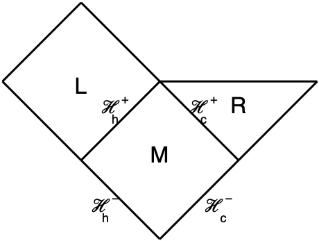
Figure 5: Part of the Penrose diagram of the black hole spacetime with the supported regions for each of the mode function. For example, $f^{M}$ is based on support on region $M$.

In true Unruh style Unruh (1976), a superscript $L$, $M$ or $R$ denotes modes with support in different parts of the extended Penrose diagram:

$$L:\quad r<r_{h},\quad U_{h}=e^{-\kappa_{h}u}$$ (26)

$$M:\quad r_{h}<r<r_{c},\quad U_{h}=-e^{-\kappa_{h}u},\quad V_{c}=-e^{-\kappa_{c}v}$$ (27)

$$R:\quad r_{c}<r,\quad V_{c}=e^{-\kappa_{c}v}$$ (28)

where $u=t-r^{\ast}$ and $v=t+r^{\ast}$ (see figure 5). The $\kappa_{h,c}$ are the surface gravities at the respective horizons which are related to temperature in the usual manner, namely $T_{h,c}=\kappa_{h,c}/2\pi$. (Note that we have taken positive surface gravities.) The explicit expression for the temperatures are,

$$T_{h,c}\equiv\beta_{h,c}^{-1}=\left|\frac{\partial_{r}\Delta_{r}|_{r=r_{h,c}}}{4\pi(r_{h,c}^{2}+a^{2})}\right|.$$ (29)

The Kruskal coordinate on the event horizon is $U_{h}$ and the Kruskal coordinate on the cosmological horizon is $V_{c}$. Let $f=R(r)e^{-i\omega t}S_{\omega lm_{z}}(\theta)e^{im_{z}\varphi}/\sqrt{r^{2}+a^{2}}$, then outgoing modes which are positive frequency in $U$ on the past event horizon are denoted by $\overrightarrow{f}^{U}$,

$$\overrightarrow{f}^{U}=\left|2\sinh\pi\omega_{h}/\kappa_{h}\right|^{-1/2}\left(e^{\pi\omega_{h}/2\kappa_{h}}\overrightarrow{f}^{M}+e^{-\pi\omega_{h}/2\kappa_{h}}\overrightarrow{f}^{L}\right),$$ (30)

where $\overrightarrow{f}^{M}$ and $\overrightarrow{f}^{L}$ are outgoing plane-wave basis of positive frequency defined in $U_{h}<0$ and $U_{h}>0$, respectively. Ingoing modes which are positive frequency in $V$ on the past cosmological horizon are denoted by $\overleftarrow{f}^{V}$,

$$\overleftarrow{f}^{V}=\left|2\sinh\pi\omega_{c}/\kappa_{c}\right|^{-1/2}\left(e^{\pi\omega_{c}/2\kappa_{c}}\overleftarrow{f}^{M}+e^{-\pi\omega_{c}/2\kappa_{c}}\overleftarrow{f}^{R}\right)$$ (31)

We can check that the $\overrightarrow{f}^{U}$ modes are positive frequency by taking a point on the horizon at $r=r_{h}$,

$$\overrightarrow{f}^{U}\to\sqrt{\Xi\over|4\omega_{h}\sinh\pi\omega_{h}/\kappa_{h}|}\left(e^{-i\omega_{h}(t-r^{*})+\pi\omega_{h}/2\kappa_{h}}\Theta(-U_{h})+e^{-i\omega_{h}(t-r^{*})-\pi\omega_{h}/2\kappa_{h}}\Theta(U_{h})\right)$$ (32)

where $\Theta$ is the Heaviside function. In terms of the Kruskal coordinate, we have

$$\overrightarrow{f}^{U}\to\sqrt{\Xi\over|4\omega_{h}\sinh\pi\omega_{h}/\kappa_{h}|}\exp\left({i\omega_{h}\over\kappa_{h}}\log(-iU_{h})\right)$$ (33)

Since the branch cut for the logarithm lies in the upper half plane, the modes are regular in the entire lower half of the complex $U_{h}$ plane. The Fourier transform in $U_{h}$ therefore vanishes when the Fourier frequency is negative.

3 Fluxes

In order to employ quantum field theory on a curved spacetime background, we assume that the backreaction effect is small, and the expectation value of the quantum energy flux $\langle\hat{T}_{rt}\rangle$ reacts back on the spacetime geometry through the Einstein field equation

$$G_{rt}=8\pi\langle\hat{T}_{rt}\rangle.$$ (34)

Following previous work Hawking (1974, 1975); Page (1976a, b); Candelas (1980), we also adopt an adiabatic approximation that assumes the spacetime metric approximates the original black hole form but with time-dependent mass and angular momentum. Note that, in the rotating case, the flux can introduce additional distortions dependent on the azimuthal angle, but we know that such distortions decay away rapidly when not driven, and therefore we do not expect to see secular growth. We remove these small distortions by averaging over the azimuthal angle.

For a non-minimally coupled scalar field, the stress energy tensor

$$T_{rt}=(1-8\pi\xi\phi^{2})^{-1}\left\{\partial_{r}\phi\partial_{t}\phi-\xi\partial_{t}\partial_{r}\phi^{2}\right\}.$$ (35)

Since the backreaction is small, and $\langle\hat{\phi}\rangle=0$, only the quadratic order terms need be retained. Following Candelas Candelas (1980), we introduce a stress tensor bilinear

$$T_{rt}(f_{1},f_{2})=\frac{1}{2}\mathrm{Re}\left[\partial_{t}f_{1}^{*}\partial_{r}f_{2}+\partial_{r}f_{1}^{*}\partial_{t}f_{2}-4\xi\partial_{r}\partial_{t}(f_{1}^{*}f_{2})\right]$$ (36)

and then the expectation value of the quantum flux operator in the vacuum state is

$$\langle T_{rt}\rangle={1\over 4\pi}\sum_{lm_{z}}\int_{-\infty}^{\infty}{d\omega\over 2\pi}\left\{T_{rt}(\overrightarrow{f}^{U},\overrightarrow{f}^{U})+T_{rt}(\overleftarrow{f}^{V},\overleftarrow{f}^{V})\right\}.$$ (37)

In the rotating case, this will depend on the azimuthal angle $\theta$. We include the additional average over $\theta$ in the definition of $\langle\langle\rangle\rangle$ to remove this dependence.

Consider the flux as $r\to r_{c}$, inserting the explicit expressions for the modes from Eq. (19),

$$\langle\langle T_{rt}\rangle\rangle=-{\Xi\over 4\pi\Delta_{r}}\sum_{lm_{z}}\int_{-\infty}^{\infty}{d\omega\over 2\pi}{\omega\over 2}\left\{{\omega_{c}\over\omega_{h}}|\overrightarrow{B}_{\omega lm_{z}}|^{2}{e^{\beta_{h}\omega_{h}}\over e^{\beta_{h}\omega_{h}}-1}-(1-|A_{\omega lm_{z}}|^{2}){e^{\beta_{c}\omega_{c}}\over e^{\beta_{c}\omega_{c}}-1}\right\}.$$ (38)

After using the flux rules Eqs. (25) and the symmetry $A_{-\omega l-m}=A_{\omega lm}$,

$$\langle\langle T_{rt}\rangle\rangle=-{\Xi\over 4\pi\Delta_{r}}\sum_{lm_{z}}\int_{0}^{\infty}{d\omega\over 2\pi}\omega\left(1-|A_{\omega lm_{z}}|^{2}\right)\frac{1}{2}\left\{{\rm coth}{\beta_{h}\omega_{h}\over 2}-{\rm coth}{\beta_{c}\omega_{c}\over 2}\right\}.$$ (39)

Due to the constancy of the Wronskian (21), the expression under the integral is independent of the radius we choose to evaluate $T_{rt}$. The factor of $\Delta_{r}^{-1}$ comes from the derivative $dr^{\ast}/dr$ and the divergence of $1/\Delta_{r}$ at the cosmological horizon is relevant to the blue shift effect although the mass-loss and spin-loss rates are regular as is shown later. Consequently, the only $r$ dependence appearing in (39) is contained in the prefactor $\Delta_{r}^{-1}$. For the rotation, consider $T_{r\varphi}$,

$$\langle\langle T_{r\varphi}\rangle\rangle={\Xi\over 4\pi\Delta_{r}}\sum_{lm_{z}}\int_{0}^{\infty}{d\omega\over 2\pi}m_{z}\left(1-|A_{\omega lm_{z}}|^{2}\right)\frac{1}{2}\left\{{\rm coth}{\beta_{h}\omega_{h}\over 2}-{\rm coth}{\beta_{c}\omega_{c}\over 2}\right\}.$$ (40)

The rate of mass loss can be found in an adiabatic approximation by replacing $m$ and $a$ by a functions $m(t)$ and $a(t)$, then the relevant Einstein tensor components averaged over angles becomes

$$\langle\langle G_{rt}\rangle\rangle ={2\over\Delta_{r}\Xi}\left(\Xi\dot{m}-3{a\over\ell^{2}}m\dot{a}\right),$$ (41)

$$\langle\langle G_{r\varphi}\rangle\rangle ={2\over\Delta_{r}\Xi^{2}}\left(\left(3{a^{2}\over\ell^{2}}-1\right)m\dot{a}-a\Xi\dot{m}\right),$$ (42)

Using $M=m/\Xi^{2}$ and $J=am/\Xi^{2}$ for the slowly evolving background spacetime,

$$\langle\langle G_{rt}\rangle\rangle+{a\over\ell^{2}}\langle\langle G_{r\varphi}\rangle\rangle =\Xi{2\over\Delta_{r}}{dM\over dt},$$ (43)

$$\langle\langle G_{r\varphi}\rangle\rangle =-\Xi{2\over\Delta_{r}}{dJ\over dt}.$$ (44)

Hence, relating these to the fluxes by Eq. (34),

$${dM\over dt}=-\sum_{lm_{z}}\int_{0}^{\infty}{d\omega\over 2\pi}\left(\omega-{am_{z}\over\ell^{2}}\right)\left(1-|A_{\omega lm_{z}}|^{2}\right)\frac{1}{2}\left\{{\rm coth}{\beta_{h}\omega_{h}\over 2}-{\rm coth}{\beta_{c}\omega_{c}\over 2}\right\}.$$ (45)

and for the angular momentum,

$${dJ\over dt}=-\sum_{lm_{z}}\int_{0}^{\infty}{d\omega\over 2\pi}m_{z}\left(1-|A_{\omega lm_{z}}|^{2}\right)\frac{1}{2}\left\{{\rm coth}{\beta_{h}\omega_{h}\over 2}-{\rm coth}{\beta_{c}\omega_{c}\over 2}\right\}.$$ (46)

Note that due to the definition of $\Omega$ in (18), the factor $\omega-am_{z}/\ell^{2}$ in (45) is equivalent to $\omega-m_{z}\Omega(\ell)$, i.e. the frequency in the rotating frame at $r=\ell$. Indeed, in black hole thermodynamics in de Sitter space, the angular velocities appearing in the first laws for the two horizons are $\Omega_{h,c}=\Omega(r_{h,c})-\Omega(\ell)$ Dolan et al. (2013). Thus, one would expect the relevant frequency for the change in thermodynamic mass $M$ to be the one that appears in (45).

We have been assuming that the energy fluxes affect the mass and spin of the black hole, but there has been some discussion elsewhere about whether quantum processes could cause the decay of the vacuum energy in de Sitter space Mottola (1985); Abramo, Brandenberger, and Mukhanov (1997); Anderson and Mottola (2014); Markkanen (2016). In order to examine this possibility, we let $\ell\to\ell(t)$ and examine the angle averaged $G_{rt}$ Einstein tensor component,

$$\langle G_{rt}\rangle=2{\dot{m}\over\Delta_{r}}-{6ma\over\ell^{2}\Xi}{\dot{a}\over\Delta_{r}}+{6ma^{2}\over\ell^{3}\Xi}{\dot{\ell}\over\Delta_{r}}-{(a^{2}+r^{2})r\over\ell^{3}}{\dot{\ell}\over\Delta_{r}}.$$ (47)

The first three terms match the radial dependence in the fluxes, but the final term does not. We conclude that decay of vacuum energy is not consistent with the backreaction calculation in the vacuum state that we are using.

4 Evaporation process of a spinning BH with a cosmological constant

In this section, we describe how we compute numerically the time-development of a spinning black hole with a cosmological constant.

4.1 Methodology

Following the earlier work of Page Page (1976b), we assume the angular momentum $J(t)$ is monotonically decreasing, and choose the spin parameter $a$ as the independent variable characterizing the evolution of a rotating black hole, i.e.

$$M(t)\ \text{and}\ J(t)\to M(a)\ \text{and}\ t(a).$$ (48)

A large dynamical range can be investigated using logarithmic variables,

$$y \equiv-\ln{(a/a_{0})},$$ (49)

$$z \equiv-\ln{(M/M_{0})},$$ (50)

where $a_{0}$ and $M_{0}$ are the initial spin parameter and mass. The function $z(y)$ evolves as

$$\frac{dz}{dy}=\frac{f}{g-f}.$$ (51)

where

$$f =-M^{3}\frac{d\ln{(M/M_{0})}}{dt},$$ (52)

$$g =-M^{3}\frac{d\ln{(J/J_{0})}}{dt},$$ (53)

The mass and angular momentum loss rates are evaluated numerically using (45) and (46).

Finally, the scale-invariant time parameter, $\tau$, is defined as

$$\tau\equiv\frac{t}{M_{0}^{3}},$$ (54)

and the evolution of $\tau(y)$ is governed by

$$\frac{d\tau}{dy}=\frac{e^{-3z}}{g-f}.$$ (55)

We solve the two ordinary differential equations (ODEs), (51) and (55), with the fourth-order Runge-Kutta method while the values of $f$ and $g$ are obtained as explained below.

4.2 Teukolsky equation and the Heun function

For the analysis of the linear perturbations of gravitational, electromagnetic, neutrino, and scalar fields, it is important to estimate the greybody factor. Let us consider a mode function ${}_{s}\psi_{lm_{z}}(t,r,\theta,\varphi)$, where $s$ is the spin of the field, which can be expanded as

$${}_{s}\psi_{lm_{z}}(t,r,\theta,\varphi)=\int\frac{d\omega}{2\pi}e^{-i\omega t}e^{im_{z}\varphi}{}_{s}R^{{(\rm T)}}_{\omega lm_{z}}(r){}_{s}S_{\omega lm_{z}}(\theta).$$ (56)

Note that the radial function $R_{\omega lm_{z}}$ introduced in (14) is related to ${}_{s}R_{\omega lm_{z}}^{{(\rm T)}}$ as $R_{\omega lm_{z}}=(r^{2}+a^{2})^{1/2}{}_{0}R^{{(\rm T)}}_{\omega lm_{z}}$. It was shown that the functions ${}_{s}R^{{(\rm T)}}_{\omega lm_{z}}(r)$ and ${}_{s}S_{\omega lm_{z}}(\theta)$ are solutions of the following Teukolsky equations by Suzuki, Takasugi, and Umetsu in Ref. Suzuki, Takasugi, and Umetsu (1998):

$$\left[\frac{d}{dq}\Delta_{q}\frac{d}{dq}-\frac{1}{\Delta_{q}}\left(\tilde{V}+\frac{s}{2}\Delta_{q}^{\prime}\right)^{2}+2s\tilde{V}^{\prime}-{}_{s}X_{\omega lm_{z}}\right]{}_{s}S_{\omega lm_{z}} =0,$$ (57)

$$\left[\Delta_{r}^{-s}\frac{d}{dr}\Delta_{r}^{s+1}\frac{d}{dr}+\frac{1}{\Delta_{r}}\left(\tilde{W}^{2}-is\tilde{W}\Delta_{r}^{\prime}\right)+2is\tilde{W}^{\prime}-{}_{s}Y_{\omega lm_{z}}\right]{}_{s}R^{{(\rm T)}}_{\omega lm_{z}} =0,$$ (58)

where

$$\tilde{V}(q) \equiv a\omega(1-q^{2})-\Xi m,$$ (59)

$$\tilde{W}(r) \equiv\omega(r^{2}+a^{2})-\Xi am,$$ (60)

$${}_{s}X_{\omega lm_{z}}(q) \equiv 2(2s^{2}+1)\alpha^{2}q^{2}-{}_{s}\lambda_{\omega lm_{z}},$$ (61)

$${}_{s}Y_{\omega lm_{z}}(r) \equiv 2\ell^{-2}(s+1)(2s+1)r^{2}+{}_{s}\lambda_{\omega lm_{z}}-s(1-\alpha^{2}),$$ (62)

$$\Delta_{q} \equiv(1-q^{2})(1+\alpha^{2}q^{2}),$$ (63)

$$q \equiv\cos\theta,$$ (64)

$$\alpha \equiv a/\ell,$$ (65)

and ${}_{s}\lambda_{\omega lm_{z}}$ is the angular eigenvalue. The prime in $\Delta_{q}^{\prime}(q)$ and $\Delta_{r}^{\prime}(r)$ denotes the derivative with respect to $q$ and $r$, respectively. Note that the Teukolsky equations with $s=0$ describe perturbations of a massless conformally coupled scalar field. In the following, for scalar perturbations, we will deal with the conformally coupled scalar field ($\xi=1/6$) only. The angular eigenvalue ${}_{s}\lambda_{\omega lm_{z}}$ is determined by a boundary condition requiring the regularity for ${}_{s}S_{\omega lm_{z}}$ at $q=\pm 1$. As shown in Suzuki, Takasugi, and Umetsu (1998), this boundary value problem can be solved by the Heun function. Let us implement the following transformations in (57):

$$z \equiv\frac{(1-i/\alpha)(1+q)}{2(q-i/\alpha)},$$ (66)

$${}_{s}\tilde{S}_{\omega lm_{z}}(z) \equiv z^{-A_{1}}(z-1)^{-A_{2}}(z-z_{a})^{-A_{3}}(z-z_{a\infty})^{-1}{}_{s}S_{\omega lm_{z}}(q),$$ (67)

where

$$z_{a} \equiv-\frac{(1-i/\alpha)^{2}}{4i/\alpha},$$ (68)

$$z_{a\infty} \equiv\frac{1-i/\alpha}{2},$$ (69)

and

$$A_{1}\equiv\frac{m-s}{2},\ \ \ A_{2}\equiv-\frac{m+s}{2},\ \ \ A_{3}\equiv\frac{i}{2}\left(\frac{c}{\alpha}-m\alpha-is\right)$$ (70)

with $c\equiv a\omega$. In the following, we often omit the subscripts $(s,\omega,l,m_{z})$. The function $\tilde{S}(z)$ satisfies the following ODE

$$\tilde{S}^{\prime\prime}+\left(\frac{2A_{1}+1}{z}+\frac{2A_{2}+1}{z-1}+\frac{2A_{3}+1}{z-z_{a}}\right)\tilde{S}^{\prime}+\frac{F_{a}^{(+)}F_{a}^{(-)}z+G_{a}}{z(z-1)(z-z_{a})}\tilde{S}=0,$$ (71)

where a prime denotes the derivative with respect to $z$ and

$$F_{a}^{(+)} \equiv 1,\ F_{a}^{(-)}\equiv 1-s-im\alpha+i\frac{c}{\alpha},$$ (72)

$$G_{a} \equiv-\left[\frac{i\lambda}{4\alpha}+\frac{1}{2}+A_{1}+\left(m+\frac{1}{2}\right)(A_{3}-A_{3}^{\ast})\right].$$ (73)

Eq. (71) is nothing but Heun’s differential equation. One can obtain the analytic solutions at $z=0$ ($q=-1$) and $z=1$ ($q=+1$) with the general Heun function denoted by “HeunG”. Indeed, the radial part (58) can be also transformed into Heun’s differential equation. Let us implement the M$\ddot{\rm o}$bius transformation

$$z=\frac{(r_{c}-r_{h}^{\prime})(r-r_{h})}{(r_{c}-r_{h})(r-r_{h}^{\prime})},$$ (74)

and define a new variable

$$\tilde{R}^{{(\rm T)}}(z)\equiv z^{-B_{1}}(z-1)^{-B_{2}}(z-z_{r})^{-B_{3}}(z-z_{r\infty})^{-2s-1}R^{{(\rm T)}}(r),$$ (75)

with

$$B_{1}\equiv\frac{i\tilde{W}(r_{h})}{\Delta_{r}^{\prime}(r_{h})},\ \ \ B_{2}\equiv\frac{i\tilde{W}(r_{c})}{\Delta_{r}^{\prime}(r_{c})},\ \ \ B_{3}\equiv\frac{i\tilde{W}(r_{c}^{\prime})}{\Delta_{r}^{\prime}(r_{c}^{\prime})},$$ (76)

$$z_{r}\equiv\frac{(r_{c}-r_{h}^{\prime})(r_{c}^{\prime}-r_{h})}{(r_{c}-r_{h})(r_{c}^{\prime}-r_{h}^{\prime})},\ \ \ z_{r\infty}\equiv\frac{r_{c}-r_{h}^{\prime}}{r_{c}-r_{h}}.$$ (77)

Here $r_{c}^{\prime}$, $r_{h}^{\prime}$, $r_{h}$, and $r_{c}$ are four roots of $\Delta_{r}(r)=0$ and they satisfy $r_{c}^{\prime}<r_{h}^{\prime}<r_{h}<r_{c}$. Note that the outer horizon at $r=r_{h}$ and cosmological horizon at $r=r_{c}$ correspond to $z=0$ and $z=1$, respectively. Then we obtain Heun’s differential equation

$$\begin{split}\tilde{R}^{{(\rm T)}}{}^{\prime\prime}+\left(\frac{2B_{1}+s+1}{z}+\frac{2B_{2}+s+1}{z-1}+\frac{2B_{3}+s+1}{z-z_{r}}\right)\tilde{R}^{{(\rm T)}}{}^{\prime}&\\ +\frac{F_{r}^{(+)}F_{r}^{(-)}z+G_{r}}{z(z-1)(z-z_{r})}\tilde{R}^{{(\rm T)}}=0&,\end{split}$$ (78)

where

$$F_{r}^{(+)} \equiv 2s+1,\ F_{r}^{(-)}\equiv s+1-\frac{2i\tilde{W}(r_{h}^{\prime})}{\Delta_{r}^{\prime}(r_{h}^{\prime})},$$ (79)

$$\begin{split}G_{r}&\equiv\frac{(1+s)(1+2s)r_{c}^{\prime}}{r_{h}^{\prime}-r_{c}^{\prime}}+\frac{\ell^{2}[\lambda-2s(1-\alpha^{2})]+(1+s)(1+2s)r_{h}(r_{c}+r_{h})}{(r_{h}^{\prime}-r_{c}^{\prime})(r_{h}-r_{c})}\\ &-\frac{2i\ell^{2}\Xi(1+2s)(r_{h}r_{h}^{\prime}\omega+a^{2}\omega/\Xi-am)}{(r_{h}^{\prime}-r_{c}^{\prime})(r_{h}^{\prime}-r_{h})(r_{h}-r_{c})}.\end{split}$$ (80)

Heun’s differential equation in a general form is

$$y^{\prime\prime}(z)+\left(\frac{\gamma}{z}+\frac{\delta}{z-1}+\frac{\epsilon}{z-k}\right)y^{\prime}(z)+\frac{\zeta\beta z-w}{z(z-1)(z-k)}y(z)=0,$$ (81)

with $\gamma+\delta+\epsilon=\zeta+\beta+1$. Heun’s equation has four regular singular points at $z=0$, $z=1$, $z=k$, and $z=\infty$. One can construct local solutions for each singular point, and those solutions are convergent inside a circle. The radius of the convergence is determined by the distance from the neighbour singular point. In our analysis, we need two local solutions at $z=0$ and $z=1$. The general solution near $z=0$ is given by the linear combination of Hatsuda (2020)

$$y_{01}(z) =\text{HeunG}(k,w;\zeta,\beta,\gamma,\delta;z),$$ (82)

$$y_{02}(z) =z^{1-\gamma}\text{HeunG}(k,(k\delta+\epsilon)(1-\gamma)+w;\zeta+1-\gamma,\beta+1-\gamma,2-\gamma,\delta;z),$$ (83)

and the general solution near $z=1$ is represented by the linear combination of

$$y_{11}(z) =\text{HeunG}(1-k,\zeta\beta-w;\zeta,\beta,\delta,\gamma;1-z),$$ (84)

$$\begin{split}y_{12}(z)&=(1-z)^{1-\delta}\\ &\times\text{HeunG}(1-k,p;\zeta+1-\delta,\beta+1-\delta,2-\delta,\gamma;1-z),\end{split}$$ (85)

where $p\equiv((1-k)\gamma+\epsilon)(1-\delta)+\zeta\beta-w$. Let the function $y_{Aij}(z)$ be defined as $y_{ij}(z)$ with the values

$$\begin{split}&\gamma\to 2A_{1}+1,\ \delta\to 2A_{2}+1,\ \epsilon\to 2A_{3}+1,\\ &\zeta\to F_{a}^{(+)},\ \beta\to F_{a}^{(-)},\ w\to G_{a},\end{split}$$ (86)

and $y_{Rij}(z)$ is defined by $y_{ij}(z)$ with

$$\begin{split}&\gamma\to 2B_{1}+1,\ \delta\to 2B_{2}+1,\ \epsilon\to 2B_{3}+1,\\ &\zeta\to F_{r}^{(+)},\ \beta\to F_{r}^{(-)},\ w\to G_{r}.\end{split}$$ (87)

Then the two solutions of the angular equation near $z=0$ ($q=-1$) is given by

$$S_{01}(q) \equiv z^{A_{1}}(z-1)^{A_{2}}(z-z_{a})^{A_{3}}(z-z_{\infty})y_{A01}(z)\propto(1+u)^{(m_{z}-s)/2},$$ (88)

$$S_{02}(q) \equiv z^{A_{1}}(z-1)^{A_{2}}(z-z_{a})^{A_{3}}(z-z_{\infty})y_{A02}(z)\propto(1+u)^{-(m_{z}-s)/2},$$ (89)

and near $z=1$ ($q=+1$), we have

$$S_{11}(q) \equiv z^{A_{1}}(z-1)^{A_{2}}(z-z_{a})^{A_{3}}(z-z_{\infty})y_{A11}(z)\propto(1-u)^{-(m_{z}+s)/2},$$ (90)

$$S_{12}(q) \equiv z^{A_{1}}(z-1)^{A_{2}}(z-z_{a})^{A_{3}}(z-z_{\infty})y_{A12}(z)\propto(1-u)^{(m_{z}+s)/2}.$$ (91)

In order for the solution to be regular at $q=\pm 1$, one has to properly choose the boundary solutions at $q=\pm 1$. As an example, let us consider the case of $(s,m_{z})=(1,0)$. In this case, the solution at $q=-1$ and $q=+1$ should be $\sim S_{02}(q)$ and $\sim S_{12}(q)$, respectively, in order for the solution to be regular. Such a situation is realized when those two solutions are linearly dependent, which is equivalent to

$$W[y_{A02},y_{A12}]=0,$$ (92)

and this condition determines the angular eigenvalue $\lambda_{slm}$. We search the exact value of $\lambda_{slm_{z}}$ by using the function FindRoot in Mathematica.

4.3 Greybody factor and superradiance

We calculate the greybody factor by using the analytic solutions of the Teukolsky equation, represented by the general Heun function. Using the analytic solutions of Heun’s equation at $z=0$ and $z=1$, the two independent radial solutions near the outer horizon $r=r_{h}$ ($z=0$)

$$R_{+}^{(h)} \equiv z^{B_{1}}(z-1)^{B_{2}}(z-z_{r})^{B_{3}}(z-z_{\infty})^{2s+1}y_{R01}(z),$$ (93)

$$R_{-}^{(h)} \equiv z^{B_{1}}(z-1)^{B_{2}}(z-z_{r})^{B_{3}}(z-z_{\infty})^{2s+1}y_{R02}(z),$$ (94)

and near the cosmological horizon $r=r_{c}$ ($z=1$), we have

$$R_{+}^{(c)} \equiv z^{B_{1}}(z-1)^{B_{2}}(z-z_{r})^{B_{3}}(z-z_{\infty})^{2s+1}y_{R11}(z),$$ (95)

$$R_{-}^{(c)} \equiv z^{B_{1}}(z-1)^{B_{2}}(z-z_{r})^{B_{3}}(z-z_{\infty})^{2s+1}y_{R12}(z).$$ (96)

In the near-horizon limit, those solutions reduce to purely ingoing or outgoing modes

$$R_{\pm}^{(h)}\simeq C_{\pm}^{(h)}(r-r_{h})^{-\frac{s}{2}\pm\theta_{h}},\ \theta_{h}\equiv i\frac{\omega_{h}}{2\kappa_{h}}+\frac{s}{2},$$ (97)

$$R_{\pm}^{(c)}\simeq C_{\pm}^{(c)}(r-r_{c})^{-\frac{s}{2}\pm\theta_{c}},\ \theta_{c}\equiv i\frac{\omega_{c}}{2\kappa_{c}}+\frac{s}{2},$$ (98)

where $\kappa_{h/c}\equiv 2\pi/\beta_{h/c}$ and

$$C_{\pm}^{(h)} \equiv(-1)^{B_{2}}\left(\frac{r_{c}-r_{h}^{\prime}}{(r_{c}-r_{h})(r_{h}-r_{h}^{\prime})}\right)^{-\frac{s}{2}\pm\theta_{h}}\left(\frac{(r_{c}-r_{h}^{\prime})(r_{h}-r_{c}^{\prime})}{(r_{c}-r_{h})(r_{c}^{\prime}-r_{h}^{\prime})}\right)^{B_{3}}\left(\frac{r_{h}^{\prime}-r_{c}}{r_{c}-r_{h}}\right)^{2s+1},$$ (99)

$$C_{\pm}^{(c)} \equiv\left(\frac{r_{h}-r_{h}^{\prime}}{(r_{c}-r_{h})(r_{c}-r_{h}^{\prime})}\right)^{-\frac{s}{2}\pm\theta_{c}}\left(\frac{(r_{h}-r_{h}^{\prime})(r_{c}-r_{c}^{\prime})}{(r_{c}-r_{h})(r_{c}^{\prime}-r_{h}^{\prime})}\right)^{B_{3}}\left(\frac{r_{h}^{\prime}-r_{h}}{r_{c}-r_{h}}\right)^{2s+1}.$$ (100)

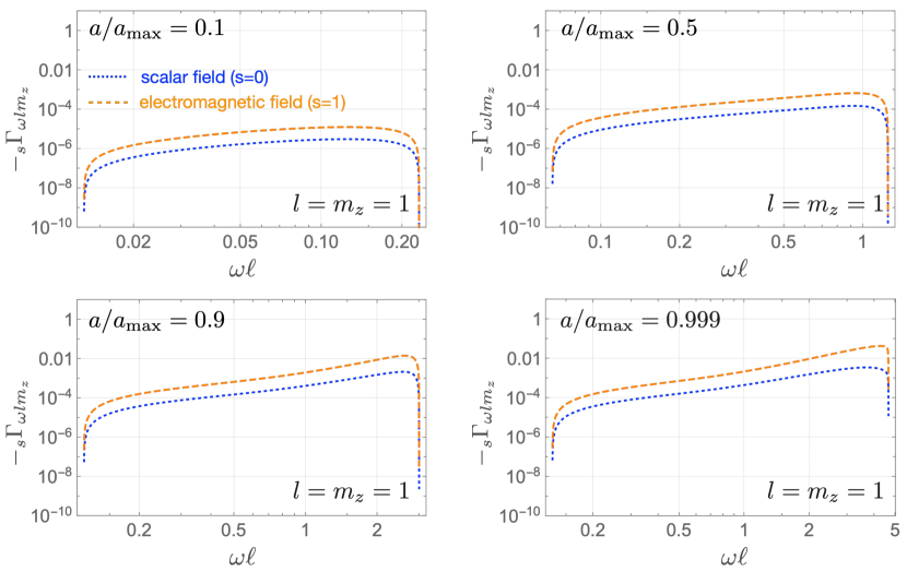
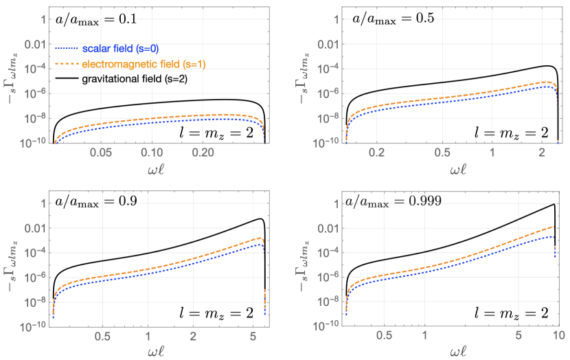
Figure 6: Plot of $-{}_{s}\Gamma_{\omega lm_{z}}$ in the frequency range showing superradiance. We set $m/\ell=0.1$ and $a_{\rm max}$ is the spin parameter at the extremal situation with $m/\ell=0.1$.

Let us consider the solution for which the mode function is purely outgoing at $r=r_{c}$

$${}_{s}R^{{(\rm T)}}_{\omega lm_{z}}=\begin{cases}{}_{s}B_{\omega lm_{z}}(r-r_{c})^{i\frac{\omega_{c}}{2\kappa_{c}}}&r\to r_{c},\\ \displaystyle(r-r_{h})^{i\frac{\omega_{h}}{2\kappa_{h}}}+{}_{s}A_{\omega lm_{z}}(r-r_{h})^{-i\frac{\omega_{h}}{2\kappa_{h}}-s}&r\to r_{+},\end{cases}$$ (101)

and the coefficients are given by

$$\frac{1}{{}_{s}B_{\omega lm_{z}}}=\frac{C_{+}^{(h)}}{C_{+}^{(c)}}\frac{W[y_{11},y_{02}]}{W[y_{01},y_{02}]},$$ (102)

$$\frac{{}_{s}A_{\omega lm_{z}}}{{}_{s}B_{\omega lm_{z}}}=\frac{C_{-}^{(h)}}{C_{+}^{(c)}}\frac{W[y_{11},y_{01}]}{W[y_{02},y_{01}]}.$$ (103)

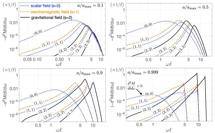
Figure 7: The spectra of energy fluxes carrying out the mass of KdS black hole. The spectra are computed with respect to various combinations of $(l,m_{z})$. The mass parameter is fixed with $m/\ell=0.1$. Note that the mass-change rate of the scalar component of $(0,0)$ mode for $a/a_{{\rm max}}=0.999$ is positive although it is negligible.

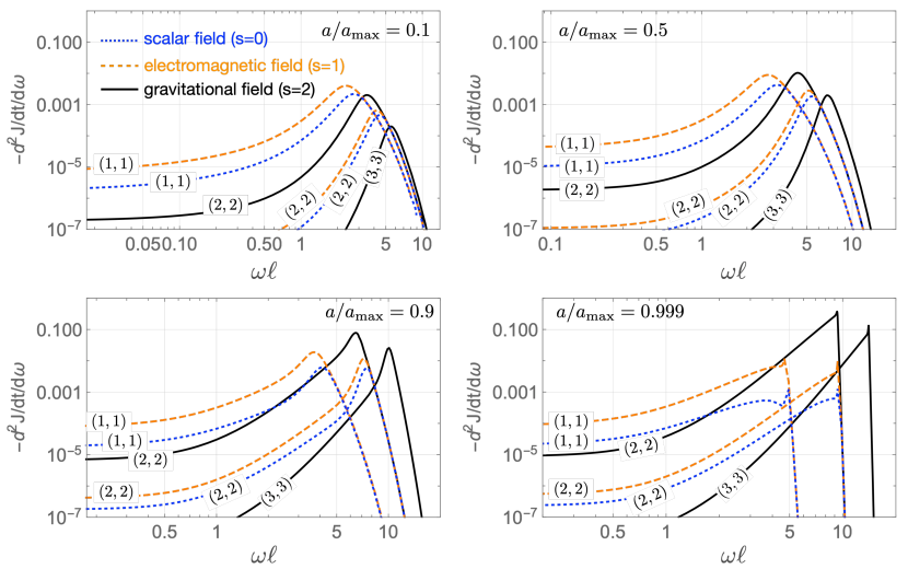
Figure 8: The spectra of energy fluxes carrying out the angular momentum of KdS black hole. The parameter set is same as figure 7.

Using the Wronskian for the solutions of Teukolsky equation

$${}_{s}{\cal W}[u_{1},u_{2}]\equiv-i\Delta_{r}^{s+1}(r)\left(u_{1}\frac{du_{2}}{dr}-u_{2}\frac{du_{1}}{dr}\right),$$ (104)

whose real part gives the energy flux, one can obtain the following relation Novaes et al. (2019)

$$({}_{s}A_{\omega lm_{z}})({}_{-s}A_{\omega lm_{z}}^{\ast})+({}_{s}\tau_{\omega lm_{z}}^{-1})({}_{s}B_{\omega lm_{z}})({}_{-s}B_{\omega lm_{z}}^{\ast})=1,$$ (105)

where the function ${}_{s}\tau_{\omega lm_{z}}$ is defined as

$${}_{s}\tau_{\omega lm_{z}}\equiv\frac{\theta_{h}\Delta_{r}^{\prime}(r_{h})}{\theta_{c}\Delta_{r}^{\prime}(r_{c})}.$$ (106)

The Wronskian (104) is constant in $r$ when $u_{1}$ and $u_{2}$ are the solutions of the Teukolsky equation. Then the greybody factor, ${}_{s}\Gamma_{\omega lm_{z}}$, (transmissivity) is given by

$${}_{s}\Gamma_{\omega lm_{z}}=1-({}_{s}A_{\omega lm_{z}})({}_{-s}A_{\omega lm_{z}}^{\ast})=({}_{s}\tau_{\omega lm_{z}}^{-1})({}_{s}B_{\omega lm_{z}})({}_{-s}B_{\omega lm_{z}}^{\ast})\,.$$ (107)

Now we can compute the greybody factor by using (102), (103), and (107). Our high-accuracy computation shows the superradiance, which is quantified by the greybody factor. The greybody factors for (conformal-coupling) scalar, electromagnetic, and gravitational perturbations in the superradiance-frequency band, $m_{z}\Omega_{c}\leq\omega\leq m_{z}\Omega_{h}$, are shown in figure 6.

4.4 Hawking spectrum

We compute the spectrum of the energy fluxes for conformal scalar field, photon and graviton emission. It was shown that the energy fluxes of the photon and graviton in the Kerr geometry are simply related to the Wronskians of the normalised modes to the appropriate Teukolsky equation Teukolsky and Press (1974); Chandrasekhar (1985). The analogous result for Kerr-de Sitter (KdS) can be found in Refs. Suzuki, Takasugi, and Umetsu (2000); Novaes et al. (2019), where it was shown that the constant Wronskian can be mapped into the conservation law of energy flux, from which one can implicitly derive the form of energy flux in KdS spacetime for a massless spin-$s$ field. They also confirmed that the greybody factor of KdS spacetime obtained in the Wronskian analysis is consistent with that of Kerr spacetime in the limit of $\ell\to\infty$. The fluxes are therefore determined by the greybody factors found above.

The evolution of the mass and angular momentum are given by,

$$\frac{d^{2}M}{dtd\omega}=-\sum_{slm_{z}}\frac{1}{2\pi}\left(\omega-am_{z}/\ell^{2}\right){}_{s}\Gamma_{\omega lm_{z}}\frac{1}{2}\left\{\coth{\left(\frac{\beta_{h}\omega_{h}}{2}\right)}-\coth{\left(\frac{\beta_{c}\omega_{c}}{2}\right)}\right\},$$ (108)

and

$$\frac{d^{2}J}{dtd\omega}=-\sum_{slm_{z}}\frac{m_{z}}{2\pi}{}_{s}\Gamma_{\omega lm_{z}}\frac{1}{2}\left\{\coth{\left(\frac{\beta_{h}\omega_{h}}{2}\right)}-\coth{\left(\frac{\beta_{c}\omega_{c}}{2}\right)}\right\},$$ (109)

for gravitational, electromagnetic, and conformal-coupling scalar field (figure 7 and 8). The scalar field significantly contributes to the mass-loss rate of the black hole at lower spin parameters. On the other hand, the energy flux of gravitons is dominant at higher-spin parameters due to the superradiance. In fact, the rate of change of mass associated with the scalar field of $(l,m_{z})=(0,0)$, which does not superradiate, is positive for the near-extremal case where the black hole temperature is smaller than that of the cosmological horizon. However, the contribution of this mode is negligible compared to the other components, and the total rate of change of mass is still negative. The mass-loss and spin-loss rates, $dM/dt$ and $dJ/dt$, are computed in the spin-mass parameter space in figure 9 for graviton-emission as an example. (The computation of $M(t)$ and $J(t)$ including the contribution of multiple species and modes are performed and the results are shown in FIG. 13 and 14.). For the Nariai case, $r_{h}=r_{c}$, the horizon frequencies, $\Omega_{h}$ and $\Omega_{c}$, and horizon temperatures, $1/\beta_{h}$ and $1/\beta_{c}$, are equivalent (figure 10). Nevertheless, the energy flux from the black hole does not balance exactly with that from the cosmological horizon. The energy (angular momentum) flux $dM/dt$ ($dJ/dt$), measured in the Boyer-Lindquist time $t$, is suppressed by $(r_{c}-r_{h})$ near the Nariai limit (see appendix B) whereas the blueshift factor, $dt/d\tau\propto 1/\sqrt{\Delta_{r}}$, is proportional to $(r_{c}-r_{h})^{-1}$, where $\tau$ is the proper time of an observer in the region between the two horizons. Therefore, the energy and angular momentum fluxes measured by the observer, $dM/d\tau$ and $dJ/d\tau$, are in general finite and non-zero, even in the Nariai limit.

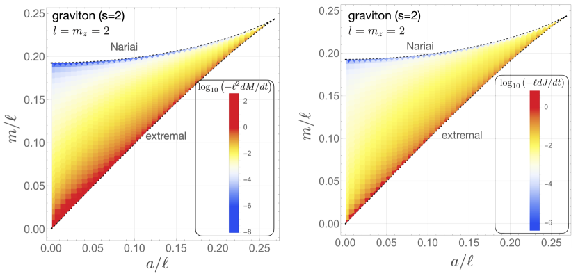
Figure 9: The mass-loss and spin-loss rates in the spin-mass parameter space. Here we computed the contribution of graviton-emission with $l=m_{z}=2$ only. The mass-loss and spin-loss rates at the Nariai limit vanish because of the zero net flux of Hawking radiation emitted from the black hole and cosmological horizons.

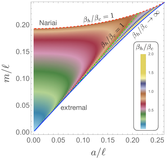
Figure 10: The ratio of the cosmological temperature to black hole temperature in the spin-mass parameter space.

We evaluate the vector field

$$\vec{v}_{H}(a,m)\equiv\left(\frac{da}{dt},\frac{dm}{dt}\right),$$ (110)

and it is shown in figure 11. One might wonder whether there are any trajectories which end at the Nariai limit, since this would be a counter example to the expectation that black holes should eventually completely evaporate away. However, our calculations indicate that the flow in (110) runs parallel to the Nariai line, which means that the Nariai solution cannot be an attractor solution, at least when graviton-emission dominates the Hawking radiation.

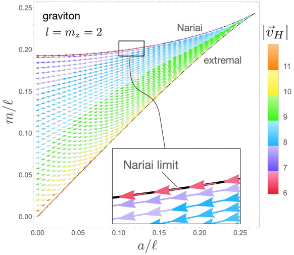
Figure 11: Stream map showing the time evolution of the KdS spacetime by taking into account graviton emission only ($l=m_{z}=2$).

As seen from figure 9 and 11, energy and angular momentum fluxes are higher near the extremal and lower-mass region. This is relevant to the intensity of superradiance which can be quantified by the greybody factor. We evaluated the maximum value of the greybody factor for $a/a_{\rm max}=0.99999$ as a function of $m$ (see figure 12). We find out that the cosmological constant quenches the effect of superradiance. One can see that the value of amplification factor in the limit of $m/\ell\to 0$ goes to the maximum amplification factor for Kerr spacetime, which was evaluated in Teukolsky and Press (1974); Rosa (2017).

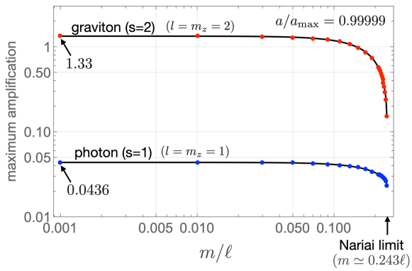
Figure 12: The maximum values of the greybody factors of graviton ($l=m_{z}=2$) and photon ($l=m_{z}=1$) for various values of $m$. We take the near-extremal limit with $a/a_{\rm max}=0.99999$.

4.5 Time evolution

We compute the time evolution of a spinning black hole in the near-extremal limit by taking into account gravitons with $(l,m_{z})=(2,2)$ and $(3,3)$, photons with $(1,1)$ and $(2,2)$, and scalar perturbations with $(0,0)$ and $(1,1)$. We numerically integrate the differential equations (51) and (55) by the 4th-order Runge-Kutta algorithm at 40 steps in $y$. The result is presented in figure 13 where we show the time-development of $J$ and $M$ computed individually for each component. One can see that the spin and mass-loss rates are dominantly governed by graviton-emission. This is consistent with the spectra shown in figure 7 and 8.

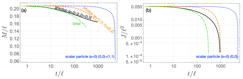
Figure 13: The time-development of (a) mass and (b) angular momentum with a near-extremal initial condition of $(a,m)=(0.255\ell,0.2355\ell)$.

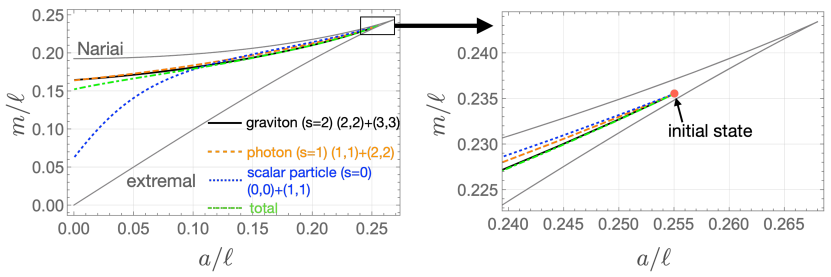
Figure 14: Trajectories of the KdS black hole on the $a$-$m$ plane. We set the same initial condition as in figure 13.

The trajectories of the KdS black hole are shown in the spin-mass parameter space (figure 14). In the slow-rotation case, the $(0,0)$ component of the scalar emission (monopole radiation) carries out the large amount of mass energy since a slowly spinning black hole is almost spherical.

The thermodynamics of the black hole and cosmological horizons have been investigated by Dolan et al. Dolan et al. (2013). It is interesting to consider the evolution of the entropy of the KdS black hole system, as typically the black hole horizon will shrink, however, the cosmological horizon also grows as the black hole loses mass and spins down. In figure 15, we show the time-development of the Bekenstein-Hawking entropy of the KdS black hole and cosmological horizon, which have the forms of

$$S_{h}\equiv\frac{\pi(r_{h}^{2}+a^{2})}{\Xi},\qquad S_{c}\equiv\frac{\pi(r_{c}^{2}+a^{2})}{\Xi},$$ (111)

respectively, and the total entropy is $S_{\rm total}\equiv S_{h}+S_{c}$. As conjectured by the generalized second law of thermodynamics, we confirm that the total entropy monotonically increases, which means that the generalized second law is satisfied even for the evaporation process of a KdS black hole.

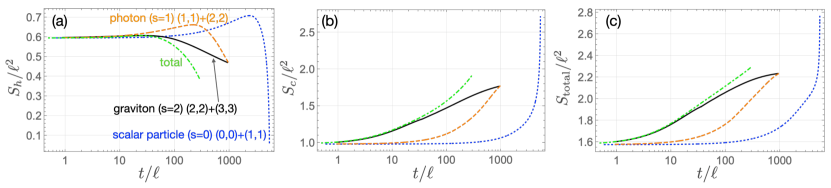
Figure 15: The time-development of the Bekenstein-Hawking entropies, $S_{\rm h}$, $S_{\rm c}$, and $S_{\rm total}$, are shown. We set the same initial condition as in figure 13.

5 Conclusion

In this paper, we computed the time evolution of a KdS black hole formed from gravitational collapse in de Sitter space. We argued for a particular choice of vacuum state that was consistent with the absence of the past cosmological horizon, and applicable to the inflationary universe scenario. The usual Bunch-Davies vacuum state is transformed by collapse into an excitation of an Unruh-like vacuum state. The Hawking stress-energy flux causes the black hole mass and rotation to decay, but has no effect on the cosmological constant.

We derived the spectrum of the energy flux based on these assumptions and computed the greybody factor of the radiation using analytic solutions of the Teukolsky equations on the KdS background. Note that the Teukolsky equations for a massless scalar field reduce to Heun’s equation, but only when it is conformally coupled to gravity. For this reason we have taken the massless scalar field in our analysis to be conformally coupled to gravity. The scalar field (which has a zero angular momentum mode) contributes most of the mass-loss rate at lower black hole spins, while the graviton significantly contributes to mass-loss and spin-loss rates for a rapidly spinning black hole. The rapidly spinning case is dominated by superradiance around the KdS black hole, but the superradiance is weakened by a large value of cosmological constant. We have computed numerically the time evolution of a KdS black hole taking into account dominant modes of scalar, electromagnetic, and gravitational perturbations. In this paper, for simplicity we considered bosonic particles only, leaving fermions for future work. We found, like in the asymptotically flat case, that a rotating black hole in de Sitter space loses angular momentum faster than it loses mass. We also argued that there are no black holes which evolve toward the Nariai limit.

We have also computed the horizon entropy and have found that the generalized second law of thermodynamics still holds thanks to the cosmological constant, at least within the parameter region we have investigated numerically. Knowledge of the heat fluxes raises the possibility of combining this with concepts from non-equilibrium thermodynamics. For example, at a linearized level we might take interacting fields and study the transport properties of the medium between the horizons, taking into account heat flows and entropy production for the interacting fluxes. It would also be interesting to explore the similarities to those systems with evolving heat fluxes in extended irreversible thermodynamics Jou, Casas-Vazquez, and Lebon (1988).

Appendix A Normalisation

We will explain here the normalisation of the modes given in Eq. (19) for the expansion (14). The norm of a state is defined by Unruh (1974),

$$\langle\phi,\phi\rangle=i\int_{\Sigma}\sqrt{-|g|}g^{t\mu}(\phi\,\phi^{*}_{,\mu}-\phi_{,\mu}\phi^{*})d^{3}x,$$ (112)

where $\Sigma$ is a constant time surface. The various contribution are,

$$\sqrt{-|g|}={\rho^{2}\sin\theta\over\Xi},$$ (113)

and close to the horizons,

$$g^{t\mu}\partial_{\mu}\to-{(a^{2}+r^{2})^{2}\over\Delta_{r}\rho}\hat{\partial}_{t}$$ (114)

where $\hat{\partial}_{t}=\partial_{t}-\Omega\partial_{\varphi}$. Finally,

$$drd\theta d\varphi={\Delta_{r}\over a^{2}+r^{2}}dr^{*}d\theta d\varphi$$ (115)

Hence, near the horizons,

$$\langle\phi,\phi\rangle=-i\int{a^{2}+r^{2}\over\Xi}(\phi\hat{\partial}_{t}\phi^{*}-\hat{\partial}_{t}\phi\,\phi^{*})\sin\theta\,dr^{*}d\theta d\varphi.$$ (116)

To normalise, we insert the expansion of $\phi$ for two generic modes,

$$\begin{split}\langle\phi_{\omega lm_{z}},\phi_{\omega^{\prime}l^{\prime}m_{z}^{\prime}}\rangle=&\ \frac{2\pi}{\Xi}\delta_{m_{z}m_{z}^{\prime}}(\omega_{c,h}+\omega^{\prime}_{c,h})e^{-i(\omega-\omega^{\prime})t}\\ &\ \ \times\int d\theta\sin\theta S_{\omega lm_{z}}S_{\omega^{\prime}l^{\prime}m_{z}^{\prime}}\int dr_{*}R_{\omega lm_{z}}R^{*}_{\omega^{\prime}l^{\prime}m_{z}^{\prime}}.\end{split}$$ (117)

By constructing wave packets in the region containing the incident part of the wave, we can substitute ${\overleftarrow{R}}_{\omega lm_{z}}=\mathcal{N}_{c}e^{-i\omega_{c}r_{*}}$ at $r=r_{c}$ and ${\overrightarrow{R}}_{\omega lm_{z}}=\mathcal{N}_{h}e^{i\omega_{h}r_{*}}$ at $r=r_{h}$, where $\mathcal{N}_{c,h}$ are the normalisation factors to be found. The integral in $r_{*}$ then becomes $|\mathcal{N}_{c,h}|^{2}\delta_{\omega\omega^{\prime}}$ and the angular functions are normalised such that the $\theta$ integral becomes $(2\pi)^{-1}$ for the same $l$ mode. Thus, we find $\mathcal{N}_{c,h}=\sqrt{\Xi/|2\omega_{c,h}|}$ as claimed in (19).

Appendix B Blueshifted flux in the Nariai limit and its finiteness

We investigate the behaviour of the spectra $d^{2}M/dt/d\omega$ and $d^{2}J/dt/d\omega$ in the Nariai limit and show that the flux measured by an observer in the region between the black hole and cosmological horizon is still finite value even in the Nariai limit. The spectra shown in (108) and (109) can be approximated as follow in the Nariai limit and $\omega<m_{z}\Omega_{c}(\omega_{c}<0)$:

$$\begin{split}\frac{d^{2}M}{dtd\omega}&=\frac{1}{2\pi}(\omega+am_{z}/\ell^{2}){}_{s}\Gamma_{\omega lm_{z}}\frac{1}{2}\left\{\coth{\left(\frac{\beta_{h}\omega_{h}}{2}\right)}-\coth{\left(\frac{\beta_{c}\omega_{c}}{2}\right)}\right\}\\ &=\frac{1}{4\pi}(\omega+am_{z}/\ell^{2}){}_{s}\Gamma_{\omega lm_{z}}\left(-\frac{1+\exp(\beta_{h}\omega_{h})}{1-\exp(\beta_{h}\omega_{h})}+\frac{1+\exp(\beta_{c}\omega_{c})}{1-\exp(\beta_{c}\omega_{c})}\right)\\ &\simeq\frac{1}{2\pi}(\omega+am_{z}/\ell^{2}){}_{s}\Gamma_{\omega lm_{z}}\left(\exp(\beta_{c}\omega_{c})-\exp(\beta_{h}\omega_{h})\right)\to 0,\end{split}$$ (118)

where we used $\beta_{h},\beta_{c}\to\infty$ in the Nariai limit. From this estimation, one can conclude that $d^{2}J/dt/d\omega$ is also exponentially suppressed in $\omega<m_{z}\Omega_{c}$. When $\omega>m_{z}\Omega_{h}$, we have

$$\begin{split}\frac{d^{2}M}{dtd\omega}&=\frac{1}{2\pi}(\omega+am_{z}/\ell^{2}){}_{s}\Gamma_{\omega lm_{z}}\frac{1}{2}\left\{\coth{\left(\frac{\beta_{h}\omega_{h}}{2}\right)}-\coth{\left(\frac{\beta_{c}\omega_{c}}{2}\right)}\right\}\\ &=\frac{1}{4\pi}(\omega+am_{z}/\ell^{2}){}_{s}\Gamma_{\omega lm_{z}}\left(\frac{1+\exp(-\beta_{h}\omega_{h})}{1-\exp(-\beta_{h}\omega_{h})}-\frac{1+\exp(-\beta_{c}\omega_{c})}{1-\exp(-\beta_{c}\omega_{c})}\right)\\ &\simeq\frac{1}{2\pi}(\omega+am_{z}/\ell^{2}){}_{s}\Gamma_{\omega lm_{z}}\left(\exp(-\beta_{h}\omega_{h})-\exp(-\beta_{c}\omega_{c})\right)\to 0,\end{split}$$ (119)

from which we also have $d^{2}J/dt/d\omega\to 0$ for $\omega>m_{z}\Omega_{h}$ in the Nariai limit.

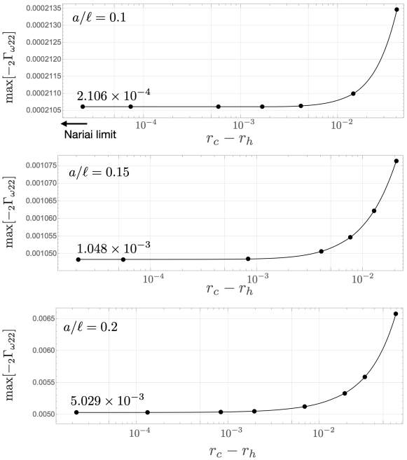
Figure 16: The maximum values of the greybody factor for graviton ($s=2$) with $(l,m_{z})=(2,2)$ near the Nariai solution for $a/\ell=0.1$, $0.15$, and $0.2$.

Let us next consider the superradiant frequencies, $m_{z}\Omega_{c}<\omega<m_{z}\Omega_{h}$, in the Nariai limit. The spectrum is

$$\begin{split}\frac{d^{2}M}{dtd\omega}&=\frac{1}{2\pi}(\omega+am_{z}/\ell^{2}){}_{s}\Gamma_{\omega lm_{z}}\frac{1}{2}\left\{\coth{\left(\frac{\beta_{h}\omega_{h}}{2}\right)}-\coth{\left(\frac{\beta_{c}\omega_{c}}{2}\right)}\right\},\\ &=\frac{1}{4\pi}(\omega+am_{z}/\ell^{2}){}_{s}\Gamma_{\omega lm_{z}}\left(\frac{2}{\beta_{h}\omega_{h}}-\frac{2}{\beta_{c}\omega_{c}}\right),\\ &\simeq-\frac{1}{2\pi}(\omega+am_{z}/\ell^{2}){}_{s}\Gamma_{\omega lm_{z}}\beta_{h}^{-1}\frac{1}{k(1-k)}\frac{1}{\Delta\omega}\propto(r_{c}-r_{h})^{0},\end{split}$$ (120)

where $\Delta\omega\equiv m_{z}(\Omega_{h}-\Omega_{c})$ and we set $\omega=m_{z}\Omega_{c}+k\Delta\omega$ with $0<k<1$. Since both $\beta_{h}^{-1}$ and $\Delta\omega$ are proportional to $(r_{c}-r_{h})$, the spectrum amplitude is still finite and non-zero even in the Nariai limit for the superradiant frequencies. Then we found out that $dM/dt$ and $dJ/dt$ are proportional to $\Delta\omega\propto r_{c}-r_{h}$.

An observer in the region between the horizons measures $dM/d\tau=(dt/d\tau)dM/dt$ and $dJ/d\tau=(dt/d\tau)dJ/dt$, where $\tau$ is the proper time of the observer. The factor $dt/d\tau$ has the blueshift factor $1/\sqrt{\Delta_{r}}$ which enhances the intensity of flux by $\sim 1/(r_{c}-r_{h})$ in the Nariai limit. Therefore, the gravitational blueshift cancels the suppression of $(r_{c}-r_{h})$ in $dM/dt$ and $dJ/dt$, and in general, the measured fluxes $dM/d\tau$ and $dJ/d\tau$ are still finite and non-zero, even in the Nariai limit.

Note that $1/k(k-1)$ in (120) does not lead to the divergence of $d^{2}M/dt/d\omega$ at $\omega\to m_{z}\Omega_{c/h}$ because the greybody factor ${}_{s}\Gamma_{\omega lm_{z}}$ suppresses the flux with the power of $(\omega-m_{z}\Omega_{c/h})$. Also, the greybody factor has its positive value even in the Nariai limit for superradiant frequencies and the maximum values of greybody factor for fixed spin parameters are shown in figure 16.

Finally, let us evaluate $dM/d\tau$ in the non-spinning Nariai limit. When $a=0$, the energy flux is

$$\begin{split}\frac{dM}{dt}&=\int_{0}^{\infty}d\omega\frac{\omega}{2\pi}{}_{s}\Gamma_{\omega lm_{z}}\frac{1}{2}\left\{\coth{\left(\frac{\beta_{h}\omega}{2}\right)}-\coth{\left(\frac{\beta_{c}\omega}{2}\right)}\right\}\\ &\simeq\int_{0}^{\infty}d\omega\frac{\omega}{2\pi}{}_{s}\Gamma_{\omega lm_{z}}\left(\exp(-\beta_{h}\omega)-\exp(-\beta_{c}\omega)\right)\\ &\sim\frac{{}_{s}\Gamma_{0lm_{z}}}{2\pi}\int_{0}^{\infty}d\omega\omega\left(\exp(-\beta_{h}\omega)-\exp(-\beta_{c}\omega)\right)\\ &=\frac{{}_{s}\Gamma_{0lm_{z}}}{2\pi}\left(\frac{1}{\beta_{h}^{2}}-\frac{1}{\beta_{c}^{2}}\right)\\ &\simeq\frac{{}_{s}\Gamma_{0lm_{z}}}{2\pi}\frac{2}{\beta_{h}}\left(\frac{1}{\beta_{h}}-\frac{1}{\beta_{c}}\right)\propto(r_{c}-r_{h})^{3},\end{split}$$ (121)

where we assumed a special situation where $\displaystyle\lim_{\omega\to 0}|{}_{s}\Gamma_{\omega lm_{z}}|>0$ Kanti, Grain, and Barrau (2005); Kanti, Pappas, and Pappas (2014) although the greybody factor is suppressed by a power of $\omega$ in most cases, which increases the power of $(r_{c}-r_{h})$ in the last line of (121). Therefore, taking into account the blueshift factor $\sim 1/(r_{c}-r_{h})$, we have $dM/d\tau\propto(r_{c}-r_{h})^{2}$ which means that it goes to zero in the Nariai limit.

References

- Hawking (1974) S. Hawking, Nature 248, 30 (1974).
- Hawking (1975) S. Hawking, Commun. Math. Phys. 43, 199 (1975), [Erratum: Commun.Math.Phys. 46, 206 (1976)].
- Page (1976a) D. N. Page, Phys. Rev. D 13, 198 (1976a).
- Page (1976b) D. N. Page, Phys. Rev. D 14, 3260 (1976b).
- Candelas (1980) P. Candelas, Phys. Rev. D 21, 2185 (1980).
- Levi and Ori (2015) A. Levi and A. Ori, Phys. Rev. D 91, 104028 (2015), arXiv:1503.02810 [gr-qc] .
- Levi (2017) A. Levi, Phys. Rev. D 95, 025007 (2017), arXiv:1611.05889 [gr-qc] .
- Levi et al. (2017) A. Levi, E. Eilon, A. Ori, and M. van de Meent, Phys. Rev. Lett. 118, 141102 (2017), arXiv:1610.04848 [gr-qc] .
- Unruh (1976) W. G. Unruh, Phys. Rev. D 14, 870 (1976).
- Gibbons and Hawking (1977) G. W. Gibbons and S. W. Hawking, Phys. Rev. D 15, 2738 (1977).
- Qiu and Traschen (2020) Y. Qiu and J. Traschen, Class. Quant. Grav. 37, 135012 (2020), arXiv:1908.02737 [hep-th] .
- Anderson and Traschen (2020) P. Anderson and J. Traschen, “Horizons and Correlation Functions in 2D Schwarzschild-de Sitter Spacetime,” (2020), arXiv:2012.08494 [hep-th] .
- Aalsma, Parikh, and Van Der Schaar (2019) L. Aalsma, M. Parikh, and J. P. Van Der Schaar, JHEP 11, 136 (2019), arXiv:1905.02714 [hep-th] .
- Gong and Seo (2020) J.-O. Gong and M.-S. Seo, “Instability of de Sitter space under thermal radiation in different vacua,” (2020), arXiv:2011.01794 [hep-th] .
- Kay and Wald (1991) B. S. Kay and R. M. Wald, Physics Reports 207, 49 (1991).
- Bunch and Davies (1978) T. S. Bunch and P. C. W. Davies, Proc. R. Soc. Lond. A360, 117 (1978).
- Mellor and Moss (1990) F. Mellor and I. Moss, Phys. Rev. D 41, 403 (1990).
- Chambers and Moss (1994a) C. M. Chambers and I. G. Moss, Phys. Rev. Lett. 73, 617 (1994a), arXiv:gr-qc/9406036 .
- Unruh (1974) W. G. Unruh, Phys. Rev. D 10, 3194 (1974).
- Henneaux and Teitelboim (1985) M. Henneaux and C. Teitelboim, Commun. Math. Phys. 98, 391 (1985).
- Dolan et al. (2013) B. P. Dolan, D. Kastor, D. Kubiznak, R. B. Mann, and J. Traschen, Phys. Rev. D 87, 104017 (2013), arXiv:1301.5926 [hep-th] .
- Dolan (2019) B. P. Dolan, Class. Quant. Grav. 36, 077001 (2019), arXiv:1808.09081 [gr-qc] .
- Chambers and Moss (1994b) C. M. Chambers and I. G. Moss, Class. Quant. Grav. 11, 1035 (1994b), arXiv:gr-qc/9404015 .
- Tachizawa and Maeda (1992) T. Tachizawa and K.-i. Maeda, “Superradiance in the Kerr-de Sitter space-time,” (1992), WU-AP-22-92 .
- Mottola (1985) E. Mottola, Phys. Rev. D 31, 754 (1985).
- Abramo, Brandenberger, and Mukhanov (1997) L. W. Abramo, R. H. Brandenberger, and V. F. Mukhanov, Phys. Rev. D 56, 3248 (1997), arXiv:gr-qc/9704037 .
- Anderson and Mottola (2014) P. R. Anderson and E. Mottola, Phys. Rev. D 89, 104038 (2014), arXiv:1310.0030 [gr-qc] .
- Markkanen (2016) T. Markkanen, JCAP 11, 026 (2016), arXiv:1609.01738 [hep-th] .
- Suzuki, Takasugi, and Umetsu (1998) H. Suzuki, E. Takasugi, and H. Umetsu, Prog. Theor. Phys. 100, 491 (1998), arXiv:gr-qc/9805064 .
- Hatsuda (2020) Y. Hatsuda, Class. Quant. Grav. 38, 025015 (2020), arXiv:2006.08957 [gr-qc] .
- Novaes et al. (2019) F. Novaes, C. Marinho, M. Lencsés, and M. Casals, JHEP 05, 033 (2019), arXiv:1811.11912 [gr-qc] .
- Teukolsky and Press (1974) S. A. Teukolsky and W. H. Press, The Astrophysical Journal 193, 443 (1974).
- Chandrasekhar (1985) S. Chandrasekhar, The mathematical theory of black holes (1985).
- Suzuki, Takasugi, and Umetsu (2000) H. Suzuki, E. Takasugi, and H. Umetsu, Prog. Theor. Phys. 103, 723 (2000), arXiv:gr-qc/9911079 .
- Rosa (2017) J. G. Rosa, Phys. Rev. D 95, 064017 (2017), arXiv:1612.01826 [gr-qc] .
- Jou, Casas-Vazquez, and Lebon (1988) D. Jou, J. Casas-Vazquez, and G. Lebon, Reports on Progress in Physics 51, 1105 (1988).
- Kanti, Grain, and Barrau (2005) P. Kanti, J. Grain, and A. Barrau, Phys. Rev. D 71, 104002 (2005), arXiv:hep-th/0501148 .
- Kanti, Pappas, and Pappas (2014) P. Kanti, T. Pappas, and N. Pappas, Phys. Rev. D 90, 124077 (2014), arXiv:1409.8664 [hep-th] .