Excitation mechanisms in the intracluster filaments surrounding Brightest Cluster Galaxies

Abstract

Context. The excitation of the filamentary gas structures surrounding giant elliptical galaxies at the center of cool-core clusters, a.k.a BCGs (brightest cluster galaxies), is key to our understanding of active galactic nucleus (AGN) feedback, and of the impact of environmental and local effects on star formation.

Aims. We investigate the contribution of the thermal radiation from the cooling flow surrounding BCGs to the excitation of the filaments. We explore the effects of small levels of extra-heating (turbulence), and of metallicity, on the optical and infrared lines.

Methods. Using the Cloudy code, we model the photoionization and photodissociation of a slab of gas of optical depth A${}_{V}\leq$30 mag at constant pressure, in order to calculate self-consistently all of the gas phases, from ionized gas to molecular gas. The ionizing source is the extreme ultraviolet (EUV) and soft X-ray radiation emitted by the cooling gas. We test these models comparing their predictions to the rich multi-wavelength observations, from optical to submillimeter, now achieved in cool core cluster.

Results. Such models of self-irradiated clouds, when reaching large enough A_V, lead to a cloud structure with ionized, atomic and molecular gas phases. These models reproduce most of the multi-wavelength spectra observed in the nebulae surrounding the BCGs, not only the LINER-like optical diagnostics: [O iii]$\lambda$ 5007 $\AA$/H${\beta}$, [N ii]$\lambda$ 6583 Å/H${\alpha}$ and ([S ii]$\lambda$ 6716 $\AA$+[S ii]$\lambda$ 6731 $\AA$)/H${\alpha}$ but also the infrared emission lines from the atomic gas. [O i]$\lambda$ 6300 $\AA$/H${\alpha}$, instead, is overestimated across the full parameter space, except for very low A_V. The modeled ro-vib H₂  lines also match observations, which indicates that near and mid-IR H₂  lines are mostly excited by collisions between H₂  molecules and secondary electrons produced naturally inside the cloud by the interaction between the X-rays and the cold gas in the filament. However, there is still some tension between ionized and molecular line tracers (i.e. CO), which requires to optimize the cloud structure and the density of the molecular zone. The limited range of parameters over which predictions match observations allows us to constrain, in spite of degeneracies in the parameter space, the intensity of X-ray radiation bathing filaments, as well as some of their physical properties like A_V  or the level of turbulent heating rate.

Conclusions. The reprocessing of the EUV and X-ray radiation from the plasma cooling is an important powering source of line emission from filaments surrounding BCGs. Cloudy self-irradiated X-ray excitation models, coupled with a small level of turbulent heating, manage to reproduce simultaneously a large number of optical-to-infrared line ratios when all the gas phases (from ionized to molecular) are modelled self-consistently. Releasing some of the simplifications of our model, like the constant pressure, or adding the radiation fields from the AGN and stars, as well as a combination of matter- and radiation-bounded cloud distribution, should improve the predictions of line emission from the different gas phases.

1 Introduction

X-ray observations of galaxy clusters show that for more than one third of the clusters, the X-ray surface brightness peaks in the center. This emission is due to the cooling of the hot intracluster medium (ICM) with a short radiative cooling time. At the center of these “cool-core” clusters lies a giant elliptical galaxy, the brightest cluster galaxy (BCG). Chandra and XMM-Newton X-ray observations of the BCGs, revealed huge ICM cavities, produced by the jet of the central black hole (e.g., McNamara & Nulsen 2007; Fabian et al. 2015). These cavities highlight the impact of active galactic nucleus (AGN) on their large-scale environments and suggest that the necessary heating source to prevent the overcooling in the cool-core cluster could be provided by the AGN. Observations at different wavelengths of these regions, show that the cavities are often surrounded by multi-wavelength line-emitting filamentary structures (e.g., Heckman et al. 1989; Conselice et al. 2001; Lim et al. 2012; Mittal et al. 2012; Rose et al. 2020), illustrating the multi-phase nature of these streams. Studies of the correlation between H$\alpha$ and CO(1-0) line emission (e.g. Salomé et al. 2011; Tremblay et al. 2018; Olivares et al. 2019; Russell et al. 2019) showed that these two tracers are co-spatial and co-moving with most of the mass of the filaments lying in the molecular phase. These filaments may have formed from the cooling of the hot gas in very local regions around the AGN-cavities, when the gas is locally thermally unstable (e.g. Gaspari et al. 2012; Beckmann et al. 2019; Qiu et al. 2020).

In the last decades several studies have investigated the powering source of the multi-wavelength spectrum of these filamentary nebulae (e.g. Heckman et al. 1989; Voit et al. 1994; Ferland et al. 1994, 2002, 2008; Bayet et al. 2011; Canning et al. 2016), proposing and exploring different sources of photoionization and heating: (1) the central AGN, (2) X-rays from ICM, (3) heat conduction from the ICM to the cold filament, (4) shocks and turbulent mixing layers, (5) collisional heating by cosmic rays, (6) hybrid models (several energy sources). Some of these sources have already been excluded: photoionization by the AGN is not powerful enough to produced the observed H$\alpha$+[N ii] line emission (e.g. Heckman et al. 1989; Conselice et al. 2001) and disagree with the lack of strong radial gradients profile in the optical emission line ratios (e.g. Heckman et al. 1989). The fairly constant H$\alpha$/H₂ (Lim et al. 2012) and H$\alpha$/CO (e.g. Olivares et al. 2019) over the entire nebula, also suggests that the excitation process is local. A local ionization mechanism could be the photoionization by young massive stars, but this scenario is not favored either, since the observations show strong [N ii]$\lambda$ 6583 Å/H${\alpha}$ ratio and weak [O iii]$\lambda$ 5007 $\AA$/H${\beta}$ ratio, indicating that the optical spectra of these nebulae are more similar to low ionization nuclear emission region (LINER) spectra than HII  spectra (e.g. Heckman 1987; Crawford & Fabian 1992). Mcdonald et al. (2012) claimed that a model with a mix of heating by shocks (100 - 400 km s^-1; Allen et al. 2008) and photoionization by stars (Kewley et al. 2001) can reproduce the optical line ratios [N ii]$\lambda$ 6583 Å/H${\alpha}$, [O i]$\lambda$ 6300 $\AA$/H${\alpha}$, ([S ii]$\lambda$ 6716 $\AA$+[S ii]$\lambda$ 6731 $\AA$)/H${\alpha}$, and [O iii]$\lambda$ 5007 $\AA$/H${\beta}$, of a sample of nine BCGs. But this study was limited to optical lines only. In the near infrared, Jaffe & Bremer (1997) investigated the line ratio H₂ 1-0 S(1)/H$\alpha$. They measured a ratio of $\sim$0.1, which is larger than the observed ratio in Galactic HII  regions ($\sim$0.01) and excludes fast shocks (¿50 km s^-1) as possible excitation mechanism. The possible source of excitation of the ro-vibrationally excited H₂ lines in the filaments have been discussed also by Wilman et al. (2002) and Lim et al. (2012).

Focusing on one filament around NGC 1275, the so-called Horseshoe-region, Ferland et al. (2008, 2009) extended the observational constraints from optical to infrared, and proposed as the main heating mechanism, the collisions of the cold gas in the filaments with ionizing particles. The authors showed that this model is consistent with the filaments being made of cloudlets of varying densities and excited by cosmic-rays. One strong motivation and success of this model was to reproduce the surprisingly strong molecular hydrogen lines detected by Spitzer in Perseus and Centaurus filaments (Johnstone et al. 2007), together with the ratios of the near infrared (NIR) H₂ line emission, as well as the lack of [O iii]$\lambda$ 5007 $\AA$  emission line noticed in most of the filaments of Perseus by Hatch et al. (2006). Fabian et al. (2011) showed that the surrounding hot ICM is a possible source of these energetic particles. Bayet et al. (2011) used the same kind of model (energetic particles with/without extra-heating) to predict molecular emission lines like CN (2–1), HCO⁺ (3–2) and C₂H (3–2). With the advent of Herschel Space Observatory, the detection of the far-infrared (FIR) [C ii]$\lambda$ 157.7 $\mu$m  and [O i]$\lambda$ 63.2 $\mu$m  line emission, was made possible in BCGs and even mapped in the filaments of the Perseus and Centaurus clusters. Mittal et al. (2012) showed that the observed ratio [O i]$\lambda$ 63.2 $\mu$m/[C ii]$\lambda$ 157.7 $\mu$m was barely reproduced by the energetic particles model only. In order to reproduce this ratio with such model, it is necessary to add an extra heating source such as turbulent heating, with typical velocity dispersion of 2-10 km s^-1as shown in Canning et al. (2016). This model succeed on reproducing the observations, however, it is a result of a weighted sum of a power-law distribution of cloud densities for which the Cloudy computation was stopped at the illuminated face of the cloud (first zone), i.e. only emission from the skin of the clouds was combined. In Canning et al. (2016) the authors investigated the behavior of the predicted line emissivity throughout a cloud at fixed density, but not for an integral of clouds of many densities.

In this paper we re-investigate the effect of the excitation due to thermal radiation as expected from the cooling of the hot plasma and we explore the outcomes due to photoionization at different depth of the cloud, namely the visual extinction (A_V). The photoionization by the X-ray photons emitted by the condensing and cooling gas, the so-called cooling flow, was already considered (i.e. Voit & Donahue 1990; Ferland et al. 1994; Donahue & Voit 1991 and references therein). The cool-core clusters have measured mass deposition rates of 10 - 100 M_⊙ yr^-1, or smaller when considering regions inside the filaments. Even if large amount of energy are expected via this cooling gas, Crawford & Fabian (1992) argued against this process to power the nebula. From unresolved X-ray data, they showed that the photoionization by the surrounding X-ray gas was not powerful enough to excite the nebula of the core of the Perseus cluster. Recent deep and high resolution observations of X-ray filaments by the satellite Chandra (Walker et al. 2015) show an average intensity of twelve filaments in Perseus of 4$\times$10^-16 erg cm^-2 s^-1arcsec^-2, made this mechanism interesting to explore again. In the present study, we do not add any other source of excitation in order to measure and discuss the effects of reprocessing the X-ray cooling energy from the ionized to the molecular phase. We are aware that this model is over-simplified to be able to reproduce all of the gas phases simultaneously. We emphasize that we explore the physical properties of the cloud and the predicted line emission at different A_V. We also discuss the impact of adding some turbulent heating and of varying the metallicity (Z) on the physical and chemical properties of the cloud. We compare model predictions with observations of line emission from the filaments, combining the state-of-the-art models with the recent observations at different wavelengths, from the optical to the infrared, extending the range of constraints and predictions for a single model.

The model setup is described in section 2.1. The effects on varying the different free parameters are analyzed in sections 2.2 and  2.3. The predicted optical-to-submillimeter line emission from our grid of models are compared with the observations provided by the literature in section 3. Our results are discussed in section 4 and the conclusions are summarized in section 5.

2 Modeling

In this section we present the setup of the Cloudy  models as well as the evolution of the chemical and physical structure of the cloud with the free parameters of the models.

2.1 Setup of the models

We use the photoionization and photodissociation code Cloudy v17.01 (Ferland et al. 2017), which allows to calculate self-consistently the thermal and chemical structure of a plane-parallel layer of a gas and dust. Previous studies focused the analysis on the neutral and molecular phases, however, the initial conditions of each phase are a consequence of the processes that take place on the previous phase. Moreover, some line emission, such as [C ii]$\lambda$ 157.7 $\mu$m, can arise from both ionized and neutral phase. Hence, computations that do not take into account multiple gas phases could bring incorrect interpretation to the phase properties. In our analysis, each model is performed at a constant total pressure of 10^6.5 K cm^-3, which is the average pressure of the hot gas surrounding the filaments of NGC 1275, as deduced from X-ray observations (Sanders & Fabian 2007). Similar pressure values have been estimated from the electron density calculated with the line ratio [S ii]$\lambda\lambda$ 6716,6731 $\AA$ (e.g. Heckman et al. 1989). All models are stopped at the visual extinction of A_V = 30 mag. Other input parameters for the models are: the shape and intensity of the incident radiation field, the chemical composition of dust and gas, the metallicity (Z) and the turbulent velocity dispersion (v_tur). A_V = 30 mag correspond to slightly different physical size, based on the initial conditions of the model. To give an order of magnitude, for a model of G_X =10, v_tur=10 km s^-1  and Z = Z_⊙ the size of the full cloud is $\sim$48 pc. The model parameters are described in detail below and a summary is provided in Table 1.

Table 1: Model summary.

Fixed parameters
Geometry	1D plane-parallel
Radiation field	intergalactic background continuum
	HM05a at redshift 0
	Table SED “cool.sed”(d) (X-ray emission), intensity (GXc) set to values below
	ISRFb scaled to G${}_{0}^{c}$=10-5
	CMB
	cosmic ray background: H0 ionization rate of 2$\times$10-16 s-1
Density law	constant pressure set to 106.5 K cm-3
Varied parameters	values
X-ray radiation field intensity (GX)	[10-2, 10-1.8, 10-1.6, 10-1.4, 10-1.2, 10-1, 10-0.8, 10-0.6, 10-0.4, 10-0.2, 1, 10, 101.2, 101.4, 101.6 , 101.8, 102, 102.2, 102.4, 102.6, 102.8, 103]
Metal abundances (Z)	[0.3, 0.35, 0.4, 0.45, 0.5, 0.55, 0.6, 0.65, 0.7, 0.75, 0.8, 0.85, 0.9, 0.95, 1] Z⊙
Turbulent velocity (vtur)	[0, 2, 10, 30, 50, 100] km s-1

Notes. ^(a) Haardt $\&$ Madau radiation field available in Cloudy. ^(b)Interstellar radiation field calculated by Meudon PDR code (Le Petit et al. 2006) using the radiation field from Mathis et al. (1983). ^(c)G_X = 1 (respectively G₀ = 1) corresponds to an integrated intensity between 0.2 and 2 keV (respectively 6 - 13.6 eV) of 1.6$\times$10^-3erg cm^-2 s^-1. ^(d)SED shape available in Cloudy  to reproduce an X-ray emission from cooling flow gas.

2.1.1 Input radiation field: shape

One of the key parameters of the present modeling is the shape of the input radiation field. Energetic particles or hard X-ray fail to reproduce the observed [O iii]$\lambda$ 5007 $\AA$/H${\beta}$  ratio, because they produce too low highly ionized oxygen [O iii]$\lambda$ 5007 $\AA$  with respect to the other ionized species. To solve this problem, extreme ultraviolet (EUV) as well as soft X-ray photons are necessary since they manage to create and excite the different ions. The slope of the input field has thus a direct impact on the ionized line ratios. Such photons can be emitted by the gas in cooling flows (self-irradiation). This model has been described in Johnstone et al. (1992). The total emission due to the gas that cools constantly from the temperature of the hot surrounding medium, is the result of the sum of the gas emission at each temperature normalized by the mass deposition rate. In our models, the soft X-ray/EUV band of the input radiation field is thus a power-law resulting by the co-added series of Raymond-Smith collisional-equilibrium continua (Raymond & Smith 1977). This continuum shape is available in Cloudy as an input spectral energy distribution (SED) shape and it has been already used in Ferland et al. (1994, 2002) to model cooling flow environments. Fig. 1 shows that almost all of this soft X-ray, EUV radiation is self-absorbed and reprocessed at larger wavelength when it encounters a cloud with a large enough depth. As explained in section  2.1.2, we fine-tune the input radiation intensity and the A_V  to reproduce the X-ray surface brightness observed in the filaments of Perseus. Our simplified model do not explore the spatial distribution or the size distribution of the clouds. We note that one strong hypothesis of this model is that a large fraction of the hot cooling gas radiation is absorbed and reprocessed by the slab of atomic and molecular gas. Our models explore a range of cloud optical depths, which allows us to both match the observed X-ray fluxes and multi-wavelength line emission. We leave for a further work a more complex model of a fog of atomic and molecular clouds spread in a bath of hot cooling gas.

We also added an intergalactic background continuum, taken to be the 2005 version of the Haardt & Madau (1996) background at redshift 0, with both starburst and quasar continua. The input SED also includes the cosmic microwave background (CMB) and the infrared dust emission of the standard interstellar radiation field.

2.1.2 Input radiation field: intensity

The intensity of the X-ray/EUV emission is varied with the parameter G_X. By definition G_X = 1 corresponds to an integrated intensity between 0.2 - 2 keV of 4$\pi\nu$F$\nu$ = 1.6$\times$10^-3 erg cm^-2s^-1. To compare the input and output values of the radiation field in Cloudy with the observed surface brightness, one has to divide this values by 4$\pi$ in order to get values in erg cm^-2 s^-1 sr^-1. For instance G_X = 1 corresponds to an input field of 1.3$\times$10^-4 erg cm^-2s^-1 sr^-1, that is 3$\times$10^-15 erg cm^-2s^-1 arcsec^-2.

We compared the Cloudy outward radiation field in the range 0.6-2.0 keV with the X-ray surface brightness observed in the same band by Walker et al. (2015) in the filaments of the Perseus cluster. The authors estimated that the average surface brightness in this band of the filaments is 4.0$\times$10^-16 ergs cm^-2 s^-1 arcsec^-2. This is the red dot at 2.1$\times$10^-4 erg cm^-2s^-1 on Fig. 1. To give orders of magnitudes, Sanders et al. (2005) estimated the surface brightness of the hard X-ray emission in the band 2-10 keV and found that it decreases with the radius, from $\sim$5$\times$10^-15 ergs cm^-2 s^-1 arcsec^-2 at radius 20 arcsec (magenta dot on Fig. 1) to 10^-16 ergs cm^-2 s^-1 arcsec^-2 at radius 200 arcsec.

In our grid of models, G_X varies between 10^-2 and 10³, with step of 0.2 dex. Note that the range of G_X that is explored here is higher than in Ferland et al. (1994, 2002) where self-irradiated clouds had also been modeled. The values used at that time were scaled on unresolved X-ray observations. The more recent X-ray observations in Perseus are by Sanders & Fabian (2007); Walker et al. (2015) showed that the X-ray radiation is not homogeneously spread over the entire 100 kpc region and soft X-ray emission arising from the filaments surrounding NGC 1275 have surface brightness values reaching up to a few 10^-16 ergs cm^-2 s^-1 arcsec^-2 as mentioned above. The comparison between the input SED used by Ferland et al. (1994) and the input SED of one of our models is shown in Figure 10. Figure 1 shows that low G_X are too small compared to the X-ray observations in Perseus. We nevertheless include grids of model with such low G_X in order to show the effect of turning-on G_X radiation.

2.1.3 Outward radiation field: cloud optical depth effects

The new aspect of our modeling is that we self-consistently compute the chemical, thermodynamical structure and emissivity of the entire cloud as a function of A_V $\leq 30$ mag. Figure 1 shows how the outward, transmitted spectrum changes with the total A_V  of the cloud. With the increase of A_V, i.e. of the hydrogen column density, the cloud absorbs more continuum in the energy range between X-ray to near-infrared (NIR), all of the hydrogen-ionizing radiation is absorbed and the dust emission in FIR increases. Stopping the calculation at A_V=30 mag implies to go throughout different gas phases.

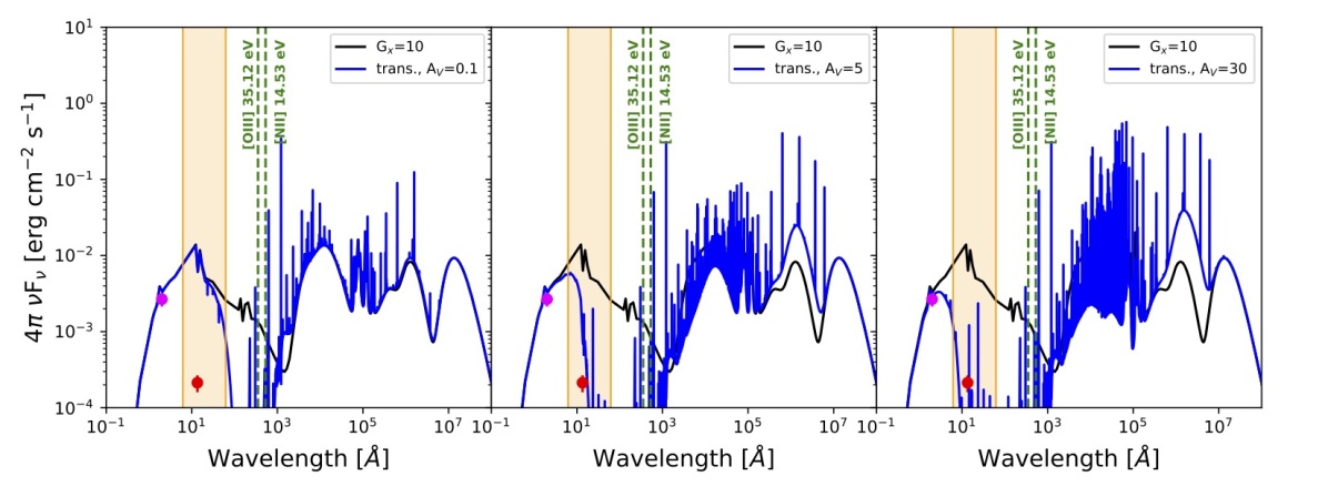
Figure 1: SED of the input radiation field for G_X = 10 (black line) and the total outward radiation field (continuum and line emission) stopping the model at different A_V(blue line): 0.1, 5 and 30 mag. The two vertical green lines show the energy necessary to create the ion O⁺⁺ and N⁺, two of the ions whose emission are used to constrain the modeling. The dots represent the average observed integrated flux for the filaments surrounded NGC 1275 of 4.0$\times$10^-16 erg cm^-2 s^-1arcsec^-2 in the 0.6-2.0 keV band (red dot, Walker et al. 2015), and in the 2-10 keV band (magenta dot) of 5$\times$10^-15 erg cm^-2 s^-1arcsec^-2 (Sanders et al. 2005). The orange background highlights the range over which the integrated intensity is calculated to scale G_X.

2.1.4 Elemental abundances

The chemical setup is based on the previous studies of Ferland et al. (2009) and Canning et al. (2016). The gas elemental abundances and the chemical composition of dust are set to those derived in the Orion Nebula by Baldwin et al. (1991), Rubin et al. (1991), Osterbrock et al. (1992), and Rubin et al. (1993) (see Tables 4 and 5). The grain size distribution is set to the standard distribution in the Milky Way presented in Weingartner & Draine (2001), which consists of a mixture of graphites and silicates and is known to reproduce the standard Galactic extinction curve with $R_{\rm V}$ = 3.1. The polycyclic aromatic hydrocarbon (PAH) size distribution is given by a power law described in Abel et al. (2008).

While most parameters are calibrated with Galactic values, it is important to note that the elemental composition and dust properties in the filaments could be different. Indeed, the average metallicity of the ICM is $\sim$0.3 $Z_{\odot}$. However, and as shown by Sanders & Fabian (2007) (Figure 10), the metallicity of the filaments varies with radius, reaching a maximum at a distance of 40 kpc. In their study the metallicity covers a range between 0.5 to 0.7 $Z_{\odot}$. To investigate in our models the effect of the metallicity on the predicted line emission, which will be compared with the line emission arising from the filaments, we explore here values between 0.3 to 1 $Z_{\odot}$ with a step of 0.05.

2.1.5 Turbulence

The input of mechanical energy in filaments surrounding BCGs originates from various processes such as the cascade of kinetic energy injected at large scales by AGN jets and inflated bubbles (e.g. Revaz et al. 2008; Beckmann et al. 2019), the turbulent mixing between the hot and cold phases (Begelman & Fabian 1990; Banerjee & Sharma 2014; Hillel & Soker 2020), and the collisions between intertwined filaments. All these processes generate small scale turbulence which not only induces pressure fluctuations but may also lead to the propagation of low velocity molecular shocks that could be responsible for bright H₂ emission of filaments (Johnstone et al. 2007; Guillard et al. 2012). In Cloudy, turbulence is modelled through a velocity dispersion parameter v_tur  which acts as a pressure support, an homogeneous heating rate, and a contribution to the line broadening for the radiative transfer. In the collisional ionization models presented in Canning et al. (2016), the authors considered turbulent velocity dispersion of $2-10$ km s^-1, which is enough to decrease the optical depths of the lines and improve the cooling efficiency.

The lines originating from the warm gaseous nebula surrounding NGC 1275 have typical full width at half-maximum (FWHM) ranging between 50 and 200 km s^-1 (Lim et al. 2012). In comparison, a FWHM of $\sim$30 km s^-1 was measured from CO(1-0) in the same region (Salomé et al. 2008). More recently, FWHMs of 100 to 140 km s^-1 were obtained from several emission lines of CO for a sample of various BCGs (Olivares et al. 2019) and FWHMs of 3 to 150 km s^-1 from several molecular absorption lines seen against the bright radio core of Hydra-A Rose et al. (2019, 2020).Whether these line widths originate from the internal velocity dispersion of cold filaments or result from relative motions between filaments is an unsolved issue. In the latter case, the velocity dispersion of the cold components would be intrinsically smaller. To explore all possible scenarios, we extend the range of turbulent velocity dispersion studied by Canning et al. (2016) and adopt values of v_tur between 0 and 100 km s^-1.

2.2 Thermal and ionization profiles

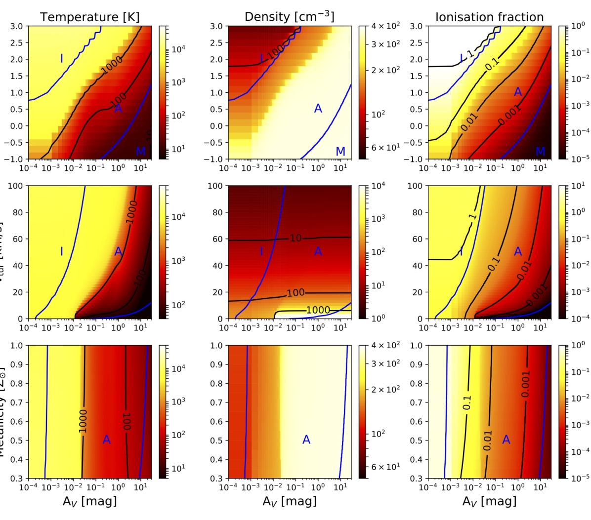
Figure 2: Temperature (left column), hydrogen density (middle column), and ionization fraction $n_{e^{-}}$/$n_{\rm H}$ (right column) of the gas predicted by Cloudy as functions of the visual extinction A_V and the X-ray radiation field scaling factor G_X (top row), the turbulent velocity dispersion v_tur  (middle row), and the metallicity $Z$ (bottom row). Non varying parameters are set to their standard values. In particular the total pressure of the gas is set to 10^6.5 K cm^-3, G_X=10 (for middle and bottom rows), v_tur =10 km s^-1 (for top and bottom rows), and $Z=Z_{\odot}$ (for top and middle rows). The black curves correspond to isocontours. The transition from ionized to atomic phase and that of atomic to molecular defined by $n_{e^{-}}$/$n_{\rm H^{0}}$=1 and to $n_{\rm H^{0}}$/$n_{\rm H_{2}}$=1, respectively, are indicated with a blue curve. The blue I, A and M identify the different gas phases: ionized, atomic and molecular, respectively.

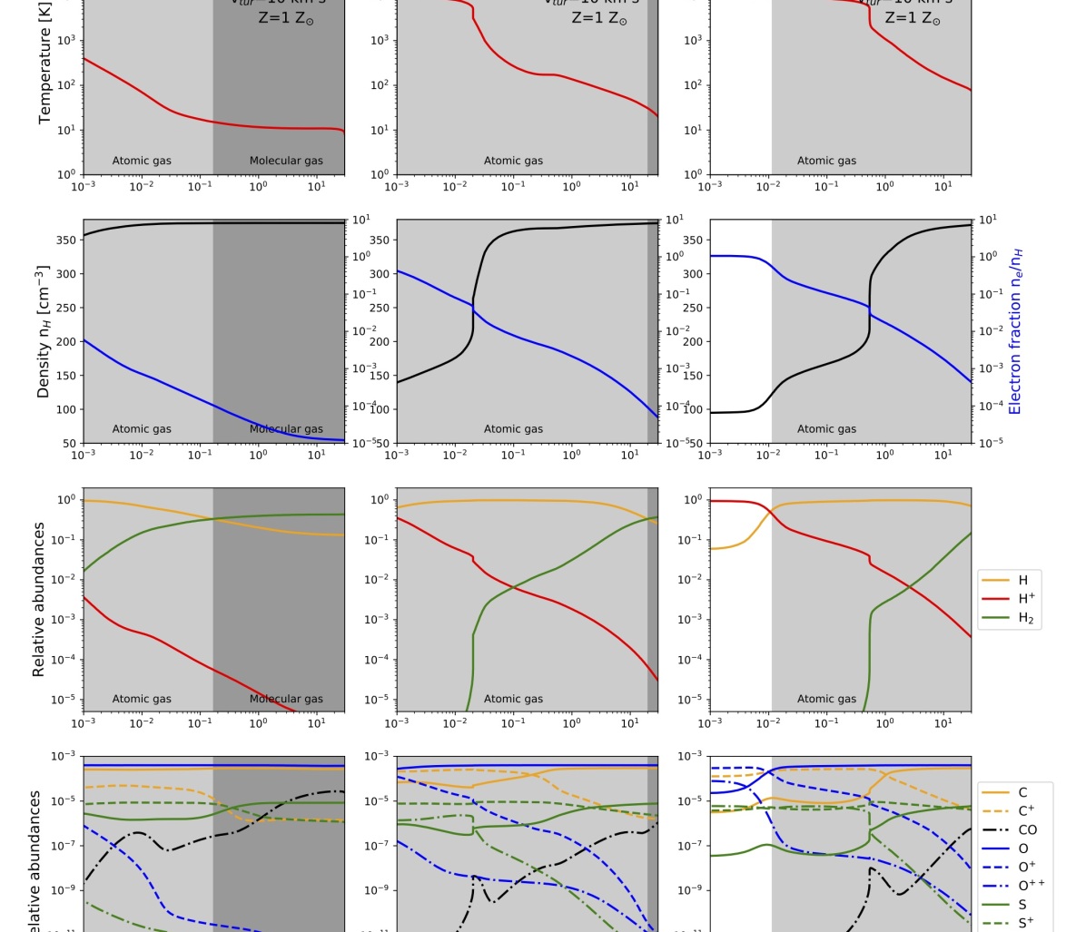
Figure 3: Effects of the radiation field intensity. Physical properties as a function of A_V for models in thermal equilibrium and constant pressure fixed at 10^6.5 K cm^-3, with solar metallicity, turbulent velocity 10 km s^-1 and different values of X-ray radiation field intensity: G_X = 10^-1(left column), G_X = 10¹(central column) and G_X = 10² (right column). Top row: Gas temperatures. Second row: total hydrogen density in black and ionization fraction (n_e/n_H) in blue. Third row: relative abundances of hydrogen. Bottom row: relative abundances of carbon (yellow), oxygen (blue), sulfur (green) and CO (black). The white background indicates the ionized phase, the gray background the atomic phase and the dark gray the molecular phase. The transition from ionized to atomic phase and that of atomic to molecular correspond to density ratio of e^-/H⁰ = 1 and of H⁰/H₂=1, respectively.

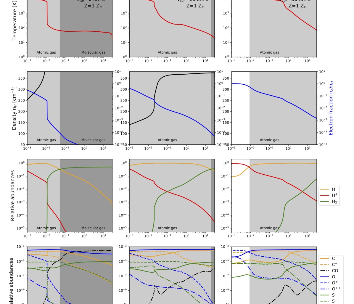
Figure 11: Same as Fig. 3, but this time G_Xis fixed at 10 and the turbulence varies: 0 km s^-1 (left column), 10 km s^-1 (central column) and 50 km s^-1 (right column).

The main parameters of the models are the intensity of the input X-ray radiation field, the turbulence strength, and the metallicity. Figure 2 summarizes how these parameters influence the thermal and ionization structures of a cloud of constant total pressure $P=10^{6.5}$ K cm^-3. To facilitate the interpretation, we also display in Figs. 3, 11, and 13, the main heating and cooling processes, and the chemical profiles associated to seven models representative of the entire parameter domain.

Because X-ray photons dominate both the heating and the ionization rates of the gas, the structures shown in Fig. 2 are similar to the standard profiles predicted in photo-dominated regions (PDRs). As a function of the visual extinction $A_{\rm V}$, the cloud undergoes a transition from a hot ($T\sim 10^{4}$ K), diffuse, and partially or fully ionized phase to a cold ($T\sim 10-100$ K), dense, and partially or fully molecular medium. High temperatures at the border of the cloud result from an equilibrium between the heating induced by photoelectric effect on gas particles and the cooling induced by electronic transitions. In contrast, low temperatures inside the cloud result from a balance between the heating due to photoelectric effect on grains and the cooling induced by fine structure lines and molecular lines. The fact that the photoelectric effect is still efficient at large $A_{\rm V}$ is a known property of X-ray dominated regions (XDRs): because hard X-rays have small interaction cross-sections, they penetrate deep in the cloud where they locally induce the production of UV photons that participate to the ionization of dust and gas, and photodissociation.

The transition between the two thermochemical states is driven by the absorption of the X-ray radiation field. Again, because of the low interaction cross-sections of high energy photons, this transition requires a larger total column density than that required in clouds illuminated only by UV radiation field (Meijerink et al. 2006, 2007). Moreover, because X-rays are mostly absorbed by atoms, self-shielding effects are important. It follows that the cloud structure do not only depend on $A_{\rm V}$ but also on the density profile from the border of the cloud: the smaller the density, the widest the transition. If $G_{\rm X}$ increases, both the ionization and molecular fronts necessarily occur at larger extinction. This is due to the increase of the input X-ray flux at high energy, the decrease of density at the border to ensure a constant total pressure, and the local production of UV photons induced by the thermalization of photoelectrons.

In this framework, the impact of the turbulent velocity dispersion is straightforward. Because the total pressure is assumed to be constant, the mass density is

$$\rho=\frac{P}{\frac{{\rm v}_{\rm tur}^{2}}{2}+\frac{kT}{\mu m_{\rm H}}},$$ (1)

where $P$ is the total pressure, $\mu$ is the mean molecular mass of the gas, and $m_{\rm H}$ the mass of hydrogen atoms. Therefore, the primary effect of the velocity dispersion in Cloudy is to globally reduce the density of the gas over the entire cloud. Equation 1 also reveals a threshold effect: as v_tur  increases, the turbulence pressure (P_tur) increases and the thermal gas pressure (P_th) decreases. When the P_tur becomes higher than the P_th, the cloud switches from a medium at constant thermal pressure with sharp profiles to a medium at constant density with smoother profiles. Such transition occurs for P_tur ¿ P_th, thus

$${\rm v}_{\rm tur}\geqslant{\rm v}_{\rm tur}^{\rm lim}=1.6\,\,\mbox{{\rm km}\,{\rm s}${}^{-1}$}\ \left(\frac{T}{100\,\,{\rm K}}\right)^{0.5}\geqslant 16\,\,\mbox{{\rm km}\,{\rm s}${}^{-1}$},$$ (2)

in agreement with the middle panel of Fig. 2. Finally, since $\rho$ decreases when v_tur  increases, both the ionization and molecular fronts necessarily shift towards larger $A_{\rm V}$.

As shown in Figures 2 and 13, the metallicity appears to have a very limited impact on the thermochemical properties of the cloud. This result is slightly misleading because the metallicity is explored over a narrow range of values. When the metallicity decreases, the abundances of dust and heavy elements decrease by the same factor. A given $A_{\rm V}$ therefore corresponds to higher hydrogen column density, hence the ionization front occurs correspondingly sooner.

2.3 Cumulative emission

The physics of a cloud illuminated by high energy photons is driven by the reprocessing of the input radiation field into continuum and line emission. A PDR (illuminated by UV photons) and an XDR (illuminated X-ray photons) differ by the nature of this reprocessing and the amount of matter it requires. In classical PDRs, the input energy flux is reprocessed over typical visual extinction $A_{\rm V}\sim 1$, mostly through continuum dust emission; only a few percent is converted into atomic and molecular lines. In contrast, and because the impinging radiation field consists of photons of higher energies (X-ray; see Fig. 1), the reprocessing of the input radiative flux in XDRs not only requires large total column densities ($A_{\rm V}$ typically larger than 30 magnitudes), but also occurs through efficient atomic and molecular line emissions.

Following the definitions of Meijerink & Spaans (2005), the X-ray energy flux impinging the cloud is

$$F_{\rm X}=1.6\times 10^{-3}G_{\rm X}\,\,{\rm erg}\,\,{\rm cm}^{-2}\,\,{\rm s}^{-1}.$$ (3)

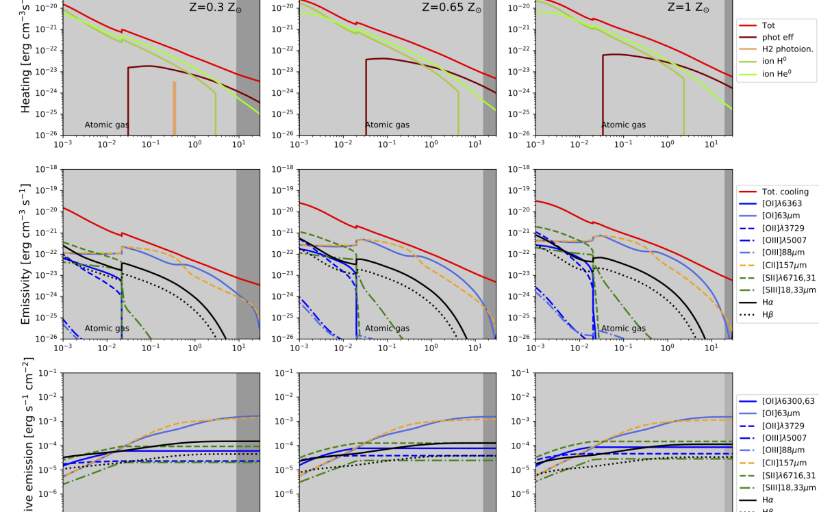
Figure 14: Same as Fig. 4, but this time G_Xis fixed at 10 and the metallicity varies: Z=0.3 Z_⊙ (left column), Z=0.65 Z_⊙ (central column) and Z= Z_⊙ (right column).

The resulting absorption and emission processes are shown in Figs. 4, 12, and 14 where we display the local cooling and the cumulative emissions of fine-structure, metastable, and electronic lines of several atoms and ions for different values of G_X, v_tur  and $Z$.

The excitation of H${\alpha}$ and H${\beta}$ occurs through collisions with high energy secondary electrons and through recombination of H⁺. As a result, the integrated fluxes of these lines are simply proportional to the input radiation field,

$$F({\rm H}\alpha)\sim 10^{-5}G_{\rm X}\,\,{\rm erg}\,\,{\rm cm}^{-2}\,\,{\rm s}^{-1}$$ (4)

and

$$F({\rm H}\beta)\sim 3\times 10^{-6}G_{\rm X}\,\,{\rm erg}\,\,{\rm cm}^{-2}\,\,{\rm s}^{-1},$$ (5)

regardless of the metallicity or the density profile set by v_tur  (Figs. 12 & 14). Because of these simple relations, H${\alpha}$ and H${\beta}$ are valuable proxys of the input radiation field and can thus be used as normalization factors for other atomic and ionized lines. The results of Cloudy on the optical line ratios are presented in Sec. 3.1 where we introduce and discuss the predicted Baldwin–Phillips–Terlevich (BPT) diagrams (Baldwin et al. 1981).

Unlike to H${\alpha}$ and H${\beta}$, the metastable and electronic lines of [S ii], [N ii], and [O iii] are primarily excited by collisions of S⁺, N⁺, and O⁺⁺ with thermalized electrons. Because the excited levels lie at $\sim 2.5\times 10^{4}$ K above the ground state, the corresponding emissivity not only depend on the ionization profiles of the cloud but also on its temperature, and, in particular, on the amount of gas above $\sim 5000$ K. The integrated intensities of all these lines are therefore built up at the border of the cloud where the gas is both ionized and warm. Since the ionization potential of O⁺ is considerably larger than that of O, N, or S, [O iii] lines necessarily trace the outskirt of the [O ii], [N ii], and [S ii] emitting regions. In this framework, the dependencies on the input parameters are straightforward and simply follow the results presented in the previous section. Low density or strong X-ray radiation field naturally favor large abundances of ionized species at the border of the cloud and the depth over which the gas is at high temperature. The integrated intensities of [O ii], [N ii], [S ii], and [O iii] lines therefore increase with $G_{\rm X}$ but also with v_tur  if v_tur$\geqslant$ v_tur^lim (Figs. 4 & 12).

All the lines described above are tracers that carry only a small fraction $\sim 10^{-2}$ of the input X-ray energy flux. Indeed, because of the assumed initial SED, the impinging X-ray radiation field is preferentially reprocessed into the fine structure lines of [O i] and [C ii], providing that $A_{\rm V}$ is sufficiently large. As a result, for most of the models considered here, these lines not only carry a substantial amount of the input radiative flux, but also strongly depend on the size of the cloud. Evidently, the integrated intensities of both [O i] and [C ii] increase with $G_{\rm X}$. The increase of v_tur, instead, has a different effect on the two cooling lines. When v_tur  increases, the density decreases while the temperature increases. For large densities, C+ is converted into C very early in the cloud (see Fig. D1, left), while the transition happens later in a low density medium (see Fig. D1, right). Thus, the integrated intensities of [C ii] increase with v_tur. The integrated intensities of [O i], instead, slightly decrease due to the increasing temperature.

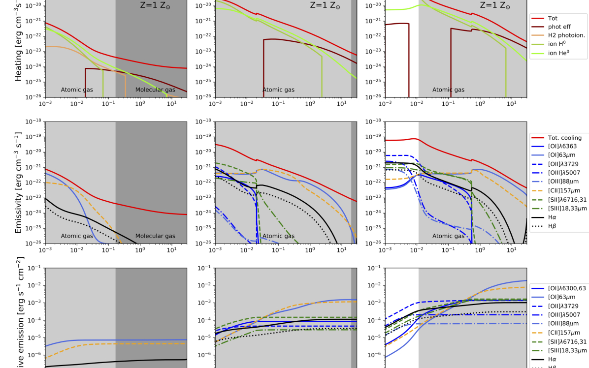
Figure 4: Effects of the radiation field intensity on heating mechanisms and line emission. Heating and cooling mechanisms as a function of A_V for the same models as those in Fig. 3. Top row: heating mechanisms. Cloudy gives in output the first five main heating mechanisms. If one of the heating mechanisms is not one of them for some values of A_V, the mechanism is not shown in the figures. This is the reason of some vertical straight lines in the panels. Second row: emissivity of carbon, oxygen and sulphur lines, H${\alpha}$  and H${\beta}$. Bottom row: cumulative emission of carbon, oxygen and sulphur lines, H${\alpha}$  and H${\beta}$. The cumulative emission are theoretical values, and some of this values are too faint to be detected by the instruments. The instrumental limitations give access only to the brightest values, thus to those emission arising from the denser part of the cloud. It is important to remember that comparing the observations with these predicted line emission we constrain the properties of the denser phase of the cloud.

3 Comparison with the observables

In this section the predicted line emission from our grid of models are compared with the observations, from optical to submillimeter, of several BCGs.

3.1 Optical tracers

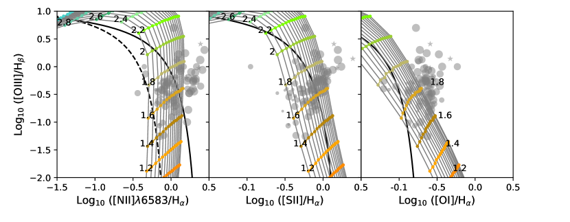
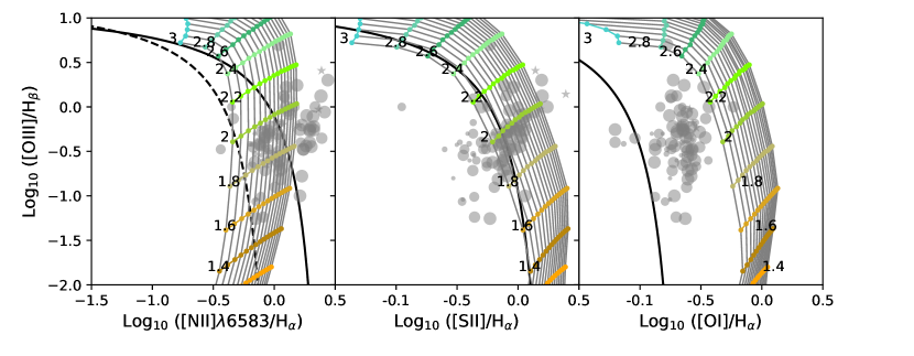
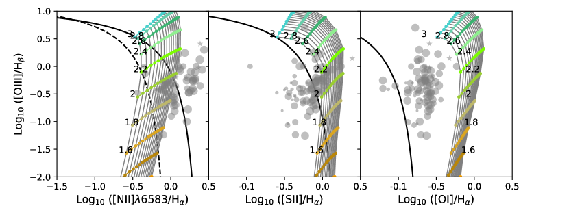
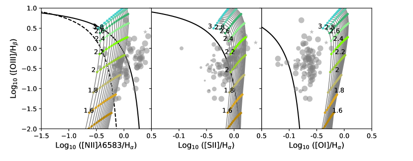
Figure 15: BPT diagrams. Comparison of the observed line ratios with the model predictions. The gray dots (filament values) and the stars (nucleus values) represent the data from Mcdonald et al. (2012). The size of the dots decreases with the increase of the distance from the nuclei of the corresponding object. The solid black line is the upper limit for HII  regions by Kewley et al. (2001) and the dashed black line is the lower limit for AGN by Kauffmann et al. (2003). The predicted cumulative line ratios from the models are overlaid. The gray lines correspond to a single value of metallicity and different values of X-ray emission (the logarithm of the value is written on the left and reproduced with different colours); from left to right the X-ray emission is constant and the metallicity increases (from 0.3 to 1 Z_⊙). The turbulent velocity is fixed to 10 km s^-1. Left column: cumulative emission of [O iii]$\lambda$ 5007 $\AA$/H${\beta}$ vs. [N ii]$\lambda$ 6583 Å/H${\alpha}$; central column: [O iii]$\lambda$ 5007 $\AA$/H${\beta}$ vs. [S ii]/H${\alpha}$; right column: [O iii]$\lambda$ 5007 $\AA$/H${\beta}$ vs. [O i]/H${\alpha}$. Top row: cumulative emission at A_V = 0.001 mag; second row: cumulative emission at A_V = 0.1 mag; third row: cumulative emission at A_V = 1 mag; Bottom row: cumulative emission at A_V = 5 mag.

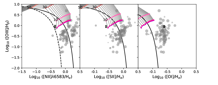
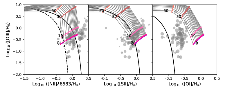
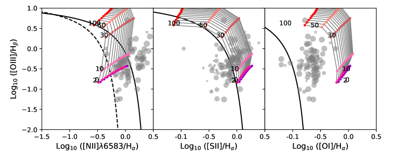
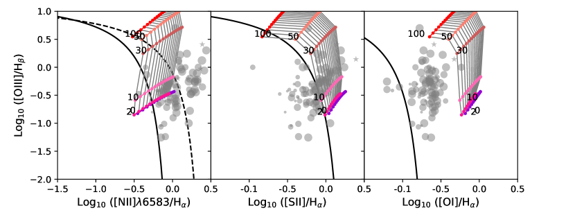
Figure 16: BPT diagrams. Comparison of the observed line ratios with the model predictions. The gray dots (filament values) and the stars (nucleus values) represent the data from Mcdonald et al. (2012). The size of the dots decreases with the increase of the distance from the nuclei of the corresponding object. The solid black line is the upper limit for HII  regions by Kewley et al. (2001) and the dashed black line is the lower limit for AGN by Kauffmann et al. (2003). The predicted cumulative line ratios from the models are overlaid. The gray lines correspond to a single value of metallicity and different values of turbulence (the velocity value is written on the left and reproduced with different colours); from left to right the velocity is constant and the metallicity increases (from 0.3 to 1 Z_⊙). The G_X  is fixed to 100.Left column: cumulative emission of [O iii]$\lambda$ 5007 $\AA$/H${\beta}$ vs. [N ii]$\lambda$ 6583 Å/H${\alpha}$; central column: [O iii]$\lambda$ 5007 $\AA$/H${\beta}$ vs. [S ii]/H${\alpha}$; right column: [O iii]$\lambda$ 5007 $\AA$/H${\beta}$ vs. [O i]/H${\alpha}$. Top row: cumulative emission at A_V = 0.001 mag; second row: cumulative emission at A_V = 0.1 mag; third row: cumulative emission at A_V = 1 mag; Bottom row: cumulative emission at A_V = 5 mag.

The combination of the line ratios [O iii]$\lambda$ 5007 $\AA$/H${\beta}$, [N ii]$\lambda$ 6583 Å/H${\alpha}$  ([S ii]$\lambda$ 6716 $\AA$+[S ii]$\lambda$ 6731 $\AA$)/H${\alpha}$  and [O i]$\lambda$ 6300 $\AA$/H${\alpha}$  are commonly used in the so-called BPT diagrams to identify the excitation mechanism of the optical line-emitting gas. Mcdonald et al. (2012) used this technique to investigate the contributors to the ionization of the filaments in nine cool-core galaxy clusters. Overlapping on the BPT diagrams grid of models from previous studies to the observed values, the authors eliminated most of the heating mechanisms suggested. We compare our grid of models with the observed values of their BCG sample in Fig. 5. To make easier the reading of these plots, we show in the Appendix E, as examples, the BPT diagrams varying Z and G_X  for a fixed turbulence of 10 km s^-1 (Figure 15), and those varying only the turbulence and the metallicity for single values of G_X= 100 (Figure 16). These figures show the line ratios predicted at different A_V: 0.001 mag (top row), 0.1 mag (second row), 1 mag (third row) and 5 mag (bottom row).

In Fig. 5 we can immediately see that, in general, our grid of models can reproduce the observables except the [O i]$\lambda$ 6300 $\AA$/H${\alpha}$ ratio. The observed values in the [N ii]-diagram are well reproduced at all of the explored A_V. Note that varying A_V  the best model that reproduces the specific observed ratio changes. Also the predicted ([S ii]$\lambda$ 6716 $\AA$+[S ii]$\lambda$ 6731 $\AA$)/H${\alpha}$  are in agreement with the data, even if increasing A_V  increases the predicted ([S ii]$\lambda$ 6716 $\AA$+[S ii]$\lambda$ 6731 $\AA$)/H${\alpha}$  ratio. The predicted [O i]$\lambda$ 6300 $\AA$/H${\alpha}$, instead, are in agreement with the observables only for very low A_V  (A_V = 10^-3 mag). Table 2 summarizes which is, among all of the models, the restricted parameter space that can reproduce the optical observations. The range of G_X  values that can reproduce most of the observables, for any metallicity, moves to lower values with the increasing of the turbulence and higher values with the increasing of A_V. The different position of the models on the BPT-diagrams highlights the impact of G_X, turbulence and A_V  on the physical properties (i.e., temperature, electron fraction, density) of the cloud and thus, affect the ratio of the optical line ratios.

The optical line ratios of the BPT-diagrams trace different sections of the cloud. As described in the previous section, [O iii]$\lambda$ 5007 $\AA$  arises from the outskirt of the environment compared to [N ii]$\lambda$ 6583 Å, and [S ii] lines, while [O i]$\lambda$ 6300 $\AA$, which traces warm dense gas, comes from the ionized front. Thus, varying A_V  affects the line ratios for a given combination of G_X  and turbulence. For those models with low excitation sources (low G_X  and turbulence) the cloud does not have an ionized phase, thus there is no impact of the variation of A_V  on the line ratios. The increase of G_X  and/or the turbulence moves the ionized front deeper into the cloud. Thus, for those models with excitation sources strong enough to ionized the gas, varying A_V  changes the relative phase distribution of the clouds, and consequently the predicted optical line ratios vary. In particular the increasing of the over-estimation of [O i]$\lambda$ 6300 $\AA$/H${\alpha}$ with A_V, suggests that the observed optical emission arise from a cloud with low A_V, in other words, a large fraction of the gas in the filaments can be reproduce by a matter bounded cloud.

We note that the observed [O iii]$\lambda$ 5007 $\AA$/H${\beta}$  ratio given by Mcdonald et al. (2012) can be very small (0.1-0.03). This was already discussed in Hatch et al. (2006) who noticed the unexpected complete lack of [O iii]$\lambda$ 5007 $\AA$  in most of the regions inside the filaments around NGC 1275. The observed optical line ratios may have several excitation mechanisms, such as star-formation and particle excitation, which may be varying the [O iii]$\lambda$ 5007 $\AA$/H${\beta}$  line ratio. The small values in Mcdonald et al. (2012) correspond to regions where there is not evidence of star-formation. Powering the optical nebula without strong [O iii]$\lambda$ 5007 $\AA$  line can be explained if cosmic ray heating/ionization is invoked as described by Ferland et al. (2009). Another solution is the strategy adopted in this work, i.e. use an EUV continuum that can reproduce the observed optical line ratios (see Sec. 2.1.1). We leave for a future work the detailed comparison of the current model predictions with the observed emission lines in the filaments of NGC 1275.

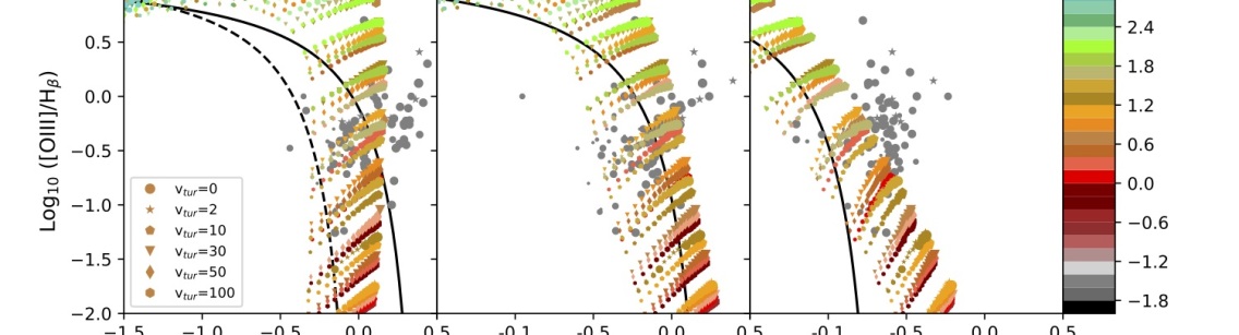
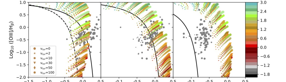
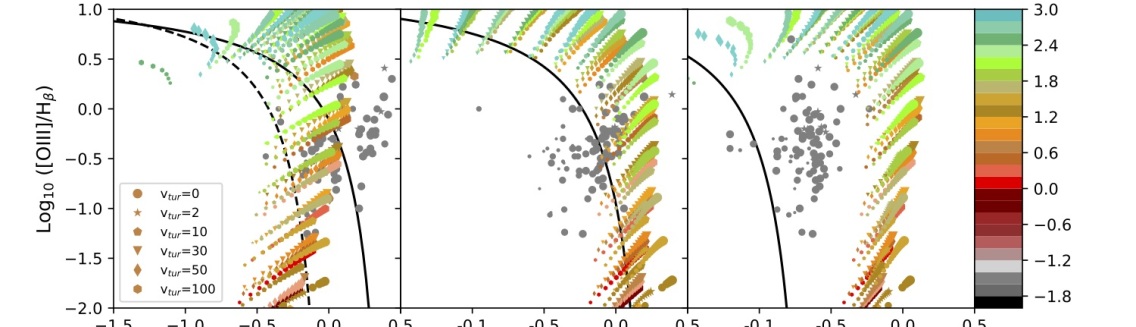
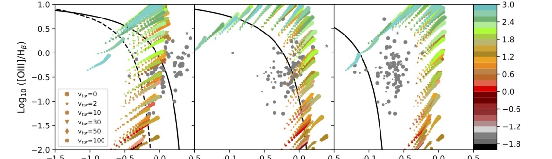
Figure 5: BPT diagrams. The gray dots (filament values) and the stars (nucleus values) represent the data from Mcdonald et al. (2012). The size of the dots decreases with the increasing of the distance from the nuclei of the corresponding object. The solid black line is the upper limit for HII  regions by Kewley et al. (2001) and the dashed black line is the lower limit for AGN by Kauffmann et al. (2003). The predicted cumulative line ratios from the models are overlapped. The color bar correspond to the different values of G_X  (the logarithm of the value is written on the bar); each symbol correspond to one turbulence value and the size of the symbols increase with the metallicity (from 0.3 to 1 Z_⊙). Top row: cumulative emission at A_V = 0.001 mag; second row: cumulative emission at A_V = 0.1 mag; third row: cumulative emission at A_V = 1 mag; Bottom row: cumulative emission at A_V = 5 mag. Left column: [O iii]$\lambda$ 5007 $\AA$/H${\beta}$ vs. [N ii]$\lambda$ 6583 Å/H${\alpha}$; central column: [O iii]$\lambda$ 5007 $\AA$/H${\beta}$ vs. [S ii]/H${\alpha}$; right column: [O iii]$\lambda$ 5007 $\AA$/H${\beta}$ vs. [O i]/H${\alpha}$.

Table 2: Restricted ranges of free parameters are given for 4 values of A_V = 0.001, 0.1, 1 and 5 mag.

Turbulence	AV	GX	Z	AV	GX	Z	AV	GX	Z	AV	log10GX	Z
$[$km s-1]	[mag]		Z⊙	[mag]		Z⊙	[mag]		Z⊙	[mag]		Z⊙
0	0.001	101.2 - 102	all	0.1	101.6 - 102.6	all	1	101.6 - 103	all	5	101.6 - 103	all
2		101.2 - 102	all		101.6 - 102.6	all		101.6 - 103	all		101.6 - 103	all
10		101 - 102	all		101.4 - 102.4	all		101.6 - 102.8	all		101.6 - 103	all
30		100.6 - 101.4	all		10 - 100	all		10 - 102.2	all		10 - 102.4	all
50		100.2 - 101	all		100.6 - 101.6	all		100.6 - 101.8	all		100.6 - 102.2	all
100		10-0.2 - 100.6	all		1 - 101.2	all		100.2 - 101.4	all		1 - 101.6	all

3.2 Infrared tracers

Unlike the optical lines, infrared observations are not affected significantly by extinction and they cover a wide range of ionization potentials and critical densities. Moreover, line ratios of infrared lines are almost independent from the temperature.

3.2.1 [Ne ii]$\lambda$ 12.8 $\mu$m/[Ne iii]$\lambda$ 15.5 $\mu$m

The line ratio [Ne ii]$\lambda$ 12.8 $\mu$m/[Ne iii]$\lambda$ 15.5 $\mu$m, is a perfect tracer of the intensity of the radiation source, since the two lines are emitted by the same element but with different ionization stages. The [Ne iii]$\lambda$ 15.5 $\mu$m has higher ionization potential than [Ne ii]$\lambda$ 12.8 $\mu$m, 41 eV and 21.6 eV, respectively, and they have similar critical density, 3$\times$10⁵ cm^-3 for [Ne iii]$\lambda$ 15.5 $\mu$m and 7$\times$10⁵ cm^-3 for [Ne ii]$\lambda$ 12.8 $\mu$m. Both lines are found exclusively in HII  regions, with [Ne iii]$\lambda$ 15.5 $\mu$m  arising from the layer closer to the radiative source compared to [Ne ii]$\lambda$ 12.8 $\mu$m. These two lines have been detected for several BCGs with the IRS instrument onboard of Spitzer. We collected the observed ratio [Ne ii]/[Ne iii] for a total of 10 BCGs (values from Donahue et al. 2011, Egami et al. 2006, and Johnstone et al. 2007) and compare them with the predicted line ratio from our grid of models. The comparison is shown in Figure 6, top row. The observed ratio of the full sample covers the range between 1.10 and 5.25, and it is represented by the blue background. We do not present the theoretical line ratio for all of the models, but only for few representative cases, with the aim of understanding how the ratio changes as a function of the free parameters: G_X, turbulence, metallicity and A_V. On the left panel we fix v_tur and Z, and we vary only G_X. For low G_X, the model can not reproduce the observables. Increasing the intensity of the radiation field the model produces more energetic photons, boosts [Ne iii]$\lambda$ 15.5 $\mu$m  and the ratio decreases, with lower values at low A_V. After the ionization front, the ratio becomes constant. Similar behavior is shown varying only the turbulence (central panel). We see that the combination of G_X= 10 and v_tur= 0-2 km s^-1 can reproduce the observed range at every A_V. The increasing of v_tur boosts [Ne iii]$\lambda$ 15.5 $\mu$m and moves the predicted values that can reproduce the observations inside the cloud. The consequence of the variation of metallicity on the [Ne ii]/[Ne iii] ratio is almost negligible and all of the model with v_tur = 10 km s^-1 and G_X=10 can reproduce the observed ratio (right panel). The restricted range of the parameter space that can reproduce the observations taking into account all of the models is presented in Table 3. The models with G_X between 1 to 10³ can reproduce the line ratio for an extended range of A_V. The smallest value of A_V  which match observed [Ne ii]/[Ne iii] ratio varies with the combination of G_X  and v_tur. The variation of the metallicity affects slightly the behavior of the predicted line ratio. The impact of the metallicity on the range of A_V  is indicated in Table 3 with different letters.

3.2.2 [O i]$\lambda$ 63.2 $\mu$m/[C ii]$\lambda$ 157.7 $\mu$m

The far-infrared line ratio [O i]$\lambda$ 63.2 $\mu$m/[C ii]$\lambda$ 157.7 $\mu$m  observed by Herschel is a good tracer of the electron density if the lines are optically thin, since the critical densities of these two lines are different. The critical density for [O i]$\lambda$ 63.2 $\mu$m is $\sim$5$\times$10⁵ cm^-3, and for [C ii]$\lambda$ 157.7 $\mu$m is $\sim$3$\times$10³ cm^-3, much higher. The range of observed [O i]$\lambda$ 63.2 $\mu$m/[C ii]$\lambda$ 157.7 $\mu$m line ratios (0.22 - 1.64) is shown, in the central row of Figure 6, as the green background (values from Edge et al. 2010, Mittal et al. 2011, Mittal et al. 2012, and Werner et al. 2014). Our models match those observations for a large range of free parameters, as summarized in Table 3. Since Carbon and Oxygen abundances are scaled by the same factor, the metallicity has very little impact on this line ratio, while the variation of G_X  and turbulence has a clear consequences on the profile of the [O i]$\lambda$ 63.2 $\mu$m/[C ii]$\lambda$ 157.7 $\mu$m line ratios. For a fixed value of G_X, the range of A_V that fit the data increases with the increasing of the turbulence. The same behaviour can be observed for models with a fixed value of v_tur and different G_X, i.e. increasing G_X  moves the minimum value of the range of A_V  that fit the data to higher A_V.

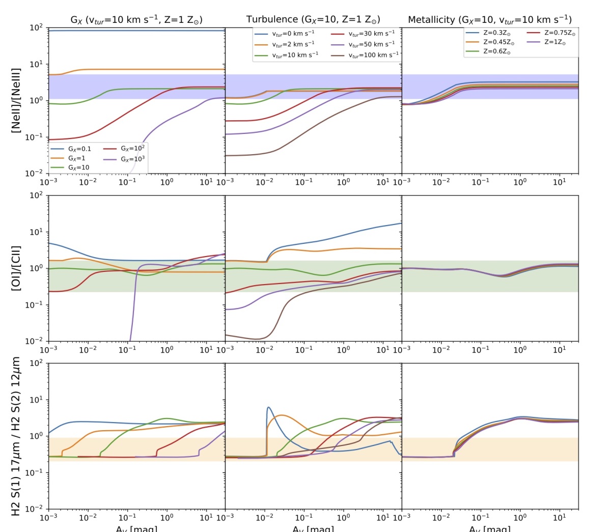
Figure 6: Comparison of observed and predicted cumulative line ratios: [NeII]/[NeIII] (top), [O i]$\lambda$ 63.2 $\mu$m/[C ii]$\lambda$ 157.7 $\mu$m (middle) and H₂ S(1) 17.0 $\mu$m/H₂ S(2) 12.3 $\mu$m (bottom), as a function of A_V. The blue background highlights the observed line ratio of [NeII]/[NeIII], range of values between 1.10 and 5.25 (data from Donahue et al. 2011, Egami et al. 2006, and Johnstone et al. 2007). The observed line ratio [O i]$\lambda$ 63.2 $\mu$m/[C ii]$\lambda$ 157.7 $\mu$m  range, between 0.22 to 1.64 (values from Edge et al. 2010, Mittal et al. 2011, Mittal et al. 2012, and Werner et al. 2014), is shown in green, and the yellow background highlights the observed ratio of the two pure rotational H₂ lines, between 0.2 and 0.9 (values from Donahue et al. 2011, Egami et al. 2006, and Johnstone et al. 2007). The column on the left shows the predicted ratios for models with v_tur = 10 km s^-1 and solar metallicity, the central column the ratios for models with G_X=10 and solar metallicity and the column on the right the ratios for models with v_tur = 10 km s^-1 and G_X=10.

Table 3: Restricted parameter space of the free parameters that reproduce the infrared observations.

Line or ratio	Turbulence	GX	AV	Z	Turbulence	GX	AV	Z
	$[$km s-1]		[mag]		$[$km s-1]		[mag]
$[$NeII]/[NeIII]	0	10	all	A	30	1	all	A
		100	$\geq$0.1	B		10	$\geq$0.1	B
		103	$\geq$7	B		100	$\geq$0.3	B
$[$OI]/[CII]		10	$\leq$0.01	A		0.1, 1, 10	all	A
						100	$\geq$0.03	B
						103	$\geq$0.4	B
H2 0-0 S(1)/		0.1	$\leq$0.02	C		0.1	$\leq$0.003	F
H2 0-0 S(2)		1	$\geq$0.08	A		1	$\leq$0.03	F
		10	$\leq$0.01 and $\geq$0.03	D		10	$\leq$0.3	F
		100	$\leq$0.2 and $\geq$1	C		100	$\leq$7	F
		103	$\leq$3 and $\geq$20	A		103	$\geq$0.3	F
$[$NeII]/[NeIII]	2	10	all	A	50	0.1	all	A
		100	$\geq$0.2	B		1	$\geq$0.02	B
		103	$\geq$10	B		10	$\geq$0.5	A
$[$OI]/[CII]		10	$\leq$0.01	A		0.1, 1	all	B
		100	$\leq$ 0.2	E		10	$\geq$0.02	B
		103	between 0.07 and 2	B		100	$\geq$0.01	B
						103	$\geq$1	B
H2 0-0 S(1)/		10	$\leq$0.01	A		0.1	$\leq$0.003	F
H2 0-0 S(2)		100	$\leq$0.2	E		1	$\leq$0.04	F
		103	$\leq$4	A		10	$\leq$1	F
						100	between 0.07 and 10	F
						103	$\geq$1	E
$[$NeII]/[NeIII]	10	1	$\leq$0.003	F	100	0.1	all	A
		10	$\geq$0.01	B		1	$\geq$0.1	B
		100	$\geq$0.3	B		10	$\geq$3	B
		103	$\geq$10	B
$[$OI]/[CII]		0.1	$\geq$0.02	B		0.1	$\leq$0.01 and $\geq$0.7	A
		1	all	A		1	$\geq$0.02	B
		10	all	A		10	$\geq$0.1	B
		100	$\leq$3	A		100	$\geq$0.3	B
		103	between 0.01 and 10	B		100	$\geq$3	B
H2 0-0 S(1)/		1	$\leq$0.008	F		0.1	$\leq$0.01	F
H2 0-0 S(2)		10	$\leq$0.05	F		1	$\leq$0.2	F
		100	$\leq$3	F		10	between 0.02 and 3	F
		103	$\leq$20	F		100	$\geq$0.3	F
						103	$\geq$3	B

Notes. A = There is not difference in the range due to the variation of Z.
B = The minimum value of A_V  decreases with the decreasing of Z.
C = The minimum value of A_V  increases with the decreasing of Z.
D = The range of A_V  that can reproduce the observed values moves to lower A_V  for lower Z.
E = The maximum value of A_V  increases with the decreasing of Z.
F = The maximum value of A_V  decreases with the decreasing of Z.

3.2.3 Pure rotational H₂ lines

In the infrared we can also detect the line emission of the warm molecular gas ($\geq$100 K) emitted by the rotational and vibrational H₂ transitions. In the bottom row of Figure 6, we compare the observed H₂ pure rotational line ratio S(1)17$\mu$m/S(2)12$\mu$m (values from Donahue et al. 2011, Egami et al. 2006, and Johnstone et al. 2007) to our model predictions. The observed line ratio is between 0.2 and 0.9, represented by the orange background, and the predicted line ratios from representative models are shown as a function of A_V. At a moderate constant turbulent heating rate (v_tur = 10 km, left panel), because the S(1) line has a lower excitation temperature than the S(2) line, all models show an increase of the H₂ S(1)/S(2) line ratio with A_V, except for very low G_X  where it is roughly constant (in that case the cloud temperature is almost constant at A_V¿ 0.01). We note that the models match the observed range of ratios where the medium is mostly atomic. For a fixed G_X=10 and solar metallicity (middle panel), the observed ratio can be reproduced by all of the turbulence values, but for a different range of A_V. Finally, the metallicity affects only slightly the behavior of the predicted line ratio (right panel). The summary of the combination of free parameter values that can reproduce the observed ratio H₂ S(1) 17.0 $\mu$m/S(2) 12.3 $\mu$m is provided in Table 3.

3.2.4 Ro-vibrational H₂ lines

Also the ro-vibrational H₂ lines that emits $\sim$2 $\mu$m have been observed in several BCGs, and presented by Edge et al. (2002). In Figure 7 we compere the observed values of H₂ 1-0 S(3), H₂ 1-0 S(2), H₂ 1-0 S(1) and H₂ 1-0 S(0), normalized by Pa_α, to our predicted H₂/Pa_α, ratios. In our models, these line emission are excited by the collision with the secondary electrons produced by the interaction of the X-ray radiation field with the medium. For most of our models, this excitation mechanism is enough to produce the H₂ emission inside the cloud and we do not need to add cosmic rays. Increasing the X-ray radiation field intensity (left column) the peak of the emission moves to higher A_V. Consequently the cumulative intensity of the H₂ lines reaches higher values deeper into the cloud. However, the increasing of G_X  decreases the density of the cloud at low A_V, thus the cumulative emission profiles of these lines become steeper. The variation of the turbulence, instead, do not changes the values of the secondary electron rate (central column), but it affects the structure of the cloud (see sec. 2.2). The combination of these two factors pushes the intensity of the ro-vibrational lines down for higher turbulence. Finally, with the increasing of the metallicity (right column) the line emission decrease. All of the models that we show in Fig. 7 can reproduce the normalized ro-vibrational line emission, even if at different A_V.

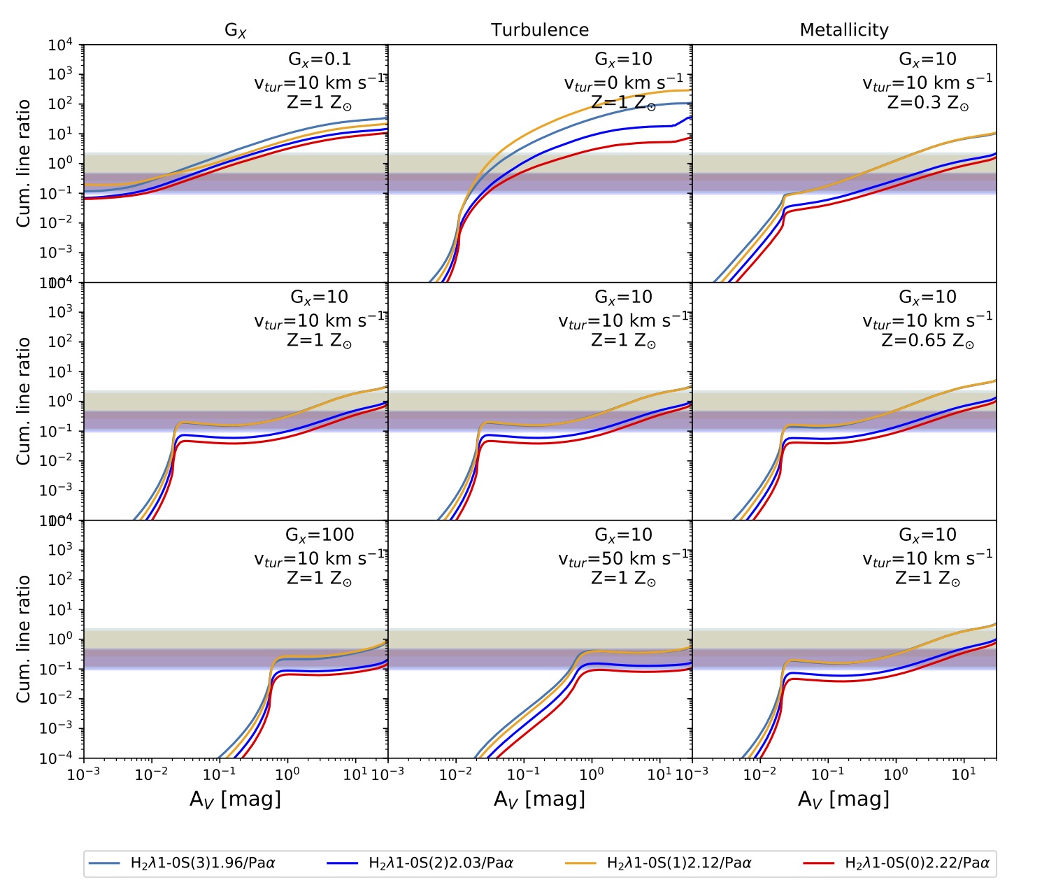
Figure 7: Comparison of observed and predicted ro-vibrational H₂ lines, normalized by Pa$\alpha$, as a function of A_V  for the models described in Sect. 2.2. The different background highlights the observed ratios, between 0.1 and 2.3 (values from Edge et al. 2002). For each ratio, the color of the background is the same of that of the theoretical cumulative ratio. The column on the left shows the predicted cumulative emission for models with turbulence of 10 km s^-1, solar metallicity and various values of G_X: 0.1 (top), 10 (middle) and 100 (bottom); the central column shows the predicted cumulative emission for models with G_X=10, solar metallicity and various values of turbulence: 0 (top), 10 (medium) and 50 (bottom) km s^-1; the column on the right shows the predicted cumulative emission for models with turbulence 10 km s^-1, G_X=10 and various values of metallicity: 0.3 (top), 0.65 (middle) and 1 (bottom) Z_⊙.

3.3 Sub-millimeter lines

Finally, we compare the predicted CO(1-0), (2-1), (3-2) transitions, which trace the cold ($\sim$10K) molecular gas, to the observations presented in Salomé et al. (2008). Figure 8 shows the observed range of CO (1-0) and CO (2-1) with a green and a blue background, respectively, and the predicted values of the three transitions for models with fixed turbulence and metallicity but different values of G_X(left panel), and for models with fixed G_X  and metallicity but varying the turbulence (right panel). Since the cold molecular gas traced by the CO transitions is expected to arise from the deepest region of the cloud, we compared the observations only with the predicted cumulative emission at A_V=30 mag. For a fixed v_tur=10 km s^-1  and Z=Z_⊙, all the models with G_X $\geq$10 can reproduce the observed CO(1-0) and all the models with G_X $\geq$1.6 can reproduce the observed emission CO(2-1). While, fixing Z=Z_⊙ and G_X=10, only the model with v_tur = 10 and 30 km s^-1  can reproduce both transitions. These comparisons restrict drastically the ‘good’ parameter space, in particular the turbulence. We would like to remind that these results are based on a single model component and a more complex multi-component model could bring different results. An additional limitation in these models is that the turbulence is treated as a constant heating rate everywhere in the cloud, which is unrealistic.

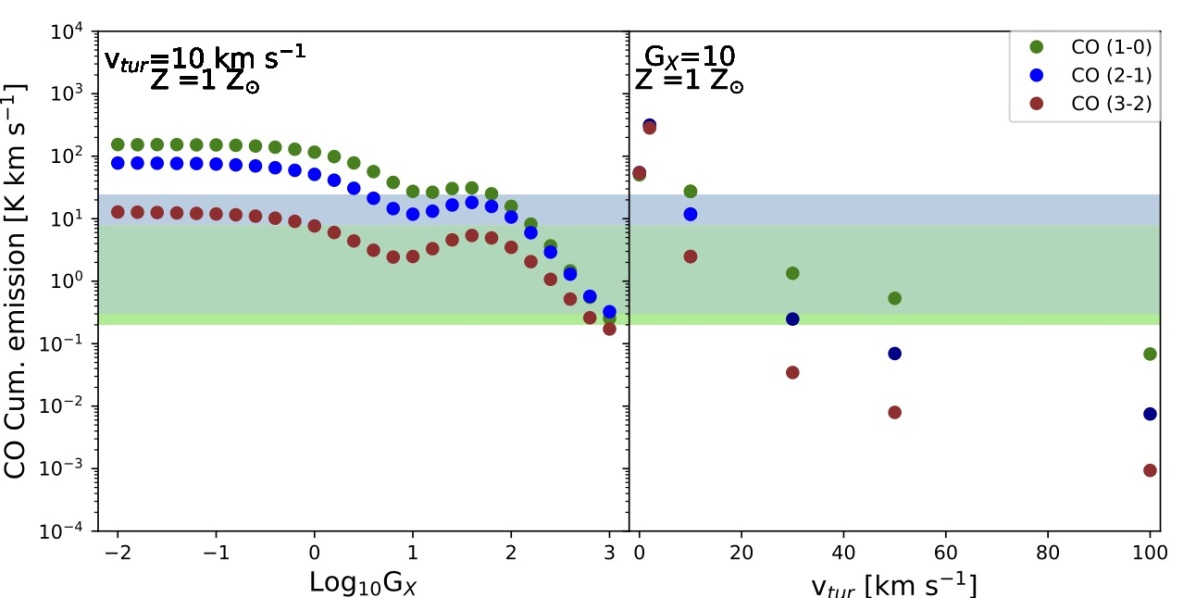
Figure 8: Comparison of observed (green and blue background) and predicted cumulative CO emission: 1-0, 2-1 and 3-2. The predicted values are for A_V=30 mag (end of the cloud). The panel on the left shows the predicted values as a function of G_X, for models with turbulence of 10 km s^-1  and solar metallicity. The panel on the right shows the predicted values as a function of turbulence, for models with G_X=10 of and solar metallicity.

4 Origin of the soft X-ray/EUV emission

The actual model assumes that the soft X-ray and the EUV photons that power the nebula are produced by the cooling of the hot ICM in the filaments. In this section, we investigate whether the input X-ray intensity of our models can power the total line intensities, and we compare with observational estimates from the Perseus cluster.

To give orders of magnitude, a G_X=10 corresponds to an input X-ray surface brightness in the range 0.6-3.4 keV of $\sim$4 $\times$ 10^-14 erg cm^-2 s^-1 arcsec^-2. For a typical filament in Perseus of 27”$\times$1” at the distance of 80 Mpc, this means a luminosity of $\sim$1$\times$10⁴² erg s^-1. Sanders & Fabian 2007 analyzed the X-ray emission in a region of 27.3 $\times$ 1 arcsec². They computed that the difference in temperature of the cooling X-ray emitting gas from the surrounding gas was $\sim$2.7 keV. This imply a released energy of $\sim$2.5$\times$10⁵⁴ erg if the X-ray emitting filament was to cool out of the surrounding ICM. Assuming a timescale for this process of $\sim$10⁵ yr, they conclude that the gas cooling provides enough energy to power about 10⁴² erg/s.

The authors also discuss the fact that the X-ray surface brightness in 0.5-2 keV is almost similar to the H${\alpha}$+[N ii]$\lambda$ 6583 Å surface brightness given by Conselice et al. (2001) (Fig.18 of Sanders & Fabian 2007). In order to account for the total reprocessed emission in all the different lines, they estimate that the input power must be a factor of 20 larger than the one required for the H${\alpha}$ only. This leads to a required input power of $\sim$10⁴² erg/s for a typical filament in the Perseus cluster. The present models show that the predicted surface brightness in the range 0.6-2 keV is similar to the predicted H${\alpha}$+[N ii]$\lambda$ 6548, 6583 $\AA$  surface brightness for A_V $>$20, which corresponds to hydrogen column density $\sim$10²² cm^-2. A cloud with large optical depths is needed to reprocess the X-rays and excite the infrared H₂ lines (Figure 7). As an example, Figure 9 shows the behavior of the two emissions for the model with G_X=10, v_tur=10 km s^-1 and Z=Z_⊙. The predicted surface brightness of the reprocessed soft X-ray from the model is comparable with the observed value, 4.3$\times$10^-16 erg cm^-2 s^-1arcsec^-2, within a factor of three for A_V$\geq$18 mag. The H${\alpha}$+[N ii]$\lambda$ 6548, 6583 $\AA$  surface brightness, instead, is under-predicted by a factor of $\sim$4. It is important to remind that large uncertainties are related to the observations, such as the extinction correction for both Galactic and internal reddening (e.g. Johnstone et al. 2007). Nevertheless, this discrepancy between the observed and the predicted H${\alpha}$+[N ii]$\lambda$ 6548, 6583 $\AA$  suggests caveats in our models, which could be related to the a priori assumptions.

Table 6 presents the list of the twenty brightest predicted line emission at different A_V  for the seven models described in this paper, ordered from the brightest to the fainter. The total energy released obviously depends on the parameters of a given model but is enough to power all the different lines.

There is a range of specific models for which (i) the input X-ray energy is similar to the value estimated in Sanders & Fabian (2007) if coming from self-irradiation by the cooling gas, (ii) this energy is enough to power the total line emission, and produce outwards X-ray surface brightness comparable to the observed value for A_V $\geq$5 mag.

Finally, the actual models produce very faint or even no O vi $\lambda$1032,1038$\AA$ doublet. For example, for G_X=100 the surface brightness of these lines is of the order of 10^-24 erg cm^-2 s^-1 arcsec^-2, while that of H${\alpha}$ is $\sim$10^-15 erg cm^-2 s^-1 arcsec^-2. This is in agreement with the no-detection of these lines shown by Lecavelier des Etangs et al. (2004). However, observations reveal a tension in this regard, since other works have detected O vi doublet at the center of some cool-core clusters (e.g. Bregman et al. 2006). The O vi line emission can be enhanced in radiative shocks and mixing layers (e.g. McQuinn & Werk 2018; Ji et al. 2019), which are not considered in our models.

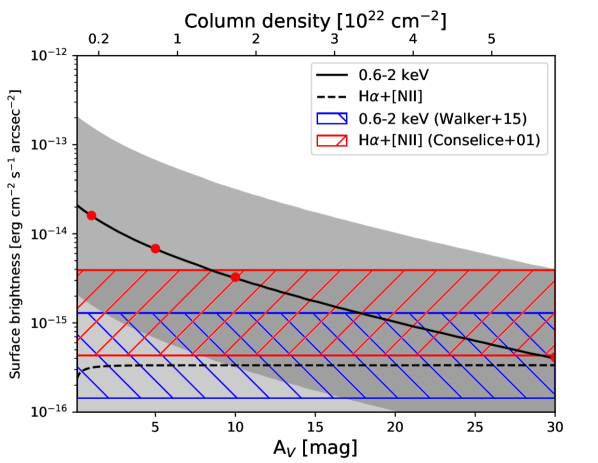
Figure 9: Predicted cumulative surface brightness of H${\alpha}$+[N ii]$\lambda$ 6548, 6583 $\AA$  (dashed line) and predicted ionizing continuum 0.6-2 keV X-ray band (solid line) as a function of A_V  for a model with G_X=10, v_tur=10 km s^-1  and Z=Z_⊙. The dark grey and soft grey background show the range of predicted ionizing continuum 0.6-2 keV X-ray and cumulative surface brightness of H${\alpha}$+[N ii]$\lambda$ 6583 Å, respectively, for models with G_X  in the range 1 - 100. The red dots show the predicted transmitted continuum 0.6-2 keV X-ray band estimated at A_V = 1, 5, 10, 30 mag. The area covered by red (blue) diagonal lines represent a factor of three of the observed surface brightness of H${\alpha}$+[N ii]$\lambda$ 6548, 6583 $\AA$  from Conselice et al. (2001) for the region 15 of the paper, 1.3$\times$10^-15 erg cm^-2 s^-1arcsec^-2 (of 0.6-2 keV X-ray band from Walker et al. (2015), 4.3$\times$10^-16 erg cm^-2 s^-1arcsec^-2).

5 Conclusions

This article presents the modelling of the physical, chemical structure and line emission of filaments surrounding BCGs. We use the Cloudy  code to revisit a self-irradiated model where the source of photoionization and heating of the filaments is the cooling radiation from the hot ICM plasma (the so-called cooling flow). The energy source is assumed to be the radiation from the gas cooling out of the hot plasma. We explore the effect of the penetration of the photons inside the clouds by varying A_V. As a result, the grid of models predicts the emission lines arising from the ionized, neutral and molecular regions. We also explore turning on additional (turbulent) heating and we discuss the impact of such another source of heating that acts as an extra-pressure.

The structure of the clouds changes as the free parameter change. Increasing the intensity of the radiation field, the temperature and the ionization fraction of the gas also increase, while the density decreases (the models are isobaric). For low X-ray intensity the edge of the cloud is atomic and becomes molecular inside. Increasing the intensity, the ionization and molecular fronts move to higher A_V. Increasing the turbulence has similar effects, while increasing the metallicity moves to lower A_V the transition between the ionized and the atomic region. Changing the metallicity has less dramatic consequences on the model predictions.

We note that the important parameters are (i) the slope of the input radiation field: the power law used in Cloudy to model X-ray cooling flows that produces the soft X-ray and EUV photons that play a major role in the gas ionization; (ii) the strength of the input X-ray radiation field; (iii) the Av; and (iv) the level of turbulence, which provides extra-heating through dissipation of energy. There is an unavoidable degeneracy in the impact of these parameters, but it is clear that without any X-ray source it is not possible to reproduce the observations.

We have compared our grid of models to the rich range of observations now achieved in cool core cluster. Filaments in BCGs have been mapped from the soft X-ray to the millimeter and many lines in the optical and the infrared have been detected. We have used such data to restrict the plausible range of parameter. The different combination of the free parameters presented in this paper can reproduce the multi-wavelength observables without requiring an excess of X-ray luminosity. The emitted intensity in the X-ray from Sanders et al. (2005) and Walker et al. (2015) is in agreement with the estimated reprocessed emitted intensity in the 2-10 keV band as well as 0.6-2 keV band of the models with G_X$\sim$10 and the X-ray input energy is enough to power the line emission.

Within a reduced range of parameter, some models can simultaneously reproduce most of the ionized and molecular lines. The combination of G_X  between 1 to 10³, any metallicity and turbulence that varies according to the selected G_X, for Av between 0.1 and 10 mag reproduces the typical BCG LINER-like low-ionization line ratio observed in BPT-diagrams, including [O iii], [O i] being more difficult to reproduce if not at very low Av (less then 0.1 mag). This restricted range of parameter space reproduces the infrared ratios as well. We note that the MIR and FIR lines arising from the atomic and molecular gas phases are very dependent on the A_V. Finally, only the models with v_tur=10 or 30 km s^-1  and G_X$\geq$ 10 can reproduce the observed CO transitions.

It is clear that the mechanisms powering the nebula are more complex than these simple single component plane-parallel models of a constant pressure self-irradiated clouds. A better representation of the filaments may come from a combination of such models as expected for a population of clouds with a range of A_V illuminated by different G_X and extra-heating. We are aware that a constant pressure model is a simplification and we also expect a contribution of energetic particles and of star formation in some regions but this was out of the scope of the actual study. In future, new constraints from high resolution multi-wavelength line emission as well as molecular absorption line, from Multi Unit Spectroscopic Explorer (MUSE) and Atacama Large Millimeter/submillimeter Array (ALMA), for several BCGs will help to developed a more complex modeling.

In a future paper we will use the restricted grid of model identified in this study to model the multi-wavelengths observations of the filamentary regions surrounding NGC 1275.

Appendix A Chemical ISM composition

The gas and dust elemental abundances used in our models are those given by Cloudy  for the interstellar medium case. We report in Table 4 the values for the gas-phase and in Table 5 the values for the dust conposition.

Table 4: Gas-phase abundances used in our models.

Element	Abundances	Element	Abundances
He/H	9.50$\times 10^{-02}$	Li/H	5.40$\times 10^{-11}$
Be/H	1.00$\times 10^{-20}$	B/H	8.90$\times 10^{-11}$
C/H	3.00$\times 10^{-04}$	N/H	7.00$\times 10^{-05}$
O/H	4.00$\times 10^{-04}$	F/H	1.00$\times 10^{-20}$
Ne/H	6.00$\times 10^{-05}$	Na/H	3.00$\times 10^{-07}$
Mg/H	3.00$\times 10^{-06}$	Al/H	2.00$\times 10^{-07}$
Si/H	4.00$\times 10^{-06}$	P/H	1.60$\times 10^{-07}$
S/H	1.00$\times 10^{-05}$	Cl/H	1.00$\times 10^{-07}$
Ar/H	3.00$\times 10^{-06}$	K/H	1.10$\times 10^{-08}$
Ca/H	2.00$\times 10^{-08}$	Sc/H	1.00$\times 10^{-20}$
Ti/H	5.80$\times 10^{-10}$	V/H	1.00$\times 10^{-10}$
Cr/H	1.00$\times 10^{-08}$	Mn/H	2.30$\times 10^{-08}$
Fe/H	3.00$\times 10^{-06}$	Co/H	1.00$\times 10^{-20}$
Ni/H	1.00$\times 10^{-07}$	Cu/H	1.50$\times 10^{-09}$
Zn/H	2.00$\times 10^{-08}$

Table 5: Grain abundances used in our models.

Element	Abundances	Element	Abundances
C/H	2.81$\times 10^{-04}$	O/H	1.31$\times 10^{-04}$
Mg/H	3.28$\times 10^{-05}$	Si/H	3.28$\times 10^{-05}$
Fe/H	3.28$\times 10^{-05}$

Appendix B Input parameters for the model with G_X=10, v_tur=10km s^-1  and Z =1 Z_⊙

table HM05 z = 0
table SED ”cool.sed”
intensity -1.8, range 14.71 to 147.06 Ryd
table sed ”test$\_$modif.sed”
f(nu) -16.8611 0.1755
cosmic ray background 0
turbulence 10 km/s
hden 2
constant pressure no continuum set 6.5
no grain molecules
database H2
abundances he = -1.022 li = -10.268 be = -20.000 b = -10.051 c = -3.523 n = -4.155
continue o = -3.398 f = -20.000 ne = -4.222 na = -6.523 mg = -5.523 al = -6.699
continue si=-5.398 p=-6.796 s=-5.000 cl=-7.000 ar=-5.523 k = -7.959
continue ca = -7.699 sc = -20.000 ti = -9.237 v = -10.000 cr = -8.000 mn = -7.638
continue fe = -5.523 co = -20.000 ni = -7.000 cu = -8.824 zn = -7.6990 no grains
grains ism
grains pah
metals and grains 1
set pah constant -4.6
set H2 Jura rate

Appendix C Comparison between our initial radiation field and the SED used by Ferland et al. 1994

Figure 10 shows the input SED used in Ferland et al. (1994), in green, and the input SED of one of our models, i.e.G_X=10, as an example, in black. The input SED used by Ferland et al. (1994) is too faint compared to the more recent surface brightness measurements by Walker et al. 2015 represented by the red star.

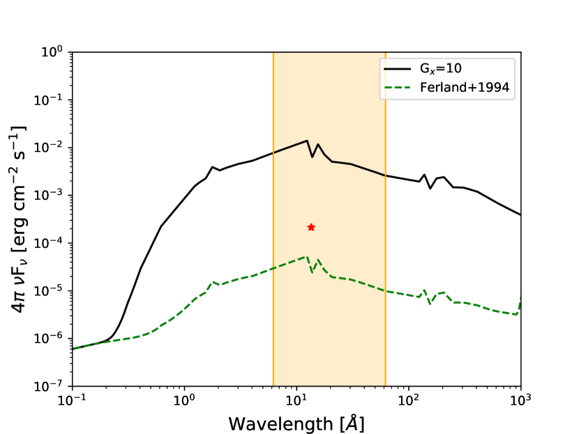
Figure 10: Comparison of the X-ray component of one of the input SED used in this study, i.e.G_X=10 (black curve), with that of the input SED used in Ferland et al. (1994) (green dashed curve). The red star represents the observed surface brightness measurements by Walker et al. 2015.

Appendix D Metallicity and turbulence effects in the structure of the cloud

Figures 12 and 12 show the consequences of different turbulent velocity on the structure of the cloud and Figures 13 and 14 the effects of varying the metallicity. The Figures are described in Sec. 2.2.

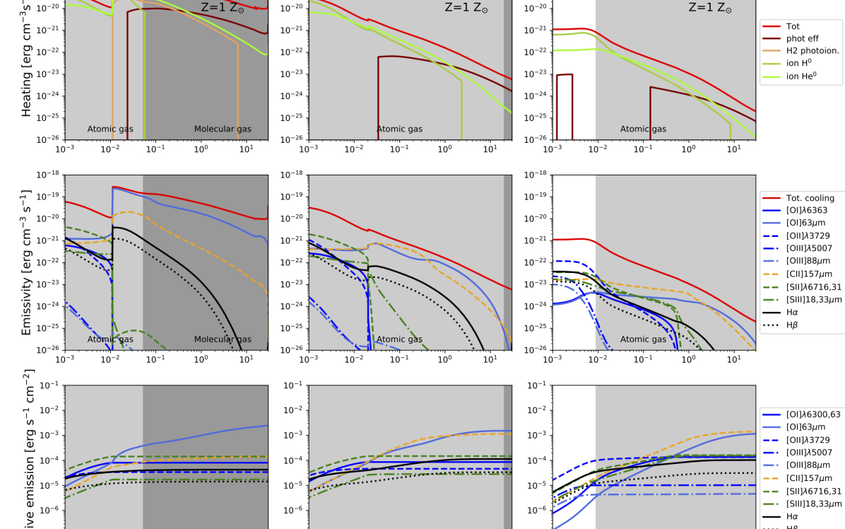
Figure 12: Same as Fig. 4, but this time G_Xis fixed at 10 and the turbulence varies: 0 km s^-1 (left column), 10 km s^-1 (central column) and 50 km s^-1 (right column).

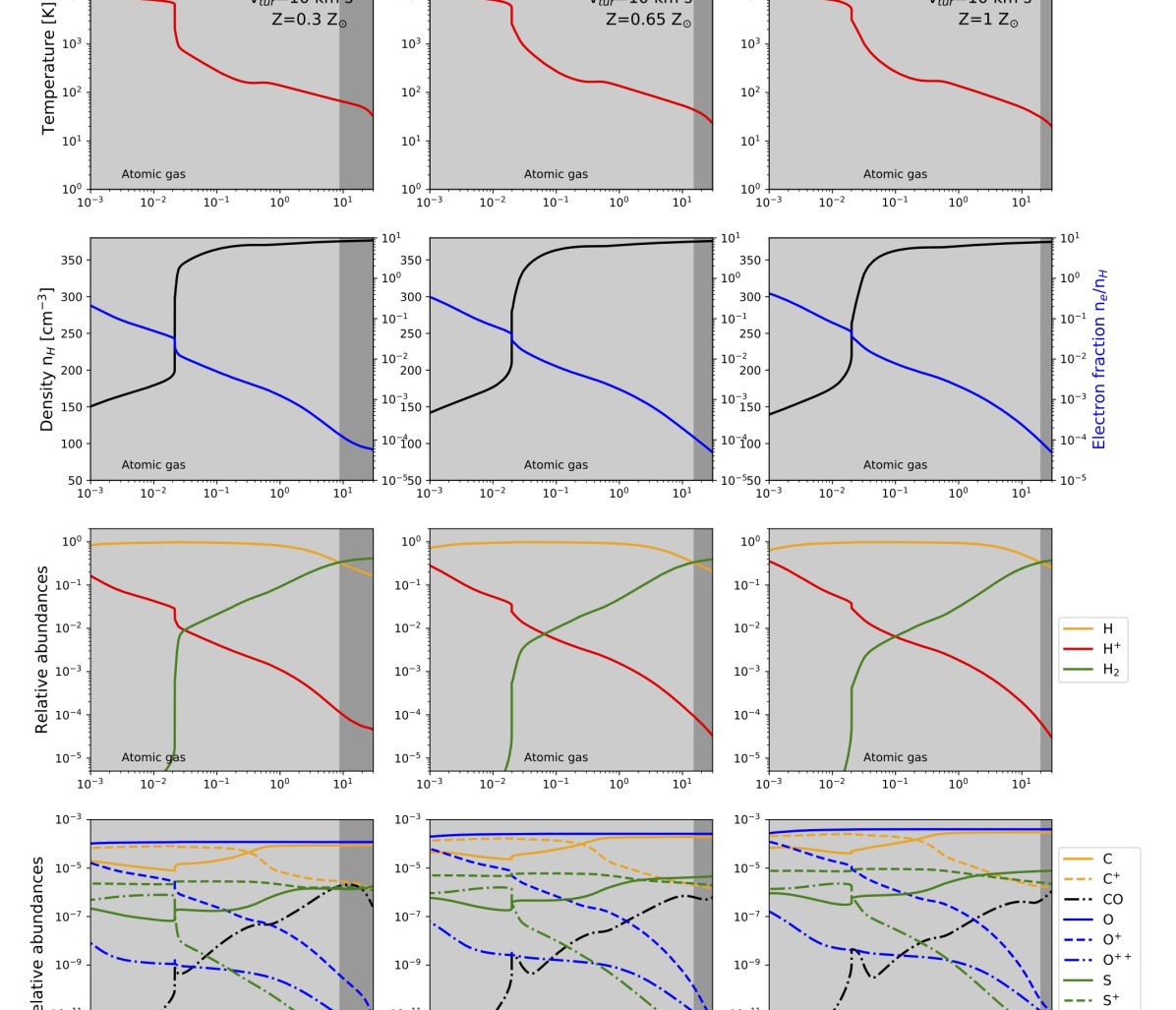
Figure 13: Same as Fig. 3, but this time G_Xis fixed at 10 and the metallicity varies: Z=0.3 Z_⊙ (left column), Z=0.65 Z_⊙ (central column) and Z= Z_⊙ (right column).

Appendix E Behavior of [O iii]$\lambda$ 5007 $\AA$/H${\beta}$, [N ii]$\lambda$ 6583 Å/H${\alpha}$ and [S ii]/H${\alpha}$ in the parameter space

.

Appendix F Predicted cumulative line emission

Table 6 presents the thirty brightest predicted line emission, from brightest to faintest, for the seven models described in the paper. The predicted line are for A_V=0.1, 1, 5 and 30 mag.

Table 6: Brightest predicted cumulative line emission.

Model			AV= 0.1		AV= 1		AV= 5		AV= 30
GX	vtur	Z	line	emission	line	emission	line	emission	line	emission
	km/s	Z⊙		erg s-1 cm-2		erg s-1 cm-2		erg s-1 cm-2		erg s-1 cm-2
0.1	10	1	[OI] 63$\mu$m	7.13e-06	[CI] 609$\mu$m	1.31e-05	[CI] 609$\mu$m	3.36e-05	[CI] 609$\mu$m	9.29e-05
			[C ii]$\lambda$ 157.7 $\mu$m	4.06e-06	[OI] 63$\mu$m	7.21e-06	H2 6.91$\mu$m	1.53e-05	[CI] 370$\mu$m	3.56e-05
			[CI] 609$\mu$m	3.24e-06	H2 6.91$\mu$m	5.65e-06	H2 5.5$\mu$m	1.37e-05	H2 6.9$\mu$m	2.51e-05
			[CI] 370$\mu$m	3.17e-06	H2 5.51$\mu$m	5.12e-06	H2 4.69$\mu$m	1.04e-05	H2 5.5$\mu$m	2.07e-05
			[SiII] 35$\mu$m	1.40e-06	[CI] 370$\mu$m	5.00e-06	H2 9.66$\mu$m	1.01e-05	H2 4.7$\mu$m	1.45e-05
			[NaI] 5890$\AA$	1.05e-06	H2 9.66$\mu$m	4.68e-06	[CI] 370$\mu$m	8.61e-06	CO 1300.05$\mu$m	1.18e-05
			H2 9.66$\mu$m	9.84e-07	[C ii]$\lambda$ 157.7 $\mu$m	4.23e-06	[OI] 63$\mu$m	7.36e-06	H2 9.66$\mu$m	1.06e-05
			[NaI] 5896$\AA$	9.31e-07	H2 4.69$\mu$m	3.96e-06	H2 17$\mu$m	7.21e-06	H2 17$\mu$m	1.05e-05
			H2 6.91$\mu$m	7.73e-07	H2 17$\mu$m	2.94e-06	H2 4.17$\mu$m	6.89e-06	H2 4.17$\mu$m	8.75e-06
			H2 17$\mu$m	7.11e-07	H2 4.17$\mu$m	2.68e-06	H2 1.74$\mu$m	5.24e-06	[OI] 63$\mu$m	7.65e-06
			H2 5.51$\mu$m	5.89e-07	H2 1.74$\mu$m	2.48e-06	H2 6.1$\mu$m	4.63e-06	H2 6.1$\mu$m	7.52e-06
			HI 6562.81$\AA$	5.43e-07	H2 3.84$\mu$m	1.80e-06	H2 3.84$\mu$m	4.53e-06	H2 8.02$\mu$m	6.46e-06
			[OI] 145$\mu$m	5.13e-07	H2 1.83$\mu$m	1.77e-06	H2 4.4$\mu$m	4.45e-06	CO 866.727$\mu$m	6.35e-06
			H2 4.69$\mu$m	4.30e-07	H2 4.4$\mu$m	1.72e-06	[C ii]$\lambda$ 157.7 $\mu$m	4.38e-06	H2 4.4$\mu$m	5.78e-06
			H2 12$\mu$m	3.28e-07	H2 6.1$\mu$m	1.71e-06	H2 8.0$\mu$m	4.34e-06	H2 5.05$\mu$m	5.64e-06
			H2 1.74$\mu$m	3.17e-07	H2 8.02$\mu$m	1.70e-06	H2 4.07$\mu$m	4.19e-06	H2 1.74$\mu$m	5.37e-06
			[FeII] 26$\mu$m	3.07e-07	H2 4.07$\mu$m	1.67e-06	H2 1.83$\mu$m	3.88e-06	H2 3.84$\mu$m	5.32e-06
			H2 8.02$\mu$m	2.92e-07	H2 3.83$\mu$m	1.57e-06	H2 3.83$\mu$m	3.86e-06	H2 4.95$\mu$m	5.19e-06
			[MgI] 2852$\AA$	2.86e-07	H2 1.12$\mu$m	1.48e-06	H2 5.05$\mu$m	3.83e-06	H2 4.07$\mu$m	4.85e-06
			H2 4.17$\mu$m	2.84e-07	H2 2.56$\mu$m	1.47e-06	H2 4.9$\mu$m	3.55e-06	H2 12$\mu$m	4.83e-06
10	10	1	[C ii]$\lambda$ 157.7 $\mu$m	3.85e-04	[C ii]$\lambda$ 157.7 $\mu$m	9.77e-04	[OI] 63$\mu$m	1.29e-03	[OI] 63$\mu$m	1.52e-03
			[OI] 63$\mu$m	2.86e-04	[OI] 63$\mu$m	8.22e-04	[C ii]$\lambda$ 157.7 $\mu$m	1.11e-03	H2 6.9$\mu$m	1.31e-03
			[SII] 6716$\AA$	1.15e-04	[SiII] 35$\mu$m	1.87e-04	[CI] 370$\mu$m	5.67e-04	[CI] 370$\mu$m	1.28e-03
			[CI] 9850$\AA$	1.14e-04	[CI] 370$\mu$m	1.40e-04	H2 6.9$\mu$m	2.55e-04	H2 5.5$\mu$m	1.17e-03
			[SiII] 35$\mu$m	1.08e-04	HI 6563$\AA$	1.26e-04	[CI] 609$\mu$m	2.54e-04	[C ii]$\lambda$ 157.7 $\mu$m	1.15e-03
			[OI] 6300$\AA$	8.69e-05	[CI] 9850$\AA$	9.79e-05	H2 5.5$\mu$m	2.39e-04	H2 4.7$\mu$m	8.77e-04
			HI 6563$\AA$	8.53e-05	[SII] 6716$\AA$	9.64e-05	[SiII] 35$\mu$m	2.01e-04	[CI] 609$\mu$m	5.85e-04
			[SII] 6731$\AA$	8.24e-05	[OI] 6300$\AA$	7.21e-05	H2 4.69$\mu$m	1.87e-04	H2 4.17$\mu$m	5.81e-04
			[NII] 6583$\AA$	6.52e-05	[SII] 6731$\AA$	6.89e-05	H2 9.66$\mu$m	1.57e-04	H2 9.66$\mu$m	4.27e-04
			[NeII] 13$\mu$m	6.25e-05	[NeII] 13$\mu$m	6.15e-05	H2 4.17$\mu$m	1.31e-04	H2 4.06$\mu$m	4.17e-04
			[OII] 3729$\AA$	6.07e-05	[OI] 145$\mu$m	5.62e-05	HI 6563$\AA$	1.20e-04	H2 17$\mu$m	4.14e-04
			[FeII] 5.3$\mu$m	4.70e-05	[NII] 6583$\AA$	5.44e-05	H2 3.83$\mu$m	9.48e-05	H2 3.83$\mu$m	4.09e-04
			[OII] 3726$\AA$	4.27e-05	[CI] 609$\mu$m	5.24e-05	H2 4.07$\mu$m	9.37e-05	H2 4.4$\mu$m	4.01e-04
			[CI] 9824$\AA$	3.81e-05	[OII] 3729$\AA$	4.92e-05	H2 3.84$\mu$m	9.12e-05	H2 3.84$\mu$m	3.84e-04
			[NI] 5200$\AA$	3.52e-05	[FeII] 5.3$\mu$m	4.59e-05	[SII] 6716$\AA$	8.73e-05	H2 6.1$\mu$m	3.60e-04
			[FeII] 1.2$\mu$m	3.36e-05	HI 4861$\AA$	3.78e-05	H2 4.4$\mu$m	8.72e-05	H2 5.05$\mu$m	3.08e-04
			[NeIII] 15$\mu$m	2.94e-05	[FeII] 25$\mu$m	3.57e-05	[CI] 9850$\AA$	8.63e-05	H2 4.3$\mu$m	3.05e-04
			[FeII] 1.6$\mu$m	2.87e-05	[OII] 3726$\AA$	3.47e-05	H2 17$\mu$m	8.16e-05	H2 4.9$\mu$m	2.95e-04
			HI 4861$\AA$	2.80e-05	[CI] 9824$\AA$	3.28e-05	H2 1.74$\mu$m	8.03e-05	H2 3.6$\mu$m	2.72e-04
			[OI] 6363$\AA$	2.78e-05	H2 6.9$\mu$m	3.26e-05	[OI] 145$\mu$m	7.73e-05	H2 8.02$\mu$m	2.67e-04

Table 7: Brightest cumulative predicted line emission.

Model			AV= 0.1		AV= 1		AV= 5		AV= 30
GX	vtur	Z	line	emission	line	emission	line	emission	line	emission
	km/s	Z⊙		erg s-1 cm-2		erg s-1 cm-2		erg s-1 cm-2		erg s-1 cm-2
100	10	1	[OII] 3729$\AA$	1.72e-03	[C ii]$\lambda$ 157.7 $\mu$m	4.41e-03	[OI] 63$\mu$m	1.26e-02	[OI] 63$\mu$m	1.92e-02
			[OII] 3726$\AA$	1.24e-03	[OI] 63$\mu$m	4.23e-03	[C ii]$\lambda$ 157.7 $\mu$m	7.11e-03	[C ii]$\lambda$ 157.7 $\mu$m	7.98e-03
			[NII] 6583$\AA$	1.20e-03	[SiII] 35$\mu$m	1.56e-03	[SiII] 35$\mu$m	3.32e-03	[SiII] 35$\mu$m	3.18e-03
			[OI] 6300$\AA$	8.22e-04	[OII] 3729$\AA$	1.46e-03	[NeII] 13$\mu$m	1.65e-03	H2 6.9$\mu$m	3.13e-03
			HI 6563$\AA$	7.91e-04	[NeII] 13$\mu$m	1.30e-03	[OII] 3729$\AA$	1.36e-03	[CI] 370$\mu$m	2.89e-03
			[SII] 6716$\AA$	7.05e-04	[SIII] 33$\mu$m	1.29e-03	[SIII] 33$\mu$m	1.23e-03	H2 5.5$\mu$m	2.65e-03
			[SIII] 9530$\AA$	5.93e-04	[OI] 6300$\AA$	1.23e-03	HI 6563$\AA$	1.10e-03	H2 4.69$\mu$m	1.95e-03
			[C ii]$\lambda$ 157.7 $\mu$m	5.53e-04	[NII] 6583$\AA$	1.18e-03	[OI] 6300$\AA$	1.07e-03	[OI] 145$\mu$m	1.48e-03
			[SIII] 33$\AA$	5.24e-04	[SII] 6716$\AA$	1.13e-03	[OI] 145$\mu$m	1.07e-03	[OII] 3729$\AA$	1.36e-03
			[SII] 6731$\AA$	5.12e-04	HI 6563$\AA$	1.08e-03	[NII] 6583$\AA$	1.05e-03	H2 4.17$\mu$m	1.31e-03
			[OI] 63$\mu$m	4.33e-04	[OII] 3726$\AA$	1.05e-03	[OII] 3726$\AA$	9.79e-04	H2 9.66$\mu$m	1.30e-03
			HeII 1640$\AA$	4.11e-04	[FeII] 5.3$\mu$m	9.33e-04	[SII] 6716$\AA$	9.70e-04	[NeII] 13$\mu$m	1.25e-03
			HeII 304$\AA$	4.11e-04	[SIII] 9530$\AA$	9.04e-04	[FeII] 5.3$\mu$m	8.93e-04	[OI] 6300$\AA$	1.06e-03
			[NII] 6548$\AA$	4.08e-04	[SII] 6731$\AA$	8.02e-04	[CI] 370$\mu$m	7.94e-04	[CI] 609$\mu$m	1.06e-03
			[NeII] 15$\mu$m	3.35e-04	[SIII] 19$\mu$m	7.09e-04	[SIII] 9530$\AA$	7.69e-04	[NII] 6583$\AA$	1.04e-03
			[CII] 2325$\AA$	3.30e-04	[NeIII] 15$\mu$m	6.85e-04	[FeII] 25$\mu$m	7.64e-04	HI 6563$\AA$	1.02e-03
			[SIII] 19$\mu$m	3.14e-04	[FeII] 1.2$\mu$m	5.44e-04	[SII] 6731$\AA$	6.90e-04	H2 3.8$\mu$m	1.01e-03
			[NI] 5200$\AA$	2.89e-04	[FeII] 1.6$\mu$m	4.83e-04	[NeIII] 15$\mu$m	6.90e-04	H2 4.06$\mu$m	1.00e-03
			[FeII] 5.3$\mu$m	2.86e-04	[NI] 5200$\AA$	4.70e-04	H2 9.66$\mu$m	6.89e-04	[SIII] 33$\mu$m	1.00e-03
			[SiII] 35$\mu$m	2.84e-04	[ArII] 7.0$\mu$m	4.67e-04	[SIII] 19$\mu$m	6.37e-04	[OII] 3726$\AA$	9.79e-04
10	0	1	[OI] 63$\mu$m	4.62e-04	[OI] 63$\mu$m	9.14e-04	[OI] 63$\mu$m	1.66e-03	[OI] 63$\mu$m	2.46e-03
			[CI] 9850$\AA$	1.49e-04	H2 1.21$\mu$m	4.79e-04	H2 2.12$\mu$m	1.08e-03	H2 4.69$\mu$m	1.49e-03
			[SII] 6716$\AA$	1.10e-04	H2 4.69$\mu$m	3.77e-04	H2 4.69$\mu$m	1.01e-03	H2 2.12$\mu$m	1.18e-03
			[C ii]$\lambda$ 157.7 $\mu$m	1.00e-04	H2 2.42$\mu$m	3.48e-04	H2 3.48$\mu$m	8.36e-04	H2 4.17$\mu$m	1.15e-03
			[OI] 6300$\AA$	8.12e-05	H2 3.48$\mu$m	3.20e-04	H2 2.42$\mu$m	8.28e-04	H2 3.48$\mu$m	1.13e-03
			[SII] 6731$\AA$	8.03e-05	H2 4.17$\mu$m	3.10e-04	H2 4.18$\mu$m	8.18e-04	H2 2.42$\mu$m	9.64e-04
			HI 6563$\AA$	5.44e-05	H2 2.40$\mu$m	2.85e-04	H2 2.40$\mu$m	6.97e-04	H2 3.6$\mu$m	8.73e-04
			H2 2.12$\mu$m	5.43e-05	H2 1.34$\mu$m	2.64e-04	H2 3.6$\mu$m	6.53e-04	H2 2.4$\mu$m	8.11e-04
			[NII] 6583$\AA$	5.21e-05	H2 3.6$\mu$m	2.52e-04	H2 2.8$\mu$m	6.29e-04	H2 2.8$\mu$m	7.94e-04
			[CI] 9824$\AA$	5.00e-05	H2 1.21$\mu$m	2.47e-04	H2 1.34$\mu$m	5.56e-04	H2 3.8$\mu$m	7.11e-04
			[SiII] 35$\mu$m	4.96e-05	H2 2.8$\mu$m	2.45e-04	H2 3.84$\mu$m	5.26e-04	H2 3.2$\mu$m	6.62e-04
			[OII] 3729$\AA$	4.47e-05	H2 3.8$\mu$m	2.03e-04	H2 3.23$\mu$m	5.08e-04	H2 8.0$\mu$m	6.11e-04
			H2 4.69$\mu$m	4.46e-05	H2 3.2$\mu$m	1.99e-04	H2 1.21$\mu$m	5.00e-04	H2 4.4$\mu$m	6.07e-04
			[NeII] 13$\mu$m	4.17e-05	H2 1.95$\mu$m	1.80e-04	H2 3.4$\mu$m	4.35e-04	H2 3.4$\mu$m	5.89e-04
			H2 3.48$\mu$m	3.98e-05	H2 3.4$\mu$m	1.72e-04	H2 4.4$\mu$m	4.14e-04	H2 1.34$\mu$m	5.51e-04
			[FeII] 5.3$\mu$m	3.97e-05	H2 9.66$\mu$m	1.71e-04	H2 1.95$\mu$m	3.40e-04	H2 6.1$\mu$m	5.25e-04
			H2 2.42$\mu$m	3.89e-05	H2 2.24$\mu$m	1.68e-04	H2 2.24$\mu$m	3.40e-04	H2 6.9$\mu$m	5.10e-04
			H2 4.17$\mu$m	3.82e-05	CO 325$\mu$m	1.59e-04	H2 9.66$\mu$m	3.96e-04	H2 2.24$\mu$m	4.49e-04
			H2 3.6$\mu$m	3.39e-05	H2 4.41$\mu$m	1.52e-04	H2 8.02$\mu$m	3.61e-04	H2 1.95$\mu$m	4.31e-04
			[NI] 5200$\AA$	3.34e-05	H2 8.0$\mu$m	1.50e-04	H2 6.9$\mu$m	3.22e-04	CO 260$\mu$m	4.26e-04

Table 8: Brightest predicted cumulative line emission.

Model			AV= 0.1		AV= 1		AV= 5		AV= 30
GX	vtur	Z	line	emission	line	emission	line	emission	line	emission
	km/s	Z⊙		erg s-1 cm-2		erg s-1 cm-2		erg s-1 cm-2		erg s-1 cm-2
10	50	1	[OII] 3729$\AA$	1.69e-04	[C ii]$\lambda$ 157.7 $\mu$m	7.28e-04	[C ii]$\lambda$ 157.7 $\mu$m	1.26e-03	[C ii]$\lambda$ 157.7 $\mu$m	1.42e-03
			[C ii]$\lambda$ 157.7 $\mu$m	1.35e-04	[OI] 63$\mu$m	2.94e-04	[OI] 63$\mu$m	8.05e-04	[OI] 63$\mu$m	1.16e-03
			[NII] 6583$\AA$	1.24e-04	[OII] 3729$\AA$	1.44e-04	[SiII] 35$\mu$m	2.85e-04	[CI] 370$\mu$m	5.52e-04
			[OII] 3726$\AA$	1.14e-04	[SIII] 33$\mu$m	1.35e-04	[NeII] 13$\mu$m	1.65e-04	[CI] 609$\mu$m	4.34e-04
			[OI] 6300$\AA$	8.41e-05	[SiII] 35$\mu$m	1.34e-04	[CI] 370$\mu$m	1.59e-04	[SiII] 35$\mu$m	2.79e-04
			HI 6563$\AA$	7.94e-05	[NII] 6583$\AA$	1.23e-04	[OII] 3729$\AA$	1.34e-04	H2 6.9$\mu$m	1.50e-04
			[SII] 6716$\AA$	7.53e-05	[OI] 6300$\AA$	1.21e-04	[SIII] 33$\mu$m	1.31e-04	H2 17$\mu$m	1.47e-04
			[SIII] 9531$\AA$	5.69e-05	[SII] 6716$\AA$	1.13e-04	H2 17$\mu$m	1.26e-04	[OII] 3729$\AA$	1.34e-04
			[SIII] 33$\mu$m	5.33e-05	[NeII] 13$\mu$m	1.11e-04	HI 6563$\AA$	1.11e-04	[NeII] 13$\mu$m	1.22e-04
			[SII] 6731$\AA$	5.22e-05	HI 6563$\AA$	1.07e-04	[NII] 6583$\AA$	1.09e-04	H2 5.5$\mu$m	1.11e-04
			[OI] 63$\mu$m	4.26e-05	[FeII] 5.3$\mu$m	9.93e-05	[CI] 609$\mu$m	1.09e-04	[NII] 6583$\AA$	1.08e-04
			[NII] 6548$\AA$	4.22e-05	[OII] 3726$\AA$	9.70e-05	H2 9.66$\mu$m	1.07e-04	[SIII] 33$\mu$m	1.07e-04
			HeII 1640$\AA$	3.83e-05	[SIII] 9531$\AA$	8.73e-05	[OI] 6300$\AA$	1.05e-04	[OI] 6300$\AA$	1.04e-04
			[NeIII] 15$\mu$m	3.38e-05	[SII] 6731$\AA$	7.80e-05	[FeII] 5.3$\mu$m	1.00e-04	HI 6563$\AA$	1.04e-04
			[FeII] 5.3$\mu$m	3.17e-05	[NeIII] 15$\mu$m	7.34e-05	[SII] 6716$\AA$	9.70e-05	H2 9.66$\mu$m	1.03e-04
			[SiII] 35$\mu$m	3.05e-05	[SIII] 19$\mu$m	7.11e-05	[OII] 3726$\AA$	9.08e-05	[OI] 145$\mu$m	9.73e-05
			[SIII] 19$\mu$m	3.01e-05	H2 9.66$\mu$m	6.22e-05	[NeIII] 15$\mu$m	8.03e-05	[SII] 6716$\AA$	9.59e-05
			HeII 304$\AA$	2.98e-05	[FeII] 1.2$\mu$m	5.58e-05	[SIII] 9531$\AA$	7.40e-05	[OII] 3726$\AA$	9.06e-05
			[NI] 5200$\AA$	2.98e-05	[FeII] 1.6$\mu$m	4.95e-05	[OI] 145$\mu$m	7.24e-05	[FeII] 5.3$\mu$m	7.73e-05
			[OI] 6364$\AA$	2.69e-05	[ArII] 7.0$\mu$m	4.71e-05	[FeII] 26$\mu$m	7.06e-05	H2 4.69$\mu$m	7.50e-05
10	10	0.3	[C ii]$\lambda$ 157.7 $\mu$m	3.71e-04	[C ii]$\lambda$ 157.7 $\mu$m	1.06e-03	H2 6.9$\mu$m	1.58e-03	H2 6.9$\mu$m	4.97e-03
			[OI] 63$\mu$m	2.65e-04	[OI] 63$\mu$m	7.46e-04	H2 5.5$\mu$m	1.53e-03	H2 5.5$\mu$m	4.51e-03
			HI 6563$\AA$	1.23e-04	H2 6.9$\mu$m	2.35e-04	[OI] 63$\mu$m	1.28e-03	H2 4.7$\mu$m	3.41e-03
			[SII] 6716$\AA$	7.28e-05	H2 5.5$\mu$m	2.27e-04	[C ii]$\lambda$ 157.7 $\mu$m	1.26e-03	H2 3.83$\mu$m	2.28e-03
			[SiII] 35$\mu$m	7.01e-05	H2 9.66$\mu$m	2.06e-04	H2 4.7$\mu$m	1.23e-03	H2 9.66$\mu$m	1.69e-03
			[OI] 6300$\AA$	6.08e-05	H2 4.7$\mu$m	1.85e-04	H2 9.66$\mu$m	9.79e-04	H2 17$\mu$m	1.69e-03
			[CI] 9850$\AA$	5.74e-05	H2 17$\mu$m	1.74e-04	H2 4.17$\mu$m	8.75e-04	[OI] 63$\mu$m	1.68e-03
			H2 9.66$\mu$m	5.69e-05	HI 6563$\AA$	1.70e-04	H2 3.83$\mu$m	6.93e-04	H2 4.4$\mu$m	1.66e-03
			H2 17$\mu$m	5.27e-05	H2 4.2$\mu$m	1.35e-04	H2 4.06$\mu$m	6.70e-04	[CI] 370$\mu$m	1.65e-03
			[SII] 6731$\AA$	5.13e-05	[SiII] 35$\mu$m	1.21e-04	H2 17$\mu$m	6.12e-04	H2 3.84$\mu$m	1.59e-03
			[NeII] 13$\mu$m	4.30e-05	[CI] 370$\mu$m	1.18-04	H2 3.84$\mu$m	6.07e-04	[C ii]$\lambda$ 157.7 $\mu$m	1.57e-03
			HI 4861$\AA$	3.96e-05	H2 3.83$\mu$m	1.17e-04	H2 4.4$\mu$m	6.01e-04	H2 6.1$\mu$m	1.51e-03
			[OII] 3729$\AA$	3.02e-05	H2 4.06$\mu$m	1.06e-04	[CI] 370$\mu$m	5.49e-04	H2 4.3$\mu$m	1.46e-03
			[NII] 6583$\AA$	2.90e-05	H2 1.7$\mu$m	9.98e-05	H2 1.7$\mu$m	5.07e-04	H2 4.9$\mu$m	1.27e-03
			H2 12$\mu$m	2.86e-05	H2 3.84$\mu$m	9.70e-05	H2 4.3$\mu$m	4.54e-04	H2 5.0$\mu$m	1.21e-03
			[FeII] 5.3$\mu$m	2.80e-05	H2 4.4$\mu$m	9.18e-05	H2 3.6$\mu$m	4.40e-04	H2 3.6$\mu$m	1.14e-03
			[NI] 5200$\AA$	2.66e-05	H2 3.6$\mu$m	7.34e-05	H2 4.9$\mu$m	4.04e-04	H2 8.0$\mu$m	1.10e-03
			[OI] 145$\mu$m	2.23e-05	H2 4.3$\mu$m	7.05e-05	H2 6.1$\mu$m	3.71e-04	H2 4.4$\mu$m	1.10e-03
			[FeII] 1.2$\mu$m	2.12e-05	H2 1.12$\mu$m	6.89e-05	H2 3.48$\mu$m	3.47e-04	H2 3.48$\mu$m	9.31e-04
			[OII] 3726$\AA$	2.12 e-05	[SII] 6716$\AA$	6.07e-05	H2 2.5$\mu$m	3.45e-04	H2 3.4$\mu$m	8.57e-04

Table 9: Brightest predicted cumulative line emission.

Model			AV= 0.1		AV= 1		AV= 5		AV= 30
GX	vtur	Z	line	emission	line	emission	line	emission	line	emission
	km/s	Z⊙		erg s-1 cm-2		erg s-1 cm-2		erg s-1 cm-2		erg s-1 cm-2
10	10	0.65	[C ii]$\lambda$ 157.7 $\mu$m	3.81e-04	[C ii]$\lambda$ 157.7 $\mu$m	1.01e-03	[OI] 63$\mu$m	1.28e-03	H2 6.9$\mu$m	2.20e-03
			[OI] 63$\mu$m	2.82e-04	[OI] 63$\mu$m	7.98e-04	[C ii]$\lambda$ 157.7 $\mu$m	1.16e-03	H2 5.5$\mu$m	1.98e-03
			[SII] 6716$\AA$	9.84e-05	[SiII] 35$\mu$m	1.60e-04	[CI] 370$\mu$m	5.62e-04	[OI] 63$\mu$m	1.55e-03
			HI 6563$\AA$	9.82e-05	HI 6563$\AA$	1.41e-04	H2 6.9$\mu$m	5.14e-04	H2 4.69$\mu$m	1.49e-03
			[SiII] 35$\mu$m	9.31e-05	[CI] 370$\mu$m	1.32e-04	H2 5.5$\mu$m	4.89e-04	[CI] 370$\mu$m	1.39e-03
			[CI] 9850$\AA$	9.08e-05	[SII] 6716$\AA$	8.22e-05	H2 4.7$\mu$m	3.86e-04	[C ii]$\lambda$ 157.7 $\mu$m	1.22e-03
			[OI] 6300$\AA$	7.82e-05	[CI] 9850$\AA$	7.83e-05	H2 9.66$\mu$m	3.19e-04	H2 4.17$\mu$m	9.88e-04
			[SII] 6731$\AA$	6.70e-05	H2 6.9$\mu$m	6.70e-05	H2 4.2$\mu$m	2.74e-04	H2 9.66$\mu$m	7.28e-04
			[NeII] 13$\mu$m	5.41e-05	[OI] 6363$\AA$	6.50e-05	[CI] 609$\mu$m	2.52e-04	H2 4.06$\mu$m	7.18e-04
			[NII] 6583$\AA$	5.06e-05	H2 9.66$\mu$m	6.19e-05	H2 3.83$\mu$m	2.04e-04	H2 3.83$\mu$m	7.09e-04
			[OII] 3729$\AA$	5.05e-05	[SII] 6731$\AA$	5.84e-05	H2 4.06$\mu$m	1.99e-04	H2 17$\mu$m	7.05e-04
			[FeII] 5.3$\mu$m	3.81e-05	H2 5.5$\mu$m	5.82e-05	H2 3.84$\mu$m	1.90e-45	H2 4.4$\mu$m	6.85e-04
			[OII] 3726$\AA$	3.56e-05	[OI] 145$\mu$m	5.46e-05	H2 4.4$\mu$m	1.83e-04	H2 3.84$\mu$m	6.55e-04
			[NI] 5200$\AA$	3.26e-05	[NeII] 13$\mu$m	5.32e-05	[SiII] 35$\mu$m	1.75e-04	[CI] 609$\mu$m	6.12e-04
			HI 4861$\AA$	3.19e-05	[CI] 609$\mu$m	5.05e-05	H2 17$\mu$m	1.74e-04	H2 6.1$\mu$m	5.94e-04
			[CI] 9824$\AA$	2.38e-05	H2 4.69$\mu$m	4.54e-05	H2 1.74$\mu$m	1.62e-04	H2 4.3$\mu$m	5.21e-04
			[FeII] 1.2$\mu$m	2.39e-05	HI 4861$\AA$	4.23e-05	H2 3.6$\mu$m	1.340e-04	H2 5.05$\mu$m	5.12e-04
			H2 9.66$\mu$m	2.32e-05	H2 17$\mu$m	4.24e-05	H2 4.3$\mu$m	1.37e-04	H2 4.9$\mu$m	5.00e-04
			[OI] 6363$\AA$	2.24e-05	[NII] 6583$\AA$	4.23e-05	HI 6563$\AA$	1.34e-04	H2 3.6$\mu$m	4.63e-04
			[OI] 145$\mu$m	2.21e-05	[OII] 3729$\AA$	4.09e-05	H2 6.1$\mu$m	1.31e-04	H2 8.0$\mu$m	4.38e-04