Optical phonons coupled to a Kitaev spin liquid

Abstract

Emergent excitation continua in frustrated magnets are a fingerprint of fractionalization, characteristic of quantum spin-liquid states. Recent evidence from Raman scattering for a coupling between such continua and lattice degrees of freedom in putative Kitaev magnets [1, 2, 3, 4, 5, 6] may provide insight into the nature of the fractionalized quasiparticles. Here we study the renormalization of optical phonons coupled to the underlying $\mathbb{Z}_{2}$ quantum spin-liquid. We show that phonon line-shapes acquire an asymmetry, observable in light scattering, and originating from two distinct sources, namely the dispersion of the Majorana continuum and the Fano effect. Moreover, we find that the phonon life-times increase with increasing temperature due to thermal blocking of available phase space. Finally, in contrast to low-energy probes, optical phonon renormalization is rather insensitive to thermally excited gauge fluxes and barely susceptible to external magnetic fields.

Introduction.– There is an ongoing pursuit of the signatures of the elusive quantum spin-liquid (QSL) state of matter [7, 8, 9]. The difficulty to identify such states is due to the fact that they do not break any symmetries and lack conventional local order parameters of magnetic or related nature down to zero temperature. Recently, QSLs with a $\mathbb{Z}_{2}$ gauge structure may have actually come close to material realization, motivated by the exact solution of the famous Kitaev spin model (KSM) with compass-exchange on the two-dimensional (2D) honeycomb lattice [10]. In this model, spins fractionalize into static $\mathbb{Z}_{2}$ gauge fluxes and itinerant Majorana fermions, with a gapless QSL ground state. In external magnetic fields the KSM opens a gap and displays chiral Majorana edge-modes. Variants and generalizations of the KSM in 1D [11, 12, 13, 14, 15, 16, 17], 2D [18], and 3D [19, 20, 21], as well as for spins larger than $1/2$ [22, 23, 24] have been considered.

Mott-insulators with strong spin-orbit coupling (SOC) are promising materials to realize the KSM [25, 26, 27, 28]. However, residual non-Kitaev exchange interactions remain an issue, with all current systems under consideration eventually displaying magnetic order at low temperatures. From a present perspective [29, 30, 31, 32, 9], $\alpha$-RuCl₃, either above its ordering temperature, or with magnetic order suppressed by external magnetic fields, is one of the prime candidates under scrutiny for $\mathbb{Z}_{2}$ QSL physics. Recent thermal Hall effect measurements in $\alpha$-RuCl₃, suggest half-integer quantization plateaus [33] which are consistent with Majorana edge states, including a field-angular variation of the topological Chern number identical to that of the Kitaev QSL [34], and a bulk-boundary correspondence claimed in specific heat measurements [35]. In addition to edge transport, a multitude of bulk spectroscopic probes have been invoked, aiming to identify continua characteristic of the fractional Majorana excitations. This pertains to inelastic neutron scattering [36, 37, 38, 39, 40, 41] and local resonance techniques [42, 43], as well as to magnetic Raman scattering [44, 45, 46].

An interesting open question is whether the coupling of Majorana fermions of the putative KSM to other degrees of freedom can be used to provide signatures of their existence. Coupling to phonons [47, 48, 49, 50] can induce characteristic renormalizations, examples of which seem to have been observed recently for acoustic phonons [51]. Regarding optical phonons, Raman scattering [1, 2, 3, 4, 5, 6] has provided early on evidence for Raman active phonons with Fano line-shapes, overlapping with the magnetic Raman continuum [44, 45]. This has been speculated to be a signature of renormalization of optical phonons by Majorana fermions but up to now a microscopic description was missing.

Here, we provide a theory of optical phonons and coupled to a KSM. We describe the microscopic details of the coupling and evaluate the phonon self-energy. The phonon renormalization versus energy and temperature is studied, the relative importance of Majorana and flux excitations is discussed, and the implications for Raman scattering are clarified. We find convincing qualitative agreement with experimental data, which points to an intriguing interpretation of a Majorana scattering induced optical phonon renormalization in the candidate material $\alpha$-RuCl₃.

Optical-phonon Majorana mixing.– Here, we consider phonons of a 2D Honeycomb lattice coupled magnetoelastically to the Kitaev QSL. The total Hamiltonian of the system reads $H=H_{P}+H_{K}+H_{KP}$ where $H_{P}$ stands for the quadratic free phonon contribution $H_{P}=\sum_{\mathbf{q}m}\left(\omega_{m\mathbf{q}}+\frac{1}{2}\right)b_{m\mathbf{q}}^{\dagger}b_{m\mathbf{q}}$ with $b_{m\mathbf{q}}^{\dagger}$, $b_{m\mathbf{q}}$ being bosonic creation annihilation operators, respectively, at momentum $\mathbf{q}$ for the mode $m$, and $\omega_{m\mathbf{q}}$ the corresponding energy.

The magnetic degrees of freedom are described by the Kitaev spin Hamiltonian $H_{K}=\sum_{\mathbf{r},\bm{\delta}}J_{\bm{\delta}}S_{\mathbf{r}}^{d_{\bm{\delta}}}S_{\mathbf{r}-\bm{\delta}}^{d_{\bm{\delta}}}$, [10] (see also Fig. 1). $\mathbf{r}=l_{1}\mathbf{a}_{1}+l_{2}\mathbf{a}_{2}$, with $l_{1,2}=0,1,\ldots,L-1$, refers to a triangular Bravais lattice of linear dimension $L$, and $\bm{\delta}$ sets the location of the basis of the honeycomb lattice, with $N=2L^{2}$ sites. The components $d_{\bm{\delta}}$ of the spin-1/2 operators $S$ assume the values $d_{\bm{\delta}}=x,y,z$ depending on the $\bm{\delta}$-vector, while $J_{\bm{\delta}}$ are the Kitaev interactions. We consider the isotropic case $J_{\bm{\delta}}=J$ and set $\hbar,k_{B}=1$.

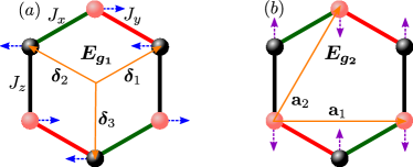
Figure 1: Kitaev Hexagons with compass magnetic interactions $J_{x,y,z}$ along the directions $\bm{\delta}_{1}=\frac{a}{2}(+\sqrt{3}\bm{e}_{x}+\bm{e}_{y})$, $\bm{\delta}_{2}=\frac{a}{2}(-\sqrt{3}\bm{e}_{x}+\bm{e}_{y})$, and $\bm{\delta}_{3}=-a\bm{e}_{y}$, respectively. In addition the lattice vectors of the triangular Bravais lattice are shown $\mathbf{a}_{1}=a\sqrt{3}\bm{e}_{x}$, $\mathbf{a}_{2}=\frac{a\sqrt{3}}{2}(\bm{e}_{x}+\sqrt{3}\bm{e}_{y})$. The distortion of the lattice due to the two optical modes $E_{g_{1}}(a)$ and $E_{g_{2}}(b)$ is indicated by the small blue and purple arrows, respectively, with a dashed shaft.

Following the literature [10, 12], we map the spin model onto one for two species of Majorana fermions $c$ and $\bar{c}$, with $\{c_{i},c_{j}\}=2\delta_{ij}=\{\bar{c}_{i},\bar{c}_{j}\}$ and $\{c_{i},\bar{c}_{j}\}=0$. This mapping renders Majorana fermions of, e.g., $c$-type itinerant, while the other type pairs into a static $\mathbb{Z}_{2}$ gauge fields $\eta=\pm 1$ along, e.g., the $\bm{\delta}_{3}$ direction. The gauge field generates a conserved flux, equivalent to a macroscopic number of conserved local operators in the spin language [10, 52]. In the Majorana representation, $H_{K}$ reads

$$H_{K}=J\sum_{\mathbf{r},\bm{\delta}}h_{\bm{\delta}}(\mathbf{r})~{},~{}~{}h_{\bm{\delta}}(\mathbf{r})=-\frac{i}{4}\eta_{\bm{\delta}}(\mathbf{r})c_{\mathbf{r}}c_{\mathbf{r}-\bm{\delta}}^{\prime}~{},$$ (1)

where the gauge field $\eta_{\bm{\delta}}$ acquires the values $\eta_{\bm{\delta}_{1}}(\mathbf{r})=\eta_{\bm{\delta}_{2}}(\mathbf{r})=1$, and $\eta_{\bm{\delta}_{3}}(\mathbf{r})=\pm 1$. Primed Majorana fermions reside on the basis sites. The ground state resides within the uniform gauge sector, which is separated from other sectors by a gap $\Delta\approx 0.065J$. At finite temperature $T$ fluxes become thermally excited and proliferate in a narrow range near a very low $T^{*}\approx 0.012J$. For several observables the emergent disorder introduced by the visons has been shown to be of physical significance [14, 53, 54, 49]. For the present case of interest, i.e., optical phonons, we show that gauge excitations imply only negligible quantitative modifications.

We focus on magnetoelastic coupling between spins and lattice degrees of freedom, i.e., on the leading order variation $J(\mathbf{u}_{\mathbf{r}}-\mathbf{u}_{\mathbf{r}-\bm{\delta}}^{\prime})\approx J+\nabla J\cdot(\mathbf{u}_{\mathbf{r}}-\mathbf{u}_{\mathbf{r}-\bm{\delta}}^{\prime})$ of the exchange with respect to lattice deformations $\mathbf{u}_{\mathbf{r}}$ at site ${\bf r}$. The lattice distortions in Fourier space, $\mathbf{u}_{\mathbf{q}}^{(\prime)}=\sum_{\mathbf{r}}e^{-i\mathbf{q}\cdot[\mathbf{r}(+\bm{\delta}_{1})]}\mathbf{u}_{\mathbf{r}}^{(\prime)}/\sqrt{N}$, are quantized in terms of phonon normal modes $\mathbf{u}_{\mathbf{q}}^{(\prime)}=\sum_{m}(\gamma_{m\mathbf{q}}^{x(\prime)}\hat{e}_{x}+\gamma_{m\mathbf{q}}^{y(\prime)}\hat{e}_{y})/\sqrt{2M\omega_{m\mathbf{q}}}\hphantom{a}\mathcal{B}_{m\mathbf{q}}$, with $\mathcal{B}_{m\mathbf{q}}=b_{m\mathbf{q}}+b_{m,-\mathbf{q}}^{\dagger}$ comprising the annihilation and creation operators of mode $m$ at momentum $\pm\mathbf{q}$ and energy $\omega_{m\mathbf{q}}$ with coefficients of the polarization vectors $\gamma$ and $\gamma^{\prime}$ and $M$ is of the order of the ruthenium mass. Using this, the Majorana phonon coupling reads

$$H_{KP}=\sum_{m\mathbf{q}}\mathcal{B}_{m\mathbf{q}}\mathcal{H}_{m,-\mathbf{q}}~{},~{}~{}\mathcal{H}_{m\mathbf{q}}=\sum_{\bm{\delta}}\Lambda_{m\mathbf{q}}^{\bm{\delta}}h_{\bm{\delta};\mathbf{q}},$$ (2)

where the form factor of the coupling is encoded in $\Lambda_{m\mathbf{q}}^{\bm{\delta}}$.

While Eq. (2) applies to acoustic, as well as to optical phonons, we focus on the $E_{g_{1}}$ and $E_{g_{2}}$ optical modes, observed in Raman experiments. These are of particular interest, since allegedly, they overlap with the Majorana continuum. For Raman scattering it is safe to consider $q\rightarrow 0$ only and we drop all $\mathbf{q}$-labels hereafter. In the supplemental material we treat also $q\neq 0$ (and moreover weak magnetic fields) [55]. The phonon energies are $\omega_{1}\equiv\omega_{g_{1}}\approx 116cm^{-1}\approx 1.9J$ and $\omega_{2}\equiv\omega_{g_{2}}\approx 165cm^{-1}\approx 2.6J$, where we assume a Kitaev coupling of $J\approx 90K$. The vibrational pattern of the two modes [2] is shown in Fig. 1. In terms of Eq. (2) the lattice modulations imply $\bm{\Lambda}_{m}=\Lambda_{m}[1,-1^{m},\lambda_{m}]$, with $m=1,2$, and $\lambda_{m}$ denotes a possible anisotropy between the $\bm{\delta}_{1,2}$ and $\bm{\delta}_{3}$ directions. The magnitude of $\Lambda_{m}$ can be assumed to be in the perturbative regime [49]. Note, a detailed microscopic derivation of the spin-phonon coupling including the effect of spin-orbit effects beyond the pure Kitaev model is given in the supplementary material [55], see also Refs. [56, 57, 58].

The coupling of the phonons to the fractionalized magnetic excitations, Eq. (2), leads to a renormalization of the bare phonon propagators, $D_{m}^{0}(z)=2\omega_{m}/(z^{2}-\omega_{m}^{2})$, with $z=\omega+i0^{+}$, the frequency dependence. The dressed phonon propagators can then be determined by the $2\times 2$ self-energy matrix $\bm{\Sigma}(z)$ and the corresponding Dyson’s equation,

$$\mathbf{D}(z)\approx[\mathbf{D}_{0}^{-1}(z)-\bm{\Sigma}(z)]^{-1},~{}\bm{\Sigma}_{mm^{\prime}}=\langle\langle\mathcal{H}_{m};\mathcal{H}_{m^{\prime}}^{\dagger}\rangle\rangle,$$ (3)

with $[\mathbf{D}_{0}(z)]_{mm^{\prime}}=\delta_{mm^{\prime}}D_{m}^{0}(z)$ while the double brackets denote the Green’s function. A central goal of the paper is to evaluate the self-energy in Eq. (3). We do this in two ways: first analytically, assuming a uniform gauge field configuration in Eq. (1), and second numerically by considering a numerical random averaging over disordered configurations of the gauge field $\eta$. While the former approach is justified at temperatures ranging from 0 up to $T^{*}$, the latter is valid at temperatures higher than the flux gap $T\gtrsim\Delta$ [53, 54, 49].

Phonon self-energy: uniform gauge.– At low temperatures, $T\lesssim T^{*}$, it can be assumed, that the system acquires a uniform gauge configuration, $\eta_{\bm{\delta}}=1$, allowing for the analytical calculation of the phonon self-energy. First, the Kitaev terms in Eq. (1) can be brought to a diagonal form by going to reciprocal space $\mathbf{k}=k_{1}\mathbf{G}_{1}+k_{2}\mathbf{G}_{2}$, where $\mathbf{G}_{1}=\frac{1}{3a}(\sqrt{3}\bm{e}_{x}-\bm{e}_{y})$ and $\mathbf{G}_{2}=\frac{2}{3a}\bm{e}_{y}$ are the reciprocal lattice vectors, i.e., $\mathbf{a}_{i}\cdot\mathbf{G}_{j}=\delta_{i,j}$ for $i(j)=1,2$. The coefficients $k_{1,2}$ are set to antiperiodic boundary conditions $k_{j}=2\pi(l_{j}+\frac{1}{2})/L$, to allow all Majoranas to pair into complex fermions. The Fourier transform of the Majoranas reads $c_{\mathbf{k}}=\sum_{\mathbf{r}}e^{-i\mathbf{k}\cdot\mathbf{r}}c_{\mathbf{r}}/\sqrt{2N}$ such that $\{c_{\mathbf{k}},c_{\mathbf{k}^{\prime}}^{\dagger}\}=\delta_{\mathbf{k},\mathbf{k}^{\prime}}$, and similarly for the $c^{\prime}$ operators.

In the diagonal complex fermion basis, $\Psi_{\mathbf{k}}^{\dagger}=(d_{1,\mathbf{k}}^{\dagger},d_{2,\mathbf{k}}^{\dagger})$, $H_{K}$ and $\mathcal{H}_{m}$ of Eq. (1) and (2) read $H_{K}=\frac{1}{2}\sum_{\mathbf{k}}\Psi_{\mathbf{k}}^{\dagger}E_{\mathbf{k}}\Psi_{\mathbf{k}}$ and $\mathcal{H}_{m}=\frac{1}{2}\sum_{\mathbf{k}}\Psi_{\mathbf{k}}^{\dagger}V_{m;\mathbf{k}}\Psi_{\mathbf{k}}$ with

$$E_{\mathbf{k}}=\left(\begin{array}[]{cc}\epsilon_{\mathbf{k}}&0\\ 0&-\epsilon_{\mathbf{k}}\end{array}\right),\hphantom{aa}V_{m;\mathbf{k}}=\left(\begin{array}[]{cc}g_{m;\mathbf{k}}^{\prime}&ig_{m;\mathbf{k}}^{\prime\prime}\\ -ig_{m;\mathbf{k}}^{\prime\prime}&-g_{m;\mathbf{k}}^{\prime}\end{array}\right).$$ (4)

The energy eigenvalues are given by $\epsilon_{\mathbf{k}}=|f_{\mathbf{k}}|=\frac{J}{2}[3+2\cos k_{1}+2\cos k_{2}+2\cos(k_{1}-k_{2})]^{1/2}$, with $f_{\mathbf{k}}=J\sum_{\bm{\delta}}t_{\bm{\delta};\mathbf{k}}$, and $t_{\bm{\delta};\mathbf{k}}=-\frac{i}{2}e^{-i\mathbf{k}\cdot\bm{\delta}}$. The real ($g^{\prime}$) and imaginary part ($g^{\prime\prime}$) of the function $g$ of the scattering matrix $V$ are given by $g_{m;\mathbf{k}}=(f_{\mathbf{k}}^{*}/\epsilon_{\mathbf{k}})\sum_{\bm{\delta}}\Lambda_{m}^{\bm{\delta}}t_{\bm{\delta};\mathbf{k}}/\sqrt{N}$.

The evaluation of the self energy using (3) and (4) is straightforward. In that process and due to $c_{\mathbf{k}}^{\dagger}=c_{-\mathbf{k}}$, anomalous commutators $\{d_{1,\mathbf{k}},d_{2,\mathbf{k}^{\prime}}\}=\delta_{\mathbf{k},-\mathbf{k}^{\prime}}$ and their corresponding contractions arise, implying also a time evolution $d_{j,\mathbf{k}}(t)=d_{j,\mathbf{k}}e^{\mp i\epsilon_{\mathbf{k}}t}$ for $j=1,2$, respectively. Thus, the self-energy exhibits particle-hole (ph) and particle-particle (pp) absorption channels, the amplitudes of which are determined via the diagonal and off-diagonal matrix elements of the matrix $V$. In the $q=0$ limit, considered here, the ph-channel vanishes. The pp-scattering-amplitudes acquire simple forms, and all diagonal and off-diagonal self-energies are described by a single function

$$\bm{\Sigma}(z)=\left(\begin{array}[]{cc}a_{1}&b\\ b&a_{2}\end{array}\right)\Sigma(z),\hphantom{a.}\Sigma(z)=\frac{1}{N}\sum_{\mathbf{k},\pm}A_{\mathbf{k}}^{2}\frac{1-2f_{\mathbf{k}}}{2\epsilon_{\mathbf{k}}\mp z},$$ (5)

with the matrix elements $a_{1}=\Lambda_{1}(3+\lambda_{1}^{2})/\Lambda_{2}$, $a_{2}=\Lambda_{2}(1-\lambda_{2})^{2}/\Lambda_{1}$, and $b=\lambda_{1}(1-\lambda_{2})$, the scattering amplitude $A_{\mathbf{k}}=\Lambda_{1}\Lambda_{2}\cos(k_{x}a/2)\sin(\sqrt{3}k_{y}a/2)/(2\epsilon_{\mathbf{k}})$, and the Fermi-Dirac distribution $f_{\mathbf{k}}=1/(e^{\epsilon_{\mathbf{k}}/T}+1)$. Two special cases arise. For $\lambda_{2}=1$ the $E_{g_{2}}$ spin phonon Hamiltonian satisfies $\mathcal{H}_{2}\propto H_{K}$, leading to no scattering for that mode. For $\lambda_{1}=0$, symmetry prevents mixing of the $E_{g_{1}}$ and $E_{g_{2}}$ modes.

Phonon self-energy: random gauge.– For temperatures $T\gtrsim 0.1\dots 0.2J\gg T^{*}$, thermal gauge excitations need to be taken into account. For that, a random averaging over maximally disordered configurations of $\eta_{\bm{\delta}_{3}}(\mathbf{r})$ is sufficient to describe the fermionic system’s properties. As this breaks translational invariance, we resort to a numerical real-space evaluation of the defect-averaged self-energy $\bm{\Sigma}(z)$. This approach has been detailed in Refs. [49, 53] and is recapitulated in [55].

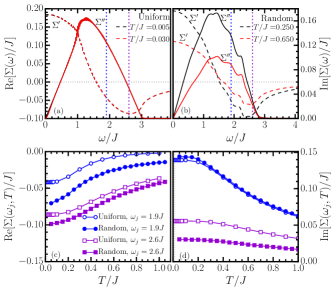
Figure 2: Panels (a) and (b): Frequency dependence of the self-energy $\Sigma$ for two temperatures in the (a) uniform gauge field sector for $L=200$ (curves overlap) and (b) averaged over $N_{R}=200$ maximally disordered sectors, on lattices of $L=30$, with $\Lambda_{1,2}/J=1$. Dashed blue(purple) lines at $\omega_{j}/J=1.9(2.6)$ on both panels indicate the position of the phonon modes $E_{g_{1}}$($E_{g_{2}}$). The scale of $\Sigma^{\prime}$, for both uniform or random sectors, is indicated on the left side of panel (a) while the scale of $\Sigma^{\prime\prime}$ is shown on the right side of panel (b). Panels (c) and (d): Temperature dependence of the real and imaginary parts of $\Sigma$, respectively, at the phonon frequencies $\omega/J=1.9$ (blue circles) and $\omega/J=2.6$ (purple squares). Open(Filled) symbols indicate results acquired for uniform(random) gauge-field configuration(s).

Phonon self-energy: results.– In Fig. 2, we present results for the self-energy $\Sigma$ versus frequency and temperature, for both homogeneous as well as random gauge states. In Fig. 2(a), we plot $\Sigma(\omega)$ obtained from the analytical approach for two temperatures, $T=0.005J<T^{*}$ and $T=0.030J\gtrsim T^{*}$ (curves overlap). Calculations are performed on lattices with $L=200$. For $\omega<0$, analyticity requires $(-)\Sigma^{\prime(\prime\prime)}(-\omega)=\Sigma^{\prime(\prime\prime)}(\omega)$ for the real(imaginary) part [left(right) $y$-axis of panel [a(b)]]. Both, $\Sigma^{\prime}$ and $\Sigma^{\prime\prime}$, contribute to the renormalization of the $E_{g_{1}}$ and $E_{g_{2}}$ phonons, the energy of which is marked with a blue and purple dotted line, respectively. Since $\Sigma^{\prime}(\omega_{j},T)<0$ at both anticipated phonon energies $\omega_{j}$, a downward renormalization will occur. Most importantly however, regarding their life time, both phonons reside in a range of negative slope of $\Sigma^{\prime\prime}$ versus $\omega$. Therefore the life time will be dispersive, with phonon spectral functions that display asymmetric line shapes with enhanced left-broadening.

Regarding the gauge excitations, Fig. 2(b) shows $\Sigma$ from the numerical approach for $T\gg T^{\star}$ on lattices of $L=30$, averaging over $N_{R}=200$ maximally disordered gauge field configurations. First, the overall shape of $\Sigma$ displays no qualitative change compared to Fig. 2(a), with only some additional fine structure arising from the gauge-field excitations. Second however, there is a reduction of the bandwidth to $<3J$, which affects the scattering of the high frequency mode $E_{g_{2}}$. Finally, there is clearly visible reduction of $\Sigma$ with increasing $T$. This is dictated by the Fermi-function (as in Eq. (5)) reducing the available phase space. For the low-$T$ results of Fig. 2(a) this effect is too small to be observable.

In Figs. 2(c) and (d), we scan the temperature dependence of the real and imaginary part of the self-energy, respectively, at the two frequencies of the phonon modes. In doing so, we plot results obtained from both, the analytical and the numerical approach - even though in principle the former is applied for temperatures beyond its validity. This figure clearly demonstrates, that for the renormalization of optical phonons gauge-field excitations yield only small quantitative corrections. For the rest of the paper, we therefore remain in the uniform gauge configuration.

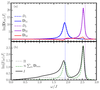
Figure 3: (a) Frequency dependence of the phonon spectral weight as evaluated via Eq. (3) using Eq. (5) for $\Lambda_{1(2)}/J=0.3(0.9)$, $\lambda_{1,2}=2$, and $T=0.005J$. Dashed lines represent the decoupled phonon modes $D_{m}$. (b) Frequency dependence of the total Raman intensity $I$ (black solid line), evaluated via Eq. (6) for the same $\bm{\Lambda}$’s as for panel (a) and $r_{m}=0.3$, $C_{m}=-0.8J$. For comparison, the diagonal phonon spectral weight $\sum_{m}\mathbf{D}_{mm}(\omega)$ is plotted (green dashed line), here rescaled by a factor of $1/8$ for visual reasons, as well as the fermionic Raman response, $\sim\Pi(\omega)$ (gray dashed line).

Next we discuss the renormalized optical phonon modes, obtained from the $2\times 2$ Dyson equation Eq. (3) using $\bm{\Sigma}$ from Eq. (5). In general, because of $b\neq 0$, phonon mixing by virtue of the fermionic background will occur, i.e. $\mathbf{D}_{mm}\neq[D_{m}^{0}-a_{m}\Sigma]^{-1}\equiv D_{m}$. However, we will stay in the perturbative regime $b\Sigma((\omega_{2}+\omega_{1})/2)/(\omega_{2}-\omega_{1})\ll 1$, where the mixing is weak and can be ignored. Fig. 3(a) depicts the individual (off)diagonal phonon spectra $D^{\prime\prime}_{mn}(\omega)$ for intermediate $\Lambda_{1}(\Lambda_{2})=0.3J(0.9J)$, $\lambda_{1,2}=2$ and for $T=0.005J$. First, both diagonal elements of $\mathbf{D}$ exhibit the anticipated downward renormalization with respect to $\omega_{m}$, largest for $E_{g_{2}}$. In accordance with Fig. 2(c), the modes’ peaks will shift upwards to $\omega_{m}$ as the temperature is increased. Second, the frequency dependence of $\Sigma^{\prime\prime}(\omega)$ leads to slightly asymmetric phonon line shapes. We emphasize, that this asymmetry is not related to the Fano effect [59], commonly cited in such cases. The width of the phonon mode is expected to shrink as the temperature is increased, Fig. 2(d). I.e., in contrast to most conventional excitations in many-body systems, their life-time grows with temperature. Third, the phonon mixing is rather weak, i.e., $\mathbf{D}_{12}\ll\mathbf{D}_{11(22)}$ and $\mathbf{D}_{mm}\approx D_{m}$, essentially rendering the two phonon modes decoupled.

Raman response and Fano-lineshape.– Finally, we speculate on the Raman cross section $I(z)$. Light scatters from both, the lattice and the magnetic degrees of freedom. This forces the Fano effect to occur [59] and renders the Raman cross section a coupled three-channel problem, with Raman vertices $F$ and $R_{m=1,2}$, encoding the couplings of incoming(outgoing) light fields to the fermions and the two phonon modes, respectively. Presently, only the Loudon-Fleury vertex $F$ is known microscopically [60, 44, 45]. Therefore, obtaining $I(z)$ from first principles is infeasible. To make progress, we resort to phenomenological simplifications. These are detailed in the supplemental material [55], but essentially amount to: (i) We replace the Raman vertices $F$ and $R_{m=1,2}$ by mere constants, dependent on the scattering geometry, (ii) We approximate all fermionic two-particle Greens functions of the three-channel problem beyond $\Sigma(\omega)$ by the latter. Contrasting Figs. 2(a,b) against the known magnetic Raman response [44, 45] this is acceptable. (iii) We ignore phonon-mixing. This leads to [55]

$$I(z)\approx\Pi(z)+\sum_{m=1,2}[r_{m}+C_{m}\Pi(z)]^{2}D_{mm}(z)\,,$$ (6)

where $\Pi(z)=\Sigma(z)[J/(\Lambda_{1}\Lambda_{2})]^{2}$ and $I(z)$ is here normalized to $F$, i.e., $I(z)\rightarrow I(z)/F^{2}$, leaving four free parameters, namely $r_{m}=R_{m}/F$ and the coupling constants $C_{m}$, which allows to adjust the strength of the Fano effect. $I(z)$ is a retarded propagator and maps to the cross section by the fluctuation-dissipation prefactor.

In Fig. 3(b), we plot $I^{\prime\prime}(\omega)$, for empirically chosen $r_{m}=0.3$, $C_{m}=-0.8J$, together with $\Pi^{\prime\prime}(\omega)$, as well as the rescaled diagonal intensity $\sum_{m}\mathbf{D}^{\prime\prime}_{mm}(\omega)$ from Fig. 3(a). The spectrum is remarkably similar to the experimental findings in Refs. [1, 2, 5, 4, 3]. A broad continuum due to the fractionalized magnetic excitations is visible, on top of which two asymmetric phonon line-shapes ride, with a characteristic sharp, almost vertical, drop-off only on the high frequency side of the mode. The overall shape of the Raman response $I^{\prime\prime}(\omega)$ is distinctly different from the diagonal phonon intensity, $\propto\sum_{m}\mathbf{D}^{\prime\prime}_{mm}(\omega)$, green dashed line in Fig. 3(b), which would approximately describe the response, if only the Majorana-Phonon scattering was taken into account but not the Fano effect.

Conclusion.– We have provided a microscopic theory of optical phonons coupled to a KSL. Our analysis strongly supports the origin of the Fano line-shapes observed in Raman experiments on Kitaev candidate materials to be due to the fractionalized magnetic excitations. Moreover, direct comparison between Fig. 3(a) and (b) shows that the origin of the line-shape asymmetry is twofold, namely stemming from the Majorana-phonon scattering itself, as well as from the Fano effect.

In the future, it would be desirable to obtain the spin-phonon coupling constants from ab-initio calculations [61] for a quantitative description and to extend the analysis to other QSL candidate materials. We also expect that a better understanding spin-phonon coupling is crucial for understanding the thermal transport behavior of $\alpha$-RuCl₃.

Acknowledgements.– We acknowledge helpful discussions with D. Wulferding, K. Burch, P. Lemmens, S. Bhattacharjee and R. Moessner. We are grateful to R. Valentí and S. Biswas for clarifications on optical phonons, extracted from ab-initio methods. Work of A.M. and W.B. has been supported in part by the DFG through Project A02 of SFB 1143 (Project-Id 247310070), by Nds. QUANOMET, and by the National Science Foundation under Grant No. NSF PHY-1748958. W.B. also acknowledges the kind hospitality of the PSM, Dresden.

References

- Sandilands et al. [2015] L. J. Sandilands, Y. Tian, K. W. Plumb, Y.-J. Kim, and K. S. Burch, Phys. Rev. Lett. 114, 147201 (2015).
- Glamazda et al. [2017] A. Glamazda, P. Lemmens, S.-H. Do, Y. S. Kwon, and K.-Y. Choi, Phys. Rev. B 95, 174429 (2017).
- Mai et al. [2019] T. T. Mai, A. McCreary, P. Lampen-Kelley, N. Butch, J. R. Simpson, J.-Q. Yan, S. E. Nagler, D. Mandrus, A. R. H. Walker, and R. V. Aguilar, Phys. Rev. B 100, 134419 (2019).
- Lin et al. [2020] D. Lin, K. Ran, H. Zheng, J. Xu, L. Gao, J. Wen, S.-L. Yu, J.-X. Li, and X. Xi, Phys. Rev. B 101, 045419 (2020).
- Wulferding et al. [2020] D. Wulferding, Y. Choi, S.-H. Do, C. H. Lee, P. Lemmens, C. Faugeras, Y. Gallais, and K.-Y. Choi, Nature Communications 11, 1603 (2020).
- Wang et al. [2020] Y. Wang, G. B. Osterhoudt, Y. Tian, P. Lampen-Kelley, A. Banerjee, T. Goldstein, J. Yan, J. Knolle, H. Ji, R. J. Cava, et al., npj Quantum Materials 5, 1 (2020).
- Savary and Balents [2017] L. Savary and L. Balents, Reports on Progress in Physics 80, 016502 (2017).
- Zhou et al. [2017] Y. Zhou, K. Kanoda, and T.-K. Ng, Rev. Mod. Phys. 89, 025003 (2017).
- Knolle and Moessner [2019] J. Knolle and R. Moessner, Annual Review of Condensed Matter Physics 10, 451 (2019).
- Kitaev [2006] A. Kitaev, Annals of Physics 321, 2 (2006), january Special Issue.
- Steinigeweg and Brenig [2016] R. Steinigeweg and W. Brenig, Phys. Rev. B 93, 214425 (2016).
- Feng et al. [2007] X.-Y. Feng, G.-M. Zhang, and T. Xiang, Phys. Rev. Lett. 98, 087204 (2007).
- Wu [2012] N. Wu, Physics Letters A 376, 3530 (2012).
- Metavitsiadis and Brenig [2017] A. Metavitsiadis and W. Brenig, Phys. Rev. B 96, 041115 (2017).
- Metavitsiadis et al. [2019] A. Metavitsiadis, C. Psaroudaki, and W. Brenig, Phys. Rev. B 99, 205129 (2019).
- Agrapidis et al. [2019] C. E. Agrapidis, J. van den Brink, and S. Nishimoto, Phys. Rev. B 99, 224418 (2019).
- Metavitsiadis and Brenig [2020a] A. Metavitsiadis and W. Brenig, (2020a), arXiv:2009.04467 [cond-mat.str-el] .
- [18] S. Yang, D. L. Zhou, and C. P. Sun, Phys. Rev. B 76, 180404 (2007) .
- Nasu et al. [2014] J. Nasu, M. Udagawa, and Y. Motome, Phys. Rev. Lett. 113, 197205 (2014).
- [20] K. O’Brien, M. Hermanns, and S. Trebst, Phys. Rev. B 93, 085101 (2016) .
- Mishchenko et al. [2017] P. A. Mishchenko, Y. Kato, and Y. Motome, Phys. Rev. B 96, 125124 (2017).
- Baskaran et al. [2008] G. Baskaran, D. Sen, and R. Shankar, Phys. Rev. B 78, 115116 (2008).
- Rousochatzakis et al. [2018] I. Rousochatzakis, Y. Sizyuk, and N. B. Perkins, Nature Communications 9, 1575 (2018).
- Stavropoulos et al. [2019] P. P. Stavropoulos, D. Pereira, and H.-Y. Kee, Phys. Rev. Lett. 123, 037203 (2019).
- [25] G. Khaliullin, Prog. Theor. Phys. Suppl. 160, 155 (2005) .
- Jackeli and Khaliullin [2009] G. Jackeli and G. Khaliullin, Phys. Rev. Lett. 102, 017205 (2009).
- Chaloupka et al. [2010] J. Chaloupka, G. Jackeli, and G. Khaliullin, Phys. Rev. Lett. 105, 027204 (2010).
- Nussinov and van den Brink [2015] Z. Nussinov and J. van den Brink, Rev. Mod. Phys. 87, 1 (2015).
- [29] S. Trebst, Kitaev Materials, Lecture Notes of the 48th IFF Spring School 2017, S. Blügel, Y. Mokrousov, T. Schäpers, Y. Ando (Eds.), ISBN 978-3-95806-202-3 .
- [30] S. M. Winter, A. A. Tsirlin, M. Daghofer, J. van den Brink, Y. Singh, P. Gegenwart, and R. Valentí, J. Phys.: Condens. Matter 29, 493002 (2017) .
- Hermanns et al. [2018] M. Hermanns, I. Kimchi, and J. Knolle, Annual Review of Condensed Matter Physics 9, 17 (2018).
- Motome and Nasu [2020] Y. Motome and J. Nasu, Journal of the Physical Society of Japan 89, 012002 (2020).
- Kasahara et al. [2018] Y. Kasahara, T. Ohnishi, Y. Mizukami, O. Tanaka, S. Ma, K. Sugii, N. Kurita, H. Tanaka, J. Nasu, Y. Motome, T. Shibauchi, and Y. Matsuda, Nature 559, 227 (2018).
- Yokoi et al. [2020] T. Yokoi, S. Ma, Y. Kasahara, S. Kasahara, T. Shibauchi, N. Kurita, H. Tanaka, J. Nasu, Y. Motome, C. Hickey, S. Trebst, and Y. Matsuda, (2020), arXiv:2001.01899 [cond-mat.str-el] .
- Tanaka et al. [2020] O. Tanaka, Y. Mizukami, R. Harasawa, K. Hashimoto, N. Kurita, H. Tanaka, S. Fujimoto, Y. Matsuda, E. G. Moon, and T. Shibauchi, (2020), arXiv:2007.06757 [cond-mat.str-el] .
- Ban [a] A. Banerjee, C. A. Bridges, J. Q. Yan, A. A. Aczel, L. Li, M. B. Stone, G. E. Granroth, M. D. Lumsden, Y. Yiu, J. Knolle, S. Bhattacharjee, D. L. Kovrizhin, R. Moessner, D. A. Tennant, D. G. Mandrus, and S. E. Nagler, Nat. Mater. 15, 733 (2016) (a).
- Ban [b] A. Banerjee, J. Yan, J. Knolle, C. A. Bridges, M. B. Stone, M. D. Lumsden, D. G. Mandrus, D. A. Tennant, R. Moessner, and S. E. Nagler, Science 356, 6342 (2017) (b).
- Ban [c] A. Banerjee, P. Lampen-Kelley, J. Knolle, C. Balz, A. A. Aczel, B. Winn, Y. Liu, D. Pajerowski, J. Yan, C. A. Bridges, A. T. Savici, B. C. Chakoumakos, M. D. Lumsden, D. A. Tennant, R. Moessner, D. G. Mandrus, and S. E. Nagler, Nat. Part. J. Quantum Mater. 3, 8 (2018) (c).
- Knolle et al. [2014a] J. Knolle, D. Kovrizhin, J. Chalker, and R. Moessner, Physical Review Letters 112, 207203 (2014a).
- Smith et al. [2015] A. Smith, J. Knolle, D. Kovrizhin, J. Chalker, and R. Moessner, Physical Review B 92, 180408 (2015).
- Knolle et al. [2018] J. Knolle, S. Bhattacharjee, and R. Moessner, Physical Review B 97, 134432 (2018).
- [42] S.-H. Baek, S.-H. Do, K. Y. Choi, Y.S. Kwon, A.U.B. Wolter, S. Nishimoto, J. van den Brink, and B. Büchner, Phys. Rev. Lett. 119, 037201 (2017) .
- [43] J. Zheng, K. Ran, T. Li, J. Wang, P. Wang, B. Liu, Z.-X. Liu, B. Normand, J. Wen, and W. Yu, Phys. Rev. Lett. 119, 227208 (2017) .
- Knolle et al. [2014b] J. Knolle, G.-W. Chern, D. L. Kovrizhin, R. Moessner, and N. B. Perkins, Phys. Rev. Lett. 113, 187201 (2014b).
- Nasu et al. [2016] J. Nasu, J. Knolle, D. L. Kovrizhin, Y. Motome, and R. Moessner, Nature Physics 12, 912 (2016).
- Perreault et al. [2015] B. Perreault, J. Knolle, N. B. Perkins, and F. Burnell, Physical Review B 92, 094439 (2015).
- Vinkler-Aviv and Rosch [2018] Y. Vinkler-Aviv and A. Rosch, Phys. Rev. X 8, 031032 (2018).
- Ye et al. [2018] M. Ye, G. B. Halász, L. Savary, and L. Balents, Phys. Rev. Lett. 121, 147201 (2018).
- Metavitsiadis and Brenig [2020b] A. Metavitsiadis and W. Brenig, Phys. Rev. B 101, 035103 (2020b).
- Ye et al. [2020] M. Ye, R. M. Fernandes, and N. B. Perkins, Phys. Rev. Research 2, 033180 (2020).
- Li [2] H. Li, T. T. Zhang, A. Said, G. Fabbris, D. G. Mazzone, J. Q. Yan, D. Mandrus, G. B. Halasz, S. Okamoto, S. Murakami, M. P. M. Dean, H. N. Lee, and H. Miao, ArXiv:2011.07036 [Cond-Mat] (2020) .
- Baskaran et al. [2007] G. Baskaran, S. Mandal, and R. Shankar, Phys. Rev. Lett. 98, 247201 (2007).
- Metavitsiadis et al. [2017] A. Metavitsiadis, A. Pidatella, and W. Brenig, Phys. Rev. B 96, 205121 (2017).
- Pidatella et al. [2019] A. Pidatella, A. Metavitsiadis, and W. Brenig, Phys. Rev. B 99, 075141 (2019).
- [55] See supplemental material at www.aps.org.
- Rau et al. [2014] J. G. Rau, E. K.-H. Lee, and H.-Y. Kee, Phys. Rev. Lett. 112, 077204 (2014).
- Natori et al. [2019] W. M. H. Natori, R. Moessner, and J. Knolle, Phys. Rev. B 100, 144403 (2019).
- Kugel and Khomskii [1982] K. I. Kugel and D. I. Khomskii, Sov. Phys. Usp. 25, 231 (1982).
- Fano [1961] U. Fano, Phys. Rev. 124, 1866 (1961).
- Fleury and Loudon [1968] P. A. Fleury and R. Loudon, Phys. Rev. 166, 514 (1968).
- Kaib et al. [2020] D. Kaib, S. Biswas, K. Riedl, S. Winter, and R. Valenti, arXiv preprint arXiv:2008.08616 (2020).