Spectral Properties of Confining Superexponential Potentials

Abstract

We explore the spectral properties and behaviour of confining superexponential potentials. Several prototypes of these highly nonlinear potentials are analyzed in terms of the eigenvalues and eigenstates of the underlying stationary Schrödinger equation up to several hundreds of excited states. A generalization of the superexponential self-interacting oscillator shows a scaling behaviour of the spacing of the eigenvalues which turns into an alternating behaviour for the power law modified oscillator. Superexponential potentials with an oscillating power show a very rich spectral structure with varying amplitudes and wave vectors. In the parity symmetric case doublets of near degenerate energy eigenvalues emerge in the spectrum. The corresponding eigenstates are strongly localized in the outer wells of the potential and occur as even-odd pairs which are interspersed into the spectrum of delocalized states. We provide an outlook on future perspectives including the possibility to use these features for applications in e.g. cold atom physics.

I Motivation and Introduction

Confining particles to a given spatial region opens the doorway for their controlled preparation and processing. It allows for an efficient detection as well as measurement of the properties and interactions of ensembles of particles. This holds for a large variety of systems, including atoms and molecules as well as larger clusters of particles or even, molecular motors, cells and bacteria. Consequently a plethora of different possibilities emerge to investigate the structure and dynamics of the constituents of matter, including their response to external fields. In different fields of physics and chemistry confining or trapping particles paves the way for e.g. high resolution spectroscopy of cold and ultracold molecules Smith ; Krems , optical tweezer based manipulation of soft materials Ho and the exploration of ultracold quantum matter and Bose-Einstein condensates Pethick .

The importance of the geometry of the external trapping potential becomes particularly impactful in the case of ultracold quantum matter Metcalf ; Grimm ; Pethick . Laser and evaporative cooling in a trapping environment leads in the ultracold regime to the formation of degenerate atomic quantum gases. The geometry of the external trapping potential created by inhomogeneous static electric and magnetic and/or laser fields can nowadays be shaped almost arbitrarily ranging from box-like traps, harmonic oscillator or double well confinement to periodic optical lattices. These traps, in combination with the control of the interatomic interactions Chin , imprint and probe different properties of the correlated few- and many-particle systems under investigation. A box-like trap allows to probe the physics, such as sound dispersion and soliton formation Pethick ; Frantzeskakis or the probing of the equation of state Moritz , of a homogeneous systems. Harmonic and double well confinement allow to probe the collective modes Pethick and interaction-induced tunneling mechanisms Schmelcher1 as well as tunneling and nonlinear self-trapping in a bosonic Josephson junction Oberthaler . On the other hand optical lattices represent a unique platform for exploring weakly to strongly correlated many-body systems Bloch with a plethora of quantum phases appearing with increasing complexity, the paradigm being the superfluid Mott-insulator quantum phase transition Greiner . This way a close bridge is established between condensed matter systems and ultracold quantum gases.

In a different direction of research very recently there has been some first explorations of so-called superexponential systems Schmelcher2 ; Schmelcher3 ; Schmelcher4 ; Schmelcher5 . These are model systems where the underlying exponential potential exhibits a spatial dependence for both the base and the exponent. A prototype potential is ${\cal{V}}=|q_{1}|^{q_{2}}$ where $q_{1}$ and $q_{2}$ are the coordinates of particles. In spite of its simple appearance such a two-body potential leads to a rich geometrical structure. Changing the exponent degree of freedom $q_{2}$ from $-\infty$ to $+\infty$ one encounters a power law confining channel for $q_{2}>0$ with a continuously changing value for the power that transits via two saddle points to a region of asymptotically free motion Schmelcher2 . The resulting scattering dynamics reflects this transition with increasing energy. In the many-body case multiple backscattering and recollision events due to an intermittent behaviour in the saddle point regime have been observed Schmelcher3 . For the case of only a single degree of freedom $q$ the very peculiar properties of the so-called self-interacting superexponential oscillator (SSO) with the potential ${\cal{V}}=|q|^{q}$ have been analyzed Schmelcher4 . In contrast to the (an-)harmonic oscillator the SSO shows an exponentially varying nonlinearity. Its potential exhibits a transition point with a hierarchy of singularities of logarithmic and power law character leaving their fingerprints in the agglomeration of its phase space curves. As a consequence the period of the SSO undergoes a crossover from decreasing linear to a nonlinearly increasing behaviour with increasing energy. The quantum SSO shows some remarkable spectral and eigenstate properties according to the quantum signatures of this classical transition Schmelcher5 . The ground state undergoes a metamorphosis of decentering, squeezing and the emergence of a tail. For energies below the transition point a scaling behaviour in the spectrum was detected for large amplitudes of the SSO.

While the above-discussed features of superexponential systems demonstrate novel structures and dynamics, the question arises what interesting spectral features do exist for superexponential quantum systems beyond the quantum SSO. To address this question we focus in the present work on confining superexponential potentials in a single spatial dimension. We will analyze the spectrum and eigenstate properties for a wide range of excitations for several geometrically appealing potential landscapes. We derive scaling properties of the eigenvalues of these highly nonlinear potentials and analyze as well as characterize the ’dynamics’ of the eigenvalue spacings with increasing degree of excitation. In particular we demonstrate that confining oscillatory superexponential potentials exhibit interspersed localized and delocalized states. The localized states occur in doublets which represent energetically near degenerate pairs of eigenstates that live in one of the outer wells of the superexponential potential. The two partners of these doublets possess opposite parity. Even if the parity symmetry is broken and consequently the near degeneracy is lifted by inducing a corresponding phase shift of the potential the localization is still maintained and the corresponding eigenstates are exclusively left or right localized. Based on the above spectral features we provide a discussion of future perspectives and possible applications of confining superexponential potentials.

This work is organized as follows. In section II we explore the spectral properties of the SSO with varying amplitude. Section III contains a spectral analysis of a symmetrized version of the SSO. The power law enhanced SSO is addressed in section IV. Oscillating power potentials are explored and analyzed in the following section V where we start with the sublinear case for specific phases. The eigenvalue spectrum for arbitrary phases is discussed and we demonstrate the symmetry breaking process. Finally we show spectral results for the quadratic and briefly for the quartic case. Section VI contains our conclusions and an outlook including future perspectives.

II Quantum SSO with varying amplitude

As a first step in our investigation of the spectral properties and structure of confining superexponential potentials let us briefly address the quantum SSO with varying amplitude $\alpha$. The quantum SSO has been investigated in quite some detail in ref.Schmelcher5 but with a focus on very large amplitudes. Therefore, we provide here, as a piece of complementary information, the spectral behaviour also for intermediate and small amplitudes. The Hamiltonian reads

$${\cal{H}}=\frac{p^{2}}{2m}+\alpha|q|^{q}$$ (1)

and we assume, without loss of generality, in the following $\hbar=m=1$ while varying the amplitude $\alpha$. The potential ${\cal{V}}=\alpha|q|^{q}$ is highly nonlinear and asymmetric and its potential well possesses no reflection symmetry around its minimum (see inset of Figure 1 for the shifted potential well as discussed below). The minimum and maximum are located at $q_{min}=\left(\frac{1}{e}\right)$ with ${\cal{V}}(q_{min})=e^{-\frac{1}{e}}$ and at $q_{max}=\left(-\frac{1}{e}\right)$ with ${\cal{V}}(q_{max})=e^{\frac{1}{e}}$, respectively. Half way between the minimum and the maximum a transition point occurs at $q=0$ (see ref. Schmelcher5 for details) where all derivatives of ${\cal{V}}$ are singular. Shifting the potential energy and the position in coordinate space of the minimum to zero yields the shifted SSO potential

$${\cal{V}}_{sh}(q)=\alpha\left(|q+e^{-1}|^{q+e^{-1}}-e^{-e^{-1}}\right)$$ (2)

We focus in this work on the eigenstates and eigenenergies being solutions to the corresponding stationary Schrödinger equation (SEQ) ${\cal{H}}\psi_{n}=E_{n}\psi_{n}$. A few comments concerning our numerical approach to solve the SEQ are in order. To obtain the eigenvalues and eigenstates of the SEQ for several hundred excited eigenstates we use an eighth order finite difference discretization scheme of space Groenenboom . Determining the eigenvalues and eigenvectors then corresponds to the diagonalization of the resulting Hamiltonian band matrix.

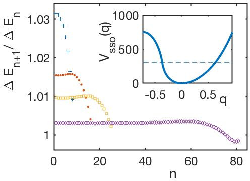
Figure 1: The scaled spacing $\frac{\Delta E_{n+1}}{\Delta E_{n}}$ of the eigenenergies of the SSO with varying excitation label $n$ for different values of the amplitude $\alpha$: From top to bottom we have $\alpha=10^{3},4\cdot 10^{3},10^{4},10^{5}$. Inset: the spatially and energetically shifted SSO potential well as given in the text for $\alpha=10^{3}$; the dashed line indicates the energy of the transition point.

We concentrate on the spectral properties below the transition point energy (see inset of Figure 1) which exhibits an intriguing scaling behaviour as we shall see below. Figure 1 shows the scaled spacing $\Delta R_{n}=\frac{\Delta E_{n+1}}{\Delta E_{n}}$, with $\Delta E_{n}=E_{n}-E_{n-1}$ being the difference of the eigenenergies of the $n-$th and the $n-1$st eigenstates, as a function of the degree of excitation for varying amplitude $\alpha$ of the SSO. First of all one observes that the values of the scaled spacing are always close to one, varying only by a few percent around one. For the case $\alpha=10^{3}$ with increasing degree of excitation the scaled spacing monotonically decreases ranging for low excitations in the vicinity of $1.03$ and for states close to the transition energy around $1.01$. For larger values of $\alpha$ a plateau emerges with approximately constant values for $\Delta R$ with $\Delta R=1.015,1.01,1.003$ for $\alpha=4\cdot 10^{3},10^{4},10^{5}$, respectively. This clearly indicates that there is a scaling property of the eigenvalue spectrum in the well of the SSO, and the scaling factor decreases towards the value one with increasing amplitude $\alpha$ of the SSO. The constancy of this scaling over a broad range of the spectrum is a remarkable property of the SSO.

A natural modification of the SSO potential is the skewed superexponential oscillator with the potential ${\cal{V}}_{sk}(q)=\alpha|\beta q|^{\gamma q}$. We remark that this skewed oscillator shows similar spectral properties as compared to the original SSO, and we therefore refrain from discussing it separately.

III The right-symmetrized SSO

A modification of the SSO, which introduces new properties into the spectrum, is obtained if we simply mirror the right half of the SSO potential well to the left and obtain in this way a reflection symmetry potential well. This is the so-called right-symmetrized SSO. Shifting it to zero energy and to the minimum position at the origin one obtains

$${\cal{V}}_{rso}(q)=\alpha\left(\left(q_{m}+|q|\right)^{\left(q_{m}+|q|\right)}-q_{m}^{q_{m}}\right)$$ (3)

where $q_{m}=e^{-1}$. The potential well of the right-symmetrized SSO is shown in the inset of Figure 2 for $\alpha=10^{3}$.

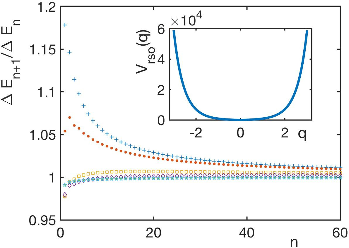
Figure 2: The scaled spacing $\Delta R_{n}=\frac{\Delta E_{n+1}}{\Delta E_{n}}$ of the eigenenergies of the right-symmetrized SSO with varying excitation label $n$ for different values of the amplitude $\alpha$: From top to bottom we have $\alpha=1,10,10^{3},10^{4},10^{6}$. Inset: the potential ${\cal{V}}_{rso}$ of the right-symmetrized SSO as given in the text for $\alpha=10^{3}$.

Figure 2 shows the scaled spacing $\Delta R_{n}$ of the eigenenergies of the right-symmetrized SSO as a function of the degree of excitation $n$ for varying amplitude $\alpha$ of the SSO. It shows a smooth approach with (in magnitude) monotonically decreasing slopes for the different values of $\alpha$ towards the asymptotics. For small values of $\alpha$, namely $\alpha=1,10$, $\Delta R_{n}$ is larger than the value one and decreases monotonically with increasing $n$ towards the values one. Opposite to this, for $\alpha=10^{6}$ $\Delta R_{n}$ is always less than one and increases monotonically towards one. For the intermediate cases $\alpha=10^{3},10^{4}$, $\Delta R_{n}$ increases with increasing $n$ from values smaller than one, then passes the threshold value of one and increases further. Subsequently (barely visible in Figure 2) it reaches a maximum (e.g. $n=18$ for $\alpha=10^{3}$) and decreases towards the value one with further increasing $n$. This clearly demonstrates that the right-symmetrized SSO and the SSO spectrum behave qualitatively different. This provides us with the promise of an even richer spectral structure when moving on to other superexponential trapping potentials. Indeed we will see this conjecture being verified below for other natural generalizations of the SSO.

IV The power law SSO

Let us now consider the right-symmetrized SSO with an extra power to possibly tune the spectral properties. The corresponding potential of this power law SSO reads as follows

$${\cal{V}}_{rpo}(q)=\alpha\left(\left(q_{m}+|q|\right)^{\left(\left(q_{m}+|q|\right)^{\beta}\right)}-q_{m}^{(q_{m}^{\beta})}\right)$$ (4)

where now $q_{m}=e^{-\frac{1}{\beta}}$ and we have two free parameters: the amplitude $\alpha$ and the exponent $\beta$ in the exponent. The inset of Figure 3 provides the potential ${\cal{V}}_{rpo}(q)$ for $\alpha=1$ with varying values of the parameter $\beta$. The increasingly steep confinement with an increasing value of $\beta$ is clearly visible. Figure 3 shows the scaled spacing $\Delta R_{n}$ of the eigenenergies of the power law SSO with varying excitation label $n$ for $\beta=0.5$ and for different values of the amplitude $\alpha$. The spectral behaviour is similar to the case of the right-symmetrized SSO discussed in the previous section, but now additionally we observe for low excitations that the monotonic behaviour of $\Delta R_{n}$ with increasing $n$ is violated: we encounter an increase versus decrease for the scaled spacing for consecutive values of $n$. This is much more pronounced for smaller values of the parameter $\beta$. Figure 4 addresses the case $\beta=0.25$ where in an alternating manner throughout the spectrum an increase is followed by a decrease of the scaled spacing $\Delta R_{n}$. In certain parts of the spectrum these oscillations even refer to values of $\Delta R_{n}$ above and below the value one.

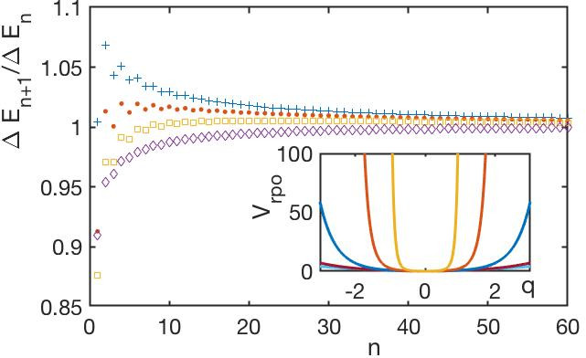
Figure 3: The scaled spacing $\Delta R_{n}=\frac{\Delta E_{n+1}}{\Delta E_{n}}$ of the eigenenergies of the power law SSO with varying excitation label $n$ for $\beta=0.5$ and different values of the amplitude $\alpha$: From top to bottom $\alpha=1,10,10^{2},10^{4}$. Inset: the potential ${\cal{V}}_{rpo}$ of the RPO as given in the text for $\alpha=1,\beta=0.25,0.5,1.0,2.0,4.0$ from bottom to top.

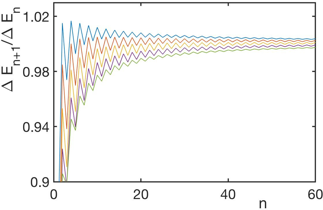
Figure 4: The scaled spacing $\Delta R_{n}=\frac{\Delta E_{n+1}}{\Delta E_{n}}$ of the eigenenergies of the RPO with varying excitation label $n$ for $\beta=0.25$ and different values of the amplitude $\alpha$: From top to bottom $\alpha=1,10,10^{2},10^{3},10^{4}$. To guide the eye the data points have been interconnected with straight lines.

V The oscillating power potential

Let us now allow for an oscillating periodic function in the exponent while we keep as a basis the magnitude of the coordinate $q$. We therefore introduce the oscillating power potentials (OPP) according to the following

$${\cal{V}}_{c}(\alpha,\beta,k;q)=|q|^{\alpha+\beta\cos(kq)}$$ (5)

$${\cal{V}}_{s}(\alpha,\beta,k;q)=|q|^{\alpha+\beta\sin(kq)}$$ (6)

These potentials are obviously very much different from a standard superposition of a harmonic confinement with a periodic lattice such as $V\propto q^{2}+\cos(q)$. Indeed, the OPP possess an oscillating power with amplitude $\beta$ and wavevector $k$ superimposed on a constant power $\alpha$. Figure 5(a) shows ${\cal{V}}_{c}$ for the parameter values $\alpha=0.3,\beta=0.05,k=1$. Apart from the existence of a central well with a cusp there is a series of decentered wells which become increasingly deeper with increasing distance from the outer well. The energies of the minima of those wells increase according to the constant power $|q|^{0.3}$ while moving away from the origin. These are a few relevant, but certainly not the only, properties which distinguish ${\cal{V}}_{c}$ from the above-mentioned case $V$: the OPP is a highly nonlinear potential via its oscillatory exponential appearance. Obviously, ${\cal{V}}_{c}$ is reflection symmetric around the origin, whereas ${\cal{V}}_{s}$ is asymmetric due to the odd character of the sine function in the exponent (see Figure 5(a)).

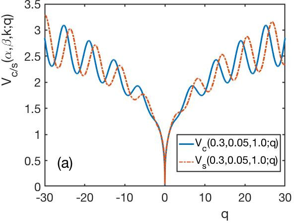
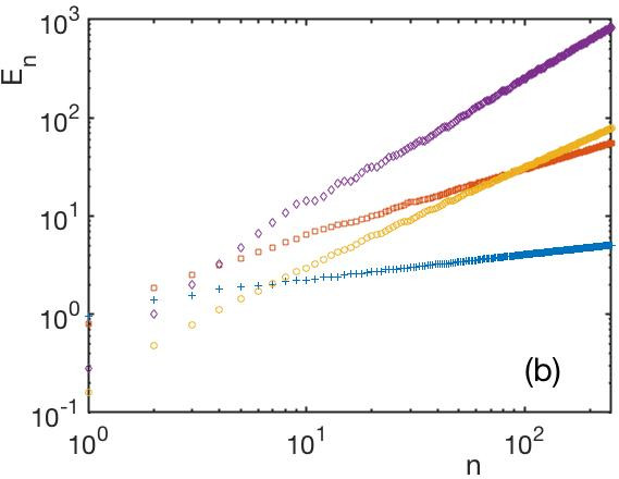
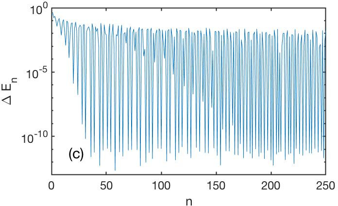
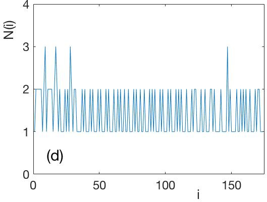
Figure 5: (a) The potentials ${\cal{V}}_{c}(\alpha,\beta,k;q)$ and correspondingly ${\cal{V}}_{s}(\alpha,\beta,k;q)$ (see text) for $\alpha=0.3,\beta=0.05,k=1$. (b) Log-log representation of the energy eigenvalues $E_{n}$ versus the excitation label $n$ for $\alpha=0.3,\beta=0.05,k=1,\gamma=1$ (crosses), $\alpha=1,\beta=0.05,k=1,\gamma=1$ (squares), $\alpha=2,\beta=0.1,k=3,\gamma=0.05$ (circles), $\alpha=4,\beta=1,k=2,\gamma=0.1$ (diamonds). (c) The spacing $\Delta E_{n}$ of the eigenenergies as a function of the excitation label $n$ for the potential ${\cal{V}}_{c}(\alpha,\beta,k;q)$ with $\alpha=0.3,\beta=0.05,k=1$ on a semilogarithmic scale. (d) The turning point characteristics $N(i)$ of the energy spacing dynamics (definition see text) shown in (c).

V.1 The sublinear OPP cosine case

Let us now focus on the spectral analysis of the OPP according to the solutions of the underlying SEQ. First we will discuss the eigenvalue spectrum and consequently the most important properties of the eigenstates. Figure 5(b) shows the energy eigenvalues $E_{n}$ versus the excitation label $n$ for the $250$ energetically lowest eigenstates in a double logarithmic representation for the case $\alpha=0.3,\beta=0.05,k=1$ and for $\gamma=1$ where $\gamma$ is an additional prefactor (amplitude) of the overall potential. As expected, according to the constant power in the exponent, the mean behaviour of the spectrum follows a power law according to $E\propto n^{0.26}$. Figure 5(c) shows the spacing $\Delta E_{n}$ with varying degree of excitation $n$ on a semilogarithmic scale. First of all one observes an overall decrease of the spacings with increasing $n$. Beyond this, the eyecatching feature is the highly oscillatory character over many orders of magnitude of this spacing ’dynamics’. Starting from the ground state energy and increasing the value of $n$ we observe a series of turning points in the spacing dynamics (see Figure 5(c)) which belong to increasingly lower values of the spacings, i.e. a series of near degeneracies of two neighboring energy levels occur in the spectrum. In between these near degeneracies the spacing returns to values of the order of $10^{-2}$. For $n>20$ those near degenerate levels involve spacings smaller than $10^{-10}$ and cannot be completely resolved within our numerical approach. For $n>60$ a second series of increasingly narrower near degeneracies emerges with further increasing degree of excitation $n$. As a result the ’density’ of near degeneracies in the spectrum is enhanced.

To gain more insights into the oscillatory dynamics of the energy spacing with increasing degree of excitation we employ a turning point analysis. Let us define the turning point characteristics $N(i)$ as the number of level spacings between two turning points of the level spacing dynamics. The index $i$ represents just the increasing natural numbers counting these level spacings between turning points. A value of one means that two turning points follow upon each other without the presence of a second spacing whereas a value of two indicates the presence of a second spacing before the next turning point occurs. In Figure 5(d) we observe that the values one and two dominate $N(i)$: the dynamics shows trains of alternating values one and two occasionally interrupted by intervals showing two consecutive values one. Very rarely high peaks with the value three occur, i.e. the spacing increases/decreases consecutively among four eigenenergies following upon each other. This energy spacing analysis provides a comprehensive view on the level dynamics and we will use it in the following to characterize the spectral properties of the different superexponential potentials.

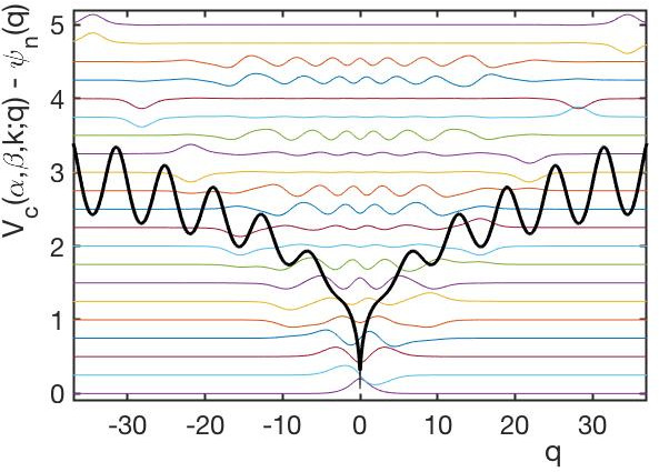
Figure 6: The potential ${\cal{V}}_{c}(\alpha,\beta,k;q)$ for $\alpha=0.3,\beta=0.05,k=1$ together with the energetically lowest $21$ eigenstates (shown are the non-normalized probability amplitudes). Note that the vertical arrangement of the eigenstates is not associated with the detailed energetical position of these eigenstates.

Let us now inspect the eigenstates of the sublinear OPP cosine case. This will provide us with an understanding of the origin of the near degeneracies observed above. Figure 6 shows the potential ${\cal{V}}_{c}(\alpha,\beta,k;q)$ for $\alpha=0.3,\beta=0.05,k=1$ together with the energetically lowest $21$ eigenstates. Starting from the ground state the energetically lowest four states are localized in the central well of the OPP. Thereafter, with further increasing degree of excitation, more and more outer wells are covered with increasing energy. A closer inspection reveals that there is two classes of states. The first class is the expected class of delocalized eigenstates covering a certain range of the OPP. Interspersed into these delocalized states we encounter localized states that carry a significant probability amplitude only in some outer wells. They occur in pairs with even and odd parity. In Figure 6 these are, e.g. the pairs of the $(9,10)-$th states, or, showing an even stronger localization, the $(13,14)-$th, $(16,17)-$ or $(20,21)-$st eigenstates. The localization happens in (or above) a certain outer well and becomes increasingly more pronounced with increasing degree of excitation of the considered eigenstate. In essence, these localized states appear to consist, to some degree of approximation, of two single humped probability amplitudes localized at the positions of certain outer wells whose depths increases with increasing distance from the central well and therefore the degree of localization becomes increasingly more pronounced.

V.2 The sublinear OPP sine case

Let us now explore the spectral properties of the OPP ${\cal{V}}_{s}(\alpha,\beta,k;q)$. It has no inversion symmetry w.r.t. the origin and therefore the eigenstates are not parity symmetric. In other words, the inversion symmetry ${\cal{V}}_{c}(\alpha,\beta,k;q)={\cal{V}}_{c}(\alpha,\beta,k;-q)$ is maximally broken for ${\cal{V}}_{s}$, see also Figure 5(a) for the case $\alpha=0.3,\beta=0.05,k=1$. At equal distance from the origin the left and right outer wells are (approximately) shifted by a phase of $\frac{\pi}{2}$ i.e. if one encounters a maximum on the left branch of the OPP the reflection symmetric position to the right represents a minimum and vice versa.

The smooth mean part of the behaviour of the eigenenergies with increasing degree of excitation is for the OPP ${\cal{V}}_{s}$ the same as the one for ${\cal{V}}_{c}$, i.e. it obeys a power law $E\propto n^{0.26}$. Major differences however are revealed when focusing on the fluctuations or the level spacing dynamics.

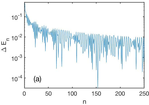
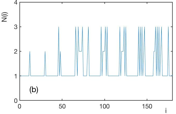
Figure 7: (a) The spacing $\Delta E_{n}$ of the eigenenergies as a function of the excitation label $n$ for the potential ${\cal{V}}_{s}(\alpha,\beta,k;q)$ for $\alpha=0.3,\beta=0.05,k=1$ on a semilogarithmic scale and (b) the turning point characteristics $N(i)$ of the energy spacing dynamics (definition see text) shown in (a).

Figure 7(a) shows the spacing $\Delta E_{n}$ of the eigenenergies as a function of the excitation label $n$ for the potential ${\cal{V}}_{s}(\alpha,\beta,k;q)$ for $\alpha=0.3,\beta=0.05,k=1$ on a semilogarithmic scale. Obviously a very rich energy spacing dynamics can be observed. Apart from an expected overall decay of the spacing we observe a beating behaviour and, within these beats i.e. on the shortest scale, alternating spacings of increasing and decreasing values between nearest neighbor spacings or next to nearest neighbor spacings. The beats dissolve respectively overlap for larger values of the excitation $n$. While the spectrum of the OPP ${\cal{V}}_{c}(\alpha,\beta,k;q)$ (see subsection V.1) contains a large number or series of near degeneracies this is now not the case for the spectrum of the OPP ${\cal{V}}_{c}(\alpha,\beta,k;q)$: there is only a very limited range of values for the spacings, typically $10^{-4}<\Delta E_{n}<10^{-1}$, i.e. the near degeneracies of ${\cal{V}}_{c}$ are lifted due to the broken parity symmetry. Figure 7(b) shows the turning point characteristics $N(i)$ of the energy spacing dynamics. Compared to Figure 5(d), which shows $N(i)$ for the OPP ${\cal{V}}_{c}$, we encounter now many subsequent events with a single spacing. The reader should be reminded that the value one for $N(i)$ corresponds to a single spacing between turning points of the energy level dynamics, i.e. an alternating increase and decrease of the spacing. In between these extended intervals of value one, $N(i)$ shows finite series of peaks with values two and three arranged in a repeating manner.

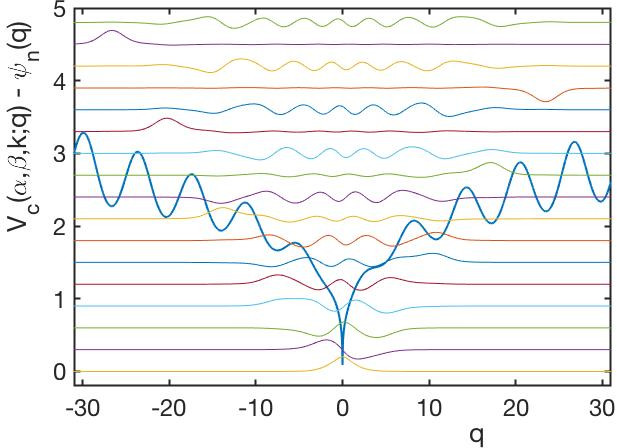
Figure 8: The potential ${\cal{V}}_{s}(\alpha,\beta,k;q)$ for $\alpha=0.3,\beta=0.05,k=1$ together with the energetically lowest $17$ eigenstates (shown are the non-normalized probability amplitudes).

Figure 8 shows the potential ${\cal{V}}_{s}(\alpha,\beta,k;q)$ for $\alpha=0.3,\beta=0.05,k=1$ together with the probability amplitude of the energetically lowest $17$ eigenstates. As for the case of ${\cal{V}}_{c}$ (see subsection V.1) there are localized states interspersed between delocalized states. Now, however, due to the missing parity symmetry of the eigenstates there is either right or left localized states. In Figure 8 these are the $10,12,14,16-$th eigenstate which can be, according to their localization, assigned to the corresponding outer potential wells on either the left or the right half of the OPP.

V.3 The sublinear OPP case with arbitrary phase

Having explored the spectral properties of ${\cal{V}}_{c}$ and ${\cal{V}}_{s}$ including the presence and lifting of near degeneracies as well as the localization and delocalization of the underlying eigenstates, our focus in this brief subsection is to mediate between the two cases. To this end we investigate the spectrum of the potential

$${\cal{V}}_{p}(\alpha,\beta,k,\phi;q)=|q|^{\alpha+\beta\sin(q+\phi)}$$ (7)

which coincides with ${\cal{V}}_{c}$ and ${\cal{V}}_{s}$ for $\phi=\frac{\pi}{2}$ and $\phi=0$, respectively. We again focus on the parameter values $\alpha=0.3,\beta=0.05,k=1$ and vary $\phi$ continuously from $0$ to $2\pi$. This way we expect to see the crossover between the spectral properties of the limiting cases considered above. Figure 9 shows the eigenvalue spectrum as a function of the phase $\phi$ for ${\cal{V}}_{p}$ for the energetically lowest 21 eigenstates. It can be seen that near degeneracies and avoided crossings, which become increasingly narrow with increasing degree of excitation, occur at $\phi=\frac{\pi}{2},\frac{3\pi}{2}$ and are lifted once moving off from these configurations. At $\phi=0,\pi,2\pi$ these close encounters of the energy levels are not present throughout the spectrum. The doublet formation and splitting can therefore be controlled by varying the phase $\phi$. This is somehow reminescent of the splitting of the single particle eigenstates in a double well Schmelcher1 ; Oberthaler which determines the frequency of the Rabi oscillations when considering the dynamics following a wave packet in a single well. In our superexponential setup the situation is different in the following sense. With increasing degree of excitation or increasing energy, the eigenstates of the doublets refer, in terms of their localization, to different spatially well-separated individual outer wells attached to the overall confining potential well. As a consequence the resulting quantum dynamics of a wave packet, being left or right localized due to a superposition of the two states of the doublet, would provide a quantum state transfer between remote pairs of individual wells attached to the confining walls of the overall potential (see also remarks in the conclusions). It should also be noted that the shape of those individual wells and consequently also of the corresponding localized wave packets differ significantly from the one of the individual wells commonly encountered in optical lattices and correspondingly from their Wannier states.

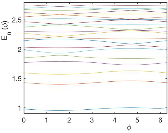
Figure 9: The eigenvalue spectrum as a function of the phase $\phi$ (in arc measure) for the potential ${\cal{V}}_{p}=|q|^{0.3+0.05\sin(q+\phi)}$ for the energetically lowest 21 eigenstates.

V.4 The linear OPP cosine case

In this subsection we explore the case $\alpha=1$ i.e. the case of a linear behaviour due to the constant part of the exponent combined with an oscillating cosine in the exponent again with an amplitude $\beta=0.05$. The corresponding potential ${\cal{V}}_{c}(\alpha,\beta,k;q)$ is shown for $k=1$ in Figure 10(a). Figure 5(b) shows the mean power law dependence of the eigenenergies with increasing excitation label for which $E\propto n^{0.72}$ holds. Figure 10(b) provides a semi-logarithmic representation of the corresponding spacing $\Delta E_{n}$ of the energy eigenvalues versus the excitation label $n$. First of all we observe a very ’slow’ overall decrease of the spacing with increasing degree of excitation $n$. More important, however, is the occurence of near degeneracies which are again interspersed into the spectrum of spacings whose predominant range of values is $10^{-2}<\Delta E_{n}<1$.

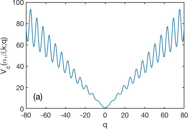
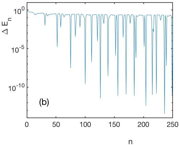
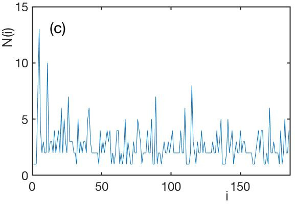
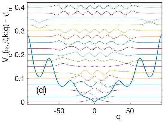
Figure 10: (a) The potential ${\cal{V}}_{c}(\alpha,\beta,k;q)$ (see text) for $\alpha=1.0,\beta=0.05,k=1$. (b) Semi-logarithmic representation of the spacing of the energy eigenvalues $E_{n}$ versus the excitation label $n$ for the potential shown in (a). (c) The corresponding turning point characteristics $N(i)$ of the energy spacing dynamics (definition see text) shown in (b). (d) The potential $\gamma{\cal{V}}_{c}(\alpha,\beta,k;q)$ for $\alpha=1.0,\beta=0.09,k=0.2,\gamma=0.002$ together with the energetically lowest $17$ eigenstates (shown are the non-normalized probability amplitudes).

Figure 10(c) shows the corresponding turning point characteristics $N(i)$ of the energy spacing dynamics. Opposite to the above considered cases of superexponential potentials a direct alternation in the spectrum corresponding to a value of one, is now encountered very rarely. Instead, there is now a range of values up to $13$ which is covered in the considered window of the eigenenergy spectrum. Overall $N(i)$ looks rather irregular while still certain patterns or bursts of spacing sequences are recognizable. Figure 10(d) presents the potential $\gamma{\cal{V}}_{c}(\alpha,\beta,k;q)$ for $\alpha=1.0,\beta=0.09,k=0.2,\gamma=0.002$ and its energetically lowest $17$ eigenstates. Delocalized states and states localized in outer wells, being parity symmetric or antisymmetric, can be identified as for the above-discussed cases of the OPP.

V.5 The quadratic and quartic OPP cosine case

Let us briefly study the spectral properties for the quadratic and quartic case, i.e. for $\alpha=2$ respectively $\alpha=4$. In Figure 11(a) the potential $\gamma\cdot{\cal{V}}_{c}(\alpha,\beta,k;q)$ for $\alpha=2.0,\beta=0.1,k=3.0,\gamma=0.05$ is illustrated. The deepening of the potential wells attached to the (average) potential walls, which represent a harmonic oscillator, are clearly visible. We therefore expect also for this reflection symmetric case the appearance of near degenerate doublets in the energy spectrum. Indeed inspecting the dynamics of the spacing of the energy eigenvalues shown in Figure 11(b) one observes with increasing degree of excitation $n$ the emergence of near degeneracies. More specifically, there is two such series of near degeneracies, the first one starting at approximately $n=50$ and second one arising close to $n=120$ (the onset of a third series is visible too for $n>200$). The mean behaviour of $E_{n}$, as expected, follows a power law $E_{n}\propto n$ (see Figure 5(b)) and therefore the spacing fluctuates around a constant value (see Figure 11(b)). The corresponding turning point characteristics $N(i)$ is illustrated in Figure 11(c). Many equally spaced events with values $N(i)>2$ can be observed for higher excitations, whereas for lower excitations more rapid oscillations also for $N(i)>2$ are observed. $N(i)$ bears quite some similarities but also major differences to the linear case discussed in subsection V.4, whereas it is overall distinctly different from the sublinear case discussed in subsections V,V.1,V.2,V.3.

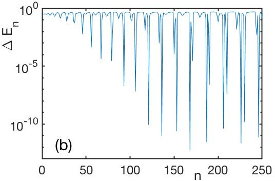
Figure 11: (a) The potential $\gamma{\cal{V}}_{c}(\alpha,\beta,k;q)$ for $\alpha=2.0,\beta=0.1,k=3.0,\gamma=0.05$. (b) Semi-logarithmic representation of the spacing of the energy eigenvalues $E_{n}$ versus the excitation label $n$ for the potential shown in (a). (c) The corresponding turning point characteristics $N(i)$ of the energy spacing dynamics (definition see text) shown in (b).

Figure 12 shows, as a final case, the potential $\gamma{\cal{V}}_{c}(\alpha,\beta,k;q)$ for $\alpha=4.0,\beta=1.0,k=2.0,\gamma=0.1$ where the first few ’side-pockets’ attached to the steep walls of the overall $q^{4}$-confinement are clearly visible. Also shown are the localized eigenstates in this potential which correspond to the $10-11th,15-16th,20-21st,34-35th$ and $43-44th$ pairs of eigenstates with odd and even parity correspondingly. For the higher excited states the localization is almost perfect, as can be seen in Figure 12.

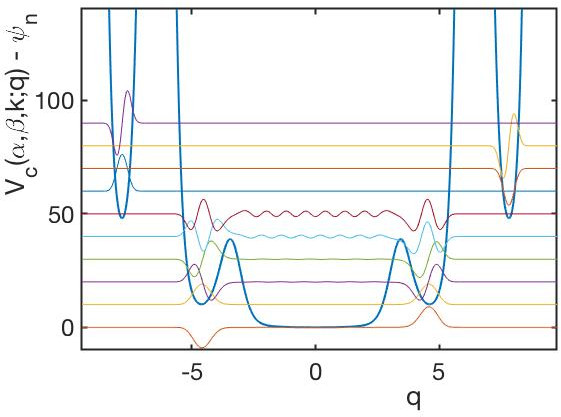
Figure 12: The potential $\gamma{\cal{V}}_{c}(\alpha,\beta,k;q)$ for $\alpha=4.0,\beta=1.0,k=2.0,\gamma=0.1$ together with the localized states corresponding to the $10-11th,15-16th,20-21st,34-35th,43-44th$ pairs of eigenstates (shown are the non-normalized probability amplitudes).

VI Conclusions

The few existing investigations on superexponential model systems Schmelcher2 ; Schmelcher3 ; Schmelcher4 ; Schmelcher5 have demonstrated that they exhibit a variety of peculiar phenomena and properties. Motivated by this and in particular by the importance of the geometry of trapping potentials in a diversity of research problems, encompassing optical tweezers for soft matter manipulation and processing of atomic degenerate quantum gases, we have performed in this work a first step towards the exploration of the spectral properties of confining superexponential potentials.

The original self-interacting superexponential oscillator (SSO) has been shown in ref.Schmelcher5 to exhibit a crossover of its eigenvalue spectrum from a scaling behaviour below its transition point to irregular oscillations above the transition energy. Building on that we started here by analyzing the spectrum of the SSO with varying amplitude. This way we have illuminated the emergence of the scaling behaviour of the eigenvalues with increasing amplitude. In a second step we modified the SSO in several ways in order to demonstrate the variations of the spectrum. For the symmetrized SSO a smooth approach of the scaled spacing $\frac{\Delta E_{n+1}}{\Delta E_{n}}$ with increasing degree of excitation is observed towards the value one, either from above or below one, depending on its amplitude. For low excitations a crossover of the scaled spacing from increasing to decreasing behaviour and from values below one to above one is observed. Augmented by a power law in the exponent we have analyzed the so-called power law SSO: here the scaled spacing shows an alternating increasing and decreasing behaviour between neighboring energy spacings of the energy levels. The mean behaviour is similar to the one obtained for the symmetrized SSO.

In the second part of our investigations we have explored potentials with a spatially oscillating power (OPP) in combination with a constant part. These potentials exhibit a central well and an infinite series of left and right located side wells whose depths increases with increasing distance from the central well. We have analyzed the eigenenergy spacing dynamics and revealed several interesting properties depending on the constant part of the power and the phase of the oscillating power. The sublinear, linear as well as quadratic and quartic case have been considered. Depending on the phase these potentials show a reflection symmetry or not. In the presence of the reflection symmetry a series of energetically near degenerate doublets of eigenstates emerges with an increasingly smaller splitting with increasing degree of excitation. While the remainder of the eigenstates are delocalized these doublet states are localized in a left right pair of outer wells. Breaking the reflection symmetry separates the states of this doublet in energy, i.e. removes the near degeneracy, and introduces an exclusive left or right localization.

Based on the above diverse spectral properties of superexponential potentials, there is several possible future directions of investigation and potential applications. Preparing as an initial state a superposition state of the parity symmetric partner eigenstates of a doublet the resulting quantum dynamics would be an oscillation between right and left localized wave packets, i.e. a remote transfer or delivery of particles, or, in other words, Rabi oscillations between remotely placed potential wells. One might then conjecture that superpositioning more than just one doublet, leads to a ’collective’ type of Rabi oscillations between several occupied outer wells involving different frequencies, which is an intriguing feature of the OPP. Another relevant question is how interactions would modify or enrich this picture - meaning both the spectral structure as well as the resulting quantum dynamics. Related to this general direction of investigation would be the question of the emergence of entanglement in the OPP.

Changing the phase of the OPP in time may yield a delivery of particles, even particle by particle, or atom by atom, to the central well. The OPP could therefore potentially be used as a rechargeable tweezer where the ’focus’ atom to be processed is in the central well and, once this atom is gone, the central well can be reloaded by changing the phase of the OPP and transfering atoms from the side wells to the central well. A very promising physical platform to realize this would be ultracold atoms which can be prepared, processed and detected on a single atom level Ott . The OPP might be created by one of the extremely powerful techniques of light beam engineering. Traps with almost arbitrary geometry can be designed nowadays Grimm including optical tweezer arrangements Kuhn using spatial light modulators or so-called painted dynamic potentials which can create by a rapidly moving laser beam time-averaged optical dipole potentials of arbitrary shape Boshier .

VII Acknowledgments

The author acknowledges K. Keiler for a careful reading of the manuscript.

References

- (1) Low temperatures and cold molecules, Imperial College Press, edited by Ian W M Smith (2008)
- (2) Cold molecules: theory, experiment and applications, CRC Press, edited by R.V. Krems, W.C. Stwalley and B. Friedrich (2009).
- (3) Handbook of Photonics for Biomedical Engineering, Springer Reference, edited by A.H.P. Ho, D. Kim, M.G. Somekh (2017).
- (4) C.J. Pethick and H. Smith, Bose-Einstein condensation in dilute gases, 2nd edition, Cambridge University Press (2008).
- (5) H.J. Metcalf and P. van der Straten, Laser cooling and trapping, Springer (2013).
- (6) R. Grimm, M. Weidemüller and Y.B. Ovchinnikov, Adv.At.Mol.Opt.Phys. 42, 95 (2000).
- (7) C. Chin, R. Grimm, P. Julienne, and E. Tiesinga, Rev.Mod.Phys. 82, 1225 (2010).
- (8) D.J. Frantzeskakis, J.Phys.A 43, 213001 (2010).
- (9) M. Bohlen, L. Sobirey, N. Luick, H. Biss, T. Enss, T. Lompe, and H. Moritz, Phys.Rev.Lett. 124, 240403 (2020).
- (10) S. Zöllner, H.D. Meyer and P. Schmelcher, Phys.Rev.Lett. 100, 040401 (2008).
- (11) M. Albiez, R. Gati, J. Fölling, S. Hunsmann, M. Cristiani, and M.K. Oberthaler, Phys.Rev.Lett. 95, 010402 (2005).
- (12) I. Bloch, J. Dalibard, W. Zwerger, Rev.Mod.Phys. 80, 885 (2008).
- (13) M. Greiner, O. Mandel, T. Esslinger, T.W. Hänsch and I. Bloch, Nature 415, 39 (2002).
- (14) P. Schmelcher, Commun.Nonl.Sci.Num.Sim. 95, 105599 (2021).
- (15) P. Schmelcher, acc.f.publ. Comm.Nonl.Sci.Num.Sim., arXiv:2011.13672.
- (16) P. Schmelcher, J.Phys. A 53, 075701 (2020).
- (17) P. Schmelcher, J.Phys. A 53, 305301 (2020).
- (18) G.C. Groenenboom and H.M. Buck, J.Chem.Phys. 92, 4374 (1990).
- (19) H. Ott, Rep.Prog.Phys. 79, 054401 (2016).
- (20) C.Muldoon, L. Brandt, J. Dong, D. Stuart, E. Brainis, M. Himsworth, and A. Kuhn, New J. Phys. 14, 073051 (2012).
- (21) K. Henderson, C. Ryu, C. MacCormick and M.G. Boshier, New.J.Phys. 11, 043030 (2009).