Conformalized Survival Analysis

Abstract

Existing survival analysis techniques heavily rely on strong modelling assumptions and are, therefore, prone to model misspecification errors. In this paper, we develop an inferential method based on ideas from conformal prediction, which can wrap around any survival prediction algorithm to produce calibrated, covariate-dependent lower predictive bounds on survival times. In the Type I right-censoring setting, when the censoring times are completely exogenous, the lower predictive bounds have guaranteed coverage in finite samples without any assumptions other than that of operating on independent and identically distributed data points. Under a more general conditionally independent censoring assumption, the bounds satisfy a doubly robust property which states the following: marginal coverage is approximately guaranteed if either the censoring mechanism or the conditional survival function is estimated well. Further, we demonstrate that the lower predictive bounds remain valid and informative for other types of censoring. The validity and efficiency of our procedure are demonstrated on synthetic data and real COVID-19 data from the UK Biobank.

1 Introduction

The COVID-19 pandemic has placed extraordinary demands on health systems (e.g., Ranney et al., 2020). In turn, these demands create an unavoidable need for medical resource allocation and, in response, several groups of researchers have communicated clinical ethics recommendations (e.g., Emanuel et al., 2020; Vergano et al., 2020). By and large, these recommendations require a reliable individual risk assessment for patients who test positive; see Table 2 of Emanuel et al. (2020). Clearly, one risk measure of interest might be the survival time, the time lapse between the confirmation of COVID-19 and an event such as death or reaching a critical state, should this ever occur.

1.1 Survival analysis

Survival times are not always observed due to censoring (Leung et al., 1997). A main goal of survival analysis is to infer the survival function—the probability that a patient will survive beyond any specified time—from censored data. The Kaplan-Meier curve (Kaplan and Meier, 1958) produces such an inference when the population under study is a group of patients with certain characteristics. On the positive side, the Kaplan-Meier curve does not make any assumption on the distribution of survival times. On the negative side, it can only be applied to a handful of subpopulations because it requires sufficiently many events in each subgroup (Kalbfleisch and Prentice, 2011). More often than not, the scientist has available multiple categorical and continuous covariates, and it thus becomes of interest to understand heterogeneity by studying the conditional survival function; that is, the dependence on the available factors. In the conditional setting, however, distribution-free inference for the conditional survival function gets to be challenging. Standard approaches make parametric or nonparametric assumptions about the distribution of the covariates and that of the survival times conditional on covariate values. A well-known example is of course the celebrated Cox model which posits a proportional hazards model in which an unspecified nonparametric base line is modified via a parametric model describing how the hazard varies in response to explanatory covariates (Cox, 1972; Breslow, 1975). Other popular models, such as accelerated failure time (AFT) (Cox, 1972; Wei, 1992) and proportional odds models (Murphy et al., 1997; Harrell Jr, 2015), also combine nonparametric and parametric model specifications.

As medical technologies produce ever larger and more complex clinical datasets, we have witnessed a rapid development of machine learning methods adapted to high-dimensional and heterogeneous survival data (e.g., Verweij and Van Houwelingen, 1993; Faraggi and Simon, 1995; Tibshirani, 1997; Gui and Li, 2005; Hothorn et al., 2006; Zhang and Lu, 2007; Ishwaran et al., 2008; Witten and Tibshirani, 2010; Goeman, 2010; Simon et al., 2011; Katzman et al., 2016; Lao et al., 2017; Wang et al., 2019; Li and Bradic, 2020). An appealing feature of these methods is that they typically do not make modeling assumptions. To quote from Efron (2020): “ Neither surface nor noise is required as input to randomForest, gbm, or their kin.” The downside is that it is often challenging to quantify the uncertainty for these methods. To be sure, blind application of off-the-shelf uncertainty quantification tools, such as the bootstrap (Efron, 1979; Efron and Tibshirani, 1994), can yield unreliable results since their validity 1) rests on implicit modeling assumptions, and 2) holds only asymptotically (e.g., Lei and Candès, 2021; Ratkovic and Tingley, 2021).

1.2 Prediction intervals

For decision-making in sensitive and uncertain environments—think of the COVID-19 pandemic—it is preferable to produce prediction intervals for the uncensored survival time with guaranteed coverage rather than point predictions. In this regard, the use of $(1-\alpha)$ prediction intervals is an effective way of summarizing what can be learned from the available data; wide intervals reveal a lack of knowledge and keep overconfidence at arm’s length. Here and below, an interval is said to be a $(1-\alpha)$ prediction interval if it has the property that it contains the true label, here, the survival time, at least $100(1-\alpha)$% of the time (a formal definition is in Section 2). Prediction intervals have been widely studied in statistics (e.g., Wilks, 1941; Wald, 1943; Aitchison and Dunsmore, 1980; Stine, 1985; Geisser, 1993; Vovk et al., 2005; Krishnamoorthy and Mathew, 2009) and much research has been concerned with the construction of covariate-dependent intervals.

Of special interest is the subject of conformal inference, a generic procedure that can be used in conjunction with sophisticated machine learning prediction algorithms to produce prediction intervals with valid marginal coverage without making any distributional assumption whatsoever (e.g., Saunders et al., 1999; Vovk, 2002; Vovk et al., 2005; Lei and Wasserman, 2014; Tibshirani et al., 2019). While coverage is only guaranteed in a marginal sense, it has been theoretically proved and empirically observed that some conformal prediction methods can also achieve near conditional coverage—that is, coverage assuming a fixed value of the covariates—when some key parameters of the underlying conditional distribution can be estimated reasonably well (e.g., Sesia and Candès, 2020; Lei and Candès, 2021).

1.3 Our contribution

Standard conformal inference requires fully observed outcomes and is not directly applicable to samples with censored outcomes. In this paper, we extend conformal inference to handle right-censored outcomes in the setting of Type-I censoring (e.g., Leung et al., 1997). This setting assumes that the censoring time is observed for every unit while the outcome is only observed for uncensored units. In particular, we generate a covariate-dependent lower prediction bound (LPB) on the uncensored survival time, which can be regarded as a one-sided $(1-\alpha)$-prediction interval. As we just argued, the LPB is a conservative assessment of the survival time, which is particularly desirable for high-stakes decision-making. A low LPB value suggests either a high risk for the patient, or a high degree of uncertainty for similar patients due to data scarcity. Either way, the signal to a decision-maker is that the patient deserves some attention.

Under the completely independent censoring assumption defined below, which states that the censoring time is independent of both the outcome and covariates, our LPB provably yields a $(1-\alpha)$ prediction interval. This property holds in finite samples without any assumption other than that of operating on i.i.d. samples. Under the more general conditionally independent censoring assumption introduced later, our LPB satisfies a doubly robust property which states the following: marginal coverage is approximately guaranteed if either the censoring mechanism or the conditional survival function is estimated well. In the latter case, the LPB even has approximately guaranteed conditional coverage.

Readers familiar with conformal inference would notice that the above guarantees can be achieved by simply applying conformal inference to the censored outcomes, i.e., by constructing an LPB on the censored outcome treated as the response. This unsophisticated approach is conservative. Instead, we will see how to provide tighter bounds and sharper inference by applying conformal inference on a subpopulation with large censoring times; that is, on which censored outcomes are closer to actual outcomes. To achieve this, we shall see how to carefully combine the selection of a subpopulation with ideas from weighted conformal inference (Tibshirani et al., 2019).

Lastly, while we focus on clinical examples, it will be clear from our exposition that our methods can be applied to other time-to-event outcomes in a variety of other disciplines, such as industrial life testing (Bain, 2017), sociology (Allison, 1984), and economics (Powell, 1986; Hong and Tamer, 2003; Sant’Anna, 2016).

2 Prediction intervals for survival times

2.1 Problem setup

Let $X_{i},C_{i},T_{i}$, $i=1,\ldots,n$, be respectively the vector of covariates, the censoring time, and the survival time of the $i$-th unit/patient. Throughout the paper, we assume that $(X_{i},C_{i},T_{i})$ are i.i.d. copies of the random vector $(X,C,T)$. We consider the Type I right-censoring setting, where the observables for the $i$-th unit include $X_{i},C_{i}$, and the censored survival time ${\widetilde{T}}_{i}$, defined as the minimum of the survival and censoring time:

$${\widetilde{T}}_{i}=\min(T_{i},C_{i}).$$

For instance, if $T_{i}$ measures the time lapse between the admission into the hospital and death, and $C_{i}$ measures the time lapse between the admission into the hospital and the day data analysis is conducted, then ${\widetilde{T}}_{i}=T_{i}$ if the $i$-th patient died before the day of data analysis and ${\widetilde{T}}_{i}=C_{i}$ if she survives beyond that day.

The censoring time $C$ partially masks information from the inferential target $T$. As discussed by Leung et al. (1997), it is necessary to impose constraints on the dependence structure between $T$ and $C$ to enable meaningful inference. In particular, we make the following conditionally independent censoring assumption (e.g., Kalbfleisch and Prentice, 2011):

Assumption 1 (conditionally independent censoring)

$$T~{}\rotatebox[origin={c}]{90.0}{$\models$}~{}C\mid X.$$ (1)

This assumes away any unmeasured confounder affecting both the survival and censoring time; please see immediately below for an example. In some cases, we also consider the completely independent censoring assumption, which is stronger in the sense that it implies the former:

Assumption 2 (completely independent censoring)

$$(T,X)~{}\rotatebox[origin={c}]{90.0}{$\models$}~{}C.$$ (2)

For instance, in a randomized clinical trial, the end-of-study censoring time $C$ is defined as the time lapse between the recruitment and the end of the study. For single-site trials, $C$ is often modelled as a draw from an exogenous stochastic process (e.g., Carter, 2004; Gajewski et al., 2008) and thus obeys (2). For multicentral trials, $C$ is often assumed to depend on the site location only (e.g., Carter et al., 2005; Anisimov and Fedorov, 2007; Barnard et al., 2010), and thus (1) holds as soon as the vector of covariates includes the site of the trial. For an observational study such as the COVID-19 example discussed later in Section 5, additional covariates would be included to make the conditionally independent censoring assumption plausible.

Although (1) is a strong assumption, it is a widely used starting point to study survival analysis methods (Kalbfleisch and Prentice, 2011). We leave the investigation of informative censoring (e.g., Lagakos, 1979; Wu and Carroll, 1988; Scharfstein and Robins, 2002) to future research. Additionally, whereas the setting of Type I censoring appears to be restrictive, we will show in Section 6.1 that an LPB in this setting can still be informative for other censoring types.

2.2 Naive lower prediction bounds

Our ultimate goal is to generate a covariate-dependent LPB as a conservative assessment of the uncensored survival time $T$. Denote by $\hat{L}(\cdot)$ a generic LPB estimated from the observed data $(X_{i},C_{i},{\widetilde{T}}_{i})_{i=1}^{n}$. We say an LPB is calibrated if it satisfies the following coverage criterion:

$$\mathbb{P}\big{(}T\geq\hat{L}(X)\big{)}\geq 1-\alpha,$$ (3)

where $\alpha$ is a pre-specified level (e.g., $0.1$), and the probability is computed over both $\hat{L}(\cdot)$ and a future unit $(X,C,T)$ that is independent of $(X_{i},C_{i},T_{i})_{i=1}^{n}$.

Since ${\widetilde{T}}\leq T$, any calibrated LPB on the censored survival time ${\widetilde{T}}$ is also a calibrated LPB on the uncensored survival time $T$. Consequently, a naive approach is to discard the censoring time $C_{i}$’s and construct an LPB on ${\widetilde{T}}$ directly. Since the samples $(X_{i},{\widetilde{T}}_{i})$ are i.i.d., a distribution-free calibrated LPB on ${\widetilde{T}}$ can be obtained via standard techniques from conformal inference (e.g., Vovk et al., 2005; Lei et al., 2018; Romano et al., 2019b). Our first result is somewhat negative: indeed, it states that all distribution-free calibrated LPBs on $T$ must be LPBs on ${\widetilde{T}}$.

Theorem 1

Take $X\in\mathbb{R}^{p}$ and $C\geq 0$, $T\geq 0$. Assume that $\hat{L}(\cdot)$ is a calibrated LPB on $T$ for all joint distributions of $(X,C,T)$ obeying the conditionally independent censoring assumption with $X$ being continuous and $(T,C)$ being continuous or discrete. Then for any such distribution,

$$\mathbb{P}({\widetilde{T}}\geq\hat{L}(X))\geq 1-\alpha.$$

Our proof can be extended to include the case where either $C$ or $T$ or both are mixtures of discrete and continuous distributions but we do not consider such extensions here. An LPB constructed by taking ${\widetilde{T}}$ as the response may be calibrated but also overly conservative because of the censoring mechanism. To see this, note that the oracle LPB on ${\widetilde{T}}$ is, by definition, the $\alpha$-th conditional quantile of ${\widetilde{T}}\mid X$, denoted by $\tilde{q}_{\alpha}(X)$. Similarly, let $q_{\alpha}(X)$ be the oracle LPB on $T$. Under the conditionally independent censoring assumption,

$$\mathbb{P}(T\geq q_{\alpha}(x)\mid X=x)=1-\alpha =\mathbb{P}({\widetilde{T}}\geq\tilde{q}_{\alpha}(x)\mid X=x)$$

$$=\mathbb{P}(T\geq\tilde{q}_{\alpha}(x)\mid X=x)\mathbb{P}(C\geq\tilde{q}_{\alpha}(x)\mid X=x).$$ (4)

If the censoring times are small, the gap between $\tilde{q}_{\alpha}(x)$ and $q_{\alpha}(x)$ can be large. For illustration, assume that $X,C$, and $T$ are mutually independent, and $T\sim\mathrm{Exp}(1),C\sim\mathrm{Exp}(b)$. It is easy to show that $q_{\alpha}(X)=-\log(1-\alpha)$ and $\tilde{q}_{\alpha}(X)=-\log(1-\alpha)/(1+b)$. Thus, a naive approach taking ${\widetilde{T}}$ as a target of inference can be arbitrarily conservative.

In sum, Theorem 1 implies that any calibrated LPB on $T$ must be a calibrated LPB on ${\widetilde{T}}$, under the conditionally independent censoring assumption only. This is why to make progress and overcome the limitations of the naive approach, we shall need additional distributional assumptions.

2.3 Leveraging the censoring mechanism

We have just seen that the conservativeness of the naive approach is driven by small censoring times. A heuristic way to mitigate this issue is to discard units with small values of $C$. Consider a threshold $c_{0}$, and extract the subpopulation on which $C\geq c_{0}$. One immediate issue with this is that the selection induces a distributional shift between the subpopulation and the whole population, namely,

$$(X,C,T)\stackrel{{\scriptstyle\textnormal{d}}}{{\neq}}(X,C,T)\mid C\geq c_{0}.$$

For instance, the patients with larger censoring times tend to be healthier than the remaining ones. To examine the distributional shift in detail, note that the joint distribution of $(X,{\widetilde{T}})$ on the whole population is $P_{X}\times P_{{\widetilde{T}}\mid X}$ while that on the subpopulation is

$$P_{(X,{\widetilde{T}})\mid C\geq c_{0}}=P_{X\mid C\geq c_{0}}\times P_{{\widetilde{T}}\mid X,C\geq c_{0}}.$$

Next, observe that $P_{{\widetilde{T}}\mid X,C\geq c_{0}}\neq P_{{\widetilde{T}}\mid X}$ even under the completely independent censoring assumption because $(T,X)\rotatebox[origin={c}]{90.0}{$\models$}C$ does not imply ${\widetilde{T}}\rotatebox[origin={c}]{90.0}{$\models$}C\mid X$ in general. For example, as in Section 2.2, if $X,C$, and $T$ are mutually independent and $T,C\stackrel{{\scriptstyle i.i.d.}}{{\sim}}\mathrm{Exp}(1)$, then $\mathbb{P}({\widetilde{T}}\geq a,C\geq a)=\mathbb{P}({\widetilde{T}}\geq a)>\mathbb{P}({\widetilde{T}}\geq a)\mathbb{P}(C\geq a)$, for any $a>0$. As a result, both the covariate distribution and the conditional distribution of ${\widetilde{T}}$ given $X$ differ in the two populations.

Now consider a secondary censored outcome ${\widetilde{T}}\wedge c_{0}$, where $a\wedge b=\min\{a,b\}$. We have

$$P_{(X,{\widetilde{T}}\wedge c_{0})\mid C\geq c_{0}}=P_{X\mid C\geq c_{0}}\times P_{{\widetilde{T}}\wedge c_{0}\mid X,C\geq c_{0}} \stackrel{{\scriptstyle(a)}}{{=}}P_{X\mid C\geq c_{0}}\times P_{T\wedge c_{0}\mid X,C\geq c_{0}}$$

$$\stackrel{{\scriptstyle(b)}}{{=}}P_{X\mid C\geq c_{0}}\times P_{T\wedge c_{0}\mid X},$$ (5)

where (a) uses the fact that

$$T\wedge c_{0}={\widetilde{T}}\wedge c_{0},\,\,\text{ if }C\geq c_{0},$$

and (b) follows from the conditionally independent censoring assumption. On the other hand, the joint distribution of $(X,T\wedge c_{0})$ on the whole population is

$$P_{(X,T\wedge c_{0})}=P_{X}\times P_{T\wedge c_{0}\mid X}.$$ (6)

Contrasting (5) with (6), we observe that there is only a covariate shift between the subpopulation and the whole population.

The likelihood ratio between the two covariate distributions is

$$\frac{dP_{X}}{dP_{X\mid C\geq c_{0}}}(x)=\frac{\mathbb{P}(C\geq c_{0})}{\mathbb{P}(C\geq c_{0}\mid X=x)}.$$ (7)

While there is a distributional shift between the selected units and the target population, the special form of the covariate shift allows us to adjust for the bias by carefully reweighting the samples. In particular, applying the one-sided version of weighted conformal inference (Tibshirani et al., 2019), discussed in the next section, gives a calibrated LPB on $T\wedge c_{0}$, and thus a calibrated LPB on $T$. With sufficiently many units with large values of $C$, we can choose a large threshold $c_{0}$ to reduce the loss of power caused by censoring. We emphasize that there is no contradiction with Theorem 1 because, as shown in Section 3, weighted conformal inference requires $\mathbb{P}(C\geq c_{0}\mid X)$ to be (approximately) known.

We refer to the denominator $\mathbb{P}(C\geq c_{0}\mid X=x)$ in (7) as the censoring mechanism, denoted by $c(x;c_{0})$. We write it as $c(x)$ for brevity when no confusion can arise. This is the conditional survival function of $C$ evaluated at $c_{0}$. Under a censoring of Type I, the $C_{i}$’s are fully observed while the $T_{i}$’s are only partially observed. Thus, $\mathbb{P}(C\mid X)$ is typically far easier to estimate than $\mathbb{P}(T\mid X)$. Practically, the censoring mechanism is usually far better understood than the conditional survival function of $T$; for example, as mentioned in Section 2.1, in randomized clinical trials, $C$ often solely depends on the site location.

Under the completely independent censoring assumption, the covariate shift even disappears since $P_{X}=P_{X\mid C\geq c_{0}}$. In this case, we can apply a one-sided version of conformal inference to obtain a calibrated LPB on $T\wedge c_{0}$, and hence a calibrated LPB on $T$ (e.g., Vovk et al., 2005; Lei et al., 2018; Romano et al., 2019b). With infinite samples, as $c_{0}\rightarrow\infty$, the method is tight in the sense that the censoring issue disappears. Again, this result does not contradict Theorem 1, which requires the LPB to be calibrated under the weaker condition (1). With finite samples, there is a tradeoff between the choice of the threshold $c_{0}$ and the size of the induced subpopulation.

3 Conformal inference for censored outcomes

3.1 Weighted conformal inference

Returning to (5) and (6), the goal is to construct an LPB $\hat{L}(\cdot)$ on $T\wedge c_{0}$ from training samples $(X_{i},\tilde{T}_{i}\wedge c_{0})_{C_{i}\geq c_{0}}=(X_{i},T_{i}\wedge c_{0})_{C_{i}\geq c_{0}}$ such that

$$\mathbb{P}\big{(}T\wedge c_{0}\geq\hat{L}(X)\big{)}\geq 1-\alpha.$$

Since $T\wedge c_{0}\leq T$, $\hat{L}(\cdot)$ is a calibrated LPB on $T$. We consider $c_{0}$ to be a fixed threshold in Section 3.1 and 3.2, and discuss a data-adaptive approach to choosing this threshold in Section 3.4.

To deal with covariate shifts, Tibshirani et al. (2019) introduced weighted conformal inference, which extends standard conformal inference (e.g., Vovk et al., 2005; Shafer and Vovk, 2008; Lei and Wasserman, 2014; Barber et al., 2019a, b; Sadinle et al., 2019; Romano et al., 2020; Cauchois et al., 2020)). Imagine we have i.i.d. training samples $(X_{i},Y_{i})_{i=1}^{n}$ drawn from a distribution $P_{X}\times P_{Y\mid X}$ and wish to construct prediction intervals for test points drawn from the target distribution $Q_{X}\times P_{Y\mid X}$ (in standard conformal inference, $P_{X}=Q_{X}$). Assuming $w(x)=dQ_{X}(x)/dP_{X}(x)$ is known, then weighted conformal inference produces prediction intervals $\hat{C}(\cdot)$ with the property

$$\mathbb{P}_{(X,Y)\sim Q_{X}\times P_{Y\mid X}}\big{(}Y\in\hat{C}(X)\big{)}\geq 1-\alpha.$$ (8)

Above, the probability is computed over both the training set and the test point $(X,Y)$. In our case, the outcome is $T\wedge c_{0}$ and the covariate shift $w(x)=\mathbb{P}(C\geq c_{0})/c(x)$, as shown in (7).

In Algorithm 1, we sketched a version of weighted conformal inference based on data splitting, which is adapted to our setting and has low computational overhead. Operationally, it has three main steps:

1. split the data into a training and a calibration fold;

2. apply any prediction algorithm on the training fold to generate a conformity score indicating how atypical a value of the outcome is given observed covariate values; here, we generate a conformity score such that a large value indicates a lack of conformity to training data.

3. calibrate the predicted outcome by the distribution of conformity scores on the calibration fold. In the calibration step from Algorithm 1, $\mathrm{Quantile}(1-\alpha;Q)$ is the $(1-\alpha)$ quantile of the distribution $Q$ defined as

   $$\mathrm{Quantile}(1-\alpha;Q)=\sup\{z:Q(Z\leq z)<1-\alpha\}.$$ (9)

Input: level $\alpha$; data ${\mathcal{Z}}=(X_{i},{\widetilde{T}}_{i},C_{i})_{i\in{\mathcal{I}}}$; testing point $x$;

           function $V(x,y;{\mathcal{D}})$ to compute the conformity score between $(x,y)$ and data ${\mathcal{D}}$;

           function $\hat{w}(x;{\mathcal{D}})$ to fit the weight function at $x$ using ${\mathcal{D}}$ as data;

           function ${\mathcal{C}}({\mathcal{D}})$ to select the threshold $c_{0}$ using ${\mathcal{D}}$ as data.

Procedure:

   1. Split ${\mathcal{Z}}$ into a training fold ${\mathcal{Z}}_{\text{tr}}\triangleq(X_{i},Y_{i})_{i\in{\mathcal{I}}_{\text{tr}}}$ and a calibration fold ${\mathcal{Z}}_{\text{ca}}\triangleq(X_{i},Y_{i})_{i\in{\mathcal{I}}_{\text{ca}}}$.

    2. Select $c_{0}={\mathcal{C}}({\mathcal{Z}}_{\mathrm{tr}})$ and let ${\mathcal{I}}_{\mathrm{ca}}^{\prime}=\{i\in{\mathcal{I}}_{\mathrm{ca}}:C_{i}\geq c_{0}\}$.

   3. For each $i\in{\mathcal{I}}^{\prime}_{\text{ca}}$, compute the conformity score $V_{i}=V(X_{i},{\widetilde{T}}_{i}\wedge c_{0};{\mathcal{Z}}_{\text{tr}})$.

   4. For each $i\in{\mathcal{I}}^{\prime}_{\text{ca}}$, compute the weight $W_{i}=\hat{w}(X_{i};{\mathcal{Z}}_{\text{tr}})\in[0,\infty)$.

   5. Compute the weights $\hat{p}_{i}(x)=\frac{W_{i}}{\sum_{i\in{\mathcal{I}}^{\prime}_{\text{ca}}}W_{i}+\hat{w}(x;{\mathcal{Z}}_{\text{tr}})}$ and $\hat{p}_{\infty}(x)=\frac{\hat{w}(x;{\mathcal{Z}}_{\text{tr}})}{\sum_{i\in{\mathcal{I}}^{\prime}_{\text{ca}}}W_{i}+\hat{w}(x;{\mathcal{Z}}_{\text{tr}})}$.

   6. Compute $\eta(x)=\mathrm{Quantile}\left(1-\alpha;\sum_{i\in{\mathcal{I}}^{\prime}_{\text{ca}}}\hat{p}_{i}(x)\delta_{V_{i}}+\hat{p}_{\infty}(x)\delta_{\infty}\right)$.

Output: $\hat{L}(x)=\inf\{y:V(x,y;{\mathcal{Z}}_{\text{tr}})\leq\eta(x)\}{\color[rgb]{0,0,0}\wedge c_{0}}$

Algorithm 1 conformalized survival analysis

A few comments regarding Algorithm 1 are in order. First, when the covariate shift $w(x)$ is unknown, it can be estimated using the training fold. Second, note that in step 4, if $\hat{w}(x;{\mathcal{Z}}_{\mathrm{tr}})=\infty$, then $\hat{p}_{i}(x)=0\,\,(i\in{\mathcal{Z}}_{\mathrm{ca}})$ and $\hat{p}_{\infty}(x)=1$. In this case, step 5 gives $\hat{L}(x)=-\infty$. Third, the requirement that $W_{i}\in[0,\infty)$ is natural because $X_{i}\sim P_{X}$ and $w(X)\in[0,\infty)$ almost surely under $P_{X}$ even if $Q_{X}$ is not absolutely continuous with respect to $P_{X}$. Fourth, it is worth mentioning in passing that $\eta(x)$ is invariant to positive rescalings of $\hat{w}(x)$. Thus, we can set $w(x)=1/\hat{c}(x)$ in our case where $\hat{c}(x)$ is an estimate of $c(x)$. Finally, apart from fitting $V(\cdot,\cdot;\mathcal{Z}_{\mathrm{tr}})$ and $\hat{w}(\cdot;\mathcal{Z}_{\mathrm{tr}})$ once on the training fold, the additional computational cost of our algorithm comes from computing $|{\mathcal{I}}^{\prime}_{\mathrm{ca}}|$ conformity scores and finding the $(1-\alpha)$-th quantile. We provide a detailed analysis of time complexity in Section D.4 of the Appendix.

In the algorithm, the conformity score function $V(x,y;{\mathcal{D}})$ can be arbitrary and we discuss three popular choices from the literature:

• Conformalized mean regression (CMR) scores are defined via $V(x,y;{\mathcal{Z}}_{\mathrm{tr}})=\hat{m}(x)-y$, where $\hat{m}(\cdot)$ is an estimate of the conditional mean of $Y$ given $X$. The resulting LPB is then $(\hat{m}(x)-\eta(x))\wedge c_{0}$. This is the one-sided version of the conformity score used in Vovk et al. (2005) and Lei and Wasserman (2014).

• Conformalized quantile regression (CQR) scores are defined via $V(x,y;{\mathcal{Z}}_{\mathrm{tr}})=\hat{q}_{\alpha}(x)-y$, where $\hat{q}_{\alpha}(\cdot)$ is an estimate of the conditional $\alpha$-th quantile of $Y$ given $X$. The resulting LPB is then $(\hat{q}_{\alpha}(x)-\eta(x))\wedge c_{0}$. This score was proposed by Romano et al. (2019b); it is more adaptive than CMR and usually has better conditional coverage.

• Conformalized distribution regression (CDR) scores are defined via $V(x,y;{\mathcal{Z}}_{\mathrm{tr}})=\alpha-\hat{F}_{Y\mid X=x}(y)$, where $\hat{F}_{Y\mid X=x}(\cdot)$ is an estimate of the conditional distribution of $Y$ given $X$. The resulting LPB is then $\hat{F}_{Y\mid X=x}^{-1}(\alpha-\eta(x))\wedge c_{0}$, or equivalently, the $(\alpha-\eta(x))$-th quantile of the estimated conditional distribution. This score was proposed by Chernozhukov et al. (2019). It is particularly suitable to our problem because most survival analysis methods estimate the whole conditional distribution.

Under the completely independent censoring assumption, $\mathbb{P}(C\geq c_{0}\mid X)=\mathbb{P}(C\geq c_{0})$ almost surely. As a consequence, we can set $\hat{w}(x)=w(x)\equiv 1$ and obtain a calibrated LPB without any distributional assumption.

Proposition 1

[Corollary 1 of Tibshirani et al. (2019)] Let $c_{0}$ be any threshold independent of ${\mathcal{Z}}_{\mathrm{ca}}$. Consider Algorithm 1 with $Y_{i}=T_{i}\wedge c_{0}$ and $\hat{w}(x;{\mathcal{D}})\equiv 1$. Under the completely independent censoring assumption, $\hat{L}(X)$ is calibrated.

3.2 Doubly robust lower prediction bounds

Under the more general conditionally independent censoring assumption, the censoring mechanism needs to be estimated. We can apply any distributional regression techniques such as the kernel method or the newly invented distribution boosting (Friedman, 2020) to estimate $c(x)=\mathbb{P}(C\geq c_{0}\mid X=x)$. For two-sided weighted split-CQR, Lei and Candès (2021) prove that the intervals satisfy a doubly robust property which states the following: the average coverage is guaranteed if either the covariate shift or the conditional quantiles are estimated well, and the conditional coverage is approximately controlled if the latter is true. In Section B in the Appendix, we present more general results, both non-asymptotic and asymptotic, that are applicable to a broad class of conformity scores proposed by Gupta et al. (2019), including the CMR-, CQR- and CDR-based scores.

In this section, we first present a version of the asymptotic result tailored to the CQR-LPB for simplicity.

Theorem 2

Let $N=|{\mathcal{Z}}_{\mathrm{tr}}|,n=|{\mathcal{Z}}_{\mathrm{ca}}|$, $c_{0}$ be any threshold independent of ${\mathcal{Z}}_{\mathrm{ca}}$, and $q_{\alpha}(x;c_{0})$ denote the $\alpha$-th conditional quantile of $T\wedge c_{0}$ given $X=x$. Further, let $\hat{c}(x)$ and $\hat{q}_{\alpha}(x;c_{0})$ be estimates of $c(x)$ and $q_{\alpha}(x;c_{0})$ respectively using ${\mathcal{Z}}_{\mathrm{tr}}$, and $\hat{L}(x)$ be the corresponding CQR-LPB. Assume that there exists $\delta>0$ such that $\mathbb{E}\left[1/\hat{c}(X)^{1+\delta}\right]<\infty$ and $\mathbb{E}[1/c(X)^{1+\delta}]<\infty$. Suppose that either A1 or A2 (or both) holds:

1. $\underset{N\rightarrow\infty}{\lim}\mathbb{E}\Big{[}\big{|}1/\hat{c}(X)-1/c(X)\big{|}\Big{]}=0$.

2. 1. There exists $b_{2}>b_{1}>0$ and $r>0$ such that, for any $x$ and $\varepsilon\in[0,r]$,

      $$\mathbb{P}(T\wedge c_{0}\geq q_{\alpha}(x;c_{0})+\varepsilon\mid X=x)\in{[}1-\alpha-b_{2}\varepsilon,1-\alpha-b_{1}\varepsilon{]},\quad\text{if }q_{\alpha}(x;c_{0})+\varepsilon<c_{0}.$$

   2. $\underset{N\rightarrow\infty}{\lim}\mathbb{E}\left[{\mathcal{E}}(X)/\hat{c}(X)\right]=\underset{N\rightarrow\infty}{\lim}\mathbb{E}\left[{\mathcal{E}}(X)/c(X)\right]=0$, where ${\mathcal{E}}(x)=|\hat{q}_{\alpha}(x;c_{0})-q_{\alpha}(x;c_{0})|$.

Then

$$\lim_{N,n\rightarrow\infty}\mathbb{P}\left(T\wedge c_{0}\geq\hat{L}(X)\right)\geq 1-\alpha.$$ (10)

Furthermore, under A2, for any $\varepsilon>0$,

$$\lim_{N,n\rightarrow\infty}\mathbb{P}\Big{(}\mathbb{E}\big{[}\mathbf{1}\big{\{}T\wedge c_{0}\geq\hat{L}(X)\big{\}}\mid X\big{]}>1-\alpha-\varepsilon\Big{)}=1.$$ (11)

Remark 1

The condition A2 (i) holds if $\,T$ has a bounded and absolutely continuous density conditional on $X$ in a neighborhood of $q_{\alpha}(x)$. In fact, noting that $q_{\alpha}(x;c_{0})=q_{\alpha}(x)\wedge c_{0}$, when $q_{\alpha}(x;c_{0})+\varepsilon\leq c_{0}$, we have $q_{\alpha}(x)\leq c_{0}$ and thus $T\wedge c_{0}\geq q_{\alpha}(x)\wedge c_{0}$ if and only if $T\geq q_{\alpha}(x)$.

Intuitively, if $\hat{c}(x)\approx c(x)$, then the procedure approximates the oracle version of weighted split-CQR with the true weights, and the LPBs should be approximately calibrated. On the other hand, if $\hat{q}_{\alpha}(x;c_{0})\approx q_{\alpha}(x;c_{0})$, then $V_{i}\approx q_{\alpha}(X_{i};c_{0})-T_{i}\wedge c_{0}$. As a result,

$$\mathbb{P}(V_{i}\leq 0\mid X_{i})\approx\mathbb{P}(T_{i}\wedge c_{0}\leq q_{\alpha}(X_{i};c_{0})\mid X_{i})=\alpha.$$

Thus, the $(1-\alpha)$-th quantile of the $V_{i}$’s conditional on ${\mathcal{Z}}_{\mathrm{tr}}$ is approximately $0$. To keep on going, recall that $\eta(x)$ is the $(1-\alpha)$-th quantile of the random distribution $\sum_{i\in{\mathcal{Z}}_{\mathrm{ca}}}\hat{p}_{i}(x)\delta_{V_{i}}+\hat{p}_{\infty}(x)\delta_{\infty}$, and set $G$ to be the cumulative distribution function of this random distribution. Then,

$$G(0)\approx\mathbb{E}[G(0)\mid{\mathcal{Z}}_{\mathrm{tr}}]=\sum_{i\in{\mathcal{Z}}_{\mathrm{ca}}}\hat{p}_{i}(x)\mathbb{P}(V_{i}\leq 0\mid{\mathcal{Z}}_{\mathrm{tr}})\approx\sum_{i\in{\mathcal{Z}}_{\mathrm{ca}}}\hat{p}_{i}(x)(1-\alpha)\approx 1-\alpha,$$

implying that $\eta(x)\approx 0$. Therefore, $\hat{L}(x)\approx q_{\alpha}(x;c_{0})$, which approximately achieves the desired conditional coverage.

With the same intuition, we can establish a similar result for the CDR-LPB with a slightly more complicated version of Assumption A2.

Theorem 3

Let $F(\cdot\mid x)$ denote the conditional distribution of $T\wedge c_{0}$ given $X=x$. With the same settings and assumptions as in Theorem 2, the same conclusions hold if A2 is replaced by the following conditions:

1. there exists $r>0$ such that, for any $x$ and $\varepsilon\in[0,r]$,

   $$\mathbb{P}(T\wedge c_{0}\geq q_{\alpha+\varepsilon}(x;c_{0})\mid X=x)=1-\alpha-\varepsilon,\quad\text{if }q_{\alpha+\varepsilon}(x;c_{0})<c_{0}.$$

2. $\underset{N\rightarrow\infty}{\lim}\mathbb{E}\left[{\mathcal{E}}(X)/\hat{c}(X)\right]=\underset{N\rightarrow\infty}{\lim}\mathbb{E}\left[{\mathcal{E}}(X)/c(X)\right]=0$, where

   $${\mathcal{E}}(x)=\sup_{s\in[\alpha-r,\alpha+r]}|F(\hat{q}_{s}(x;c_{0})\mid x)-F(q_{s}(x;c_{0})\mid x)|.$$

The double robustness of weighted split conformal inference has some appeal; indeed, the researcher can leverage knowledge about both the conditional survival function and the censoring mechanism without any concern for which is more accurate. Suppose the Cox model is adequate in a randomized clinical trial; then it can be used to produce $\hat{q}_{\alpha}(x;c_{0})$ in conjunction with the known censoring mechanism. If the model is indeed correctly specified, the LPB is conditionally calibrated, as are classical prediction intervals derived from the Cox model (Kalbfleisch and Prentice, 2011); if the model is misspecified, however, the LPB is still calibrated.

Remark 2

A special case is when the completely independent censoring assumption holds, yet the researcher is unaware of this and still applies the estimated $\hat{c}(\cdot)$ to obtain the prediction intervals. As implied by Theorem 2 and 3, if $\hat{c}(\cdot)$ is approximately a constant function, the prediction interval is approximately calibrated. Notably, even if $\hat{c}(\cdot)$ deviates from a constant, our prediction interval still achieves coverage as long as the estimated weights are non-decreasing in the conformity scores. We present this additional robustness result in Section D.3 of the Appendix.

As a concluding remark, the prediction interval can become numerically and statistically unstable in the presence of extreme weights since the proposed method depends on $c(x)$ (or the estimated $\hat{c}(x)$) through its inverse. The reader may have observed that $c(x)$ plays a role similar to that of the propensity score in causal inference; the reweighting step in Algorithm 1 is analogous to inverse propensity score weighting-type methods. Assumption A1 in Theorem 2 mimics the overlap condition (e.g. D’Amour et al., 2021) in the causal inference literature. That said, there is a crucial difference. In a typical causal setting, the overlap condition is an assumption about the unknown data generating process, which cannot be manipulated. In contrast, in our work Assumption A1 can always be satisfied by selecting a sufficiently low threshold $c_{0}$. We provide a detailed discussion in Section D.1 of the Appendix.

3.3 Adaptivity to high-quality modeling

We have seen that when the quantiles of survival times are well estimated, $\hat{L}(x)\approx q_{\alpha}(x;c_{0})$, which is the oracle lower prediction bound for $T\wedge c_{0}$, had the true survival function been known. This holds without knowing whether the survival model is well estimated or not. This suggests that conformalized survival analysis has favorable adaptivity properties, as formalized below.

Theorem 4

1. Under the settings and assumptions of Theorem 2, assume further that A2 (ii) holds and a modified version of A2 (i) holds: there exists $b_{1}>0$ and $r>0$ such that, for any $x$ and $\varepsilon\in[0,r]$,

   $$\mathbb{P}(T\wedge c_{0}\geq q_{\alpha}(x;c_{0})-\varepsilon\mid X=x)\geq 1-\alpha+b_{1}\varepsilon.$$

   Then, for any $\varepsilon>0$,

   $$\lim_{N,n\rightarrow\infty}\mathbb{P}_{X\sim Q_{X}}(\hat{L}(X)\geq q_{\alpha}(X;c_{0})-\varepsilon)=1.$$

2. Under the settings and assumptions of Theorem 3, assume further the condition (ii) and the modified version of condition (i): there exists $r>0$ such that, for any $x$ and $\varepsilon\in[0,r]$,

   $$\mathbb{P}(T\wedge c_{0}\geq q_{\alpha-\varepsilon}(x;c_{0})\mid X=x)\geq 1-\alpha+\varepsilon.$$

   Then, for any $\varepsilon>0$,

   $$\lim_{N,n\rightarrow\infty}\mathbb{P}_{X\sim Q_{X}}(\hat{L}(X)\geq q_{\alpha-\varepsilon}(X;c_{0}))=1.$$

In theory, if $c_{0}$ is allowed to grow with $n$ and $C$ exceeds $c_{0}$ with sufficient probability, then $\hat{L}(x)\approx q_{\alpha}(x)$ (see Appendix C.3). In practice, it would however be wiser to tune $c_{0}$ in a data-adaptive fashion (discussed in the next subsection) than to prescribe a predetermined growing sequence.

3.4 Choice of threshold

The threshold $c_{0}$ induces an estimation-censoring tradeoff: a larger $c_{0}$ mitigates the censoring effect, closing the gap between the target outcome $T$ and the operating outcome $T\wedge c_{0}$, but reduces the sample size to estimate the censoring mechanism and the conditional survival function. It is thus important to pinpoint the optimal value of $c_{0}$ to maximize efficiency.

To avoid double-dipping, we choose $c_{0}$ on the training fold ${\mathcal{Z}}_{\mathrm{tr}}$. In this way, $c_{0}$ is independent of the calibration fold ${\mathcal{Z}}_{\mathrm{ca}}$ and we are not using the same data twice. In particular, Proposition 1, Theorem 2 and 3 all apply. Concretely, we (1) set a grid of values for $c_{0}$, (2) randomly sample a holdout set from ${\mathcal{Z}}_{\mathrm{tr}}$, (3) apply Algorithm 1 on the rest of ${\mathcal{Z}}_{\mathrm{tr}}$ for each value of $c_{0}$ to generate LPBs for each unit in the holdout set, and (4) select $c_{0}$ which maximizes the average LPBs on the holdout set. One way to see all of this is to pretend that the training fold is the whole dataset and measure efficiency as the average realized LPBs. In practice, we choose $25\%$ units from ${\mathcal{Z}}_{\mathrm{tr}}$ as the holdout set. The procedure is convenient to implement, though it is by no means the most powerful approach.

Under suitable conditions, we can choose $c_{0}$ by using the calibration fold ${\mathcal{Z}}_{\mathrm{ca}}$ and have the resulting LPBs still be (approximately) calibrated. To be specific, given a candidate set ${\mathcal{C}}$ for $c_{0}$, we simply maximize the average LPB on ${\mathcal{Z}}_{\mathrm{ca}}$:

$$\hat{c}_{0}=\underset{c_{0}\in{\mathcal{C}}}{\arg\!\max}~{}\frac{1}{|{\mathcal{I}}_{\mathrm{ca}}|}\sum_{i\in{\mathcal{I}}_{\mathrm{ca}}}\hat{L}_{c_{0}}(X_{i}),$$

where $\hat{L}_{c_{0}}(X)$ is given by the conformalized survival analysis with the threshold $c_{0}$. In Section D.2 of the Appendix we derive uniform results for the $c_{0}$’s in ${\mathcal{C}}$, and prove coverage guarantees for $L_{\hat{c}_{0}}(X)$ via a generalization of the techniques for unweighted conformal inference by Yang and Kuchibhotla (2021).

4 Simulation studies

In this section, we design simulation studies to evaluate the performance of our method. Specifically, we run four sets of experiments detailed in Table 1. In each experiment, we compare the CQR- and CDR-LPB with the following alternatives:

• Cox model: we generate the LPB as the $\alpha$-th quantile from an estimated Cox model. The method is implemented via the survival R-package (Therneau, 2020).

• Accelerated failure time (AFT) model: we generate the LPB as the $\alpha$-th quantile from an estimated AFT model with Weibull noise. The method is implemented in the survival R package.

• Censored quantile regression: we consider three variants of quantile regression methods, proposed by Powell (1986), Portnoy (2003), and Peng and Huang (2008), respectively. All three procedures are implemented in the quantreg R package (Koenker, 2020).

• Censored quantile regression forest (Li and Bradic, 2020): this is a variant of quantile random forest (Athey et al., 2019) designed to handle time-to-event outcomes. We reimplement the method based on the code provided in https://github.com/AlexanderYogurt/censored_ExtremelyRandomForest.

• Naive CQR: we apply split-CQR (Romano et al., 2019b) naively to $(X_{i},{\widetilde{T}}_{i})_{i=1}^{n}$, where the quantiles are estimated by the quantreg R package.

For the CQR-LPB, the conditional quantiles are estimated via censored quantile regression forest or distribution boosting (Friedman, 2020); for the CDR-LPB, the conditional survival function is estimated via distribution boosting, which is implemented in the R package conTree (Friedman and Narasimhan, 2020).

In each experiment, we generate $200$ independent datasets, each containing a training set of size $n=3000$, and a test set of size $n=3000$. For conformal methods, $50\%$ of the training set is used for fitting the predictive model, and the remaining $50\%$ of the training set is reserved for calibration. The splitting ratio between the training set and the test set is slightly different from the recommendation by Sesia and Candès (2020), where they suggest using $75\%$ of the data for training and $25\%$ for calibration. We reserve more data for calibration to ensure there are still enough samples in the calibration set after the selection and to decrease the variability of the LPBs. We then evaluate the coverage of LPBs as $(1/n_{\text{test}})\sum_{i=1}^{n_{\text{test}}}\mathbf{1}\{T_{i}\geq\hat{L}(X_{i})\}$. All the results in this section can be replicated with the code available at https://github.com/zhimeir/cfsurv_paper. In addition, the proposed CQR- and CDR-LPB are implemented in the R package cfsurvival, available at https://github.com/zhimeir/cfsurvival.

The covariate vector $X\in\mathbb{R}^{p}$ is generated from $P_{X}$. The survival time $T$ is generated from an AFT model with Gaussian noise, i.e.

$$\log{T}\mid X\sim{\mathcal{N}}\Big{(}\mu(X),\sigma^{2}(X)\Big{)}.$$

We consider $2\times 2$ settings with univariate or multivariate covariates plus homoscedastic or heteroscedastic errors. Here the term “homoscedastic” or “heteroscedastic” is applied to $\log{T}$. The choice of the parameters in each setting is specified in Table 1.

Finally, we apply all the methods with target coverage level $1-\alpha=90\%$. In each experiment, we estimate $c(x)$ by distribution boosting.

Table 1: Parameters used in the simulation study. “Homosc.” and “Heterosc.” are short for homoscedastic and heteroscedastic; “Uvt.” and “Mvt.” are short for univariate and multivariate. ${\mathcal{U}}(a,b)$ denotes the uniform distribution supported on $[a,b]$; ${\mathcal{E}}(\lambda)$ denotes the exponential distribution with rate $\lambda$.

	dimension $p$	$P_{X}$	$P_{C\mid X}$	$\mu(x)$	$\sigma(x)$
Uvt. + Homosc.	$1$	${\mathcal{U}}(0,4)$	${\mathcal{E}}(0.4)$	$2+0.37\sqrt{x}$	$1.5$
Uvt. + Heterosc.	$1$	${\mathcal{U}}(0,4)$	${\mathcal{E}}(0.4)$	$2+0.37\sqrt{x}$	$1+x/5$
Mvt. + Homosc.	$100$	${\mathcal{U}}([-1,1]^{p})$	${\mathcal{E}}(0.4)$	$\log{2}+1+0.55(x_{1}^{2}-x_{3}x_{5})$	$1$
Mvt. + Heterosc.	$100$	${\mathcal{U}}([-1,1]^{p})$	${\mathcal{E}}(0.4)$	$\log{2}+1+0.55(x_{1}^{2}-x_{3}x_{5})$	$|x_{10}|+1$

Figure 1 presents the empirical coverage of the LPBs on uncensored survival times. Censored random forests, the Cox model, the AFT model, and the three quantile regression methods fail to achieve the target coverage in most cases. On the other hand, the naive CQR attains the desired coverage but at the price of being overly conservative. In contrast, both the CQR- and CDR-LPB achieve near-exact marginal coverage, as predicted by our theory.

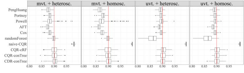
Figure 1: Empirical $90\%$ coverage of the uncensored survival time $T$. “CQR-cRF” is short for the CQR-LPB with censored quantile regression forest; “CQR-conTree” and “CDR-conTree” are short for the CQR- and CDR-LPB with distribution boosting. The other abbreviations are the same as in Table 1.

Next, we investigate the conditional coverage and efficiency of these methods. In Figure 2(a), we plot the empirical conditional coverage as a function of the conditional variance of $T$ on $X$. In particular, we stratify the data into $10$ groups based on equispaced percentiles of $\mathrm{Var}(T\mid X)$ and plot the average coverage within each stratum along with a $90\%$ confidence band obtained via repeated sampling. Note that in either the homoscedastic or the heteroscedastic case, $\mathrm{Var}(T\mid X)$ is varying with $X$. Not surprisingly, the naive CQR is conditionally conservative. In the univariate case, both the CQR- and CDR-LPB approximately achieve desired conditional coverage; in the multivariate case, the conditional coverage is slightly uneven, though still concentrating around the target line. Figure 2(b) presents the ratio between the LPBs and the true $\alpha$-th conditional quantile as a function of $\text{Var}(T\mid X)$. This is a measure of efficiency since the true conditional quantile is the oracle LPB. Here, we observe that naive CQR-LPBs are close to zero, confirming that they are overly conservative, while the CQR- and CDR-LPBs are fairly close to the oracle LPB, implying that both methods are relatively efficient.

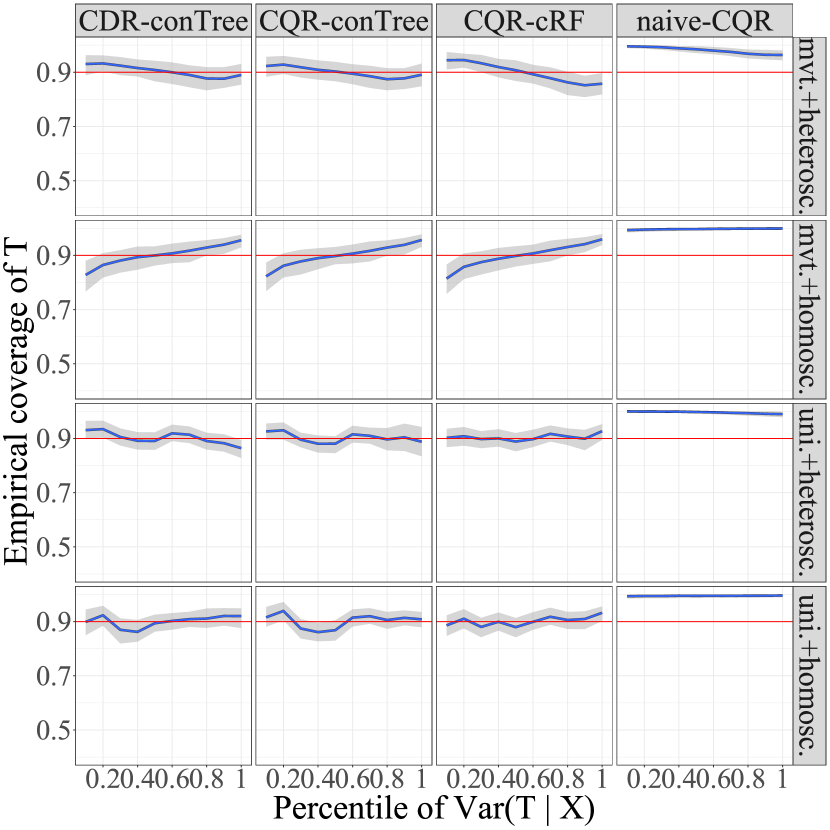
(a)

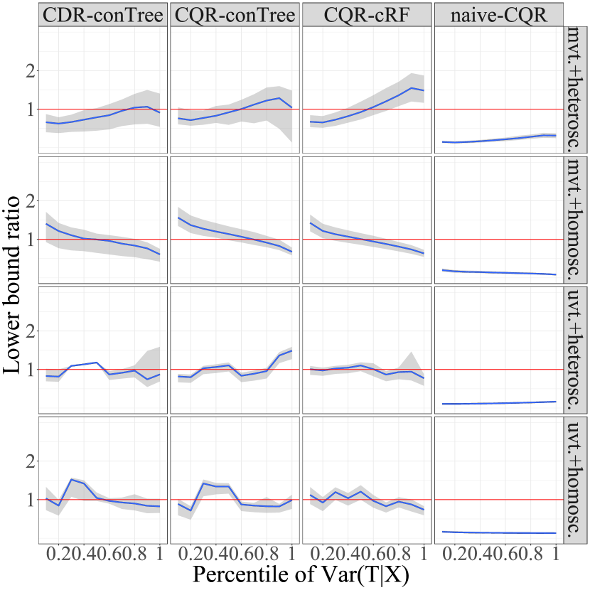
(b)

Figure 2: Results from the experiments detailed in Table 1: (a) empirical $90\%$ conditional coverage and (b) ratio between the LPB and the theoretical quantile as a function of $\text{Var}(T\mid X)$. The blue curves correspond to the mean coverage in (a) and the median ratio in (b). The gray confidence bands correspond to the $95\%$ and $5\%$ quantiles of the estimates over repeated sampling. The abbreviations are the same as in Figure 1.

5 Application to UK Biobank COVID-19 data

We apply our method to the UK Biobank COVID-19 dataset to demonstrate robustness and practicability. UK Biobank (Bycroft et al., 2018) is a large-scale biomedical database and research resource, containing in-depth genetic and health information from half a million UK participants. In April 2020, UK Biobank started to release COVID-19 testing data, and has since continued to regularly provide updates. This gives researchers access to a cohort of COVID-19 patients, along with their date of confirmation, survival status, pre-existing conditions, and other demographic covariates.

We include in our analysis all individuals in UK Biobank who received a positive COVID-19 test result before January 21st, 2021. This results in a dataset of size $n=14,\!861$ with $484$ events, defined as a COVID-related death. We extract eight covariate features, namely, age, gender, body mass index (BMI), waist size, cardiovascular disease status, diabetes status, hypothyroidism status, and respiratory disease status. As in Section 2, the censoring time is the time lapse between the date of a positive test and January 21st, 2021. The survival time is the time lapse between the date of a positive test and the event (which may have yet to occur).

We wish to harness this data to produce an LPB on the survival time of each COVID-19 patient. To apply the CQR- or CDR-LPB, we set the threshold $c_{0}$ to be $14$ days. Since survival time assessment likely informs high-stakes decision-making, we set the target level to $99\%$ for reliability.

5.1 Semi-synthetic examples

To demonstrate robustness, we start our analysis with two semi-synthetic examples so that the ground truth is known and calibration can be assessed (results on real outcomes are presented next). We keep the covariate matrix $X$ from the UK Biobank COVID-19 data. In the first simulation study, we substitute the censoring time with a synthetic $C$. In the second, each survival time, observed or not, is substituted with a synthetic version. Details follow:

• Synthetic $C$: we take the censored survival time ${\widetilde{T}}$ as the uncensored survival time and generate the censoring time $C_{\text{syn}}$ as

  $$C_{\text{syn}}\sim{\mathcal{E}}(0.001\cdot\text{age}+0.01\cdot\text{gender}).$$

  In this setting, the observables are $(X,C_{\text{syn}},{\widetilde{T}}\wedge C_{\text{syn}})$, and we wish to construct LPBs on ${\widetilde{T}}$.

• Synthetic $T$: we keep the real censoring time $C$, and generate a survival time $T_{\text{syn}}$ as:

  $$\log{T_{\text{syn}}}\mid X\sim{\mathcal{N}}(2+0.05\cdot\text{age}+0.1\cdot\text{gender},1).$$

  In this setting, the observables are $(X,C,T_{\text{syn}}\wedge C)$, and we wish to construct LPBs on $T_{\text{syn}}$.

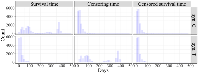
Figure 3: Histograms of the survival time, censoring time, and censored survival time defined as the minimum between the two, in each simulation setting.

Figure 3 shows the histograms of the survival time, censoring time, and censored survival time from the two simulated datasets. We apply the CDR-LPB (with $c_{0}=14$) to both. For comparison, we also apply the AFT and naive CQR. To evaluate the LPBs, we randomly split the data into a training set with $75\%$ of the data and a holdout set with the remaining $25\%$. Each method is applied to the training set, and the resulting LPBs are evaluated on the holdout set. We repeat the above procedure $100$ times to create 100 pairs of training and test data sets.

To visualize conditional calibration, we fit a Cox model on the data to generate a predicted risk score for each unit and stratify all units into $10$ subgroups defined by deciles of the predicted risk. The results for synthetic $C$ and $T$ are plotted in Figures 4 and 5, respectively. As in the simulation studies from Section 4, we see that the naive CQR is overly conservative. Notably, although the AFT-LPB is well calibrated in the synthetic-$C$ setting, this method is overly conservative in the synthetic-$T$ setting, even though the model is correctly specified. In contrast, the CDR-LPB is calibrated in both examples. From the middle panels of Figures 4 and 5, we also observe that the CDR-LPB is approximately conditionally calibrated. Finally, the right panels show that CDR-LPB nearly preserves the rank of the predicted risk given by the Cox model. The flat portion of the LPB towards the left end corresponds to the threshold, implying that at least $99\%$ of people with predicted risk scores lower than $0.5$ can survive beyond $14$ days.

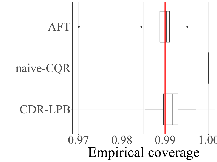
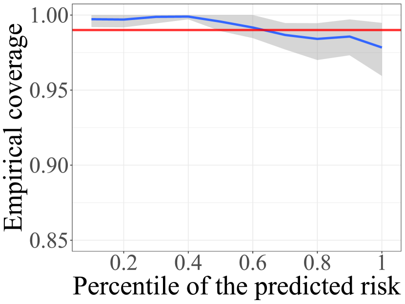
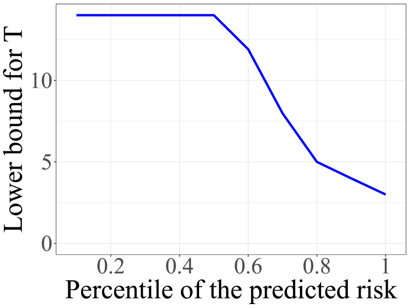
Figure 4: Results for synthetic censoring times across 100 replications: empirical coverage (left), empirical conditional coverage of the CDR-LPB (middle), and CDR-LPB as a function of the percentile of the predicted risk (right). The target coverage level is $99\%$. The blue curves correspond to the mean coverage in the middle panel and the median LPB in the right panel; the gray confidence bands correspond to the $5\%$ and $95\%$ quantiles of the estimates across $100$ independent replications.

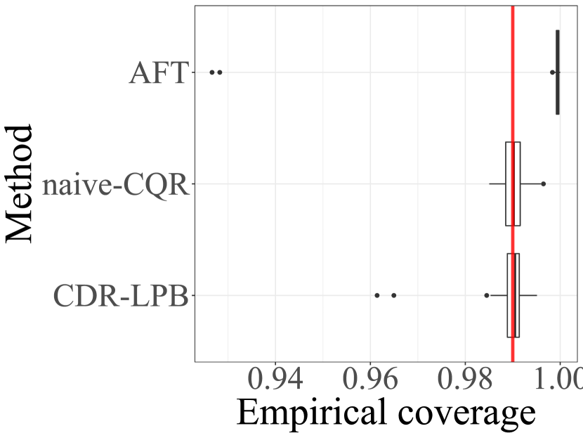
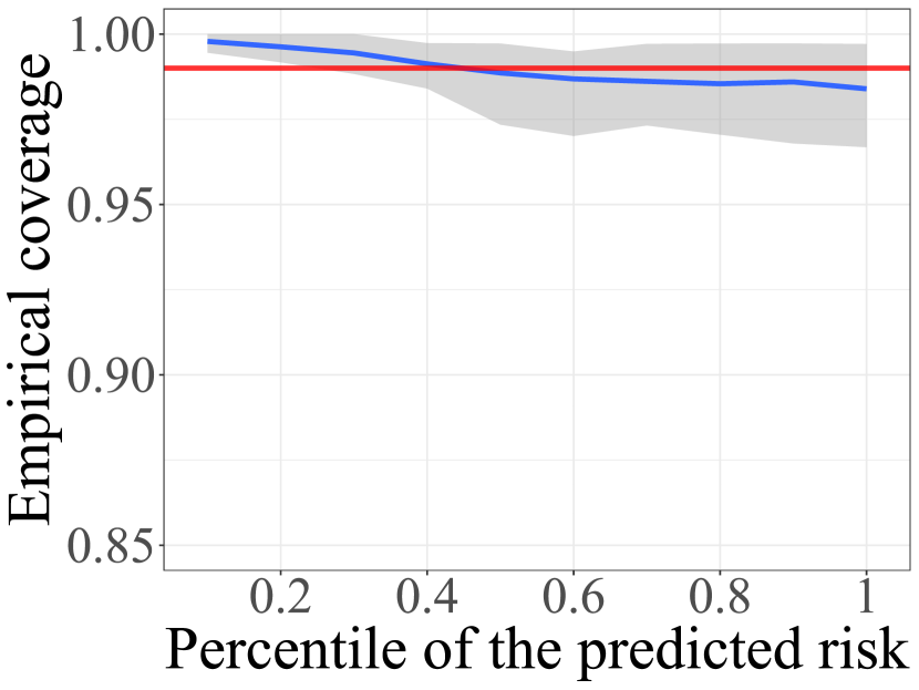
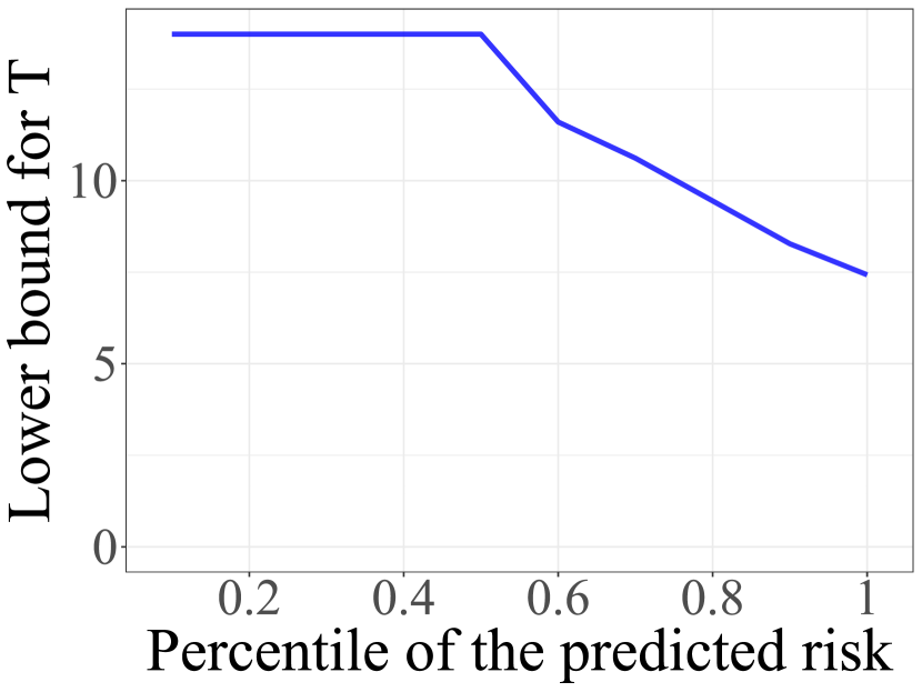
Figure 5: Results for synthetic survival times: everything else is as in Figure 4.

5.2 Real data analysis

We now turn attention to actual COVID-19 responses. Again, we randomly split the data into a training set including $75\%$ of data and a holdout set including the remaining $25\%$. Then we run the CDR on the training set and validate the LPBs on the holdout set. The issue is that the actual survival time is only partially observed, and thus, the coverage of a given LPB cannot be assessed accurately (this is precisely why we generated semi-synthetic responses in the previous section.) Nevertheless, we note that

$$\beta_{\text{lo}}:=\mathbb{P}\big{(}{\widetilde{T}}\geq\hat{L}(X)\big{)}\leq\mathbb{P}\big{(}T\geq\hat{L}(X)\big{)}\leq 1-\mathbb{P}\big{(}{\widetilde{T}}<\hat{L}(X),T\leq C\big{)}=:\beta_{\text{hi}},$$

where both $\beta_{\text{lo}}$ and $\beta_{\text{hi}}$ are estimable from the data. This says that we can assess the marginal coverage of the LPBs by evaluating a lower and upper bound on the coverage. Of course, this extends to conditional coverage.

To assess the stability, we evaluate our method on $100$ independent sample splits. Figure 6 presents the empirical lower and upper bound of the marginal coverage and those of the conditional coverage as functions of the predicted risk (as in the semi-synthetic examples), together with their variability across $100$ sample splits. The left panel shows that the upper bound is very close to the lower bound, and both concentrate around the target level. Thus we can be assured that the CDR-LPB is well calibrated. Similarly, the other panels show that the CDR-LPB is approximately conditionally calibrated. We conclude this section by showing in Figure 7 the LPBs as functions of the percentiles of the predicted risk, age, and BMI, respectively.

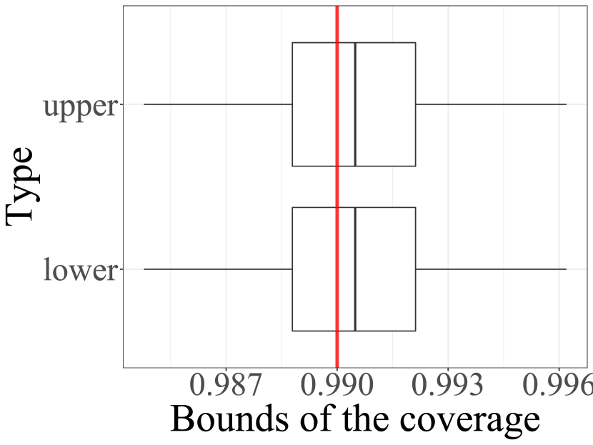
(a)

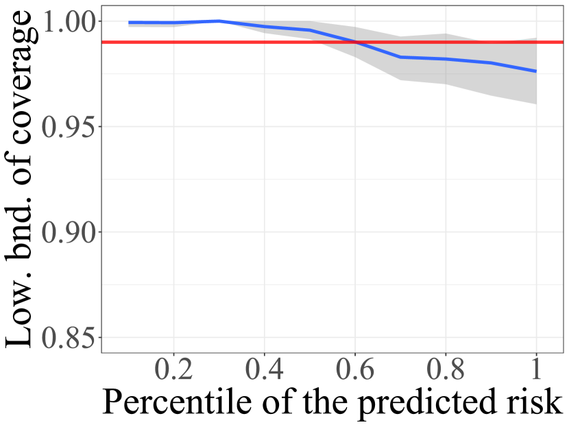
(b)

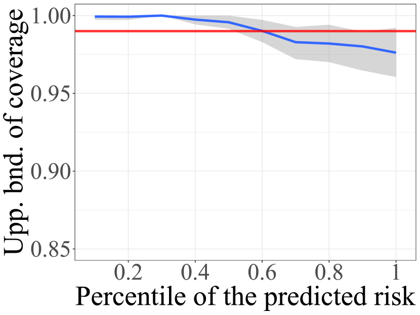
(c)

Figure 6: Analysis of the UK Biobank COVID-19 data: (a) lower and upper bounds of the empirical coverage; (b) lower and (c) upper bounds of empirical coverage as a function of the predicted risk. The target coverage level is $99\%$. The blue curves correspond to the mean coverage, and the gray confidence bands correspond to the $5\%$ and $95\%$ quantiles of the estimates across $100$ sample splits.

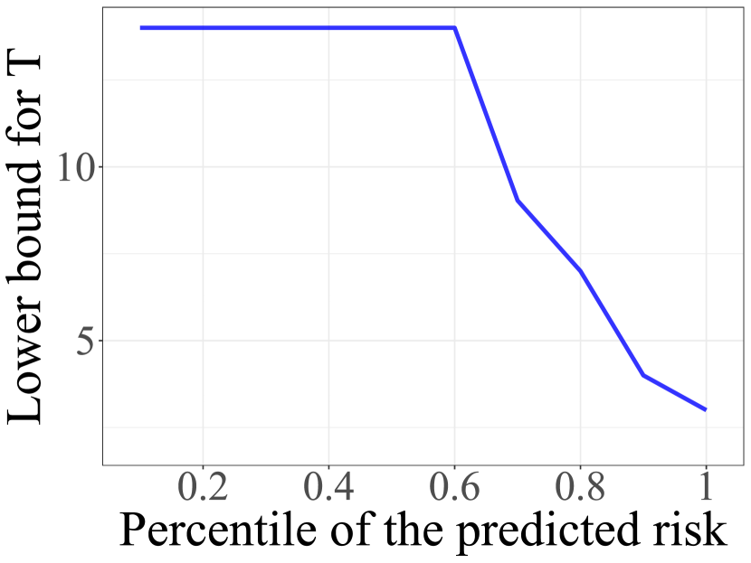
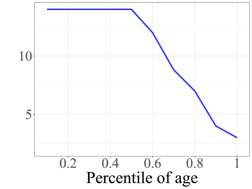
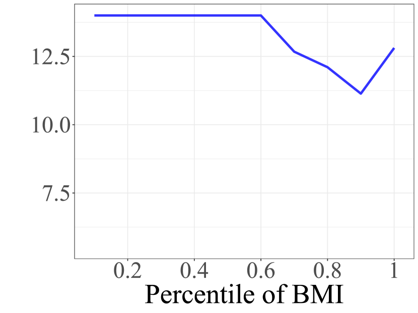
Figure 7: Analysis of the UK Biobank COVID-19 data: LPBs on the survival time of COVID-19 patients as a function of the percentiles of predicted risk (left), age (middle) and BMI (right). The target coverage level is $99\%$. The blue curves correspond to the median LPB across $100$ sample splits.

6 Discussion and extensions

6.1 Beyond Type-I censoring

In practice, censoring can be driven by multiple factors. As discussed in Leung et al. (1997), the two most common types of right censoring in a clinical study are the end-of-study censoring caused by the trial termination and the loss-to-follow-up censoring caused by unexpected attrition; see also Korn (1986) and Schemper and Smith (1996) for an account of the two types of censoring. Let $C_{\mathrm{end}}$ denote the former and $C_{\mathrm{loss}}$ the latter. By definition, $C_{\mathrm{end}}$ is observable for every patient, as long as the entry times are accurately recorded. When the event is not death (e.g., the patient’s returning visit), $C_{\mathrm{loss}}$ is observable if all patients are tracked until the end of the study. However, when the event is death, $C_{\mathrm{loss}}$ can only be observed for surviving patients. This is because for dead patients, it is impossible to know when they would have been lost to follow-up, had they survived.

In survival analysis without loss-to-follow-up censoring, or time-to-event analysis with non-death events, the setting of Type I censoring considered in this paper is plausible. However, it is found that both the end-of-study and loss-to-follow-up censoring are involved in many applications (Leung et al., 1997). In these cases, the effective censoring time $C$ is the minimum of $C_{\mathrm{end}}$ and $C_{\mathrm{loss}}$, and is only observable for surviving patients, namely the patients with $T>C$. This situation prevents us from applying Algorithm 1 below because the subpopulation with $C\geq c_{0}$ is not fully observed. If we use the subpopulation whose $C$ is 1) observed and 2) larger than or equal to a threshold $c_{0}$ instead, then the joint distribution of $(X,T)$ becomes $P_{X\mid C\geq c_{0},T>C}\times P_{T\mid X,C\geq c_{0},T>C}$. The extra conditioning event $T>C$ induces a shift of the conditional distribution, since $P_{T\mid X,C\geq c_{0},T>C}\neq P_{T\mid X,C\geq c_{0}}$ in general, rendering the weighted split conformal inference invalid.

Our method can nevertheless be adapted to yield meaningful inference under an additional assumption:

$$(T,C_{\mathrm{loss}})~{}\rotatebox[origin={c}]{90.0}{$\models$}~{}C_{\mathrm{end}}\mid X.$$ (12)

Unlike Korn (1986) and Schemper and Smith (1996), (12) does not impose any restrictions on the dependence between $T$ and $C_{\mathrm{loss}}$, which is harder to conceptualize. The assumption (12) tends to be plausible, especially when the total length of follow-up is short, since the randomness of the end-of-study censoring time often comes from the entry time of a patient, which is arguably exogenous to the survival time and attrition, at least when conditioning on a few demographic variables. There are certain cases where (12) could be violated. For example, if new treatments become available during the course of a study, subjects who enter later are different from those who enter earlier as they could have been given the alternative treatments, but were not.

Let $T^{\prime}=T\wedge C_{\mathrm{loss}}$, the survival time censored merely by the loss to follow-up. Then the censored survival time $\tilde{T}=T\wedge C=T^{\prime}\wedge C_{\mathrm{end}}$, and (12) implies that $T^{\prime}\rotatebox[origin={c}]{90.0}{$\models$}C_{\mathrm{end}}\mid X$, an analog of the conditionally independent censoring assumption (1). Since $C_{\mathrm{end}}$ is observed for every patient, Algorithm 1 can be applied to produce an LPB $\hat{L}(\cdot)$ such that

$$\mathbb{P}(T^{\prime}\geq\hat{L}(X))\geq 1-\alpha\Longrightarrow\mathbb{P}(T\geq\hat{L}(X))\geq 1-\alpha.$$

In Section D.5 of the Appendix, we provide an additional simulation illustrating the result of our method in this setting. An observation in conjunction with this line of reasoning is that, unlike most survival analysis techniques, our method distinguishes two sources of censoring and takes advantage of the censoring mechanism itself. It can be regarded as a building block to remove the adverse effect of $C_{\mathrm{end}}$. It remains an interesting question whether the censoring issue induced by $C_{\mathrm{loss}}$ can be resolved or alleviated in this context.

6.2 Sharper coverage criteria

It is more desirable to achieve a stronger conditional coverage criterion:

$$\mathbb{P}\left(T\geq\hat{L}(X)\mid X=x\right)\geq 1-\alpha,$$ (13)

which states that $\hat{L}(X)$ is a conditionally calibrated LPB. Clearly, (13) implies valid marginal coverage. Theorem 2 and 3 show that the CQR- and CDR-LPB are approximately conditionally calibrated if the conditional quantiles are estimated well. However, without distributional assumptions, we can show that (13) can only be achieved by trivial LPBs.

Theorem 5

Assume that $X\in\mathbb{R}^{p}$ and $C\geq 0,T\geq 0$. Let $P_{(X,C)}$ be any given distribution of $(X,C)$. If $\hat{L}(\cdot)$ satisfies (13) uniformly for all joint distributions of $(X,C,T)$ with $(X,C)\sim P_{(X,C)}$, then for all such distributions,

$$\mathbb{P}(\hat{L}(x)=0)\geq 1-\alpha,$$

at almost surely all points $x$ aside from the atoms of $P_{X}$.

Theorem 5 implies that no nontrivial LPB exists even if the distribution of $(X,C)$ is known. Put another way, it is impossible to achieve desired conditional coverage while being agnostic to the conditional survival function. This impossibility result is inspired by previous works on uncensored outcomes and two-sided intervals (Vovk, 2012; Barber et al., 2019a).

It is valuable to find other achievable coverage criteria which are sharper than the marginal coverage criterion (3). Without censoring and covariate shift, Vovk et al. (2003) introduced Mondrian conformal inference to achieve desired marginal coverage over multiple subpopulations. The idea is further developed from different perspectives (Vovk, 2012; Lei et al., 2013; Guan, 2019; Barber et al., 2019a; Romano et al., 2019a). Given a partition of the covariate space $\{{\mathcal{X}}_{1},\ldots,{\mathcal{X}}_{K}\}$, Mondrian conformal inference guarantees that

$$\mathbb{P}(Y\in\hat{C}(X)\mid X\in{\mathcal{X}}_{k})\geq 1-\alpha,\quad k=1,\ldots,K.$$

Mondrian conformal inference allows the subgroups to also depend on the outcome; see Vovk et al. (2005), which refers to the rule of forming subgroups as a “taxonomy.” Besides, the subgroups can also be overlapping; see Barber et al. (2019a). Following their techniques, we can extend Mondrian conformal inference to our case by modifying the calibration term $\eta(x)$ (in Algorithm 1):

$$\eta(x)=\mathrm{Quantile}\left(1-\alpha;\frac{\sum_{i\in{\mathcal{I}}_{\text{ca}},X_{i}\in{\mathcal{X}}_{k}}\hat{p}_{i}(x)\delta_{V_{i}}+\hat{p}_{\infty}(x)\delta_{\infty}}{\sum_{i\in{\mathcal{I}}_{\text{ca},X_{i}\in{\mathcal{X}}_{k}}}\hat{p}_{i}(x)+\hat{p}_{\infty}(x)}\right),\quad\forall x\in{\mathcal{X}}_{k}.$$ (14)

Suppose ${\mathcal{X}}_{1}$ and ${\mathcal{X}}_{2}$ correspond to male and female subpopulations. Then $\eta(x)$ is a function of both the testing point $x$ and the gender. That said, estimation of censoring mechanisms and conditional survival functions can still depend on the whole training fold ${\mathcal{Z}}_{\mathrm{tr}}$ as joint training may be more powerful than separate training on each subpopulation (Romano et al., 2019a).

When the censoring mechanism is known, we can prove that

$$\mathbb{P}(T\wedge c_{0}\geq\hat{L}(X)\mid X\in{\mathcal{X}}_{k})\geq 1-\alpha,\quad k=1,\ldots,K.$$ (15)

By the conditionally independent censoring assumption, the target distribution in the localized criterion (15) for a given $k$ can be rewritten as

$$(X,T\wedge c_{0})\mid C\geq c_{0},X\in{\mathcal{X}}_{k}~{}\sim~{}P_{X\mid C\geq c_{0},X\in{\mathcal{X}}_{k}}\times P_{T\wedge c_{0}\mid X}.$$ (16)

The covariate shift between the observed and target distributions is

$$w_{k}(x)=\frac{dP_{X\mid C\geq c_{0},X\in{\mathcal{X}}_{k}}}{dP_{X}}(x)\propto\frac{I(x\in{\mathcal{X}}_{k})}{\mathbb{P}(C\geq c_{0}\mid X=x)}.$$

This justifies the calibration term (14) in the weighted Mondrian conformal inference. Since the weighted Mondrian conformal inference is a special case of Algorithm 1, it also enjoys the double robustness property, implied by Theorem B.4 in Section B in the Appendix.

6.3 Survival counterfactual prediction

The proposed method in this paper is designed for a single cohort. In practice, patients are often exposed to multiple conditions, and the goal is to predict the counterfactual survival times had the cohort been exposed to a different condition. For example, a clinical study typically involves a treatment group and a control group. For a new patient, it is of interest to predict her survival time had she been assigned the treatment. For uncensored outcomes, Lei and Candès (2021) proposed a method based on weighted conformal inference for counterfactual prediction under the potential outcome framework (Neyman, 1923/1990; Rubin, 1974). We can extend their strategy to handle censored outcomes and apply it to the survival counterfactual prediction.

Suppose each patient has a pair of potential survival times $(T(1),T(0))$, where $T(1)$ (resp. $T(0)$) denotes the survival time had the patient been assigned into the treatment (resp. control) group. Our goal is to construct a calibrated LPB on $T(1)$, given i.i.d. observations $(X_{i},W_{i},C_{i},T_{i})_{i=1}^{n}$ with $W_{i}$ denoting the treatment assignment and

$$T_{i}=\left\{\begin{array}[]{ll}T_{i}(1),&W_{i}=1,\\ T_{i}(0),&W_{i}=0.\end{array}\right.$$

Without further assumptions on the correlation structures between $T(1)$ and $T(0)$, it is natural to conduct inference based on the observed treated group since the control group contains no information about $T(1)$. The joint distribution of $(X,T(1)\wedge c_{0})$ on this group becomes

$$(X,T(1)\wedge c_{0})\mid C\geq c_{0},W=1~{}\sim~{}P_{X\mid C\geq c_{0},W=1}\times P_{T(1)\wedge c_{0}\mid X,C\geq c_{0},W=1}.$$

Under the assumption that $(T(1),T(0))\rotatebox[origin={c}]{90.0}{$\models$}(W,C)\mid X$, the conditional distribution of $T(1)\wedge c_{0}$ matches the target:

$$P_{T(1)\wedge c_{0}\mid X,C\geq c_{0},W=1}=P_{T(1)\wedge c_{0}\mid X}.$$

The assumption is a combination of the strong ignorability assumption (Rubin, 1978), a widely accepted starting point in causal inference, and the conditionally independent censoring assumption. The density ratio of the two covariate distributions can be characterized by

$$w(x)=\frac{dP_{X\mid C\geq c_{0},W=1}}{dP_{X}}(x)\propto\frac{1}{\mathbb{P}(C\geq c_{0},W=1\mid X=x)}.$$

In many applications, it is plausible to further assume that $C\rotatebox[origin={c}]{90.0}{$\models$}W\mid X$. In this case,

$$\mathbb{P}(C\geq c_{0},W=1\mid X=x)=\mathbb{P}(C\geq c_{0}\mid X=x)\mathbb{P}(W=1\mid X=x),$$

where the first term is the censoring mechanism and the second term is the propensity score (Rosenbaum and Rubin, 1983). Therefore, we can obtain calibrated LPBs on counterfactual survival times if both the censoring mechanism and the propensity score are known. This assumption is often plausible for randomized clinical trials. Furthermore, it has a doubly robust guarantee of coverage that is similar to Theorems 2 and 3.

Acknowledgment

E. C. was supported by Office of Naval Research grant N00014-20-12157, by the National Science Foundation grants OAC 1934578 and DMS 2032014, by the Army Research Office (ARO) under grant W911NF-17-1-0304, and by the Simons Foundation under award 814641. L. L. and Z. R. were supported by the same NSF OAC grant and by the Discovery Innovation Fund for Biomedical Data Sciences. L.L. was also supported by NIH grant R01MH113078. The authors are grateful to Steven Goodman, Lucas Janson, Ying Jin, Yan Min, Chiara Sabatti, Matteo Sesia, Lu Tian and Steve Yadlowsky for their constructive feedback. This research has been conducted using the UK Biobank Resource under Application Number 27837.

Appendix A Proofs of impossibility results

A.1 Proof of Theorem 1

Let $(X_{i},C_{i},T_{i})_{i=1}^{n+1}\stackrel{{\scriptstyle i.i.d.}}{{\sim}}(X,C,T)$. For notational convenience, we put $Z_{i}=(X_{i},C_{i},T_{i})$. To avoid confusion, we expand $\hat{L}(x)$ into $\hat{L}(Z_{1},\ldots,Z_{n};x)$. Note that $\hat{L}$ depends on $(Z_{1},\ldots,Z_{n})$ through $(X_{i},C_{i},{\widetilde{T}}_{i})_{i=1}^{n}$. Let

$$\phi(Z_{1},\ldots,Z_{n+1})=I(T_{n+1}<\hat{L}_{n}(Z_{1},\ldots,Z_{n};X_{n+1})).$$

Since $\hat{L}_{n}$ satisfies (3) under the conditionally independent censoring assumption (1), we have that

$$\mathbb{P}\left(\phi(Z_{1},\ldots,Z_{n+1})=1\right)\leq\alpha.$$

As a result, if we treat $T\rotatebox[origin={c}]{90.0}{$\models$}C\mid X$ as a null hypothesis, $\phi(Z_{1},\ldots,Z_{n+1})$ is an $\alpha$-level test. Note that $X$ is continuous, and $(T,C)$ are continuous or discrete. By Theorem 2 and Remark 4 of Shah et al. (2020), for any joint distribution $Q$ of $Z$ with the same continuity conditions on $(X,C,T)$,

$$\mathbb{P}_{Z_{i}\stackrel{{\scriptstyle i.i.d.}}{{\sim}}Q}\left(\phi(Z_{1},\ldots,Z_{n+1})=1\right)\leq\alpha.$$ (A.1)

Let $\tilde{Z}_{i}=(X_{i},C_{i},{\widetilde{T}}_{i})$ and $Q$ denote its distribution. Then ${\widetilde{T}}_{i}\wedge C_{i}=T_{i}\wedge C_{i}$ and thus

$$\hat{L}_{n}(\tilde{Z}_{1},\ldots,\tilde{Z}_{n};x)=\hat{L}_{n}(Z_{1},\ldots,Z_{n};x).$$

Clearly, $X$ is absolutely continuous with respect to the Lebesgue measure and ${\widetilde{T}},C$ are absolutely continuous with respect to the Lebesgue measure or the counting measure. By (A.1) and the definition of $\phi$, we have

$$\mathbb{P}\left(\tilde{T}_{n+1}\geq\hat{L}_{n}(Z_{1},\ldots,Z_{n};X_{n+1})\right)\geq 1-\alpha.$$

The proof is then completed by replacing $(T_{n+1},X_{n+1})$ with $(T,X)$.

A.2 Proof of Theorem 5

We prove the theorem by modifying the proof of Proposition 4 from Vovk (2012). To avoid confusion, we expand $\hat{L}(x)$ into $\hat{L}(Z_{1},\ldots,Z_{n};x)$ where $Z_{i}=(X_{i},C_{i},{\widetilde{T}}_{i})$. Fix any distribution $P$ with $(X,C)\sim P_{(X,C)}$ and $C\geq 0,T\geq 0$ almost surely. Suppose there exists a set $\mathcal{V}$ of $P_{X}$-non-atom $x$ such that $P_{X}(\mathcal{V})>0$, and for any $x\in\mathcal{V}$,

$$\mathbb{P}_{Z_{i}\stackrel{{\scriptstyle i.i.d.}}{{\sim}}P}(\hat{L}(Z_{1},\ldots,Z_{n},x)>0)>\alpha.$$

Since $\mathcal{V}$ only includes non-atom $x$’s, there exists $t_{0}>0$ and $\delta>0$ such that

$$\mathbb{P}_{Z_{i}\stackrel{{\scriptstyle i.i.d.}}{{\sim}}P}(\hat{L}(x)>t_{0})>\alpha+\delta,\quad\forall x\in\mathcal{V}.$$ (A.2)

We can further shrink $\mathcal{V}$ so that

$$\sqrt{2-2(1-P_{X}(\mathcal{V}))^{n}}\leq\delta/2.$$ (A.3)

Fix any $t_{1}\in(0,t_{0})$. Define a new probability distribution $Q$ on $(X,C,T)$ with $(X,C)\sim P_{(X,C)}$ and the regular conditional probability

$$Q(T\in A\mid X=x,C=c)=\left\{\begin{array}[]{ll}P(T\in A\mid X=x,C=c),&x\not\in\mathcal{V},\\ \delta_{t_{1}}(A),&x\in\mathcal{V},\end{array}\right.$$

where $\delta_{t_{1}}$ defines the point mass on $t_{1}$. Let $d_{\mathrm{TV}}$ denote the total-variation distance. Then,

$$d_{\mathrm{TV}}(P,Q) =\sup_{{\mathcal{A}}_{X},{\mathcal{A}}_{C},{\mathcal{A}}_{T}}|P(X\in{\mathcal{A}}_{X},C\in{\mathcal{A}}_{C},T\in{\mathcal{A}}_{T})-Q(X\in{\mathcal{A}}_{X},C\in{\mathcal{A}}_{C},T\in{\mathcal{A}}_{T})|$$ (A.4)

$$=\sup_{{\mathcal{A}}_{X},{\mathcal{A}}_{C},{\mathcal{A}}_{T}}|P(X\in{\mathcal{A}}_{X}\cap\mathcal{V},C\in{\mathcal{A}}_{C},T\in{\mathcal{A}}_{T})-Q(X\in{\mathcal{A}}_{X}\cap\mathcal{V},C\in{\mathcal{A}}_{C},T\in{\mathcal{A}}_{T})|$$ (A.5)

$$\leq\sup_{{\mathcal{A}}_{X},{\mathcal{A}}_{C},{\mathcal{A}}_{T}}\max\{P(X\in{\mathcal{A}}_{X}\cap\mathcal{V},C\in{\mathcal{A}}_{C},T\in{\mathcal{A}}_{T}),Q(X\in{\mathcal{A}}_{X}\cap\mathcal{V},C\in{\mathcal{A}}_{C},T\in{\mathcal{A}}_{T})\}$$ (A.6)

$$\leq\sup_{{\mathcal{A}}_{X}}\max\{P(X\in{\mathcal{A}}_{X}\cap\mathcal{V}),Q(X\in{\mathcal{A}}_{X}\cap\mathcal{V})\}$$ (A.7)

$$=\sup_{{\mathcal{A}}_{X}}P_{X}({\mathcal{A}}_{X}\cap\mathcal{V})\leq P_{X}(\mathcal{V}).$$ (A.8)

Using the tensorization inequality for the total-variation distance (see e.g., Tsybakov (2008), Section 2.4) and (A.3), we obtain that

$$d_{\mathrm{TV}}(P^{n},Q^{n})\leq\sqrt{2-2(1-d_{\mathrm{TV}}(P,Q))^{n}}\leq\delta/2.$$

Together with (A.2), this implies that

$$\mathbb{P}_{Z_{i}\stackrel{{\scriptstyle i.i.d.}}{{\sim}}Q}(\hat{L}(x)>t_{0})>\alpha+\delta/2,\quad\forall x\in\mathcal{V}.$$

Let $Z=(X,C,T)$ be an independent draw from $Q$. The above inequality can be reformulated as

$$\mathbb{P}_{Z_{i},Z\stackrel{{\scriptstyle i.i.d.}}{{\sim}}Q}(\hat{L}(X)>t_{0}\mid X=x)>\alpha+\delta/2,\quad\forall x\in\mathcal{V}.$$

Marginalizing over $x\in\mathcal{V}$, it implies that

$$\mathbb{P}_{Z_{i},Z\stackrel{{\scriptstyle i.i.d.}}{{\sim}}Q}(\hat{L}(X)>t_{0},X\in\mathcal{V})>(\alpha+\delta/2)Q_{X}(\mathcal{V}).$$ (A.9)

By definition of $Q$, $T=t_{1}<t_{0}$ almost surely conditional on $X\in\mathcal{V}$. Thus,

$$\mathbb{P}_{Z_{i},Z\stackrel{{\scriptstyle i.i.d.}}{{\sim}}Q}(T<\hat{L}(X),X\in\mathcal{V})>(\alpha+\delta/2)Q_{X}(\mathcal{V}).$$

On the other hand, since $Q$ is a distribution with the same marginal distribution of $(X,C)$ and $T\geq 0$ almost surely, for any $x$,

$$\mathbb{P}_{Z_{i},Z\stackrel{{\scriptstyle i.i.d.}}{{\sim}}Q}(T<\hat{L}(X)\mid X=x)\leq\alpha.$$

Marginalizing over $x\in\mathcal{V}$, it implies that

$$\mathbb{P}_{Z_{i},Z\stackrel{{\scriptstyle i.i.d.}}{{\sim}}Q}(T<\hat{L}(X),X\in\mathcal{V})\leq\alpha Q_{X}(\mathcal{V}).$$

This contradicts (A.9) since $Q_{X}(\mathcal{V})=P_{X}(\mathcal{V})>0$. The theorem is proved by contradiction.

Appendix B Double robustness of weighted conformal inference

Throughout this section, we will focus on the generic weighted conformal inference sketched in Algorithm 2 below.

Input: level $\alpha$; data ${\mathcal{Z}}=(X_{i},Y_{i})_{i\in{\mathcal{I}}}$; testing point $x$;

           function $V(x,y;{\mathcal{D}})$ to compute the conformity score between $(x,y)$ and data ${\mathcal{D}}$;

           function $\hat{w}(x;{\mathcal{D}})$ to fit the weight function at $x$ using ${\mathcal{D}}$ as data.

Procedure:

   1. Split ${\mathcal{Z}}$ into a training fold ${\mathcal{Z}}_{\text{tr}}\triangleq(X_{i},Y_{i})_{i\in{\mathcal{I}}_{\text{tr}}}$ and a calibration fold ${\mathcal{Z}}_{\text{ca}}\triangleq(X_{i},Y_{i})_{i\in{\mathcal{I}}_{\text{ca}}}$.

   2. For each $i\in{\mathcal{I}}_{\text{ca}}$, compute the conformity score $V_{i}=V(X_{i},Y_{i};{\mathcal{Z}}_{\text{tr}})$.

   3. For each $i\in{\mathcal{I}}_{\text{ca}}$, compute the weight $W_{i}=\hat{w}(X_{i};{\mathcal{Z}}_{\text{tr}})\in[0,\infty)$.

   4. Compute the weights $\hat{p}_{i}(x)=\frac{W_{i}}{\sum_{i\in{\mathcal{I}}_{\text{ca}}}W_{i}+\hat{w}(x;{\mathcal{Z}}_{\text{tr}})}$ and $\hat{p}_{\infty}(x)=\frac{\hat{w}(x;{\mathcal{Z}}_{\text{tr}})}{\sum_{i\in{\mathcal{I}}_{\text{ca}}}W_{i}+\hat{w}(x;{\mathcal{Z}}_{\text{tr}})}$.

   5. Compute $\eta(x)=\mathrm{Quantile}\left(1-\alpha;\sum_{i\in{\mathcal{I}}_{\text{ca}}}\hat{p}_{i}(x)\delta_{V_{i}}+\hat{p}_{\infty}(x)\delta_{\infty}\right)$.

Output: $\hat{L}(x)=\inf\{y:V(x,y;{\mathcal{Z}}_{\text{tr}})\leq\eta(x)\}$

Algorithm 2 generic weighted split conformal inference

B.1 Conformity score via nested sets

Gupta et al. (2019) introduced a broad class of conformity scores characterized by nested sets. Suppose we have a totally ordered index set ${\mathcal{S}}$ (e.g., $\mathbb{R}$) and a sequence of nested sets $\{{\mathcal{F}}_{s}(x;{\mathcal{D}}):s\in{\mathcal{S}}\}$ in the sense that ${\mathcal{F}}_{s_{1}}(x;{\mathcal{D}})\subset{\mathcal{F}}_{s_{2}}(x;{\mathcal{D}})$ for any $s_{1}\leq s_{2}\in{\mathcal{S}}$. Define a score as the index of the minimal set that includes $y$, i.e.

$$V(x,y;{\mathcal{D}})=\inf\{s\in{\mathcal{S}}:y\in{\mathcal{F}}_{s}(x;{\mathcal{D}})\}.$$ (B.1)

Without loss of generality, we assume throughout that ${\mathcal{F}}_{\inf{\mathcal{S}}}(x)$ is the empty set and ${\mathcal{F}}_{\sup{\mathcal{S}}}(x)$ is the full domain of $Y$. The CMR-, CQR-, and CDR-based scores are instances of this:

• CMR score: ${\mathcal{F}}_{s}(x;{\mathcal{D}})=[\hat{m}(x)-s,\infty)$.

• CQR score: ${\mathcal{F}}_{s}(x;{\mathcal{D}})=[\hat{q}_{\alpha}(x)-s,\infty)$.

• CDR score: ${\mathcal{F}}_{s}(x;{\mathcal{D}})=[\hat{q}_{\alpha-s}(x),\infty)$.

We refer the readers to Table 1 of Gupta et al. (2019) for a list of other conformity scores.

B.2 Nonasymptotic theory for weighted conformal inference

In this section, we establish nonasymptotic bounds for the coverage which would imply the asymptotic results (e.g., Theorem 2 and Theorem 3), formally proved in Section C. The first result is identical to Theorem A.1 of Lei and Candès (2021).

Theorem B.1

Let $(X_{i},Y_{i})\stackrel{{\scriptstyle i.i.d.}}{{\sim}}(X,Y)\sim P_{X}\times P_{Y\mid X}$ and $Q_{X}$ be another distribution on the domain of $X$. Set $N=|\mathcal{Z}_{\mathrm{tr}}|$ and $n=|\mathcal{Z}_{\mathrm{ca}}|$. Further, let $\hat{w}(x)=\hat{w}(x;\mathcal{Z}_{\mathrm{tr}})$ be an estimate of $w(x)=(dQ_{X}/dP_{X})(x)$, and $\hat{C}(x)$ be the conformal interval resulting from Algorithm 2 with an arbitrary conformity score (not necessarily the ones defined in Section B.1). Assume that $\mathbb{E}[\hat{w}(X)\mid\mathcal{Z}_{\mathrm{tr}}]<\infty$, where $\mathbb{E}$ denotes expectation over $X\sim P_{X}$. Redefine $\hat{w}(x)$ as $\hat{w}(x)/\mathbb{E}[\hat{w}(X)\mid\mathcal{Z}_{\mathrm{tr}}]$ so that $\mathbb{E}[\hat{w}(X)\mid\mathcal{Z}_{\mathrm{tr}}]=1$. Then

$$\mathbb{P}_{(X,Y)\sim Q_{X}\times P_{Y\mid X}}\left(Y\in\hat{C}(X)\right)\geq 1-\alpha-\frac{1}{2}\mathbb{E}_{X\sim P_{X}}\big{[}|\hat{w}(X)-w(X)|\big{]}.$$ (B.2)

The second result generalizes Theorem A.2 of Lei and Candès (2021).

Theorem B.2

In the setting of Theorem B.1, assume further that

1. $\mathbb{P}_{X\sim Q_{X}}(w(X)<\infty)=1$, and there exist $\delta,M>0$ such that $\left(\mathbb{E}\left[\hat{w}(X)^{1+\delta}\right]\right)^{1/(1+\delta)}\leq M$;

2. There exists $r>0,s_{0}\in{\mathcal{S}}$, $b_{2}>b_{1}>0$, and a sequence of oracle nested sets $\{{\mathcal{O}}_{s}(x)\}_{s\in{\mathcal{S}}}$, such that

   1. for any $\varepsilon\in[0,r]$,

      $$1-\alpha-b_{2}\varepsilon\leq\mathbb{P}\left(Y\in{\mathcal{O}}_{s_{0}-\varepsilon}(X)\mid X\right)\leq 1-\alpha-b_{1}\varepsilon,\quad\text{almost surely};$$ (B.3)

   2. there exist $k,\ell>0$ such that $\displaystyle\lim_{N\rightarrow\infty}\mathbb{E}[\hat{w}(X)\Delta^{k}(X)]=\lim_{N\rightarrow\infty}\mathbb{E}[w(X)\Delta^{\ell}(X)]=0$, where $\Delta(x)=\sup_{s\in[s_{0}-r,s_{0}]}~{}\Delta_{s}(x)$, and

      $$\Delta_{s}(x)=\inf\left\{\Delta\geq 0:s-\Delta\in{\mathcal{S}},{\mathcal{F}}_{s-\Delta}(x;{\mathcal{Z}}_{\mathrm{tr}})\subset{\mathcal{O}}_{s}(x)\text{ and }{\mathcal{O}}_{s-\Delta}(x)\subset{\mathcal{F}}_{s}(x;{\mathcal{Z}}_{\mathrm{tr}})\right\}.$$ (B.4)

Then there are constants $B_{1}$ and $B_{2}$ that only depend on $r,b_{1},b_{2},\delta,M,k,\ell$ such that

$$\mathbb{P}_{(X,Y)\sim Q_{X}\times P_{Y\mid X}}(Y\in\hat{C}(X))\geq 1-\alpha\\ -B_{1}\left\{\frac{(\log n)^{(1+\delta^{\prime})/2(2+\delta^{\prime})}}{n^{\delta^{\prime}/(2+\delta^{\prime})}}+\left(\mathbb{E}[\hat{w}(X)\Delta^{k}(X)]\right)^{1/(2+k)}+\left(\mathbb{E}[w(X)\Delta^{\ell}(X)]\right)^{1/(1+\ell)}\right\},$$ (B.5)

and, with probability at least $1-\beta$,

$$\mathbb{P}_{(X,Y)\sim Q_{X}\times P_{Y\mid X}}(Y\in\hat{C}(X)\mid X)\geq 1-\alpha\\ -B_{2}\left\{\frac{(\log n)^{(1+\delta^{\prime})/2(2+\delta^{\prime})}}{n^{\delta^{\prime}/(2+\delta^{\prime})}}+\left(\mathbb{E}[\hat{w}(X)\Delta^{k}(X)]\right)^{1/(2+k)}+\left(\frac{\mathbb{E}[w(X)\Delta^{\ell}(X)]}{\beta}\right)^{1/\ell}\right\}.$$ (B.6)

where $\delta^{\prime}=\min\{\delta,1\}$. In particular, $B_{1}$ and $B_{2}$ depends on $M$ polynomially.

The next theorem shows that the conformal prediction interval is approximately the oracle interval when the outcome model is well estimated.

Theorem B.3

In the setting of Theorem B.1, assume further that

1. There exist $\delta_{0},\delta,M>0$ such that $\left(\mathbb{E}\left[w(X)^{1+\delta_{0}}\right]\right)^{1/(1+\delta_{0})}\leq M,\left(\mathbb{E}\left[\hat{w}(X)^{1+\delta}\right]\right)^{1/(1+\delta)}\leq M$;

2. There exists $r>0,s_{0}\in{\mathcal{S}}$, $b_{1}>0$, and a sequence of oracle nested sets $\{{\mathcal{O}}_{s}(x)\}_{s\in{\mathcal{S}}}$, such that

   1. for any $\varepsilon\in[0,r]$,

      $$\mathbb{P}\left(Y\in{\mathcal{O}}_{s_{0}+\varepsilon}(X)\mid X\right)\geq 1-\alpha+b_{1}\varepsilon,\quad\text{almost surely};$$ (B.7)

   2. there exist $k,\ell>0$ such that $\displaystyle\lim_{N\rightarrow\infty}\mathbb{E}[\hat{w}(X)\Delta^{{}^{\prime}k}(X)]=\lim_{N\rightarrow\infty}\mathbb{E}[w(X)\Delta^{{}^{\prime}\ell}(X)]=0$, where $\Delta^{\prime}(x)=\sup_{s\in[s_{0},s_{0}+r]}~{}\Delta^{\prime}_{s}(x)$,

      $$\Delta^{\prime}_{s}(x)=\inf\left\{\Delta\geq 0:s+\Delta\in{\mathcal{S}},{\mathcal{F}}_{s}(x;{\mathcal{Z}}_{\mathrm{tr}})\subset{\mathcal{O}}_{s+\Delta}(x)\text{ and }{\mathcal{O}}_{s}(x)\subset{\mathcal{F}}_{s+\Delta}(x;{\mathcal{Z}}_{\mathrm{tr}})\right\}.$$ (B.8)

Then, for any $\beta\in(0,1)$,

$$\mathbb{P}_{X\sim Q_{X}}\left(\hat{C}(X)\subset\mathcal{O}_{s_{0}+\varepsilon_{n}(\beta)}(X)\right)\geq 1-\beta,$$

where

$$\varepsilon_{n}(\beta)=\frac{B_{3}}{\beta^{a}}\log\left(\frac{1}{\beta}\right)\left\{\frac{1}{n^{\delta^{\prime}/(1+\delta^{\prime})}}+\left(\mathbb{E}[\hat{w}(X)\Delta^{{}^{\prime}k}(X)]\right)^{1/(1+k)}+\left(\mathbb{E}[w(X)\Delta^{{}^{\prime}\ell}(X)]\right)^{1/\ell}\right\},$$

the constant $B_{3}$ only depends on $r,b_{1},\delta,M,k,\ell$, and

$$a=\min\left\{\frac{1}{2},\frac{\delta_{0}}{1+\delta_{0}},\frac{1}{1+k},\frac{1}{\ell}\right\}.$$

In particular, $B_{3}$ depends on $M$ polynomially.

B.3 Proof of Theorem B.2

We first state a technical lemma whose proof is deferred to Section B.5.

Lemma B.1

Under Assumption C1, there exists a constant $A>0$ that only depends on $\delta$ and $M$, such that

$$\mathbb{P}\left(\sum_{i=1}^{n}\hat{w}(X_{i})^{2}\geq nt\right)\leq\frac{An^{(1-\delta^{\prime})/2}}{t^{(1+\delta^{\prime})/2}},\quad\text{for any }t>0,$$

and

$$\mathbb{P}\left(\bigg{|}\sum_{i=1}^{n}\big{(}\hat{w}(X_{i})-1\big{)}\bigg{|}\geq\frac{n}{2}\right)\leq\frac{A}{n^{(\delta^{\prime}+\delta)/2}},$$

where $\delta^{\prime}=\min\{\delta,1\}$. In particular, $A$ depends on $M$ polynomially.

Throughout the proof, we treat $\mathcal{Z}_{\mathrm{tr}}$, hence $\hat{w}(\cdot)$ and $\hat{F}_{s}(\cdot;\mathcal{Z}_{\mathrm{tr}})$, as fixed. We shall prove the $\mathcal{Z}_{\mathrm{tr}}$-conditional versions of (B.5) and (B.6) (with $\mathbb{P}(\cdot)$ and $\mathbb{E}[\cdot]$ replaced by $\mathbb{P}(\cdot\mid\mathcal{Z}_{\mathrm{tr}})$ and $\mathbb{E}[\cdot\mid\mathcal{Z}_{\mathrm{tr}}]$). The results then follow by the law of iterated expectations and the Hölder’s inequality.

By definition, $w(X)$ is almost surely finite under $P_{X}$. Assumption C1 implies that $w(X)$ is almost surely finite under $Q_{X}$ and $\hat{w}(X)$ is almost surely finite under $P_{X}$. As a result, for any measurable function $f$,

$$\mathbb{E}_{X\sim Q_{X}}[f(X)]=\mathbb{E}_{X\sim P_{X}}[w(X)f(X)].$$ (B.9)

In addition, the assumption $\mathbb{E}_{X\sim P_{X}}[\hat{w}(X)\mid\mathcal{Z}_{\mathrm{tr}}]<\infty$ implies that $\mathbb{P}_{X\sim P_{X}}(\hat{w}(X)<\infty)=1$. By (B.9),

$$\mathbb{P}_{X\sim Q_{X}}(\hat{w}(X)<\infty)=1-\mathbb{E}_{X\sim P_{X}}[w(X)I(\hat{w}(X)=\infty)].$$

Thus, $\hat{w}(X)$ is almost surely finite under $Q_{X}$.

Let $\varepsilon<r/3$ and $(\tilde{X},\tilde{Y})$ denote a generic random vector drawn from $Q_{X}\times P_{Y\mid X}$, which is independent of the data. Then

$$\mathbb{P}\left({\widetilde{Y}}\in\hat{C}({\widetilde{X}})\mid{\widetilde{X}}\right)$$ (B.10)

$$=\mathbb{P}\left(V({\widetilde{X}},{\widetilde{Y}};{\mathcal{Z}}_{\mathrm{tr}})\leq\eta({\widetilde{X}})\mid{\widetilde{X}}\right)$$ (B.11)

$$\geq\mathbb{P}\left({\widetilde{Y}}\in{\mathcal{F}}_{\eta({\widetilde{X}})}({\widetilde{X}};{\mathcal{Z}}_{\mathrm{tr}})\mid{\widetilde{X}}\right)$$ (B.12)

$$\geq\mathbb{P}\left({\widetilde{Y}}\in{\mathcal{F}}_{s_{0}-\varepsilon}({\widetilde{X}};{\mathcal{Z}}_{\mathrm{tr}})\mid{\widetilde{X}}\right)-\mathbb{P}\left(\eta({\widetilde{X}})<s_{0}-\varepsilon\mid{\widetilde{X}}\right)$$ (B.13)

$$\stackrel{{\scriptstyle(1)}}{{\geq}}\mathbb{P}\left({\widetilde{Y}}\in{\mathcal{O}}_{s_{0}-2\varepsilon-\Delta({\widetilde{X}})}({\widetilde{X}})\mid{\widetilde{X}}\right)-\mathbb{P}\left(\eta({\widetilde{X}})<s_{0}-\varepsilon\mid{\widetilde{X}}\right)$$ (B.14)

$$\geq\mathbb{P}\left({\widetilde{Y}}\in{\mathcal{O}}_{s_{0}-2\varepsilon-\Delta({\widetilde{X}})\mathbf{1}\{\Delta({\widetilde{X}})\leq\varepsilon\}}({\widetilde{X}})\mid{\widetilde{X}}\right)-\mathbf{1}\{\Delta({\widetilde{X}})>\varepsilon\}-\mathbb{P}\left(\eta({\widetilde{X}})<s_{0}-\varepsilon\mid{\widetilde{X}}\right)$$ (B.15)

$$\stackrel{{\scriptstyle(2)}}{{\geq}}1-\alpha-b_{2}\left(2\varepsilon+\Delta({\widetilde{X}})\mathbf{1}\{\Delta({\widetilde{X}})\leq\varepsilon\}\right)-\mathbf{1}\{\Delta({\widetilde{X}})>\varepsilon\}-\mathbb{P}\left(\eta({\widetilde{X}})<s_{0}-\varepsilon\mid{\widetilde{X}}\right)$$ (B.16)

$$\geq 1-\alpha-3b_{2}\varepsilon-\mathbf{1}\{\Delta({\widetilde{X}})>\varepsilon\}-\mathbb{P}\left(\eta({\widetilde{X}})<s_{0}-\varepsilon\mid{\widetilde{X}}\right).$$ (B.17)

Above, step (1) is due to the definition of $\Delta(x)$, and step (2) follows from Assumption C2 (i).

Next, we derive an upper bound on $\mathbb{P}(\eta(\tilde{X})<s_{0}-\varepsilon\mid\tilde{X})$. Let $G$ denote the cumulative distribution function of the random distribution $\sum_{i=1}^{n}\hat{p}_{i}(\tilde{X})\delta_{V_{i}}+\hat{p}_{\infty}(\tilde{X})\delta_{\infty}$. Again, $G$ implicitly depends on $N$, $n$ and $\tilde{X}$. Then $\eta(\tilde{X})<s_{0}-\varepsilon$ implies $G(s_{0}-\varepsilon)\geq 1-\alpha$, and thus,

$$\mathbb{P}\left(\eta(\tilde{X})<s_{0}-\varepsilon\mid\tilde{X}\right)\leq\mathbb{P}\left(G(s_{0}-\varepsilon)\geq 1-\alpha\mid\tilde{X}\right),\,\,\text{a.s.}.$$

Let $G^{*}(s_{0}-\varepsilon)$ denote the expectation of $G(s_{0}-\varepsilon)$ conditional on $\mathcal{D}=\{(X_{i})_{i=1}^{n},\tilde{X}\}$, namely,

$$G^{*}(s_{0}-\varepsilon)=\mathbb{E}[G(s_{0}-\varepsilon)\mid\mathcal{D}]=\sum_{i=1}^{n}\hat{p}_{i}(\tilde{X})\mathbb{P}(V_{i}\leq s_{0}-\varepsilon\mid\mathcal{D}).$$

For any $t>0$, the triangle inequality implies that

$$\mathbb{P}\left(\eta(\tilde{X})<s_{0}-\varepsilon\mid\tilde{X}\right)$$

$$\leq\mathbb{P}\left(G(s_{0}-\varepsilon)-G^{*}(s_{0}-\varepsilon)\geq t\mid\tilde{X}\right)+\mathbb{P}\left(G^{*}(s_{0}-\varepsilon)\geq 1-\alpha-t\mid\tilde{X}\right),\,\,\text{a.s.}.$$ (B.18)

To bound the first term, we note that

$$G(s_{0}-\varepsilon)-G^{*}(s_{0}-\varepsilon)=\sum_{i=1}^{n}\hat{p}_{i}(\tilde{X})\left\{I(V_{i}\leq s_{0}-\varepsilon)-\mathbb{P}(V_{i}\leq s_{0}-\varepsilon\mid\mathcal{D})\right\}.$$

Conditional on $\mathcal{D}$, $G(s_{0}-\varepsilon)-G^{*}(s_{0}-\varepsilon)$ is sub-Gaussian with parameter

$$\hat{\sigma}^{2}=\sum_{i=1}^{n}\hat{p}_{i}(\tilde{X})^{2}.$$

For any $t>0$,

$$\mathbb{P}\left(G(s_{0}-\varepsilon)-G^{*}(s_{0}-\varepsilon)\geq t\mid\mathcal{D}\right)\leq\exp\left(-\frac{t^{2}}{2\hat{\sigma}^{2}}\right).$$

Let $\gamma_{n}$ be any fixed sequence with $\gamma_{n}=O(1)$. Taking expectation over $\mathcal{D}\setminus\{\tilde{X}\}$, we obtain that

$$\mathbb{P}\left(G(s_{0}-\varepsilon)-G^{*}(s_{0}-\varepsilon)\geq t\mid\tilde{X}\right)$$ (B.19)

$$\leq\mathbb{E}\left[\exp\left(-\frac{t^{2}}{2\hat{\sigma}^{2}}\right)\mid\tilde{X}\right]$$ (B.20)

$$\leq\exp\left(-\frac{t^{2}}{2\gamma_{n}}\right)+\mathbb{P}\left(\hat{\sigma}^{2}\geq\gamma_{n}\mid\tilde{X}\right)$$ (B.21)

$$=\exp\left(-\frac{t^{2}}{2\gamma_{n}}\right)+\mathbb{P}\left(\frac{\sum_{i=1}^{n}\hat{w}(X_{i})^{2}}{\left(\sum_{i=1}^{n}\hat{w}(X_{i})+\hat{w}(\tilde{X})\right)^{2}}\geq\gamma_{n}\mid\tilde{X}\right)$$ (B.22)

$$\leq\exp\left(-\frac{t^{2}}{2\gamma_{n}}\right)+\mathbb{P}\left(\frac{\sum_{i=1}^{n}\hat{w}(X_{i})^{2}}{\left(\sum_{i=1}^{n}\hat{w}(X_{i})\right)^{2}}\geq\gamma_{n}\mid\tilde{X}\right)$$ (B.23)

$$\stackrel{{\scriptstyle(1)}}{{=}}\exp\left(-\frac{t^{2}}{2\gamma_{n}}\right)+\mathbb{P}\left(\frac{\sum_{i=1}^{n}\hat{w}(X_{i})^{2}}{\left(\sum_{i=1}^{n}\hat{w}(X_{i})\right)^{2}}\geq\gamma_{n}\right)$$ (B.24)

$$\leq\exp\left(-\frac{t^{2}}{2\gamma_{n}}\right)+\mathbb{P}\left(\sum_{i=1}^{n}\hat{w}(X_{i})\leq\frac{n}{2}\right)+\mathbb{P}\left(\sum_{i=1}^{n}\hat{w}(X_{i})^{2}\geq\frac{n^{2}\gamma_{n}}{4}\right)$$ (B.25)

$$\leq\exp\left(-\frac{t^{2}}{2\gamma_{n}}\right)+\mathbb{P}\left(\bigg{|}\sum_{i=1}^{n}\big{(}\hat{w}(X_{i})-1\big{)}\bigg{|}\geq\frac{n}{2}\right)+\mathbb{P}\left(\sum_{i=1}^{n}\hat{w}(X_{i})^{2}\geq\frac{n^{2}\gamma_{n}}{4}\right),$$ (B.26)

where (1) uses the fact that $\tilde{X}$ is independent of $(\hat{w}(X_{i}))_{i=1}^{n}$. Note that this bound holds uniformly with $\tilde{X}$. Throughout the rest of the proof, we write $a_{1,n}\preceq a_{2,n}$ if there exists a constant $B$ that only depends on $r,b_{1},b_{2},\delta,M,k,\ell$ and, in particular, on $M$ polynomially such that $a_{1,n}\leq Ba_{2,n}$ for all $n$.

By Lemma B.1,

$$\mathbb{P}\left(G(s_{0}-\varepsilon)-G^{*}(s_{0}-\varepsilon)\geq t\mid\tilde{X}\right)$$

$$\preceq\exp\left(-\frac{t^{2}}{2\gamma_{n}}\right)+\frac{n^{(1-\delta^{\prime})/2}}{(n\gamma_{n})^{(1+\delta^{\prime})/2}}+\frac{1}{n^{(\delta^{\prime}+\delta)/2}}$$

$$\preceq\exp\left(-\frac{t^{2}}{2\gamma_{n}}\right)+\frac{1}{n^{\delta^{\prime}}\gamma_{n}^{(1+\delta^{\prime})/2}}+\frac{1}{n^{(\delta^{\prime}+\delta)/2}}$$

$$\preceq\exp\left(-\frac{t^{2}}{2\gamma_{n}}\right)+\frac{1}{n^{\delta^{\prime}}\gamma_{n}^{(1+\delta^{\prime})/2}},$$ (B.27)

where the last step follows from $\gamma_{n}=O(1)$ and $(\delta+\delta^{\prime})/2\geq\delta^{\prime}$.

Next, we almost surely bound the term $\mathbb{P}\left(G^{*}(s_{0}-\varepsilon)\geq 1-\alpha-t\mid\tilde{X}\right)$. When $\varepsilon<r/3$,

$$G^{*}(s_{0}-\varepsilon) =\sum^{n}_{i=1}\hat{p}_{i}({\widetilde{X}})\mathbb{P}\left(V_{i}\leq s_{0}-\varepsilon\mid{\mathcal{D}}\right)$$ (B.28)

$$=\sum^{n}_{i=1}\hat{p}_{i}({\widetilde{X}})\left[\mathbb{P}\left(V_{i}\leq s_{0}-\varepsilon,\Delta(X_{i})>\varepsilon/2\mid{\mathcal{D}}\right)+\mathbb{P}\left(V_{i}\leq s_{0}-\varepsilon,\Delta(X_{i})\leq\varepsilon/2\mid{\mathcal{D}}\right)\right]$$ (B.29)

$$\stackrel{{\scriptstyle(1)}}{{\leq}}\sum^{n}_{i=1}\hat{p}_{i}({\widetilde{X}})\left[\mathbf{1}\left\{\Delta(X_{i})>\varepsilon/2\right\}+\mathbb{P}\left(V_{i}\leq s_{0}-\varepsilon/2-\Delta(X_{i}),\Delta(X_{i})\leq\varepsilon/2\mid{\mathcal{D}}\right)\right]$$ (B.30)

$$\leq\sum^{n}_{i=1}\hat{p}_{i}({\widetilde{X}})\left[\mathbf{1}\left\{\Delta(X_{i})>\varepsilon/2\right\}+\mathbb{P}\left(Y_{i}\in{\mathcal{F}}_{s_{0}-\varepsilon/4-\Delta(X_{i})}(X_{i};{\mathcal{Z}}_{\mathrm{tr}})\mid{\mathcal{D}}\right)\right]$$ (B.31)

$$\stackrel{{\scriptstyle(2)}}{{\leq}}\sum^{n}_{i=1}\hat{p}_{i}({\widetilde{X}})\left[\mathbf{1}\left\{\Delta(X_{i})>\varepsilon/2\right\}+\mathbb{P}\left(Y_{i}\in{\mathcal{O}}_{s_{0}-\varepsilon/8}(X_{i})\mid{\mathcal{D}}\right)\right]$$ (B.32)

$$\stackrel{{\scriptstyle(3)}}{{\leq}}\sum^{n}_{i=1}\hat{p}_{i}({\widetilde{X}})\mathbf{1}\left\{\Delta(X_{i})>\varepsilon/2\right\}+1-\alpha-\frac{b_{1}\varepsilon}{8},$$ (B.33)

where step (1) holds because $\Delta(X_{i})$ is deterministic conditional on ${\mathcal{D}}$, step (2) follows from the definition of $\Delta(X_{i})$, and step (3) follows from the Assumption C2 (i). For any $t\leq b_{1}\varepsilon/16$,

$$\mathbb{P}\left(G^{*}(s_{0}-\varepsilon)\geq 1-\alpha-t\mid\tilde{X}\right)$$ (B.34)

$$\leq\mathbb{P}\left(\sum^{n}_{i=1}\hat{p}_{i}({\widetilde{X}})\mathbf{1}\left\{\Delta(X_{i})>\varepsilon/2\right\}\geq\frac{b_{1}\varepsilon}{8}-t\mid\tilde{X}\right)$$ (B.35)

$$\leq\mathbb{P}\left(\frac{\sum_{i=1}^{n}\hat{w}(X_{i})I(\Delta(X_{i})\geq\varepsilon/2)}{\sum_{i=1}^{n}\hat{w}(X_{i})}\geq\frac{b_{1}\varepsilon}{16}\mid\tilde{X}\right)$$ (B.36)

$$\leq\mathbb{P}\left(\sum_{i=1}^{n}\hat{w}(X_{i})\leq\frac{n}{2}\right)+\mathbb{P}\left(\sum_{i=1}^{n}\hat{w}(X_{i})I\left(\Delta(X_{i})\geq\frac{\varepsilon}{2}\right)\geq\frac{nb_{1}\varepsilon}{32}\right)$$ (B.37)

$$\leq\mathbb{P}\left(\bigg{|}\sum_{i=1}^{n}\big{(}\hat{w}(X_{i})-1\big{)}\bigg{|}\geq\frac{n}{2}\right)+\mathbb{P}\left(\sum_{i=1}^{n}\hat{w}(X_{i})I\left(\Delta(X_{i})\geq\frac{\varepsilon}{2}\right)\geq\frac{nb_{1}\varepsilon}{32}\right).$$ (B.38)

By Markov’s inequality,

$$\mathbb{P}\left(\sum_{i=1}^{n}\hat{w}(X_{i})I\left(\Delta(X_{i})\geq\frac{\varepsilon}{2}\right)\geq\frac{nb_{1}\varepsilon}{32}\right) \preceq\frac{1}{\varepsilon}\mathbb{E}\left[\hat{w}(X)I\left(\Delta(X)\geq\frac{\varepsilon}{2}\right)\right]\preceq\frac{\mathbb{E}[\hat{w}(X)\Delta^{k}(X)]}{\varepsilon^{1+k}},$$

where the last step uses the simple fact that $I(\Delta(X_{i})\geq\varepsilon/2)\leq(2/\varepsilon)^{k}\Delta^{k}(X_{i})$. Further, by Lemma B.1, for any $t\leq\varepsilon b_{1}/16$,

$$\mathbb{P}\left(G^{*}(s_{0}-\varepsilon)\geq 1-\alpha-t\mid\tilde{X}\right)\preceq\frac{1}{n^{(\delta^{\prime}+\delta)/2}}+\frac{\mathbb{E}[\hat{w}(X)\Delta^{k}(X)]}{\varepsilon^{1+k}}.$$ (B.39)

Combining (B.18) - (B.39) together and setting $t=\varepsilon b_{1}/16$, we obtain that for any sequence $\gamma_{n}=O(1)$,

$$\mathbb{P}\left(\eta(\tilde{X})<s_{0}-\varepsilon\mid\tilde{X}\right) \preceq\exp\left(-\frac{b_{1}^{2}}{512}\frac{\varepsilon^{2}}{\gamma_{n}}\right)+\frac{1}{n^{\delta^{\prime}}\gamma_{n}^{(1+\delta^{\prime})/2}}+\frac{1}{n^{(\delta+\delta^{\prime})/2}}+\frac{\mathbb{E}[\hat{w}(X)\Delta^{k}(X)]}{\varepsilon^{1+k}}$$

$$\preceq\exp\left(-\frac{b_{1}^{2}}{512}\frac{\varepsilon^{2}}{\gamma_{n}}\right)+\frac{1}{n^{\delta^{\prime}}\gamma_{n}^{(1+\delta^{\prime})/2}}+\frac{\mathbb{E}[\hat{w}(X)\Delta^{k}(X)]}{\varepsilon^{1+k}}.$$ (B.40)

Substitute $\varepsilon$ with $\varepsilon_{n}$ and assume $\varepsilon_{n}\leq r/3$ (recall the beginning of the proof). Set

$$\gamma_{n}=\frac{512}{b_{1}^{2}}\frac{\varepsilon_{n}^{2}}{\log n}.$$ (B.41)

Clearly, $\gamma_{n}=o(1)$. Then the first term of (B.40) is $1/n$, and thus,

$$\mathbb{P}\left(\eta(\tilde{X})<s_{0}-\varepsilon_{n}\mid\tilde{X}\right)\preceq\frac{(\log n)^{(1+\delta^{\prime})/2}}{n^{\delta^{\prime}}\varepsilon_{n}^{1+\delta^{\prime}}}+\frac{\mathbb{E}[\hat{w}(X)\Delta^{k}(X)]}{\varepsilon_{n}^{1+k}}.$$

Equivalently, there exists a constant $B$ that only depends on $r,b_{1},b_{2},\delta,M,k,\ell$ and, in particular, on $M$ polynomially, such that

$$\mathbb{P}\left(\eta(\tilde{X})<s_{0}-\varepsilon_{n}\mid\tilde{X}\right)\leq B\left\{\frac{(\log n)^{(1+\delta^{\prime})/2}}{n^{\delta^{\prime}}\varepsilon_{n}^{1+\delta^{\prime}}}+\frac{\mathbb{E}[\hat{w}(X)\Delta^{k}(X)]}{\varepsilon_{n}^{1+k}}\right\},\,\,\text{a.s.}.$$

Together with (B.17), it implies that

$$\mathbb{P}(\tilde{Y}\in\hat{C}(\tilde{X})\mid\tilde{X})\\ \geq 1-\alpha-3b_{2}\varepsilon-\mathbf{1}\{\Delta({\widetilde{X}})>\varepsilon\}-B\left\{\frac{(\log n)^{(1+\delta^{\prime})/2}}{n^{\delta^{\prime}}\varepsilon_{n}^{1+\delta^{\prime}}}+\frac{\mathbb{E}[\hat{w}(X)\Delta^{k}(X)]}{\varepsilon_{n}^{1+k}}\right\},$$

almost surely. Assume $B\geq 3b_{2}$ without loss of generality. Then

$$\mathbb{P}\left(\mathbb{P}(\tilde{Y}\in\hat{C}(\tilde{X})\mid\tilde{X})\leq 1-\alpha-B\left\{\varepsilon_{n}+\frac{(\log n)^{(1+\delta^{\prime})/2}}{n^{\delta^{\prime}}\varepsilon_{n}^{1+\delta^{\prime}}}+\frac{\mathbb{E}[\hat{w}(X)\Delta^{k}(X)]}{\varepsilon_{n}^{1+k}}\right\}\right)\\ \quad\leq\mathbb{P}(\Delta(\tilde{X})>\varepsilon_{n}).$$ (B.42)

For any $\beta\in(0,1)$, let

$$\varepsilon_{n}=\frac{(\log n)^{(1+\delta^{\prime})/2(2+\delta^{\prime})}}{n^{\delta^{\prime}/(2+\delta^{\prime})}}+\left(\mathbb{E}[\hat{w}(X)\Delta^{k}(X)]\right)^{1/(2+k)}+\frac{\left(\mathbb{E}[w(X)\Delta^{\ell}(X)]\right)^{1/\ell}}{\beta^{1/\ell}}.$$

Then

$$\frac{(\log n)^{(1+\delta^{\prime})/2}}{n^{\delta^{\prime}}\varepsilon_{n}^{1+\delta^{\prime}}},\frac{\mathbb{E}[\hat{w}(X)\Delta^{k}(X)]}{\varepsilon_{n}^{1+k}}\leq\varepsilon_{n},$$ (B.43)

and by Markov’s inequality and (B.9),

$$\mathbb{P}(\Delta(\tilde{X})>\varepsilon_{n})\leq\frac{\mathbb{E}[\Delta^{\ell}(\tilde{X})]}{\varepsilon_{n}^{\ell}}=\frac{\mathbb{E}[w(X)\Delta^{\ell}(X)]}{\varepsilon_{n}^{\ell}}\leq\beta.$$

Furthermore, Assumption C2 (ii) implies that $\varepsilon_{n}\leq r/2$ when $N\geq N(r)$ and $n\geq n(r)$ for some constants $N(r),n(r)$ that only depend on $r$. Replacing $B$ by $3B$, we obtain that, for $N\geq N(r),n\geq n(r)$,

$$\mathbb{P}\left(\mathbb{P}(\tilde{Y}\in\hat{C}(\tilde{X})\mid\tilde{X})\leq 1-\alpha-B\varepsilon_{n}\right)\leq\beta.$$

We can further enlarge $B$ so that $B\varepsilon_{n}\geq 1-\alpha$ when $N<N(r)$ or $n<n(r)$, in which case (B.6) trivially holds.

To prove the unconditional result, we note that (B.42) implies

$$\mathbb{P}(\tilde{Y}\in\hat{C}(\tilde{X}))\geq\left(1-\alpha-B\left\{\varepsilon_{n}+\frac{(\log n)^{(1+\delta^{\prime})/2}}{n^{\delta^{\prime}}\varepsilon_{n}^{1+\delta^{\prime}}}+\frac{\mathbb{E}[\hat{w}(X)\Delta^{k}(X)]}{\varepsilon_{n}^{1+k}}\right\}\right)(1-\mathbb{P}(\Delta(\tilde{X})>\varepsilon_{n})).$$

Let

$$\varepsilon_{n}=\frac{(\log n)^{(1+\delta^{\prime})/2(2+\delta^{\prime})}}{n^{\delta^{\prime}/(2+\delta^{\prime})}}+\left(\mathbb{E}[\hat{w}(X)\Delta^{k}(X)]\right)^{1/(2+k)}+\left(\mathbb{E}[w(X)\Delta^{\ell}(X)]\right)^{1/(1+\ell)}.$$

Then (B.43) remains to hold. By Markov’s inequality and (B.9),

$$\mathbb{P}(\Delta(\tilde{X})>\varepsilon_{n})\leq\frac{\mathbb{E}[\Delta^{\ell}(\tilde{X})]}{\varepsilon_{n}^{\ell}}=\frac{\mathbb{E}[w(X)\Delta^{\ell}(X)]}{\varepsilon_{n}^{\ell}}\leq\varepsilon_{n}.$$

Furthermore, Assumption (4) implies that $\varepsilon_{n}\leq r/2$ when $N$ and $n$ are sufficiently large, in which case,

$$\mathbb{P}(\tilde{Y}\in\hat{C}(\tilde{X}))\geq\left(1-\alpha-3B\varepsilon_{n}\right)(1-\varepsilon_{n})\geq 1-\alpha-(3B+1)\varepsilon_{n}.$$

Similar to (B.6), we can enlarge the constant to make (B.5) hold when $N$ or $n$ is not sufficiently large.

B.4 Proof of Theorem B.3

Let $G$ denote the cumulative distribution function of the random distribution $\sum_{i=1}^{n}\hat{p}_{i}(\tilde{X})\delta_{V_{i}}+\hat{p}_{\infty}(\tilde{X})\delta_{\infty}$ and $G^{*}$ denote the expectation of $G$ conditional on $\mathcal{D}=\{(X_{i})_{i=1}^{n},\tilde{X}\}$. Clearly, for any $\varepsilon>0$,

$$\eta(\tilde{X})>s_{0}+\varepsilon\Longrightarrow G(s_{0}+\varepsilon)\leq 1-\alpha.$$

Then, for any $t>0$, the triangle inequality implies that,

$$\mathbb{P}\left(\eta(\tilde{X})>s_{0}+\varepsilon\right)$$ (B.44)

$$\leq\mathbb{P}\left(G(s_{0}+\varepsilon)-G^{*}(s_{0}+\varepsilon)\leq-t\right)+\mathbb{P}\left(G^{*}(s_{0}+\varepsilon)\leq 1-\alpha+t\right)$$ (B.45)

Throughout the rest of the proof, we set $t=b_{1}\varepsilon/16$.

Analogous to (B.27), with probability $1$,

$$\mathbb{P}\left(G(s_{0}+\varepsilon)-G^{*}(s_{0}+\varepsilon)\leq-t\mid\tilde{X}\right)\preceq\inf_{\gamma>0}\left\{\exp\left(-\frac{b^{2}_{1}}{512}\frac{\varepsilon^{2}}{\gamma}\right)+\frac{1}{n^{\delta^{\prime}}\gamma^{(1+\delta^{\prime})/2}}\right\}.$$ (B.46)

Let $\gamma=\varepsilon^{2}/c$ for some $c>0$. Marginalizing over $\tilde{X}$ implies

$$\mathbb{P}\left(G(s_{0}+\varepsilon)-G^{*}(s_{0}+\varepsilon)\leq-t\right)\preceq\inf_{c>0}\left\{\exp\left(-\frac{b^{2}_{1}c}{512}\right)+\frac{c^{(1+\delta^{\prime})/2}}{n^{\delta^{\prime}}\varepsilon^{1+\delta^{\prime}}}\right\}.$$ (B.47)

Next, we almost surely bound the term $\mathbb{P}\left(G^{*}(s_{0}+\varepsilon)\leq 1-\alpha+t\mid\tilde{X}\right)$. When $\varepsilon<\min\{r/3,8\alpha/b_{1}\}$,

$$G^{*}(s_{0}+\varepsilon) =\sum^{n}_{i=1}\hat{p}_{i}({\widetilde{X}})\mathbb{P}\left(V_{i}\leq s_{0}+\varepsilon\mid{\mathcal{D}}\right)$$

$$\geq\sum^{n}_{i=1}\hat{p}_{i}({\widetilde{X}})\mathbb{P}\left(V_{i}\leq s_{0}+\varepsilon,\Delta^{\prime}(X_{i})\leq\varepsilon/2\mid{\mathcal{D}}\right)$$

$$\geq\sum^{n}_{i=1}\hat{p}_{i}({\widetilde{X}})\mathbb{P}\left(V_{i}\leq s_{0}+\varepsilon/2+\Delta^{\prime}(X_{i}),\Delta^{\prime}(X_{i})\leq\varepsilon/2\mid{\mathcal{D}}\right)$$

$$\geq\sum^{n}_{i=1}\hat{p}_{i}({\widetilde{X}})\left[\mathbb{P}\left(V_{i}\leq s_{0}+\varepsilon/2+\Delta^{\prime}(X_{i})\mid{\mathcal{D}}\right)-\mathbf{1}\left(\Delta^{\prime}(X_{i})>\varepsilon/2\mid{\mathcal{D}}\right)\right]$$

$$\geq\sum^{n}_{i=1}\hat{p}_{i}({\widetilde{X}})\left[\mathbb{P}\left(Y_{i}\in{\mathcal{F}}_{s_{0}+\varepsilon/4+\Delta^{\prime}(X_{i})}(X_{i};{\mathcal{Z}}_{\mathrm{tr}})\mid{\mathcal{D}}\right)-\mathbf{1}\left\{\Delta^{\prime}(X_{i})>\varepsilon/2\right\}\right]$$

$$\geq\sum^{n}_{i=1}\hat{p}_{i}({\widetilde{X}})\left[\mathbb{P}\left(Y_{i}\in{\mathcal{O}}_{s_{0}+\varepsilon/8}(X_{i})\mid{\mathcal{D}}\right)-\mathbf{1}\left\{\Delta^{\prime}(X_{i})>\varepsilon/2\right\}\right]$$

$$\geq\left(1-\alpha+\frac{b_{1}\varepsilon}{8}\right)\left[1-\hat{p}_{\infty}(\tilde{X})\right]-\sum^{n}_{i=1}\hat{p}_{i}({\widetilde{X}})\mathbf{1}\left\{\Delta^{\prime}(X_{i})>\varepsilon/2\right\}$$

$$\geq 1-\alpha+\frac{b_{1}\varepsilon}{8}-\tilde{p}_{\infty}(\tilde{X})-\sum^{n}_{i=1}\hat{p}_{i}({\widetilde{X}})\mathbf{1}\left\{\Delta^{\prime}(X_{i})>\varepsilon/2\right\}.$$ (B.48)

Then

$$\mathbb{P}\left(G^{*}(s_{0}+\varepsilon)\leq 1-\alpha+t\right)$$ (B.49)

$$\leq\mathbb{P}\left(\sum^{n}_{i=1}\hat{p}_{i}({\widetilde{X}})\mathbf{1}\left\{\Delta^{\prime}(X_{i})>\varepsilon/2\right\}\geq\frac{b_{1}\varepsilon}{32}\,\,\text{or }\,\,\tilde{p}_{\infty}(\tilde{X})\geq\frac{b_{1}\varepsilon}{32}\right)$$ (B.50)

$$\leq\mathbb{P}\left(\frac{\sum_{i=1}^{n}\hat{w}(X_{i})I(\Delta^{\prime}(X_{i})\geq\varepsilon/2)}{\sum_{i=1}^{n}\hat{w}(X_{i})}\geq\frac{b_{1}\varepsilon}{32}\,\,\text{or }\,\,\frac{\hat{w}(\tilde{X})}{\sum_{i=1}^{n}\hat{w}(X_{i})}\geq\frac{b_{1}\varepsilon}{32}\right)$$ (B.51)

$$\leq\mathbb{P}\left(\sum_{i=1}^{n}\hat{w}(X_{i})\leq\frac{n}{2}\right)+\mathbb{P}\left(\sum_{i=1}^{n}\hat{w}(X_{i})I\left(\Delta^{\prime}(X_{i})\geq\frac{\varepsilon}{2}\right)\geq\frac{nb_{1}\varepsilon}{64}\right)$$ (B.52)

$$\qquad\qquad+\mathbb{P}\left(\hat{w}(\tilde{X})\geq\frac{nb_{1}\varepsilon}{64}\right).$$ (B.53)

As shown in the proof of Theorem B.2,

$$\mathbb{P}\left(\sum_{i=1}^{n}\hat{w}(X_{i})\leq\frac{n}{2}\right)+\mathbb{P}\left(\sum_{i=1}^{n}\hat{w}(X_{i})I\left(\Delta^{\prime}(X_{i})\geq\frac{\varepsilon}{2}\right)\geq\frac{nb_{1}\varepsilon}{64}\right)\preceq\frac{1}{n^{(\delta^{\prime}+\delta)/2}}+\frac{\mathbb{E}[\hat{w}(X)\Delta^{{}^{\prime}k}(X)]}{\varepsilon^{1+k}}.$$

By Hölder’s inequality and Markov’s inequality,

$$\mathbb{P}\left(\hat{w}(\tilde{X})\geq\frac{nb_{1}\varepsilon}{64}\right)=\mathbb{E}\left[w(X)\mathbf{1}\left(\hat{w}(X)\geq\frac{nb_{1}\varepsilon}{64}\right)\right]$$ (B.54)

$$\leq\left(\mathbb{E}[w(X)^{1+\delta_{0}}]\right)^{1/(1+\delta_{0})}\mathbb{P}\left(\hat{w}(X)\geq\frac{nb_{1}\varepsilon}{64}\right)^{\delta_{0}/(1+\delta_{0})}$$ (B.55)

$$\preceq\frac{1}{(n\varepsilon)^{\delta_{0}/(1+\delta_{0})}}.$$ (B.56)

By (B.53),

$$\mathbb{P}\left(G^{*}(s_{0}+\varepsilon)\leq 1-\alpha+t\right)\preceq\frac{1}{n^{(\delta^{\prime}+\delta)/2}}+\frac{1}{(n\varepsilon)^{\delta_{0}/(1+\delta_{0})}}+\frac{\mathbb{E}[\hat{w}(X)\Delta^{{}^{\prime}k}(X)]}{\varepsilon^{1+k}}.$$ (B.57)

Putting (B.45), (B.47), and (B.57) together, we obtain that, for any $c>0$,

$$\mathbb{P}\left(\eta(\tilde{X})>s_{0}+\varepsilon\right)$$ (B.58)

$$\preceq\exp\left(-\frac{b^{2}_{1}c}{512}\right)+\frac{c^{(1+\delta^{\prime})/2}}{n^{\delta^{\prime}}\varepsilon^{1+\delta^{\prime}}}+\frac{1}{n^{(\delta^{\prime}+\delta)/2}}+\frac{1}{(n\varepsilon)^{\delta_{0}/(1+\delta_{0})}}+\frac{\mathbb{E}[\hat{w}(X)\Delta^{{}^{\prime}k}(X)]}{\varepsilon^{1+k}}.$$ (B.59)

Applying a union bound, we have

$$\mathbb{P}\left(\eta(\tilde{X})>s_{0}+\varepsilon\text{ or }\Delta^{\prime}(\tilde{X})>\varepsilon\right)$$ (B.60)

$$\preceq\exp\left(-\frac{b^{2}_{1}c}{512}\right)+\frac{c^{(1+\delta^{\prime})/2}}{n^{\delta^{\prime}}\varepsilon^{1+\delta^{\prime}}}+\frac{1}{n^{(\delta^{\prime}+\delta)/2}}+\frac{1}{(n\varepsilon)^{\delta_{0}/(1+\delta_{0})}}$$ (B.61)

$$\qquad+\frac{\mathbb{E}[\hat{w}(X)\Delta^{{}^{\prime}k}(X)]}{\varepsilon^{1+k}}+\mathbb{P}(\Delta^{\prime}(\tilde{X})>\varepsilon)$$ (B.62)

$$\preceq\exp\left(-\frac{b^{2}_{1}c}{512}\right)+\frac{c^{(1+\delta^{\prime})/2}}{n^{\delta^{\prime}}\varepsilon^{1+\delta^{\prime}}}+\frac{1}{n^{(\delta^{\prime}+\delta)/2}}+\frac{1}{(n\varepsilon)^{\delta_{0}/(1+\delta_{0})}}$$ (B.63)

$$\qquad+\frac{\mathbb{E}[\hat{w}(X)\Delta^{{}^{\prime}k}(X)]}{\varepsilon^{1+k}}+\frac{\mathbb{E}[w(X)\Delta^{{}^{\prime}\ell}(X)]}{\varepsilon^{\ell}}$$ (B.64)

where the last line applies Markov’s inequality which yields

$$\mathbb{P}\left(\Delta^{\prime}(\tilde{X})>\varepsilon\right)\leq\frac{\mathbb{E}[\Delta^{{}^{\prime}\ell}(\tilde{X})]}{\varepsilon^{\ell}}=\frac{\mathbb{E}[w(X)\Delta^{{}^{\prime}\ell}(X)]}{\varepsilon^{\ell}}.$$ (B.65)

Thus, there exists a constant $B$ that only depends on $r,b_{1},\delta,M,k,\ell$ and, in particular, on $M$ polynomially such that

$$\mathbb{P}\left(\eta(\tilde{X})>s_{0}+\varepsilon\text{ or }\Delta^{\prime}(\tilde{X})>\varepsilon\right)$$ (B.66)

$$\leq B\bigg{\{}\exp\left(-\frac{b^{2}_{1}c}{512}\right)+\frac{c^{(1+\delta^{\prime})/2}}{n^{\delta^{\prime}}\varepsilon^{1+\delta^{\prime}}}+\frac{1}{n^{(\delta^{\prime}+\delta)/2}}+\frac{1}{(n\varepsilon)^{\delta_{0}/(1+\delta_{0})}}$$ (B.67)

$$\quad\qquad+\frac{\mathbb{E}[\hat{w}(X)\Delta^{{}^{\prime}k}(X)]}{\varepsilon^{1+k}}+\frac{\mathbb{E}[w(X)\Delta^{{}^{\prime}\ell}(X)]}{\varepsilon^{\ell}}\bigg{\}}.$$ (B.68)

Let $\tilde{B}=10B/\beta$,

$$c=\frac{512\log\tilde{B}}{b^{2}_{1}},$$

and

$$\varepsilon_{n}=\frac{\tilde{B}^{1/(1+\delta^{\prime})}c^{1/2}}{n^{\delta^{\prime}/(1+\delta^{\prime})}}+\frac{\tilde{B}^{(1+\delta_{0})/\delta_{0}}}{n}+\left(\tilde{B}\mathbb{E}[\hat{w}(X)\Delta^{{}^{\prime}k}(X)]\right)^{1/(1+k)}+\left(\tilde{B}\mathbb{E}[w(X)\Delta^{{}^{\prime}\ell}(X)]\right)^{1/\ell}.$$

Then

$$\mathbb{P}\left(\eta(\tilde{X})>s_{0}+\varepsilon_{n}\text{ or }\Delta^{\prime}(\tilde{X})>\varepsilon_{n}\right)\leq\frac{\beta}{2}+\frac{B}{n^{(\delta^{\prime}+\delta)/2}}.$$

For a sufficiently large $n$,

$$\mathbb{P}\left(\eta(\tilde{X})>s_{0}+\varepsilon_{n}\text{ or }\Delta^{\prime}(\tilde{X})>\varepsilon_{n}\right)\leq\beta.$$

Recall that

$$\hat{C}(x) =\{y:V(x,y;{\mathcal{Z}}_{\mathrm{tr}})\leq\eta(x)\}=\{y:\inf\{s\in{\mathcal{S}}:y\in{\mathcal{F}}_{s}(x;{\mathcal{Z}}_{\mathrm{tr}})\}\leq\eta(x)\}\subset{\mathcal{F}}_{\eta(x)+\varepsilon_{n}}(x;{\mathcal{Z}}_{\mathrm{tr}}).$$ (B.69)

Thus, on the event $\eta(\tilde{X})\leq s_{0}+\varepsilon$ and $\Delta^{\prime}(\tilde{X})\leq\varepsilon$, which has probability at least $1-\beta$,

$$\hat{C}(\tilde{X})\subset{\mathcal{F}}_{s_{0}+2\varepsilon_{n}}(\tilde{X};{\mathcal{Z}}_{\mathrm{tr}})\subset{\mathcal{O}}_{s_{0}+3\varepsilon_{n}}(\tilde{X}).$$

The proof is then completed by noting that

$$\varepsilon_{n} \preceq\left\{\frac{1}{\beta^{1/(1+\delta^{\prime})}}\log\left(\frac{1}{\beta}\right)+\frac{1}{\beta^{\delta_{0}/(1+\delta_{0})}}+\frac{1}{\beta^{1/(1+k)}}+\frac{1}{\beta^{1/\ell}}\right\}$$ (B.70)

$$\quad\cdot\left\{\frac{1}{n^{\delta^{\prime}/(1+\delta^{\prime})}}+\left(\mathbb{E}[\hat{w}(X)\Delta^{{}^{\prime}k}(X)]\right)^{1/(1+k)}+\left(\mathbb{E}[w(X)\Delta^{{}^{\prime}\ell}(X)]\right)^{1/\ell}\right\}$$ (B.71)

$$\preceq\frac{1}{\beta^{a}}\log\left(\frac{1}{\beta}\right)\left\{\frac{1}{n^{\delta^{\prime}/(1+\delta^{\prime})}}+\left(\mathbb{E}[\hat{w}(X)\Delta^{{}^{\prime}k}(X)]\right)^{1/(1+k)}+\left(\mathbb{E}[w(X)\Delta^{{}^{\prime}\ell}(X)]\right)^{1/\ell}\right\}.$$ (B.72)

B.5 Proof of Lemma B.1

The result is almost the same as a step in the proof of Theorem A.1 in Lei and Candès (2021). We repeat the proof below for the sake of completeness.

We start with the following two Rosenthal-type inequalities for sums of independent random variables with finite $(1+\delta)$-th moments.

Proposition 2 (Theorem 3 of Rosenthal (1970))

Let $\{Z_{i}\}_{i=1,\ldots,n}$ be independent mean-zero random variables. Then for any $\delta\geq 1$, there exists $L(\delta)>0$ that only depends on $\delta$ such that

$$\mathbb{E}\bigg{|}\sum_{i=1}^{n}Z_{i}\bigg{|}^{1+\delta}\leq L(\delta)\left\{\sum_{i=1}^{n}\mathbb{E}|Z_{i}|^{1+\delta}+\left(\sum_{i=1}^{n}\mathbb{E}|Z_{i}|^{2}\right)^{(1+\delta)/2}\right\}.$$

Proposition 3 (Theorem 2 of von Bahr and Esseen (1965))

Let $\{Z_{i}\}_{i=1,\ldots,n}$ be independent mean-zero random variables. Then for any $\delta\in[0,1)$,

$$\mathbb{E}\bigg{|}\sum_{i=1}^{n}Z_{i}\bigg{|}^{1+\delta}\leq 2\sum_{i=1}^{n}\mathbb{E}|Z_{i}|^{1+\delta}.$$

To prove the lemma, we consider two cases:

1. If $\delta\geq 1$, then by Markov’s inequality,

   $$\mathbb{P}\left(\sum_{i=1}^{n}\hat{w}(X_{i})^{2}\geq nt\right)\leq\frac{\mathbb{E}[\sum_{i=1}^{n}\hat{w}(X_{i})^{2}]}{nt}=\frac{\mathbb{E}[\hat{w}(X_{1})^{2}]}{t}\leq\frac{M^{2}}{t}.$$

   Since $\mathbb{E}[\hat{w}(X_{i})\mid\mathcal{Z}_{\mathrm{tr}}]=1$, $\mathbb{E}[\hat{w}(X_{i})]=1$. By Markov’s inequality and Proposition 2,

   $$\mathbb{P}\left(\bigg{|}\sum_{i=1}^{n}\hat{w}(X_{i})-1\bigg{|}\geq\frac{n}{2}\right)$$

   $$\leq\frac{2^{1+\delta}}{n^{1+\delta}}\mathbb{E}\bigg{|}\sum_{i=1}^{n}\hat{w}(X_{i})-\mathbb{E}[\hat{w}(X_{i})]\bigg{|}^{1+\delta}$$

   $$\leq\frac{2^{1+\delta}L(\delta)}{n^{1+\delta}}\left\{n\mathbb{E}|\hat{w}(X_{i})-\mathbb{E}[\hat{w}(X_{i})]|^{1+\delta}+n^{(1+\delta)/2}\left(\mathbb{E}|\hat{w}(X_{i})-\mathbb{E}[\hat{w}(X_{i})]|^{2}\right)^{(1+\delta)/2}\right\}$$

   $$\stackrel{{\scriptstyle(i)}}{{\leq}}\frac{2^{2(1+\delta)}L(\delta)}{n^{1+\delta}}\left\{n\mathbb{E}|\hat{w}(X_{i})|^{1+\delta}+n^{(1+\delta)/2}(\mathbb{E}|\hat{w}(X_{i})|^{2})^{(1+\delta)/2}\right\}$$

   $$\leq\frac{2^{3+2\delta}L(\delta)M^{1+\delta}}{n^{(1+\delta)/2}},$$ (B.73)

   where (i) follows from the Hölder’s inequality which gives

   $$\mathbb{E}|\hat{w}(X_{i})-\mathbb{E}[\hat{w}(X_{i})]|^{1+\delta}\leq 2^{\delta}\left(\mathbb{E}|\hat{w}(X_{i})|^{1+\delta}+|\mathbb{E}[\hat{w}(X_{i})]|^{1+\delta}\right)\leq 2^{1+\delta}\mathbb{E}|\hat{w}(X_{i})|^{1+\delta}.$$

2. If $\delta<1$, then by Markov’s inequality,

   $$\mathbb{P}\left(\sum_{i=1}^{n}\hat{w}(X_{i})^{2}\geq nt\right)\leq\frac{\mathbb{E}\left[\left(\sum_{i=1}^{n}\hat{w}(X_{i})^{2}\right)^{(1+\delta)/2}\right]}{(nt)^{(1+\delta)/2}}\leq\frac{\mathbb{E}\left[\sum_{i=1}^{n}\hat{w}(X_{i})^{1+\delta}\right]}{(nt)^{(1+\delta)/2}}\leq\frac{n^{(1-\delta)/2}M^{1+\delta}}{t^{(1+\delta)/2}},$$

   where the second last step follows from the simple fact that $\|x\|_{p}\leq\|x\|_{1}$ for $p\geq 1$, with $p=2/(1+\delta)$ and $x_{i}=\hat{w}(X_{i})^{1+\delta}$. By Markov’s inequality and Proposition 3,

   $$\mathbb{P}\left(\sum_{i=1}^{n}|\hat{w}(X_{i})-1|\geq\frac{n}{2}\right)\\ \leq\frac{2^{1+\delta}}{n^{1+\delta}}\mathbb{E}\bigg{|}\sum_{i=1}^{n}\hat{w}(X_{i})-\mathbb{E}[\hat{w}(X_{i})]\bigg{|}^{1+\delta}\leq\frac{2^{2+\delta}n\mathbb{E}|\hat{w}(X_{i})-\mathbb{E}[\hat{w}(X_{i})]|^{1+\delta}}{n^{1+\delta}}\leq\frac{2^{3+2\delta}M^{1+\delta}}{n^{\delta}}.$$ (B.74)

The proof is then completed by setting $A=2^{3+2\delta}L(\delta)\max\{M^{2},M^{1+\delta}\}$.

B.6 Asymptotic theory for weighted conformal inference

As a direct consequence of Theorem B.1, Theorem B.2, and Theorem B.3, we can derive the following asymptotic results.

Theorem B.4

Let $(X_{i},Y_{i})\stackrel{{\scriptstyle i.i.d.}}{{\sim}}(X,Y)\sim P_{X}\times P_{Y\mid X}$ and let $Q_{X}$ be another distribution on the domain of $X$. Set $N=|{\mathcal{Z}}_{\mathrm{tr}}|$ and $n=|{\mathcal{Z}}_{\mathrm{ca}}|$. Further, let $\{{\mathcal{F}}_{s}(x;{\mathcal{D}}):s\in{\mathcal{S}}\}$ be any sequence of nested sets, $\hat{w}(x)=\hat{w}(x;{\mathcal{Z}}_{\mathrm{tr}})$ be an estimate of $w(x)=(dQ_{X}/dP_{X})(x)$, and $\hat{C}(x)$ be the resulting conformal interval from Algorithm 2. Assume that $\mathbb{E}\left[\hat{w}(X)\mid{\mathcal{Z}}_{\mathrm{tr}}\right]=1$ and $\mathbb{E}[w(X)]=1$. Assume that either B1 or B2 (or both) holds:

1. $\underset{N\rightarrow\infty}{\lim}\mathbb{E}\Big{[}\big{|}\hat{w}(X)-w(X)\big{|}\Big{]}=0$;

2. The assumptions C1 and C2 in Theorem B.2 hold.

Then

$$\lim_{N,n\rightarrow\infty}\mathbb{P}_{(X,Y)\sim Q_{X}\times P_{Y\mid X}}\left(Y\in\hat{C}(X)\right)\geq 1-\alpha.$$ (B.75)

Furthermore, under B2, for any $\varepsilon>0$,

$$\lim_{N,n\rightarrow\infty}\mathbb{P}_{X\sim Q_{X}}\left(\mathbb{P}\left(Y\in\hat{C}(X)\mid X\right)\leq 1-\alpha-\varepsilon\right)=0.$$ (B.76)

Theorem B.5

In the settings of Theorem B.4, assume further that the assumptions C’1 and C’2 in Theorem B.3 hold. Then for any $\varepsilon>0$,

$$\lim_{N,n\rightarrow\infty}\mathbb{P}_{X\sim Q_{X}}\left(\hat{C}(X)\subset{\mathcal{O}}_{s_{0}+\varepsilon}(X)\right)=1.$$ (B.77)

Appendix C Double robustness of conformalized survival analysis: asymptotic results

C.1 Proof of Theorem 2

Let $\xi=\min\{r,\varepsilon/b_{2}\}$. Since $\hat{L}(x)\leq c_{0}$ for any $x$,

$$\mathbb{P}(T\wedge c_{0}\geq\hat{L}(x)\mid X=x) \geq\mathbb{P}(T\wedge c_{0}\geq c_{0}\mid X=x)$$ (C.1)

$$\geq\left\{\begin{array}[]{ll}1-\alpha&\text{if }q_{\alpha}(x)\geq c_{0}\\ 1-\alpha-b_{2}\xi&\text{if }q_{\alpha}(x)\in[c_{0}-\xi,c_{0}]\end{array}\right.,$$ (C.4)

where the first case is proved by the definition of $q_{\alpha}(x)$ and second case is proved by the condition A2 (i). Thus, whenever $q_{\alpha}(x)\geq c_{0}-\xi$,

$$\mathbb{P}(T\wedge c_{0}\geq\hat{L}(x)\mid X=x)\geq 1-\alpha-\varepsilon.$$

As a result,

$$\mathbb{P}_{X\sim Q_{X}}\left(\mathbb{P}(T\wedge c_{0}\geq\hat{L}(X)\mid X=x)<1-\alpha-\varepsilon\right)$$ (C.5)

$$=\mathbb{P}_{X\sim Q_{X}}\left(\mathbb{P}(T\wedge c_{0}\geq\hat{L}(X)\mid X=x)<1-\alpha-\varepsilon,q_{\alpha}(X)<c_{0}-\xi\right)$$ (C.6)

$$\leq\mathbb{P}_{X\sim Q_{X}}\left(\mathbb{P}(T\wedge c_{0}\geq\hat{L}(X)\mid X=x)<1-\alpha-\varepsilon~{}\big{|}~{}q_{\alpha}(X)<c_{0}-\xi\right),$$ (C.7)

and

$$\mathbb{P}_{X\sim Q_{X}}\left(T\wedge c_{0}\geq\hat{L}(X)\right) \geq(1-\alpha-\varepsilon)\mathbb{P}_{X\sim Q_{X}}(q_{\alpha}(X)\geq c_{0}-\xi)$$ (C.8)

$$\quad+\mathbb{P}_{X\sim Q_{X}}\left(T\wedge c_{0}\geq\hat{L}(X)\mid q_{\alpha}(X)<c_{0}-\xi\right)\mathbb{P}(q_{\alpha}(X)<c_{0}-\xi).$$ (C.9)

Since $\varepsilon$ is arbitrary, it remains to prove

$$\lim_{N,n\rightarrow\infty}\mathbb{P}_{X\sim Q_{X}}\left(\mathbb{P}(T\wedge c_{0}\geq\hat{L}(X)\mid X=x)<1-\alpha-\varepsilon\mid q_{\alpha}(X)<c_{0}-\xi\right)=0,$$

and

$$\lim_{N,n\rightarrow\infty}\mathbb{P}_{X\sim Q_{X}}\left(T\wedge c_{0}\geq\hat{L}(X)\mid q_{\alpha}(X)<c_{0}-\xi\right)=1-\alpha.$$

The results to be proved are equivalent to Theorem 2 with $r$ replaced by $\xi$ and an additional assumption that

$$q_{\alpha}(X)<c_{0}-r\text{ almost surely under }P_{X}\text{ and }Q_{X}.$$ (C.10)

The latter is due to that $w(X)<\infty$ almost surely under $P_{X}$. Throughout the rest of the proof, we will assume (C.10).

Recall that $Y_{i}=T_{i}\wedge c_{0}$, $w(x)=1/c(x)$ and $\hat{w}(x)=1/\hat{c}(x)$. First we show that Assumption A1 of Theorem 2 implies Assumption B1 of Theorem B.4. Since $\mathbb{E}[1/\hat{c}(X)\mid{\mathcal{Z}}_{\mathrm{tr}}]<\infty$ almost surely and $\mathbb{E}[1/c(X)]<\infty$, we set

$$\hat{w}_{N}(x)=\frac{1/\hat{c}(x)}{\mathbb{E}[1/\hat{c}(X)\mid{\mathcal{Z}}_{\mathrm{tr}}]},\,\,w(x)=\frac{dP_{X}(x)}{dP_{X\mid T=1}(x)}=\frac{1/c(x)}{\mathbb{E}[1/c(X)]}$$

and observe

$$\mathbb{E}[\hat{w}_{N}(X)\mid{\mathcal{Z}}_{\mathrm{tr}}]=1=\mathbb{E}[w(X)].$$

Thus, Assumption B1 reduces to

$$\lim_{N\rightarrow\infty}\mathbb{E}\bigg{|}\frac{1/\hat{c}(X)}{\mathbb{E}[1/\hat{c}(X)\mid{\mathcal{Z}}_{\mathrm{tr}}]}-\frac{1/c(X)}{\mathbb{E}[1/c(X)]}\bigg{|}=0.$$

In fact,

$$\lim_{N\rightarrow\infty}\mathbb{E}\bigg{|}\frac{1/\hat{c}(X)}{\mathbb{E}[1/\hat{c}(X)\mid{\mathcal{Z}}_{\mathrm{tr}}]}-\frac{1/c(X)}{\mathbb{E}[1/c(X)]}\bigg{|}$$

$$\leq\limsup_{N\rightarrow\infty}\frac{1}{\mathbb{E}[1/\hat{c}(X)\mid{\mathcal{Z}}_{\mathrm{tr}}]}\mathbb{E}\bigg{|}\frac{1}{\hat{c}(X)}-\frac{1}{c(X)}\bigg{|}+\limsup_{N\rightarrow\infty}\mathbb{E}\left[\frac{1}{c(X)}\right]\mathbb{E}\bigg{|}\frac{1}{\mathbb{E}[1/\hat{c}(X)\mid{\mathcal{Z}}_{\mathrm{tr}}]}-\frac{1}{\mathbb{E}[1/c(X)]}\bigg{|}$$

$$\stackrel{{\scriptstyle(1)}}{{\leq}}\limsup_{N\rightarrow\infty}\mathbb{E}\bigg{|}\frac{1}{\hat{c}(X)}-\frac{1}{c(X)}\bigg{|}+\limsup_{N\rightarrow\infty}\mathbb{E}\left[\frac{1}{c(X)}\right]\mathbb{E}\bigg{|}\mathbb{E}\left[\frac{1}{\hat{c}(X)}\mid{\mathcal{Z}}_{\mathrm{tr}}\right]-\mathbb{E}\left[\frac{1}{c(X)}\right]\bigg{|}$$

$$\leq\limsup_{N\rightarrow\infty}\mathbb{E}\bigg{|}\frac{1}{\hat{c}(X)}-\frac{1}{c(X)}\bigg{|}+\limsup_{N\rightarrow\infty}\mathbb{E}\left[\frac{1}{c(X)}\right]\mathbb{E}\left(\mathbb{E}\left[\bigg{|}\frac{1}{\hat{c}(X)}-\frac{1}{c(X)}\bigg{|}\mid{\mathcal{Z}}_{\mathrm{tr}}\right]\right)$$

$$\stackrel{{\scriptstyle(2)}}{{=}}\left(1+\mathbb{E}\left[\frac{1}{c(X)}\right]\right)\limsup_{N\rightarrow\infty}\mathbb{E}\bigg{|}\frac{1}{\hat{c}(X)}-\frac{1}{c(X)}\bigg{|}=0,$$

where step (1) uses the fact that $c(x),\hat{c}(x)\in[0,1]$, and step (2) uses Assumption A1 and the condition $\mathbb{E}[1/c(X)]<\infty$.

Next we show that Assumption A2 implies Assumption B2. Remark that Assumption C1 is satisfied since $\mathbb{E}[1/\hat{c}(X)^{1+\delta}]<\infty$). It remains to prove that $\text{A2}\Longrightarrow\text{C2}$. Let

$${\mathcal{O}}_{s}(x)=[q_{\alpha}(x;c_{0})-s,\infty).$$

Clearly, Assumption A2 (i) implies Assumption C2 (i) with $s_{0}=0$. Moreover,

$$\Delta_{s}(x) =\inf\left\{\Delta:\hat{q}_{\alpha}(x;c_{0})-s+\Delta\geq q_{\alpha}(x;c_{0})-s\text{ and }q_{\alpha}(x;c_{0})-s+\Delta\geq\hat{q}_{\alpha}(x;c_{0})-s\right\}$$ (C.11)

$$=\inf\left\{\Delta:\hat{q}_{\alpha}(x;c_{0})+\Delta\geq q_{\alpha}(x;c_{0})\text{ and }q_{\alpha}(x;c_{0})+\Delta\geq\hat{q}_{\alpha}(x;c_{0})\right\}$$ (C.12)

$$=|\hat{q}_{\alpha}(x;c_{0})-q_{\alpha}(x;c_{0})|={\mathcal{E}}(x).$$ (C.13)

Thus, $\Delta(x)=\sup_{s\in[s_{0}-r,s_{0}]}\Delta_{s}(x)\leq{\mathcal{E}}(x)$ and Assumption C2 (ii) holds.

C.2 Proof of Theorem 3

As in the proof of Theorem 2, we first show that it remains to prove the result when $q_{\alpha+r}(x;c_{0})<c_{0}$ almost surely. Let $\xi=\min\{r,\varepsilon\}$. Since $\hat{L}(x)\leq c_{0}$ for any $x$,

$$\mathbb{P}(T\wedge c_{0}\geq\hat{L}(x)\mid X=x)\geq\mathbb{P}(T\wedge c_{0}\geq c_{0}\mid X=x)=\mathbb{P}(T\geq c_{0}\mid X=x).$$

Then the condition (i) implies

$$\mathbb{P}(T\geq c_{0}\mid X=x)\geq\mathbb{P}(T\geq q_{\alpha+\varepsilon}(x)\mid X=x)=1-\alpha-\xi,\quad\text{if }q_{\alpha+\xi}(x)\geq c_{0}.$$

As a result,

$$\mathbb{P}_{X\sim Q_{X}}\left(\mathbb{P}(T\wedge c_{0}\geq\hat{L}(X)\mid X=x)<1-\alpha-\varepsilon\right)$$ (C.14)

$$=\mathbb{P}_{X\sim Q_{X}}\left(\mathbb{P}(T\wedge c_{0}\geq\hat{L}(X)\mid X=x)<1-\alpha-\varepsilon,q_{\alpha+\xi}(X)<c_{0}\right)$$ (C.15)

$$\leq\mathbb{P}_{X\sim Q_{X}}\left(\mathbb{P}(T\wedge c_{0}\geq\hat{L}(X)\mid X=x)<1-\alpha-\varepsilon\mid q_{\alpha+\xi}(X)<c_{0}\right),$$ (C.16)

and

$$\mathbb{P}_{X\sim Q_{X}}\left(T\wedge c_{0}\geq\hat{L}(X)\right) \geq(1-\alpha-\varepsilon)\mathbb{P}_{X\sim Q_{X}}(q_{\alpha+\xi}(X)\geq c_{0})$$ (C.17)

$$\quad+\mathbb{P}_{X\sim Q_{X}}\left(T\wedge c_{0}\geq\hat{L}(X)\mid q_{\alpha+\varepsilon}(X)\geq c_{0}\right)\mathbb{P}(q_{\alpha+\xi}(X)<c_{0}).$$ (C.18)

Since $\varepsilon$ is arbitrary, it remains to prove

$$\lim_{N,n\rightarrow\infty}\mathbb{P}_{X\sim Q_{X}}\left(\mathbb{P}(T\wedge c_{0}\geq\hat{L}(X)\mid X=x)<1-\alpha-\varepsilon\mid q_{\alpha+\xi}(X)<c_{0}\right)=0,$$

and

$$\lim_{N,n\rightarrow\infty}\mathbb{P}_{X\sim Q_{X}}\left(T\wedge c_{0}\geq\hat{L}(X)\mid q_{\alpha+\xi}(X)<c_{0}\right)=1-\alpha.$$

The results to be proved are equivalent to Theorem 3 with $r$ replaced by $\xi$ and an additional assumption that

$$q_{\alpha+r}(X)<c_{0}\text{ almost surely under }P_{X}\text{ and }Q_{X}.$$ (C.19)

The latter is due to that $w(X)<\infty$ almost surely under $P_{X}$. Throughout the rest of the proof, we will assume (C.19).

Using the same argument as in the proof of Theorem 2, it suffices to show that A2 from Theorem 3 implies Assumption C2. Let

$${\mathcal{O}}_{s}(x)=[q_{\alpha-s}(x;c_{0}),\infty),$$

Clearly, Assumption A2 (i) implies Assumption C2 (i) with $s_{0}=0$.

To compute $\Delta(x)$, we first replace $r$ by $2r$. Assumption A2 (i) with $\varepsilon=0$ implies that $F(q_{\alpha-s}(x;c_{0})\mid X=x)=1-\alpha+s$ for any $s\in[s_{0}-2r,s_{0}]=[-2r,0]$. Then for any $s\in[-r,0]$,

$$\Delta_{s}(x) =\inf\left\{\Delta:q_{\alpha-s+\Delta}(x;c_{0})\geq\hat{q}_{\alpha-s}(x;c_{0})\text{ and }\hat{q}_{\alpha-s+\Delta}(x;c_{0})\geq q_{\alpha-s}(x;c_{0})\right\}.$$ (C.20)

Let $\mathcal{V}$ denote the event that ${\mathcal{E}}(X)\leq r$. Then on $\mathcal{V}$, $\alpha-s+{\mathcal{E}}(X)\in[\alpha,\alpha+2r]$, and by A2 (i),

$$\alpha-s+{\mathcal{E}}(X)=F(q_{\alpha-s}(X;c_{0})\mid X)+{\mathcal{E}}(X)\text{ and }F(q_{\alpha-s+{\mathcal{E}}(x)}(X;c_{0})\mid X)=\alpha-s+{\mathcal{E}}(X)$$ (C.21)

$$\Longrightarrow\alpha-s+{\mathcal{E}}(X)\geq F(\hat{q}_{\alpha-s}(X;c_{0})\mid X)\text{ and }F(\hat{q}_{\alpha-s+{\mathcal{E}}(X)}(X;c_{0})\mid X)\geq\alpha-s$$ (C.22)

$$\Longrightarrow q_{\alpha-s+{\mathcal{E}}(X)}(X;c_{0})\geq\hat{q}_{\alpha-s}(X;c_{0})\text{ and }\hat{q}_{\alpha-s+{\mathcal{E}}(X)}(X;c_{0})\geq q_{\alpha-s}(X;c_{0})$$ (C.23)

$$\Longrightarrow\Delta_{s}(X)\leq{\mathcal{E}}(X).$$ (C.24)

Thus on $\mathcal{V}$,

$$\Delta(X)=\sup_{s\in[s_{0}-r,s_{0}]}\Delta_{s}(X)\leq{\mathcal{E}}(X).$$

On the other hand, $\Delta(X)\leq 1$ almost surely. Since $c(X)\leq 1$ almost surely, A2 (ii) implies that $\mathbb{E}[\Delta(X)]\rightarrow 0$. By Markov’s inequality,

$$\mathbb{P}(\mathcal{V})\rightarrow 1.$$

As a result,

$$\lim_{N\rightarrow\infty}\mathbb{E}[\Delta(X)/\hat{c}(X)] \leq\limsup_{N\rightarrow\infty}\mathbb{E}[\Delta(X)I_{\mathcal{V}}/\hat{c}(X)]+\mathbb{E}[\Delta(X)I_{\mathcal{V}^{c}}/\hat{c}(X)]$$ (C.25)

$$\leq\limsup_{N\rightarrow\infty}\mathbb{E}[{\mathcal{E}}(X)/\hat{c}(X)]+\alpha\mathbb{E}[I_{\mathcal{V}^{c}}/\hat{c}(X)]$$ (C.26)

$$\leq\limsup_{N\rightarrow\infty}\mathbb{E}[{\mathcal{E}}(X)/\hat{c}(X)]+\alpha\mathbb{P}(\mathcal{V}^{c})^{1+1/\delta}\mathbb{E}[1/\hat{c}(X)^{1+\delta}]=0,$$ (C.27)

where the second last step follows from Hölder’s inequality. Similarly, we have

$$\lim_{N\rightarrow\infty}\mathbb{E}[\Delta(X)/c(X)]=0.$$

Since $\mathbb{E}[1/\hat{c}(X)],\mathbb{E}[1/c(X)]\geq 1$, we conclude that

$$\lim_{N\rightarrow\infty}\mathbb{E}[\hat{w}(X)\Delta(X)]=\lim_{N\rightarrow\infty}\mathbb{E}[w(X)\Delta(X)]=0.$$

In conclusion, A2 implies C2 (ii). This completes the proof of Theorem 3.

C.3 Adaptivity of conformalized survival analysis: asymptotic results

Following the steps of Theorem 2 and Theorem 3, we can show that

$$\Delta^{\prime}_{s}(X)\leq{\mathcal{E}}(X).$$

By Theorem B.3 with $k=\ell=1$, for CQR,

$$\lim_{N,n\rightarrow\infty}\mathbb{P}_{X\sim Q_{X}}\left([\hat{L}(X),\infty)\subset[q_{\alpha}(x;c_{0})-\varepsilon,\infty)\right)=1,$$

and for CDR,

$$\lim_{N,n\rightarrow\infty}\mathbb{P}_{X\sim Q_{X}}\left([\hat{L}(X),\infty)\subset[q_{\alpha-\varepsilon}(x;c_{0}),\infty)\right)=1.$$

Theorem 4 is then proved.

Next, we discuss the more involved case where $c_{0}$ is growing with $n$. Intuitively, as $c_{0}$ approaches the upper endpoint of the domain of $T$, both CQR and CDR lower predictive bound should approach the oracle $\alpha$-th conditional quantile of $T$. Nevertheless, we cannot invoke Theorem B.4 directly because $1/\mathbb{P}(C\geq c_{0}\mid X)$ would diverge as $c_{0}$ grows. However, the nonasymptotic result provides sufficient conditions under which $\hat{L}(X)$ converges to $q_{\alpha}(X)$ with high probability under $Q_{X}$. We say a sequence $a_{n}=O\left(\mathrm{polyLog}(n)\right)$ iff there exists $\gamma>0$ such that $a_{n}=O((\log n)^{\gamma})$.

Theorem C.1

Assume that $c_{0}=c_{0,n}$ grows with $n$ with

$$\mathbb{P}_{X\sim Q_{X}}\left(\lim_{n\rightarrow\infty}c_{0,n}\geq q_{\alpha}(X)\right)=1,$$ (C.28)

and, for some $\delta>0$,

$$\mathbb{E}\left[\frac{1}{\hat{\mathbb{P}}(C\geq c_{0,n}\mid X)^{1+\delta}}+\frac{1}{\mathbb{P}(C\geq c_{0,n}\mid X)^{1+\delta}}\right]=O\left(\mathrm{polyLog}(n)\right).$$ (C.29)

1. For CQR, assume further that

   1. there exists $b_{1},r>0$ such that, for any $\varepsilon\in[0,r]$,

      $$\mathbb{P}\left(T\geq q_{\alpha}(X)-\varepsilon\right)\geq 1-\alpha+b_{1}\varepsilon.$$

   2. $\hat{q}_{\alpha}(x;c_{0})=\hat{q}_{\alpha}(x)\wedge c_{0}$ for some estimate $\hat{q}_{\alpha}(x)$ of the $\alpha$-th conditional quantile of $T$.

   3. For some $\gamma,\omega>0$,

      $$\mathbb{E}\left[{\mathcal{E}}^{*\gamma}(X)\right]=O\left(\frac{1}{n^{\omega}}\right),\quad\text{where }{\mathcal{E}}^{*}(x)=|\hat{q}_{\alpha}(x)-q_{\alpha}(x)|.$$

   Then for any $\varepsilon>0$,

   $$\lim_{N,n\rightarrow\infty}\mathbb{P}_{X\sim Q_{X}}(\hat{L}(X)\geq q_{\alpha}(X)-\varepsilon)=1.$$

2. For CDR, assume further that

   1. there exists $r>0$ such that, for any $\varepsilon\in[0,r]$,

      $$\mathbb{P}\left(T\geq q_{\alpha-\varepsilon}(X)\right)\geq 1-\alpha+\varepsilon.$$

   2. $\hat{q}_{s}(x;c_{0})=\hat{q}_{s}(x)\wedge c_{0}$ for $s\in[\alpha-r,\alpha]$ and some estimate $\hat{q}_{s}(x)$ of the $s$-th conditional quantile of $T$.

   3. For some $\gamma,\omega>0$,

      $$\mathbb{E}\left[{\mathcal{E}}^{*\gamma}(X)\right]=O\left(\frac{1}{n^{\omega}}\right),\quad\text{where }{\mathcal{E}}^{*}(x)=\sup_{s\in[\alpha-r,\alpha]}|F(\hat{q}_{s}(x)\mid x)-F(q_{s}(x)\mid x)|.$$

   Then for any $\varepsilon>0$,

   $$\lim_{N,n\rightarrow\infty}\mathbb{P}_{X\sim Q_{X}}(\hat{L}(X)\geq q_{\alpha-\varepsilon}(X))=1.$$

Remark 3

The condition (C.28) implies that essential supremum of $C$ must be at least as large as the essential supremum of $q_{\alpha}(X)$. Apparently, it is a necessary condition since otherwise $q_{\alpha}(x)$ would be strictly larger than $\hat{L}(x)$ for a nonnegligible fraction of units.

Remark 4

The moment condition on ${\mathcal{E}}^{*}(X)$ is satisfied for most parametric, nonparametric, and sparse models under standard regularity conditions.

Proof C.2.

We shall verify the assumptions of Theorem B.3. First, the condition (C.29) implies the condition C’1 with

$$\delta_{0}=\delta,\quad M=O(\mathrm{polyLog}(n)).$$ (C.30)

Next, we note that, for any $x$,

$$q_{\alpha}(x;c_{0})=q_{\alpha}(x)\wedge c_{0}.$$

Since $z\mapsto z\wedge c_{0}$ is a contraction and $F(\cdot\mid x)$ is non-decreasing, it is easy to show

$${\mathcal{E}}(x)\leq{\mathcal{E}}^{*}(x),$$

for both CQR and CDR where ${\mathcal{E}}(x)$ is defined in Theorem 2 for CQR and in Theorem 3 for CDR. Using the same arguments as in the proofs of Theorem 2 and Theorem 3, we can show that

$$\Delta^{\prime}(x)\leq{\mathcal{E}}(x).$$

Let $k=\ell=\gamma\delta/(1+\delta)$. By Hölder’s inequality,

$$\mathbb{E}[\hat{w}(X)\Delta^{{}^{\prime}k}(X)]\leq\mathbb{E}[\hat{w}(X){\mathcal{E}}^{*k}(X)]\leq\left(\mathbb{E}[\hat{w}(X)^{1+\delta}]\right)^{1/(1+\delta)}\left(\mathbb{E}[{\mathcal{E}}^{*\gamma}(X)]\right)^{\delta/(1+\delta)}=O\left(\frac{\mathrm{polyLog(n)}}{n^{\omega\delta/(1+\delta)}}\right).$$

Similarly,

$$\mathbb{E}[w(X)\Delta^{{}^{\prime}\ell}(X)]=O\left(\frac{\mathrm{polyLog(n)}}{n^{\omega\delta/(1+\delta)}}\right).$$

Finally, we verify the condition C’2 (i) for CQR and CDR separately.

• For CQR, let

  $${\mathcal{O}}_{s}(x)=[q_{\alpha}(x)\wedge c_{0}-s,\infty).$$

  For any $s>0$,

  $$T\geq q_{\alpha}(x)-s\Longrightarrow T\wedge c_{0}\geq q_{\alpha}(x)\wedge c_{0}-s.$$

  Thus,

  $$\mathbb{P}\left(T\wedge c_{0}\in{\mathcal{O}}_{s}(x)\right)\geq\mathbb{P}\left(T\geq q_{\alpha}(X)-s\right)\geq 1-\alpha+b_{1}s.$$

• For CDR, let

  $${\mathcal{O}}_{s}(x)=[q_{\alpha-s}(x)\wedge c_{0},\infty).$$

  For any $s>0$,

  $$T\geq q_{\alpha-s}(x)\Longrightarrow T\wedge c_{0}\geq q_{\alpha-s}(x)\wedge c_{0}.$$

  Thus,

  $$\mathbb{P}\left(T\wedge c_{0}\in{\mathcal{O}}_{s}(x)\right)\geq\mathbb{P}\left(T\geq q_{\alpha}(X)-s\right)\geq 1-\alpha+s.$$

Thus, we have shown that all assumptions of Theorem B.3 are satisfied. Let $\beta=1/\log n$. Since $B_{3}$ depends on $M$ polynomially and other constants, (C.30) implies that

$$B_{3}=O(\mathrm{polyLog(n)}).$$

By Theorem B.3,

$$\mathbb{P}_{X\sim Q_{X}}\left(\hat{C}(X)\subset\mathcal{O}_{s_{0}+\varepsilon_{n}}(X)\right)=1-o(1),$$

where

$$\varepsilon_{n}=O\left(\frac{\mathrm{polyLog}(n)}{n^{(\omega\wedge 1)\delta^{\prime}/(1+\delta^{\prime})}}\right)=o(1).$$

Since $\lim_{n\rightarrow\infty}c_{0,n}\geq q_{\alpha}(X)$ almost surely under $Q_{X}$, for any $s\geq 0$,

$$\mathbb{P}_{X\sim Q_{X}}\left(\lim_{n\rightarrow\infty}(q_{\alpha}(X)-s)\wedge c_{0,n}\geq(q_{\alpha}(X)-s)\right)=1,$$

and

$$\mathbb{P}_{X\sim Q_{X}}\left(\lim_{n\rightarrow\infty}q_{\alpha-s}(X)\wedge c_{0,n}\geq q_{\alpha-s}(X)\right)=1.$$

The proof is then completed by plugging in ${\mathcal{O}}_{s}(x)$ for CQR and CDR, respectively.

C.4 When is CMR-LPB doubly robust?

For CMR, a natural oracle nested set is given by

$${\mathcal{O}}_{s}(x)=[m(x;c_{0})-s,\infty),\quad\text{where }m(x;c_{0})=\mathbb{E}[T\wedge c_{0}\mid X=x].$$

However, Assumption B2 (b) (i) with $\varepsilon=0$ requires the existence of $s_{0}$ such that

$$\mathbb{P}(T\wedge c_{0}\in{\mathcal{O}}_{s_{0}}(X)\mid X)=1-\alpha,\quad\text{almost surely}.$$

This implies that for some $s_{0}$,

$$\mathbb{P}(T\wedge c_{0}\geq m(X;c_{0})-s_{0}\mid X)=1-\alpha,\quad\text{almost surely}.$$

The above equality does not hold in general. One exception is the additive case with homoscedastic errors:

$$T\wedge c_{0}=m(X;c_{0})+\nu,\quad\mathrm{Var}[\nu\mid X]=\mathrm{Var}[\nu].$$

In this case, we can derive the double robustness of the CMR-LPB based on Theorem B.4.

Appendix D Additional results

D.1 Additional details for the selection of $c_{0}$

We consider two cases.

• When there is prior information on the consoring mechanism: for example, if the researcher knows that there exists $\bar{c}$ such that $\mathbb{P}(C\geq\bar{c}~{}|~{}X)\geq\eta$ almost surely, for some $\eta>0$. With any consistent estimator $\tilde{c}(\cdot)$ for $c(\cdot)$, we can again consider the truncated estimator $\hat{c}(x)=\tilde{c}(x)\vee\frac{\eta}{2}$ and for any $\varepsilon>0$,

  $$\mathbb{E}\bigg{[}\Big{|}\frac{1}{\hat{c}(X)}-\frac{1}{c(X)}\Big{|}\bigg{]}$$

  $$= \mathbb{E}\bigg{[}\Big{|}\frac{1}{\hat{c}(X)}-\frac{1}{c(X)}\Big{|}\cdot\mathbf{1}\Big{\{}\big{|}\hat{c}(X)-c(X)\big{|}\geq\varepsilon\Big{\}}\bigg{]}+\mathbb{E}\bigg{[}\Big{|}\frac{1}{\hat{c}(X)}-\frac{1}{c(X)}\Big{|}\cdot\mathbf{1}\Big{\{}\big{|}\hat{c}(X)-c(X)\big{|}<\varepsilon\Big{\}}\bigg{]}$$

  $$\leq \frac{4}{\eta}\cdot\mathbb{P}\Big{(}\big{|}\hat{c}(X)-c(X)\big{|}\geq\varepsilon\Big{)}+\frac{4\varepsilon}{\eta^{2}}.$$

  The above implies that Assumpation A1 is satisfied.

• When there is no available prior information on such $\bar{c}$, researchers can instead use the data to determine $\bar{c}$. Suppose the covariate $X$ takes value in a finite set $\{x_{1},x_{2},\ldots,x_{m}\}$, where $\mathbb{P}(X=x_{l})>0$ for any $l\in[m]$. Let $\Delta=\min_{l\in[m]}\mathbb{P}(X=x_{l})$. Further divide ${\mathcal{Z}}_{\mathrm{tr}}$ into two disjoint ${\mathcal{Z}}_{\mathrm{tr}}^{1}$ and ${\mathcal{Z}}_{\mathrm{tr}}^{2}$, and the upper bound on $c_{0}$ can be obtained via:

  $$\bar{c}=\min_{l\in[m]}\bar{c}_{l}:=\sup\left\{c\in\mathbb{R}:\frac{\sum_{i\in{\mathcal{Z}}_{\mathrm{tr}}^{1}}\mathbf{1}\{C_{i}\geq c,X_{i}=x_{l}\}}{\sum_{i\in{\mathcal{Z}}_{\mathrm{tr}}^{1}}\mathbf{1}\{X_{i}=x_{l}\}}\geq 2\eta\right\}.$$

  Note that $\bar{c}\geq 0$ for any $\eta<0.5$. We then claim that the event $A:=\{\mathbb{P}(C\geq\bar{c}~{}|~{}X=x_{l},{\mathcal{Z}}^{1}_{\mathrm{tr}})\geq\eta,\forall l\in[m]\}$ occurs with probability at least $1-m\exp(-\eta^{2}|{\mathcal{Z}}_{\mathrm{tr}}^{1}|\Delta)-m\exp(-\Delta^{2}|{\mathcal{Z}}_{\mathrm{tr}}^{1}|/2)$.

  To prove this claim, for simplicity, we assume the censoring time has a continuous distribution; the results can be applied to the general case with a silimar but slightly more complicated argument. Fix $\eta>0$. For any $l\in[m]$, define

  $$c_{l}^{*}=\sup\big{\{}c\in\mathbb{R}:\mathbb{P}(C\geq c~{}|~{}X=x_{l})\geq\eta\big{\}}.$$

  By the continuity of $C$, we have $\mathbb{P}(C\geq c_{l}^{*}~{}|~{}X=x_{l})=\eta$ for $\forall l\in[m]$. Next,

  $$\mathbb{P}\big{(}\exists l\in[m],\mathbb{P}(C\geq\bar{c}~{}|~{}X=x_{l})<\eta\big{)}\leq\sum_{l\in[m]}\mathbb{P}\big{(}\mathbb{P}(C\geq\bar{c}~{}|~{}X=x_{l})<\eta\big{)}$$

  $$\leq \sum_{l\in[m]}\mathbb{P}(\bar{c}>c_{l}^{*})\leq\sum_{l\in[m]}\mathbb{P}(\bar{c}_{l}>c_{l}^{*})\leq\sum_{l\in[m]}\mathbb{P}\left(\frac{\sum_{i\in{\mathcal{Z}}_{\mathrm{tr}}^{1}}\mathbf{1}\{X_{i}=x_{l},C_{i}\geq c_{l}^{*}\}}{\sum_{i\in{\mathcal{Z}}_{\mathrm{tr}}^{1}}\mathbf{1}\{X_{i}=x_{l}\}}\geq 2\eta\right)$$

  $$\leq \sum_{l\in[m]}\mathbb{E}\left[\mathbb{P}\left(\frac{\sum_{i\in{\mathcal{Z}}_{\mathrm{tr}}^{1}}\mathbf{1}\{X_{i}=x_{l},C_{i}\geq c_{l}^{*}\}}{\sum_{i\in{\mathcal{Z}}_{\mathrm{tr}}^{1}}\mathbf{1}\{X_{i}=x_{l}\}}-\mathbb{P}(C\geq c_{l}^{*}~{}|~{}X=x_{l})\geq\eta~{}\Big{|}~{}\{X_{i}:i\in{\mathcal{Z}}_{\mathrm{tr}}^{1}\}\right)\right]$$

  $$\stackrel{{\scriptstyle\rm(1)}}{{\leq}} m\cdot\mathbb{E}\Big{[}\exp\big{(}-2\eta^{2}\cdot|{\mathcal{Z}}_{tr}^{1,l}|\big{)}\Big{]},$$

  where $|{\mathcal{Z}}_{\mathrm{tr}}^{1,l}|=\sum_{i\in{\mathcal{Z}}_{\mathrm{tr}}^{1}}\mathbf{1}\{X_{i}=x_{l}\}$ and step (1) is due to Hoeffding’s inequality. Finally, we have

  $$\mathbb{E}\Big{[}\exp\big{(}-2\eta^{2}\cdot|{\mathcal{Z}}_{\mathrm{tr}}^{1,l}|\big{)}\Big{]}= \mathbb{E}\left[\exp\big{(}-2\eta^{2}\cdot|{\mathcal{Z}}_{\mathrm{tr}}^{1,l}|\big{)}\cdot\mathbf{1}\left\{|{\mathcal{Z}}_{\mathrm{tr}}^{1,l}|\geq\frac{\Delta}{2}|{\mathcal{Z}}_{\mathrm{tr}}^{1}|\right\}\right]$$

  $$\qquad+\mathbb{E}\left[\exp\big{(}-2\eta^{2}\cdot|{\mathcal{Z}}_{\mathrm{tr}}^{1,l}|\big{)}\cdot\mathbf{1}\left\{|{\mathcal{Z}}_{\mathrm{tr}}^{1,l}|<\frac{\Delta}{2}|{\mathcal{Z}}_{\mathrm{tr}}^{1}|\right\}\right]$$

  $$\leq \mathbb{E}\Big{[}\exp\big{(}-\eta^{2}\Delta|{\mathcal{Z}}_{\mathrm{tr}}^{1}|\big{)}\Big{]}+\mathbb{P}\left(|{\mathcal{Z}}_{\mathrm{tr}}^{1,l}|<\frac{\Delta}{2}|{\mathcal{Z}}_{\mathrm{tr}}^{1}|\right)$$

  $$\leq \mathbb{E}\Big{[}\exp\big{(}-\eta^{2}\Delta|{\mathcal{Z}}_{\mathrm{tr}}^{1}|\big{)}\Big{]}+\exp\big{(}-|{\mathcal{Z}}_{\mathrm{tr}}^{1}|\Delta^{2}/2\big{)},$$

  where the last line applies Hoeffding’s inequality again. This completes the proof for the lower bound on $\mathbb{P}(A)$. Now for any $c_{0}\leq\bar{c}$, and any consistent estimator $\tilde{c}(\cdot)$, the truncated estimator $\hat{c}(x)=\tilde{c}(x)\vee\frac{\eta}{2}$ satisfies that for any $\varepsilon>0$,

  $$\mathbb{P}\Bigg{(}\mathbb{E}\bigg{[}\Big{|}\frac{1}{\hat{c}(X)}-\frac{1}{c(X)}\Big{|}~{}\Big{|}~{}{\mathcal{Z}}_{\mathrm{tr}}^{1}\bigg{]}\geq\varepsilon\Bigg{)}$$

  $$= \mathbb{P}\Bigg{(}\mathbb{E}\bigg{[}\Big{|}\frac{1}{\hat{c}(X)}-\frac{1}{c(X)}\Big{|}~{}\Big{|}~{}{\mathcal{Z}}_{\mathrm{tr}}^{1}\bigg{]}\geq\varepsilon,A\Bigg{)}+\mathbb{P}\Bigg{(}\mathbb{E}\bigg{[}\Big{|}\frac{1}{\hat{c}(X)}-\frac{1}{c(X)}\Big{|}~{}\Big{|}~{}{\mathcal{Z}}_{\mathrm{tr}}^{1}\bigg{]}\geq\varepsilon,A^{c}\Bigg{)}$$

  $$\stackrel{{\scriptstyle\rm(a)}}{{\leq}} \mathbb{P}\bigg{(}\mathbb{P}\Big{(}\big{|}\hat{c}(X)-c(X)\big{|}\geq\frac{\eta^{2}\varepsilon}{8}~{}\Big{|}~{}{\mathcal{Z}}_{\mathrm{tr}}^{1}\Big{)}\geq\frac{\eta^{2}\varepsilon}{8},A\bigg{)}+\mathbb{P}(A^{c})$$

  $$\stackrel{{\scriptstyle\rm(b)}}{{\leq}} \mathbb{P}\bigg{(}\mathbb{P}\Big{(}\big{|}\hat{c}(X)-c(X)\big{|}\geq\frac{\eta^{2}\varepsilon}{8}~{}\Big{|}~{}{\mathcal{Z}}_{\mathrm{tr}}^{1}\Big{)}\geq\frac{\eta^{2}\varepsilon}{8}\bigg{)}+m\cdot\exp\Big{(}-\eta^{2}|{\mathcal{Z}}_{\mathrm{tr}}^{1}|\Delta\Big{)}+m\exp\Big{(}-\frac{\Delta^{2}|{\mathcal{Z}}_{\mathrm{tr}}^{1}|}{2}\Big{)}.$$

  Above, step (a) is because on event $A$,

  $$\mathbb{E}\bigg{[}\Big{|}\frac{1}{\hat{c}(X)}-\frac{1}{c(X)}\Big{|}~{}\bigg{|}~{}{\mathcal{Z}}_{\mathrm{tr}}\bigg{]}\leq\frac{4}{\eta^{2}}\cdot\mathbb{E}\Big{[}\big{|}\hat{c}(X)-c(X)]\big{|}~{}\Big{|}~{}{\mathcal{Z}}_{\mathrm{tr}}\Big{]}$$

  $$= \frac{4}{\eta^{2}}\cdot\bigg{(}\mathbb{E}\Big{[}\big{|}\hat{c}(X)-c(X)\big{|}\cdot\operatorname{\mathds{1}}\Big{\{}\big{|}\hat{c}(X)-c(X)\big{|}\geq\frac{\eta^{2}\varepsilon}{8}\Big{\}}~{}\Big{|}~{}{\mathcal{Z}}_{\mathrm{tr}}\Big{]}$$

  $$\qquad\qquad+\mathbb{E}\Big{[}\big{|}\hat{c}(X)-c(X)\big{|}\cdot\operatorname{\mathds{1}}\Big{\{}\big{|}\hat{c}(X)-c(X)\big{|}<\frac{\eta^{2}\varepsilon}{8}\Big{\}}~{}\Big{|}~{}{\mathcal{Z}}_{\mathrm{tr}}\Big{]}\bigg{)}$$

  $$\leq \frac{4}{\eta^{2}}\cdot\mathbb{P}\Big{(}\big{|}\hat{c}(X)-c(X)\big{|}\geq\frac{\eta^{2}\varepsilon}{8}~{}\Big{|}~{}{\mathcal{Z}}_{\mathrm{tr}}\Big{)}+\frac{\varepsilon}{2};$$

  step (b) is due to the lower bound on $\mathbb{P}(A)$ we have proved previously. The above quantity goes to zero as $N,n\rightarrow\infty$. Hence we arrive at a condition slightly weaker than Assumption A1, and would imply a slightly weaker coverage guarantee: for any $\varepsilon>0$,

  $$\lim_{N,n\rightarrow\infty}\mathbb{P}\Big{(}\mathbb{P}\big{(}Y_{n+1}\in\hat{C}(X_{n+1})~{}|~{}{\mathcal{Z}}_{\mathrm{tr}}^{1}\big{)}\leq 1-\alpha-\varepsilon\Big{)}=0.$$

D.2 Selecting $c_{0}$ based on the calibration set

Throughout this section, we only consider the case where $\hat{w}(\cdot)=w(\cdot)$ is known. Without loss of generality, assume ${\mathcal{I}}_{\mathrm{ca}}=\{1,\ldots,n\}$. Let $\hat{c}_{0}$ be any choice of $c_{0}$ that potentially depends on both $\mathcal{Z}_{\mathrm{tr}}$ and $\mathcal{Z}_{\mathrm{ca}}$. In particular, we choose $\hat{c}_{0}$ by maximizing the average lower prediction bounds on $\mathcal{Z}_{\mathrm{ca}}$ over a candidate set ${\mathcal{C}}\subset\mathbb{R}^{+}$, i.e.,

$$\hat{c}_{0}=\underset{c_{0}\in{\mathcal{C}}}{\arg\!\max}~{}\frac{1}{n}\sum_{i=1}^{n}\hat{L}_{c_{0}}(X_{i}),$$ (D.1)

where $\hat{L}_{c_{0}}(X_{i})$ denotes the lower prediction bound with threshold $c_{0}$. We shall prove that $\hat{L}_{\hat{c}_{0}}(X)$ is approximately valid under regularity conditions on $\mathcal{C}$ and the conformity score.

Theorem D.1.

If $|\mathcal{C}|<\infty$ and $\mathbb{E}[w(X_{i})^{r}]<\infty$ for some $r>2$, then, as $n\rightarrow\infty$,

$$\mathbb{P}\left(T\geq\hat{L}_{\hat{c}_{0}}(X)\right)\geq 1-\alpha-o(1).$$

Theorem D.2.

Assume ${\mathcal{C}}=\mathbb{R}^{+}$ and $\mathbb{E}[w(X_{i})^{r}]<\infty$ for some $r>4$. If there exists a positive integer $M$ such that, for any $(x_{1},\tilde{t}_{1})$ and $(x_{2},\tilde{t}_{2})$, both $\{c_{0}\in\mathbb{R}^{+}:V(x_{1},\tilde{t}_{1};c_{0})>V(x_{2},\tilde{t}_{2};c_{0})\}$ and $\{c_{0}\in\mathbb{R}^{+}:V(x_{1},\tilde{t}_{1};c_{0})<V(x_{2},\tilde{t}_{2};c_{0})\}$ are unions of at most $M$ intervals, then, as $n\rightarrow\infty$,

$$\mathbb{P}\left(T\geq\hat{L}_{\hat{c_{0}}}(X)\right)\geq 1-\alpha-o(1).$$

Remark D.3.

For CQR, if we estimate the $(1-\alpha)$-th quantile of $T\wedge c_{0}$ by $\hat{q}_{\alpha}(x)\wedge c_{0}$, where $\hat{q}_{\alpha}(x)$ is an estimate of the $(1-\alpha)$-th quantile of $T$ using survival estimation techniques, then

$$V(x,\tilde{t};c_{0})=\hat{q}_{\alpha}(x)\wedge c_{0}-\tilde{t}\wedge c_{0}.$$

Clearly, $V(x,\tilde{t};c_{0})$ is a piecewise linear function where the first and the third pieces are constants $0$ and $\hat{q}_{\alpha}(x)-\tilde{t}$, respectively, connecting by a linear piece with slope $\mathrm{sign}(\hat{q}_{\alpha}(x)-\tilde{t})$. Thus, the condition of Theorem D.2 holds with $M=1$.

D.2.1 Proof of Theorem D.1 and D.2

We start with the following lemma that bounds the weighted empirical process associated with the weighted conformal inference procedure indexed by $c_{0}$ and $v$.

Lemma D.4.

Let $V(x,y;c_{0})$ be any conformity score that depends on $c_{0}$ and $\mathcal{Z}_{\mathrm{tr}}$. Further let

$$A_{c_{0},v}=\{(x,y):V(x,y;c_{0})\leq v\},\quad{\mathcal{A}}({\mathcal{C}})=\{A_{c_{0},v}:c_{0}\in{\mathcal{C}},v\in\mathbb{R}\}.$$

If $\mathbb{E}[w(X_{i})^{r}]<\infty$ for some $r>2$,

$$\sup_{c_{0}\in{\mathcal{C}},v\in\mathbb{R}}\bigg{|}\frac{\sum_{i=1}^{n}w(X_{i})I(V(X_{i},\tilde{T}_{i};c_{0})\leq v)}{\sum_{i=1}^{n}w(X_{i})}-\mathbb{E}\left[w(X)I(V(X,\tilde{T};c_{0})\leq v)\right]\bigg{|}=O_{\mathbb{P}}\left(\frac{N({\mathcal{A}}({\mathcal{C}}))^{1/r}}{\sqrt{n}}\right)$$

where $N({\mathcal{A}}({\mathcal{C}}))$ denotes the shattering number of ${\mathcal{A}}({\mathcal{C}})$, i.e.,

$$N({\mathcal{A}}({\mathcal{C}}))=\sup_{(x_{i},\tilde{t}_{i})\in\mathrm{Domain}(X_{i},\tilde{T}_{i})}\bigg{|}\left\{\bigg{(}I[(x_{1},\tilde{t}_{1})\in A_{c_{0},v}],\ldots,I[(x_{n},\tilde{t}_{n})\in A_{c_{0},v}]\bigg{)}:c_{0}\in{\mathcal{C}},v\in\mathbb{R}\right\}\bigg{|}.$$

The proof is lengthy and deferred to Section D.2.2. Next, we prove a lemma relating the empirical process bound to the coverage.

Lemma D.5.

Let $\hat{c}_{0}$ be selected from ${\mathcal{C}}$ based solely on $\mathcal{Z}_{\mathrm{tr}}$ and $\mathcal{Z}_{\mathrm{ca}}$ (e.g., (D.1)). If

$$\sup_{c_{0}\in{\mathcal{C}},v\in\mathbb{R}}\bigg{|}\frac{\sum_{i=1}^{n}w(X_{i})I(V(X_{i},\tilde{T}_{i};c_{0})\leq v)}{\sum_{i=1}^{n}w(X_{i})}-\mathbb{E}\left[w(X)I(V(X,\tilde{T};c_{0})\leq v)\right]\bigg{|}=o_{\mathbb{P}}(1),$$

then

$$\mathbb{P}(T\geq\hat{L}_{\hat{c}_{0}}(X))\geq 1-\alpha-o(1).$$

Proof D.6.

Let $\eta_{c_{0}}(x)$ denote the cutoff for the conformity score defined in Algorithm 1 that corresponds to the threshold $c_{0}$ and

$$\tilde{\eta}_{c_{0}}=\mathrm{Quantile}\left(1-\alpha;\frac{\sum_{i=1}^{n}w(X_{i})\delta_{V(X_{i},\tilde{T}_{i};c_{0})}}{\sum_{i=1}^{n}w(X_{i})}\right).$$

Clearly,

$$\frac{\sum_{i=1}^{n}w(X_{i})\delta_{V(X_{i},\tilde{T}_{i};c_{0})}}{\sum_{i=1}^{n}w(X_{i})}\preceq\frac{\sum_{i=1}^{n}w(X_{i})\delta_{V(X_{i},\tilde{T}_{i};c_{0})}}{\sum_{i=1}^{n}w(X_{i})+w(x)}+\frac{w(x)\delta_{\infty}}{\sum_{i=1}^{n}w(X_{i})+w(x)}.$$

Thus, for any $x$,

$$\tilde{\eta}_{c_{0}}\leq\eta_{c_{0}}(x).$$ (D.2)

Let

$$G(c_{0},v)=\mathbb{E}\left[w(X)I(V(X,\tilde{T};c_{0})\leq v)\right].$$

By (D.2),

$$\mathbb{P}\left(T\geq\hat{L}_{\hat{c}_{0}}(X)\mid\mathcal{Z}_{\mathrm{ca}}\right) =\mathbb{P}\left(V(X,T;\hat{c}_{0})\leq\eta_{\hat{c}_{0}}(X)\mid\mathcal{Z}_{\mathrm{ca}}\right)$$ (D.3)

$$\geq\mathbb{P}\left(V(X,T;\hat{c}_{0})\leq\tilde{\eta}_{\hat{c}_{0}}\mid\mathcal{Z}_{\mathrm{ca}}\right)=G(\hat{c}_{0},\tilde{\eta}_{\hat{c}_{0}}).$$ (D.4)

Noting that $\hat{c}_{0}\in{\mathcal{C}},\tilde{\eta}_{\hat{c}_{0}}\in\mathbb{R}$, the condition implies

$$\bigg{|}\frac{\sum_{i=1}^{n}w(X_{i})I(V(X_{i},\tilde{T}_{i};\hat{c}_{0})\leq\tilde{\eta}_{\hat{c}_{0}})}{\sum_{i=1}^{n}w(X_{i})}-G(\hat{c}_{0},\tilde{\eta}_{\hat{c}_{0}})\bigg{|}=o_{\mathbb{P}}(1).$$ (D.5)

By definition,

$$\frac{\sum_{i=1}^{n}w(X_{i})I(V(X_{i},\tilde{T}_{i};\hat{c}_{0})\leq\tilde{\eta}_{\hat{c}_{0}})}{\sum_{i=1}^{n}w(X_{i})}\geq 1-\alpha.$$

Therefore,

$$G(\hat{c}_{0},\tilde{\eta}_{\hat{c}_{0}})\geq 1-\alpha-o_{\mathbb{P}}(1).$$

Marginalizing over $\mathcal{Z}_{\mathrm{ca}}$ in (D.4) and apply the Dominated Convergence Theorem, we conclude

$$\mathbb{P}\left(T\geq\hat{L}_{\hat{c}_{0}}(X)\right)\geq\mathbb{E}[G(\hat{c}_{0},\tilde{\eta}_{\hat{c}_{0}})]\geq 1-\alpha-o(1).$$

Proof D.7 (Theorem D.1).

For any $c_{0}\in{\mathcal{C}}$,

$$\bigg{|}\left\{\bigg{(}I[(x_{1},\tilde{t}_{1})\in A_{c_{0},v}],\ldots,I[(x_{n},\tilde{t}_{n})\in A_{c_{0},v}]\bigg{)}:v\in\mathbb{R}\right\}\bigg{|}\leq n+1.$$

Thus,

$$N({\mathcal{A}}({\mathcal{C}}))\leq|{\mathcal{C}}|\cdot(n+1)=O(n).$$

The result is then implied by the first bound in Lemma D.4 and Lemma D.5.

Proof D.8 (Theorem D.2).

For any subset ${\mathcal{S}}\subset\{1,\ldots,n\}$, let $e_{{\mathcal{S}}}$ denote the binary vector with the $k$-th entry equal to $1$ iff $k\in{\mathcal{S}}$. Given $(x_{i},\tilde{t}_{i})_{i=1}^{n}$, let ${\mathcal{C}}_{0,jk}$ denote all boundary points of $\{c_{0}\in\mathbb{R}^{+}:V(x_{j},\tilde{t}_{j};c_{0})>V(x_{k},\tilde{t}_{k};c_{0})\}$ and ${\mathcal{C}}_{0}$ denote the union of all $C_{0,jk}$’s, allowing the same value to appear for multiple times. Then

$$|{\mathcal{C}}_{0}|\leq 2Mn^{2}=O(n^{2}).$$

Let $c_{0,1}\leq c_{0,2}\leq\cdots\leq c_{0,|{\mathcal{C}}_{0}|}$ be the elements of ${\mathcal{C}}_{0}$ and

$${\mathcal{N}}_{j}=\left\{\bigg{(}I[(x_{1},\tilde{t}_{1})\in A_{c_{0,j},v}],\ldots,I[(x_{n},\tilde{t}_{n})\in A_{c_{0,j},v}]\bigg{)}:v\in\mathbb{R}\right\}.$$

Then

$$\left\{\bigg{(}I[(x_{1},\tilde{t}_{1})\in A_{c_{0},v}],\ldots,I[(x_{n},\tilde{t}_{n})\in A_{c_{0},v}]\bigg{)}:c_{0}\in{\mathcal{C}},v\in\mathbb{R}\right\}=\bigcup_{j=1}^{|{\mathcal{C}}_{0}|}{\mathcal{N}}_{j}.$$

By definition, the ordering of the conformity scores $\{V(x_{j},\tilde{t}_{j};c_{0})\}_{j=1}^{n}$ can only change at $c_{0}=c_{0,j}$ for some $j=1,\ldots,|{\mathcal{C}}_{0}|$. Since we allow for multiplicity in ${\mathcal{C}}_{0}$, at each $c_{0,j}$, only a pair of adjacent conformity scores exchange while all other elements maintain their ranks. Given $j<|{\mathcal{C}}_{0}|$, suppose that

$$V(x_{i_{1}},\tilde{t}_{i_{1}};c)\leq V(x_{i_{2}},\tilde{t}_{i_{2}};c)\leq\cdots\leq V(x_{i_{n}},\tilde{t}_{i_{n}};c),\quad\text{for any }c\in(c_{0,j},c_{0,j+1}),$$

and $V(x_{i_{k}},\tilde{t}_{i_{k}};c)$ would exchange with $V(x_{i_{k+1}},\tilde{t}_{i_{k+1}};c)$ at $c=c_{0,(j+1)}$. Then

$${\mathcal{N}}_{j}=\{e_{\mathcal{S}}:{\mathcal{S}}=\{i_{1},\ldots,i_{r}\},r=1,\ldots,n\},$$

and

$${\mathcal{N}}_{j+1}={\mathcal{N}}_{j}\cup\{\{i_{1},\ldots,i_{k-1},i_{k+1}\}\}\setminus\{\{i_{1},\ldots,i_{k-1},i_{k}\}\}.$$

As a result,

$$|{\mathcal{N}}_{j+1}\setminus{\mathcal{N}}_{j}|=1.$$

Clearly, $|{\mathcal{N}}_{1}|=n+1$. Thus

$$\bigg{|}\bigcup_{j=1}^{|{\mathcal{C}}_{0}|}{\mathcal{N}}_{j}\bigg{|}\leq|{\mathcal{N}}_{1}|+|{\mathcal{C}}_{0}|-1=n+|{\mathcal{C}}_{0}|=O(n^{2}).$$

The theorem is then implied by the first bound in Lemma D.4 and Lemma D.5.

D.2.2 Proof of Lemma D.4

Let $(X^{\prime}_{1},\tilde{T}^{\prime}_{1}),\ldots,(X^{\prime}_{n},\tilde{T}^{\prime}_{n})$ be independent copies of $(X_{1},\tilde{T}_{1}),\ldots,(X_{n},\tilde{T}_{n})$ and $(\eta_{1},\ldots,\eta_{n})$ be i.i.d. Rademacher random variables. Further, let

$$\mathcal{N}((x_{i},\tilde{t}_{i})_{i=1}^{n})=\left\{\bigg{(}w(x_{1})I[(x_{1},\tilde{t}_{1})\in A_{c_{0},v}],\ldots,w(x_{n})I[(x_{n},\tilde{t}_{n})\in A_{c_{0},v}]\bigg{)}:c_{0}\in{\mathcal{C}},v\in\mathbb{R}\right\}.$$

Clearly,

$$|\mathcal{N}((x_{i},\tilde{t}_{i})_{i=1}^{n})|\leq N({\mathcal{A}}({\mathcal{C}})).$$

Then for any increasing convex function $\Phi:\mathbb{R}\mapsto\mathbb{R}^{+}$,

$$\mathbb{E}\left[\Phi\left(\sup_{c_{0}\in{\mathcal{C}},v\in\mathbb{R}}\bigg{|}\frac{1}{n}\sum_{i=1}^{n}w(X_{i})I(V(X_{i},\tilde{T}_{i};c_{0})\leq v)-\mathbb{E}\left[w(X)I(V(X,\tilde{T};c_{0})\leq v)\right]\bigg{|}\right)\right]$$ (D.6)

$$\leq\mathbb{E}\left[\Phi\left(\sup_{c_{0}\in{\mathcal{C}},v\in\mathbb{R}}\bigg{|}\frac{1}{n}\sum_{i=1}^{n}w(X_{i})I(V(X_{i},\tilde{T}_{i};c_{0})\leq v)-\mathbb{E}\left[\frac{1}{n}\sum_{i=1}^{n}w(X^{\prime}_{i})I(V(X^{\prime}_{i},\tilde{T}^{\prime}_{i};c_{0})\leq v)\right]\bigg{|}\right)\right]$$ (D.7)

$$\stackrel{{\scriptstyle(1)}}{{\leq}}\mathbb{E}\left[\Phi\left(\sup_{c_{0}\in{\mathcal{C}},v\in\mathbb{R}}\bigg{|}\frac{1}{n}\sum_{i=1}^{n}w(X_{i})I(V(X_{i},\tilde{T}_{i};c_{0})\leq v)-\frac{1}{n}\sum_{i=1}^{n}w(X^{\prime}_{i})I(V(X^{\prime}_{i},\tilde{T}^{\prime}_{i};c_{0})\leq v)\bigg{|}\right)\right]$$ (D.8)

$$=\mathbb{E}\left[\Phi\left(\sup_{c_{0}\in{\mathcal{C}},v\in\mathbb{R}}\bigg{|}\frac{1}{n}\sum_{i=1}^{n}\left\{w(X_{i})I(V(X_{i},\tilde{T}_{i};c_{0})\leq v)-w(X^{\prime}_{i})I(V(X^{\prime}_{i},\tilde{T}^{\prime}_{i};c_{0})\leq v)\right\}\bigg{|}\right)\right]$$ (D.9)

$$\stackrel{{\scriptstyle(2)}}{{=}}\mathbb{E}\left[\Phi\left(\sup_{c_{0}\in{\mathcal{C}},v\in\mathbb{R}}\bigg{|}\frac{1}{n}\sum_{i=1}^{n}\eta_{i}\left\{w(X_{i})I(V(X_{i},\tilde{T}_{i};c_{0})\leq v)-w(X^{\prime}_{i})I(V(X^{\prime}_{i},\tilde{T}^{\prime}_{i};c_{0})\leq v)\right\}\bigg{|}\right)\right]$$ (D.10)

$$\stackrel{{\scriptstyle(3)}}{{\leq}}\mathbb{E}\left[\Phi\left(\sup_{c_{0}\in{\mathcal{C}},v\in\mathbb{R}}\bigg{|}\frac{1}{n}\sum_{i=1}^{n}\eta_{i}w(X_{i})I(V(X_{i},\tilde{T}_{i};c_{0})\leq v)\bigg{|}+\sup_{c_{0}\in{\mathcal{C}},v\in\mathbb{R}}\bigg{|}\frac{1}{n}\sum_{i=1}^{n}\eta_{i}w(X^{\prime}_{i})I(V(X^{\prime}_{i},\tilde{T}^{\prime}_{i};c_{0})\leq v)\bigg{|}\right)\right]$$ (D.11)

$$\stackrel{{\scriptstyle(4)}}{{\leq}}\mathbb{E}\left[\Phi\left(\sup_{c_{0}\in{\mathcal{C}},v\in\mathbb{R}}\bigg{|}\frac{2}{n}\sum_{i=1}^{n}\eta_{i}w(X_{i})I(V(X_{i},\tilde{T}_{i};c_{0})\leq v)\bigg{|}\right)\right]$$ (D.12)

$$=\mathbb{E}\left\{\mathbb{E}\left[\Phi\left(\sup_{c_{0}\in{\mathcal{C}},v\in\mathbb{R}}\bigg{|}\frac{2}{n}\sum_{i=1}^{n}\eta_{i}w(X_{i})I(V(X_{i},\tilde{T}_{i};c_{0})\leq v)\bigg{|}\right)\right]\mid(X_{i},\tilde{T}_{i})_{i=1}^{n}\right\}$$ (D.13)

$$\stackrel{{\scriptstyle(5)}}{{\leq}}\mathbb{E}\left\{\sum_{a\in\mathcal{N}((X_{i},\tilde{T}_{i})_{i=1}^{n})}\mathbb{E}\left[\Phi\left(\bigg{|}\frac{2}{n}\sum_{i=1}^{n}\eta_{i}a_{i}\bigg{|}\right)\mid(X_{i},\tilde{T}_{i})_{i=1}^{n}\right]\right\},$$ (D.14)

where (1) applies Jensen’s inequality, (2) follows from the distributional symmetry of the summand $w(X_{i})I(V(X_{i},\tilde{T}_{i};c_{0})\leq v)-w(X^{\prime}_{i})I(V(X^{\prime}_{i},\tilde{T}^{\prime}_{i};c_{0})\leq v)$, (3) is due to the triangle inequality and the monotonicity of $\Phi$, (4) applies Jensen’s inequality again together with exchangeability of the two terms, and (5) uses the definition of the set $\mathcal{N}(\cdot)$. For any $a\in\mathbb{R}^{n}$, $\frac{2}{n}\sum_{i=1}^{n}\eta_{i}a_{i}$ is sub-Gaussian with parameter $\frac{4}{n^{2}}\sum_{i=1}^{n}a_{i}^{2}$. Given $(X_{i},\tilde{T}_{i})_{i=1}^{n}$, for any $a\in\mathcal{N}((X_{i},\tilde{T}_{i})_{i=1}^{n})$,

$$\frac{4}{n^{2}}\sum_{i=1}^{n}a_{i}^{2}\leq\frac{4}{n^{2}}\sum_{i=1}^{n}w(X_{i})^{2}.$$

Thus, for any $a\in\mathcal{N}((X_{i},\tilde{T}_{i})_{i=1}^{n})$,

$$\frac{2}{n}\sum_{i=1}^{n}\eta_{i}a_{i}\text{ is sub-Gaussian with parameter }\frac{4}{n^{2}}\sum_{i=1}^{n}w(X_{i})^{2}\text{ conditional on }(X_{i},\tilde{T}_{i})_{i=1}^{n}.$$ (D.15)

Now, we set $\Phi(y)=y^{r}$ which is increasing and convex since $r>2\geq 1$. It is well-known that the $r$-th moment of a $\sigma^{2}$-sub-Gaussian random variable is equivalent to that of a Gaussian random variable with variance $\sigma^{2}$ up to a constant that only depends on $r$ (e.g. Vershynin, 2018, Proposition 2.5.2). Thus, there exists a constant $C(r)>0$ such that

$$\mathbb{E}\left[\Phi\left(\bigg{|}\frac{2}{n}\sum_{i=1}^{n}\eta_{i}a_{i}\bigg{|}\right)\mid(X_{i},\tilde{T}_{i})_{i=1}^{n}\right]\leq C(r)\left(\frac{1}{n^{2}}\sum_{i=1}^{n}w(X_{i})^{2}\right)^{r/2}.$$

By Hölder’s iequality,

$$\mathbb{E}\left[\Phi\left(\bigg{|}\frac{2}{n}\sum_{i=1}^{n}\eta_{i}a_{i}\bigg{|}\right)\mid(X_{i},\tilde{T}_{i})_{i=1}^{n}\right]\leq\frac{C(r)}{n^{r/2}}\left(\frac{1}{n}\sum_{i=1}^{n}w(X_{i})^{r}\right).$$

Then,

$$\mathbb{E}\left\{\sum_{a\in\mathcal{N}((X_{i},\tilde{T}_{i})_{i=1}^{n})}\mathbb{E}\left[\Phi\left(\bigg{|}\frac{2}{n}\sum_{i=1}^{n}\eta_{i}a_{i}\bigg{|}\right)\mid(X_{i},\tilde{T}_{i})_{i=1}^{n}\right]\right\}$$ (D.16)

$$\leq\mathbb{E}\left\{|\mathcal{N}((X_{i},\tilde{T}_{i})_{i=1}^{n})|\cdot\frac{C(r)}{n^{r/2}}\left(\frac{1}{n}\sum_{i=1}^{n}w(X_{i})^{r}\right)\right\}$$ (D.17)

$$\leq C(r)\frac{N({\mathcal{A}}({\mathcal{C}}))}{n^{r/2}}\mathbb{E}[w(X_{1})^{r}].$$ (D.18)

By Markov’s inequality, (D.14), and (D.18),

$$\sup_{c_{0}\in{\mathcal{C}},v\in\mathbb{R}}\bigg{|}\frac{1}{n}\sum_{i=1}^{n}w(X_{i})I(V(X_{i},\tilde{T}_{i};c_{0})\leq v)-\mathbb{E}\left[w(X)I(V(X,\tilde{T};c_{0})\leq v)\right]\bigg{|}$$

$$=O_{\mathbb{P}}\left(\left\{\mathbb{E}\sup_{c_{0}\in{\mathcal{C}},v\in\mathbb{R}}\bigg{|}\frac{1}{n}\sum_{i=1}^{n}w(X_{i})I(V(X_{i},\tilde{T}_{i};c_{0})\leq v)-\mathbb{E}\left[w(X)I(V(X,\tilde{T};c_{0})\leq v)\bigg{|}^{r}\right]\right\}^{1/r}\right)$$

$$=O_{\mathbb{P}}\left(\left\{\frac{N({\mathcal{A}}({\mathcal{C}}))}{n^{r/2}}\right\}^{1/r}\right)=O_{\mathbb{P}}\left(\frac{N({\mathcal{A}}({\mathcal{C}}))^{1/r}}{\sqrt{n}}\right).$$

By Kolmogorov’s strong law of large numbers,

$$\bigg{|}\frac{1}{n}\sum_{i=1}^{n}w(X_{i})-1\bigg{|}=O_{\mathbb{P}}\left(\frac{1}{\sqrt{n}}\right).$$

By Slusky’s Lemma,

$$\bigg{|}\left(\frac{1}{n}\sum_{i=1}^{n}w(X_{i})\right)^{-1}-1\bigg{|}=O_{\mathbb{P}}\left(\frac{1}{\sqrt{n}}\right).$$

Thus,

$$\sup_{c_{0}\in{\mathcal{C}},v\in\mathbb{R}}\bigg{|}\frac{\sum_{i=1}^{n}w(X_{i})I(V(X_{i},\tilde{T}_{i};c_{0})\leq v)}{\sum_{i=1}^{n}w(X_{i})}-\frac{\mathbb{E}\left[w(X)I(V(X,\tilde{T};c_{0})\leq v)\right]}{(1/n)\sum_{i=1}^{n}w(X_{i})}\bigg{|}=O_{\mathbb{P}}\left(\frac{N({\mathcal{A}}({\mathcal{C}}))^{1/r}}{\sqrt{n}}\right).$$

On the other hand,

$$\sup_{c_{0}\in{\mathcal{C}},v\in\mathbb{R}}\bigg{|}\frac{\mathbb{E}\left[w(X)I(V(X,\tilde{T};c_{0})\leq v)\right]}{(1/n)\sum_{i=1}^{n}w(X_{i})}-\mathbb{E}\left[w(X)I(V(X,\tilde{T};c_{0})\leq v)\right]\bigg{|}$$ (D.19)

$$\leq\mathbb{E}[w(X)]\bigg{|}\left(\frac{1}{n}\sum_{i=1}^{n}w(X_{i})\right)^{-1}-1\bigg{|}$$ (D.20)

$$=O_{\mathbb{P}}\left(\frac{1}{\sqrt{n}}\right)=O_{\mathbb{P}}\left(\frac{N({\mathcal{A}}({\mathcal{C}}))^{1/r}}{\sqrt{n}}\right).$$ (D.21)

By triangle inequality,

$$\sup_{c_{0}\in{\mathcal{C}},v\in\mathbb{R}}\bigg{|}\frac{\sum_{i=1}^{n}w(X_{i})I(V(X_{i},\tilde{T}_{i};c_{0})\leq v)}{\sum_{i=1}^{n}w(X_{i})}-\mathbb{E}\left[w(X)I(V(X,\tilde{T};c_{0})\leq v)\right]\bigg{|}=O_{\mathbb{P}}\left(\frac{N({\mathcal{A}}({\mathcal{C}}))^{1/r}}{\sqrt{n}}\right).$$

D.3 Coverage results under complete independent censoring

Suppose now weights $W_{i}=1/\hat{c}(X_{i})$ is non-decreasing in the conformity scores $V_{i}=V(X_{i},\tilde{T}_{i};c_{0})$ in the sense that

$$V_{i}\leq V_{j}\Rightarrow W_{i}\leq W_{j},$$

for any $i,j\in{\mathcal{I}}_{\mathrm{ca}}\cup\{n+1\}$. The predictive interval given by our algorithm is

$$\hat{C}(X_{n+1})=\Bigg{\{}y:V(X_{n+1},y)\leq\mathrm{Quantile}\bigg{(}\frac{\sum_{i\in{\mathcal{I}}_{\mathrm{ca}}}W_{i}\cdot\delta_{V_{i}}+W_{n+1}\cdot\delta_{\infty}}{\sum_{i\in{\mathcal{I}}_{\mathrm{ca}}}W_{i}+W_{n+1}},1-\alpha\bigg{)}\Bigg{\}}.$$

Without loss of generality, we let ${\mathcal{I}}_{\mathrm{ca}}=[n]$, so ${\mathcal{I}}_{\mathrm{ca}}\cup\{n+1\}=[n+1]$. Let $\{\pi_{1},\ldots,\pi_{n+1}\}$ be a permutation of $[n+1]$ such that $V_{\pi_{1}}\leq\ldots\leq V_{\pi_{n+1}}$. By the assumption we also have $W_{\pi_{1}}\leq\ldots\leq W_{\pi_{n+1}}$. Next, for any $k\in[n+1]$, we claim that

$$\frac{\sum^{k}_{i=1}W_{\pi_{i}}}{\sum^{n+1}_{j=1}W_{j}}\leq\frac{k}{n+1}.$$

Assume otherwise. Then for any $j>k$, by the monotonicity

$$W_{\pi_{j}}\geq\frac{1}{k}\sum_{i=1}^{k}W_{\pi_{i}}.$$

Consequently,

$$\frac{\sum_{j=k+1}^{n+1}W_{\pi_{j}}}{\sum_{i=1}^{n+1}W_{i}}\geq\frac{n+1-k}{k}\frac{\sum^{k}_{j=1}W_{\pi_{j}}}{\sum_{i=1}^{n+1}W_{i}}>\frac{n+1-k}{n+1},$$

which is a contradiction. Hence, we conclude that for any $t\in\mathbb{R}$,

$$\frac{\sum_{i=1}^{n+1}W_{i}\cdot\mathbf{1}\{V_{i}\leq t\}}{\sum_{j=1}^{n+1}W_{j}}\leq\frac{\sum_{i=1}^{n+1}\mathbf{1}\{V_{i}\leq t\}}{n+1},$$

and correspondingly,

$$\mathrm{Quantile}\bigg{(}\frac{\sum_{i\in[n+1]}W_{i}\cdot\delta_{V_{i}}}{\sum_{j\in[n+1]}W_{j}},1-\alpha\bigg{)}\geq\mathrm{Quantile}\bigg{(}\frac{\sum_{i\in[n+1]}\delta_{V_{i}}}{n+1},1-\alpha\bigg{)}.$$

Finally, we have

$$\mathbb{P}\big{(}Y_{n+1}\in\hat{C}(X_{n+1})\big{)}= \mathbb{P}\Bigg{(}Y_{n+1}\leq\mathrm{Quantile}\bigg{(}\frac{\sum_{i\in{\mathcal{I}}_{\mathrm{ca}}}W_{i}\cdot\delta_{V_{i}}+W_{n+1}\cdot\delta_{V_{n+1}}}{\sum_{i\in{\mathcal{I}}_{\mathrm{ca}}}W_{i}+W_{n+1}},1-\alpha\bigg{)}\Bigg{)}$$

$$\geq \mathbb{P}\Bigg{(}Y_{n+1}\leq\mathrm{Quantile}\bigg{(}\frac{\sum_{i\in{\mathcal{I}}_{\mathrm{ca}}}\delta_{V_{i}}+\delta_{V_{n+1}}}{n+1},1-\alpha\bigg{)}\Bigg{)}$$

$$\geq 1-\alpha.$$

D.4 Time complexity analysis

We consider the following cases separately:

• The censoring mechanism is known and the threshold $c_{0}$ is determined a priori: the time complexity of the comformalized method can be decomposed into

  TC(conformalized survival analysis)

  $$=\mbox{TC(fitting the quantile of $T$)}$$

  $$\quad+\mbox{negligible cost to compute conformity scores and weighted empirical quantile}.$$

• The censoring mechanism is unknown and the threshold $c_{0}$ is determined a priori: the time complexity can be decomposed into

  TC(conformalized survival analysis)

  $$=\mbox{TC(fitting the quantile of $T$)}$$

  $$\quad+\mbox{TC(fitting $\mathbb{P}(C\geq c_{0}~{}|~{}X)$)}$$

  $$\quad+\mbox{negligible cost to compute the conformity scores and weighted empirical quantile}.$$

D.5 An illustrating simulation in the presence of additional censoring (Section 6.1)

To evaluate the validity and efficiency of our method under the more general setting discussed in Section 6.1, we set up our simulation as follows: the covariate $X\sim{\mathcal{U}}(0,4)$ and the survival time $T$ satisfies $\log T\mid X\sim{\mathcal{N}}(\mu(X),\sigma^{2}(X))$, where $\mu(x)=2+0.37\cdot\sqrt{x}$ and $\sigma(x)=1+x/5$. There are censoring times. The end-of-study censoring time $C_{\mathrm{end}}\sim{\mathcal{E}}(0.4)$; the loss-to-follow-up censoring time $C_{\mathrm{loss}}$ is generated from the following model:

$$\log C_{\mathrm{loss}}\mid X\sim{\mathcal{N}}(2+0.05\log T+0.09\cdot(X-2)(X-3)(X-4),1).$$

Clearly, $C_{\mathrm{loss}}$ is not independent of $T$ even conditional on $X$, but Assumption 12 is satisfied in this example. We then apply our method to the observable data $(X,T\wedge C_{\mathrm{end}}\wedge C_{\mathrm{loss}},C_{\mathrm{end}})$ with a target level $90\%$; the implementation details are the same as in Section 4.

Figure 8 plots the empirical coverage of $T$ and $T\wedge C_{\mathrm{loss}}$ of three variants of our proposed methods and the naive CQR method. The naive CQR method is very conservative, showing an almost $100\%$ coverage for both $T$ and $T\wedge C_{\mathrm{loss}}$; the three variants of the proposed methods are all less conservative than the naive CQR since they are able to remove the consoring from $C_{\mathrm{end}}$—both CDR-conTree and CQR-cRF are able to achieve exact coverage for $T\wedge C_{\mathrm{loss}}$; the coverage for $T$ is higher than the target level, where the conservativeness comes from the censoring of $C_{\mathrm{loss}}$. Figure 9 further plots the empirical conditional coverage of $T$ and $T\wedge C_{\mathrm{loss}}$ as functions of $\mathrm{Var}(T\mid X)$. The three variants of our method are less conservative than the naive CQR; CDR-conTree and CQR-cRF achieves conditional coverage approximately. Figure 10 plots the ratio between the LPB to the theoretical conditional quantile of three variants of our proposed methods and the naive CQR method, where we again see that the naive CQR provides non-informative lower bounds.

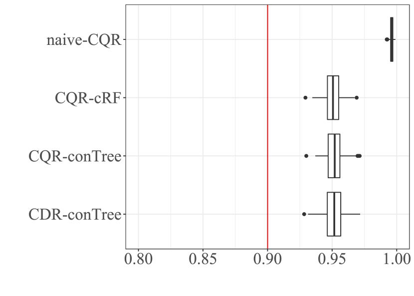
(a)

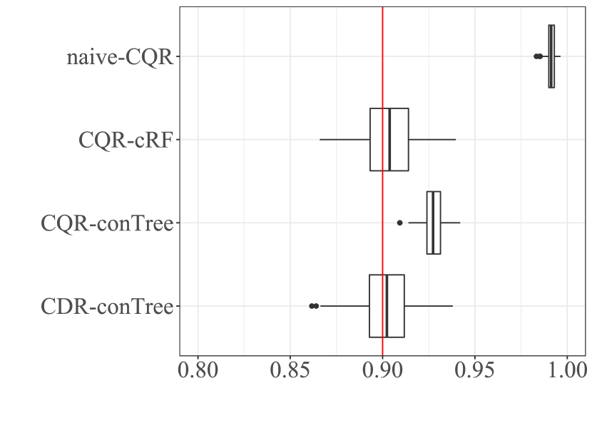
(b)

Figure 8: Empirical $90\%$ coverage of (a) the uncensored survival time $T$ and (b) the partially censored survival time $C_{\mathrm{loss}}\wedge T$. The abbreviations are the same as in Figure 1.

.

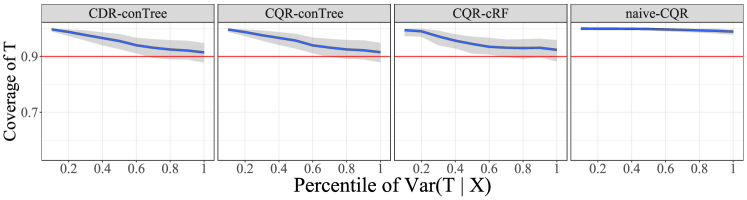
(a)

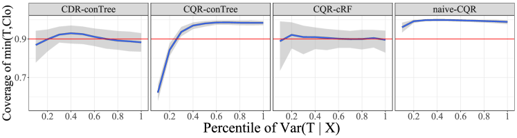
(b) .

Figure 9: Empirical $90\%$ conditional coverage of (a) the uncensored survival time $T$ and (b) the paritally censored survival time $T\wedge C_{\mathrm{loss}}$ as functions of $\mathrm{Var}(T\mid X)$. The other details are the same as in Figure 2.

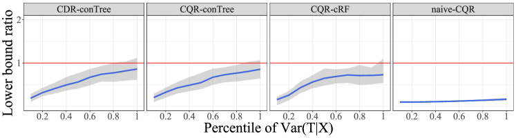
Figure 10: Ratio between the LPB and the theoretical quantile as a function of $\mathrm{Var}(T\mid X)$. The other details are the same as in Figure 2.

.

References

- Aitchison and Dunsmore (1980) Aitchison, J. and Dunsmore, I. R. (1980) Statistical prediction analysis. CUP Archive.
- Allison (1984) Allison, P. D. (1984) Event history analysis: Regression for longitudinal event data. No. 46. Sage.
- Anisimov and Fedorov (2007) Anisimov, V. V. and Fedorov, V. V. (2007) Modelling, prediction and adaptive adjustment of recruitment in multicentre trials. Statistics in medicine, 26, 4958–4975.
- Athey et al. (2019) Athey, S., Tibshirani, J. and Wager, S. (2019) Generalized random forests. The Annals of Statistics, 47, 1148–1178.
- von Bahr and Esseen (1965) von Bahr, B. and Esseen, C.-G. (1965) Inequalities for the -th absolute moment of a sum of random variables, . The Annals of Mathematical Statistics, 36, 299–303.
- Bain (2017) Bain, L. (2017) Statistical analysis of reliability and life-testing models: theory and methods. Routledge.
- Barber et al. (2019a) Barber, R. F., Candès, E. J., Ramdas, A. and Tibshirani, R. J. (2019a) The limits of distribution-free conditional predictive inference. Information and Inference: A Journal of the IMA.
- Barber et al. (2019b) Barber, R. F., Candes, E. J., Ramdas, A. and Tibshirani, R. J. (2019b) Predictive inference with the Jackknife+. arXiv preprint arXiv:1905.02928.
- Barnard et al. (2010) Barnard, K. D., Dent, L. and Cook, A. (2010) A systematic review of models to predict recruitment to multicentre clinical trials. BMC medical research methodology, 10, 1–8.
- Breslow (1975) Breslow, N. E. (1975) Analysis of survival data under the proportional hazards model. International Statistical Review/Revue Internationale de Statistique, 45–57.
- Bycroft et al. (2018) Bycroft, C., Freeman, C., Petkova, D., Band, G., Elliott, L. T., Sharp, K., Motyer, A., Vukcevic, D., Delaneau, O., O’Connell, J. et al. (2018) The UK Biobank resource with deep phenotyping and genomic data. Nature, 562, 203–209.
- Carter (2004) Carter, R. E. (2004) Application of stochastic processes to participant recruitment in clinical trials. Controlled clinical trials, 25, 429–436.
- Carter et al. (2005) Carter, R. E., Sonne, S. C. and Brady, K. T. (2005) Practical considerations for estimating clinical trial accrual periods: application to a multi-center effectiveness study. BMC medical research methodology, 5, 1–5.
- Cauchois et al. (2020) Cauchois, M., Gupta, S. and Duchi, J. (2020) Knowing what you know: valid confidence sets in multiclass and multilabel prediction. arXiv preprint arXiv:2004.10181.
- Chernozhukov et al. (2019) Chernozhukov, V., Wüthrich, K. and Zhu, Y. (2019) Distributional conformal prediction. arXiv preprint arXiv:1909.07889.
- Cox (1972) Cox, D. R. (1972) Regression models and life-tables. Journal of the Royal Statistical Society: Series B (Methodological), 34, 187–202.
- D’Amour et al. (2021) D’Amour, A., Ding, P., Feller, A., Lei, L. and Sekhon, J. (2021) Overlap in observational studies with high-dimensional covariates. Journal of Econometrics, 221, 644–654.
- Efron (1979) Efron, B. (1979) Bootstrap methods: Another look at the Jackknife. The Annals of Statistics, 1–26.
- Efron (2020) — (2020) Prediction, estimation, and attribution. International Statistical Review, 88, S28–S59.
- Efron and Tibshirani (1994) Efron, B. and Tibshirani, R. J. (1994) An introduction to the bootstrap. CRC press.
- Emanuel et al. (2020) Emanuel, E., Persad, G., Upshur, R., Thome, B., Parker, M., Glickman, A., Zhang, C., Boyle, C., Smith, M. and Phillips, J. (2020) Fair allocation of scarce medical resources in the time of Covid-19. The New England Journal of Medicine, 382.
- Faraggi and Simon (1995) Faraggi, D. and Simon, R. (1995) A neural network model for survival data. Statistics in medicine, 14, 73–82.
- Friedman and Narasimhan (2020) Friedman, J. and Narasimhan, B. (2020) conTree: Contrast Trees and Boosting. URL: https://jhfhub.github.io/conTree_tutorial. R package version 0.2-8.
- Friedman (2020) Friedman, J. H. (2020) Contrast trees and distribution boosting. Proceedings of the National Academy of Sciences, 117, 21175–21184.
- Gajewski et al. (2008) Gajewski, B. J., Simon, S. D. and Carlson, S. E. (2008) Predicting accrual in clinical trials with bayesian posterior predictive distributions. Statistics in medicine, 27, 2328–2340.
- Geisser (1993) Geisser, S. (1993) Predictive inference, vol. 55. CRC press.
- Goeman (2010) Goeman, J. J. (2010) L1 penalized estimation in the Cox proportional hazards model. Biometrical journal, 52, 70–84.
- Guan (2019) Guan, L. (2019) Conformal prediction with localization. arXiv preprint arXiv:1908.08558.
- Gui and Li (2005) Gui, J. and Li, H. (2005) Penalized Cox regression analysis in the high-dimensional and low-sample size settings, with applications to microarray gene expression data. Bioinformatics, 21, 3001–3008.
- Gupta et al. (2019) Gupta, C., Kuchibhotla, A. K. and Ramdas, A. K. (2019) Nested conformal prediction and quantile out-of-bag ensemble methods. arXiv preprint arXiv:1910.10562.
- Harrell Jr (2015) Harrell Jr, F. E. (2015) Regression modeling strategies: with applications to linear models, logistic and ordinal regression, and survival analysis. Springer.
- Hong and Tamer (2003) Hong, H. and Tamer, E. (2003) Inference in censored models with endogenous regressors. Econometrica, 71, 905–932.
- Hothorn et al. (2006) Hothorn, T., Bühlmann, P., Dudoit, S., Molinaro, A. and Van Der Laan, M. J. (2006) Survival ensembles. Biostatistics, 7, 355–373.
- Ishwaran et al. (2008) Ishwaran, H., Kogalur, U. B., Blackstone, E. H., Lauer, M. S. et al. (2008) Random survival forests. Annals of Applied Statistics, 2, 841–860.
- Kalbfleisch and Prentice (2011) Kalbfleisch, J. D. and Prentice, R. L. (2011) The statistical analysis of failure time data, vol. 360. John Wiley & Sons.
- Kaplan and Meier (1958) Kaplan, E. L. and Meier, P. (1958) Nonparametric estimation from incomplete observations. Journal of the American statistical association, 53, 457–481.
- Katzman et al. (2016) Katzman, J. L., Shaham, U., Cloninger, A., Bates, J., Jiang, T. and Kluger, Y. (2016) Deep survival: A deep Cox proportional hazards network. stat, 1050.
- Koenker (2020) Koenker, R. (2020) quantreg: Quantile Regression. URL: https://CRAN.R-project.org/package=quantreg. R package version 5.75.
- Korn (1986) Korn, E. L. (1986) Censoring distributions as a measure of follow-up in survival analysis. Statistics in medicine, 5, 255–260.
- Krishnamoorthy and Mathew (2009) Krishnamoorthy, K. and Mathew, T. (2009) Statistical tolerance regions: theory, applications, and computation, vol. 744. John Wiley & Sons.
- Lagakos (1979) Lagakos, S. W. (1979) General right censoring and its impact on the analysis of survival data. Biometrics, 139–156.
- Lao et al. (2017) Lao, J., Chen, Y., Li, Z.-C., Li, Q., Zhang, J., Liu, J. and Zhai, G. (2017) A deep learning-based radiomics model for prediction of survival in glioblastoma multiforme. Scientific reports, 7, 1–8.
- Lei et al. (2018) Lei, J., G’Sell, M., Rinaldo, A., Tibshirani, R. J. and Wasserman, L. (2018) Distribution-free predictive inference for regression. Journal of the American Statistical Association, 113, 1094–1111.
- Lei et al. (2013) Lei, J., Robins, J. and Wasserman, L. (2013) Distribution-free prediction sets. Journal of the American Statistical Association, 108, 278–287.
- Lei and Wasserman (2014) Lei, J. and Wasserman, L. (2014) Distribution-free prediction bands for non-parametric regression. Journal of the Royal Statistical Society: Series B: Statistical Methodology, 71–96.
- Lei and Candès (2021) Lei, L. and Candès, E. J. (2021) Conformal inference of counterfactuals and individual treatment effects. Journal of the Royal Statistical Society: Series B (Statistical Methodology).
- Leung et al. (1997) Leung, K.-M., Elashoff, R. M. and Afifi, A. A. (1997) Censoring issues in survival analysis. Annual review of public health, 18, 83–104.
- Li and Bradic (2020) Li, A. H. and Bradic, J. (2020) Censored quantile regression forest. In International Conference on Artificial Intelligence and Statistics, 2109–2119. PMLR.
- Murphy et al. (1997) Murphy, S., Rossini, A. and van der Vaart, A. W. (1997) Maximum likelihood estimation in the proportional odds model. Journal of the American Statistical Association, 92, 968–976.
- Neyman (1923/1990) Neyman, J. (1923/1990) On the application of probability theory to agricultural experiments. Essay on principles. Section 9. Statistical Science, 5, 465–472. Translated and edited by D. M. Dabrowska and T. P. Speed from the Polish original, which appeared in Roczniki Nauk Rolniczyc, Tom X (1923): 1–51 (Annals of Agricultural Sciences).
- Peng and Huang (2008) Peng, L. and Huang, Y. (2008) Survival analysis with quantile regression models. Journal of the American Statistical Association, 103, 637–649.
- Portnoy (2003) Portnoy, S. (2003) Censored regression quantiles. Journal of the American Statistical Association, 98, 1001–1012.
- Powell (1986) Powell, J. L. (1986) Censored regression quantiles. Journal of econometrics, 32, 143–155.
- Ranney et al. (2020) Ranney, M. L., Griffeth, V. and Jha, A. K. (2020) Critical supply shortages—the need for ventilators and personal protective equipment during the Covid-19 pandemic. New England Journal of Medicine, 382, e41.
- Ratkovic and Tingley (2021) Ratkovic, M. and Tingley, D. (2021) Estimation and inference on nonlinear and heterogeneous effects. Tech. rep. URL: https://scholar.harvard.edu/files/dtingley/files/mdei.pdf.
- Romano et al. (2019a) Romano, Y., Barber, R. F., Sabatti, C. and Candès, E. J. (2019a) With malice towards none: Assessing uncertainty via equalized coverage. arXiv preprint arXiv:1908.05428.
- Romano et al. (2019b) Romano, Y., Patterson, E. and Candes, E. (2019b) Conformalized quantile regression. In Advances in Neural Information Processing Systems, 3543–3553.
- Romano et al. (2020) Romano, Y., Sesia, M. and Candès, E. J. (2020) Classification with valid and adaptive coverage. arXiv preprint arXiv:2006.02544.
- Rosenbaum and Rubin (1983) Rosenbaum, P. R. and Rubin, D. B. (1983) The central role of the propensity score in observational studies for causal effects. Biometrika, 70, 41–55.
- Rosenthal (1970) Rosenthal, H. P. (1970) On the subspaces of spanned by sequences of independent random variables. Israel Journal of Mathematics, 8, 273–303.
- Rubin (1974) Rubin, D. B. (1974) Estimating causal effects of treatments in randomized and nonrandomized studies. Journal of educational Psychology, 66, 688.
- Rubin (1978) — (1978) Bayesian inference for causal effects: The role of randomization. The Annals of statistics, 34–58.
- Sadinle et al. (2019) Sadinle, M., Lei, J. and Wasserman, L. (2019) Least ambiguous set-valued classifiers with bounded error levels. Journal of the American Statistical Association, 114, 223–234.
- Sant’Anna (2016) Sant’Anna, P. H. (2016) Program evaluation with right-censored data. arXiv preprint arXiv:1604.02642.
- Saunders et al. (1999) Saunders, C., Gammerman, A. and Vovk, V. (1999) Transduction with confidence and credibility. In Proceedings of the Sixteenth International Joint Conference on Artificial Intelligence, 722–726.
- Scharfstein and Robins (2002) Scharfstein, D. O. and Robins, J. M. (2002) Estimation of the failure time distribution in the presence of informative censoring. Biometrika, 89, 617–634.
- Schemper and Smith (1996) Schemper, M. and Smith, T. L. (1996) A note on quantifying follow-up in studies of failure time. Controlled clinical trials, 17, 343–346.
- Sesia and Candès (2020) Sesia, M. and Candès, E. J. (2020) A comparison of some conformal quantile regression methods. Stat, 9, e261.
- Shafer and Vovk (2008) Shafer, G. and Vovk, V. (2008) A tutorial on conformal prediction. Journal of Machine Learning Research, 9, 371–421.
- Shah et al. (2020) Shah, R. D., Peters, J. et al. (2020) The hardness of conditional independence testing and the generalised covariance measure. Annals of Statistics, 48, 1514–1538.
- Simon et al. (2011) Simon, N., Friedman, J., Hastie, T. and Tibshirani, R. (2011) Regularization paths for Cox’s proportional hazards model via coordinate descent. Journal of statistical software, 39, 1.
- Stine (1985) Stine, R. A. (1985) Bootstrap prediction intervals for regression. Journal of the American Statistical Association, 80, 1026–1031.
- Therneau (2020) Therneau, T. M. (2020) A Package for Survival Analysis in R. URL: https://CRAN.R-project.org/package=survival. R package version 3.2-7.
- Tibshirani (1997) Tibshirani, R. (1997) The lasso method for variable selection in the Cox model. Statistics in medicine, 16, 385–395.
- Tibshirani et al. (2019) Tibshirani, R. J., Foygel Barber, R., Candes, E. and Ramdas, A. (2019) Conformal prediction under covariate shift. Advances in Neural Information Processing Systems, 32, 2530–2540.
- Tsybakov (2008) Tsybakov, A. B. (2008) Introduction to nonparametric estimation. Springer Science & Business Media.
- Vergano et al. (2020) Vergano, M., Bertolini, G., Giannini, A., Gristina, G., Livigni, S., Mistraletti, G., Riccioni, L. and Petrini, F. (2020) Clinical ethics recommendations for the allocation of intensive care treatments in exceptional, resource-limited circumstances: the italian perspective during the COVID-19 epidemic. Critical Care, 24.
- Vershynin (2018) Vershynin, R. (2018) High-dimensional probability: An introduction with applications in data science, vol. 47. Cambridge university press.
- Verweij and Van Houwelingen (1993) Verweij, P. J. and Van Houwelingen, H. C. (1993) Cross-validation in survival analysis. Statistics in medicine, 12, 2305–2314.
- Vovk (2002) Vovk, V. (2002) On-line confidence machines are well-calibrated. In The 43rd Annual IEEE Symposium on Foundations of Computer Science, 2002. Proceedings., 187–196. IEEE.
- Vovk (2012) — (2012) Conditional validity of inductive conformal predictors. In Asian conference on machine learning, 475–490.
- Vovk et al. (2005) Vovk, V., Gammerman, A. and Shafer, G. (2005) Algorithmic learning in a random world. Springer Science & Business Media.
- Vovk et al. (2003) Vovk, V., Lindsay, D., Nouretdinov, I. and Gammerman, A. (2003) Mondrian confidence machine. Technical Report.
- Wald (1943) Wald, A. (1943) An extension of wilks’ method for setting tolerance limits. The Annals of Mathematical Statistics, 14, 45–55.
- Wang et al. (2019) Wang, P., Li, Y. and Reddy, C. K. (2019) Machine learning for survival analysis: A survey. ACM Computing Surveys (CSUR), 51, 1–36.
- Wei (1992) Wei, L.-J. (1992) The accelerated failure time model: a useful alternative to the Cox regression model in survival analysis. Statistics in medicine, 11, 1871–1879.
- Wilks (1941) Wilks, S. S. (1941) Determination of sample sizes for setting tolerance limits. The Annals of Mathematical Statistics, 12, 91–96.
- Witten and Tibshirani (2010) Witten, D. M. and Tibshirani, R. (2010) Survival analysis with high-dimensional covariates. Statistical methods in medical research, 19, 29–51.
- Wu and Carroll (1988) Wu, M. C. and Carroll, R. J. (1988) Estimation and comparison of changes in the presence of informative right censoring by modeling the censoring process. Biometrics, 175–188.
- Yang and Kuchibhotla (2021) Yang, Y. and Kuchibhotla, A. K. (2021) Finite-sample efficient conformal prediction. arXiv preprint arXiv:2104.13871.
- Zhang and Lu (2007) Zhang, H. H. and Lu, W. (2007) Adaptive lasso for Cox’s proportional hazards model. Biometrika, 94, 691–703.