Diversified Multiscale Graph Learning with Graph Self-Correction

Abstract

Though the multiscale graph learning techniques have enabled advanced feature extraction frameworks, the classic ensemble strategy may show inferior performance while encountering the high homogeneity of the learnt representation, which is caused by the nature of existing graph pooling methods. To cope with this issue, we propose a diversified multiscale graph learning model equipped with two core ingredients: a graph self-correction (GSC) mechanism to generate informative embedded graphs, and a diversity boosting regularizer (DBR) to achieve a comprehensive characterization of the input graph. The proposed GSC mechanism compensates the pooled graph with the lost information during the graph pooling process by feeding back the estimated residual graph, which serves as a plug-in component for popular graph pooling methods. Meanwhile, pooling methods enhanced with the GSC procedure encourage the discrepancy of node embeddings, and thus it contributes to the success of ensemble learning strategy. The proposed DBR instead enhances the ensemble diversity at the graph-level embeddings by leveraging the interaction among individual classifiers. Extensive experiments on popular graph classification benchmarks show that the proposed GSC mechanism leads to significant improvements over state-of-the-art graph pooling methods. Moreover, the ensemble multiscale graph learning models achieve superior enhancement by combining both GSC and DBR.

1 Introduction

Graph Neural Networks (GNNs) have been developed rapidly for modeling graph-structured data and achieved remarkable progress in graph representation learning as well as downstream learning tasks, such as bioinformatics and social networks analysis [18, 10, 41, 37]. While many GNNs learn graph representation at a fixed scale, the multiscale graph learning has also attracted a surge of interests [4, 27, 7, 9, 21, 25], for its capability of capturing both fine and coarse graph structures and features (representing local and global information, respectively). Several advanced feature extraction frameworks have been proposed for multiscale graph learning. Some attempts adopt the encoder-decoder pipeline to embed the input-graph and perform feature updating in the latent coarsest graph [4, 27, 7]. Other works utilize the pyramid architecture to extract multiscale graph features, and perform feature aggregation via skip-connection [9, 21], or cross-layer summation fusion [25].

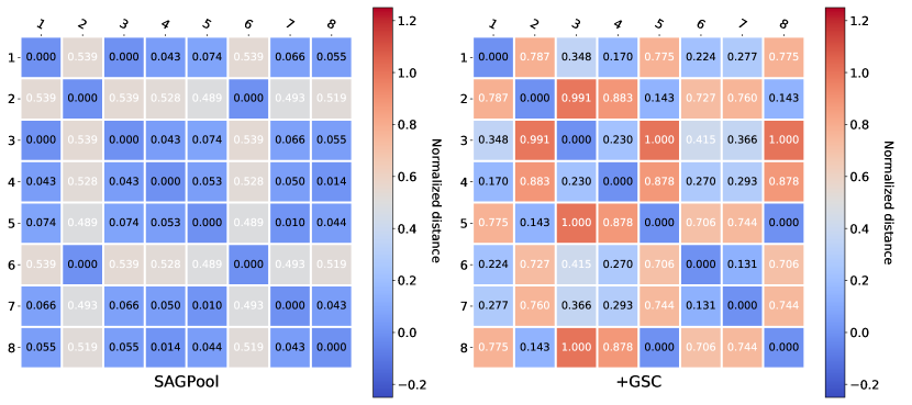
Figure 1: Distance heatmap of node features of the last graph pooling layers. Node features become highly homogenized in SAGPool [21] (left), while graph self-correction well preserves node discrepancy (right) from the initial features (see Figure 4).

Orthogonal to various multiscale feature learning techniques, one straightforward and promising strategy for adequately leveraging the extracted graph embeddings is to construct ensembles of multiple individual classifiers in a stacking style, where each classifier receives a graph embedding at a fixed granularity, and predicted logits of all classifiers are then averaged to produce the final prediction. As a generic method, such ensemble models are expected to obtain more reliable predictions. Meanwhile, the success of ensemble learning crucially depends on two properties of each individual classifier: high accuracy and high diversity [8, 34]. The first property is readily satisfied due to the high expressive power of deep neural networks [5], however, the second one may not hold in the scenario of multiscale graph learning.

Table 1: The failing of the simple ensemble strategy (denoted with ‘+’) on enhancing multiscale GNNs. Detail settings are stated in Section 6. More verifications are given in Appendix.

Method	PROTEINS	NCI1	NCI109
SAGPool	73.26±0.78 (-)	69.88±0.82 (-)	70.07±0.69 (-)
SAGPool+	72.56±0.76 ($\downarrow$)	69.61±0.62 ($\downarrow$)	69.41±0.66 ($\downarrow$)
ASAP	74.14±0.33 (-)	74.27±0.63 (-)	72.90±0.59 (-)
ASAP+	74.21±0.69 ($\uparrow$)	73.62±0.56 ($\downarrow$)	72.52±0.45 ($\downarrow$)

As indicated in recent researches [30, 1], the indispensable graph pooling operation for establishing multiscale graph learning may have led to the high homogeneity of the node embeddings. Mesquita et al. [30] observe that graph pooling via the learnable cluster assignment procedure [42, 17, 1] exacerbate the homogeneity of node embeddings, and thus a comparable performance could be obtained by just replacing the complicated assignment matrix with some random matrix. Bianchi et al. [1] notice a similar issue in graph pooling methods based on the Top-K vertex selection mechanism [9, 21]. That is, these pooling layers would tend to select nodes that are highly-connected and share similar features. Due to the homogeneity of the node embeddings, the generated graph embeddings at various granularity tend to become homogeneous as well. Under this circumstance, these homogeneous graph embeddings lead to limited diversity among learned classifiers. Since diversity is crucial for the success of ensemble methods, it is probable that the ensemble strategy will fail in boosting the performance of multiscale GNNs equipped with these pooling modules, or even become detrimental to them. This is verified by the experiments results given in Table 1.

A common solution to improve the ensemble diversity is to build multiple classifiers that get trained with different sampled data in an independent manner. Nevertheless, it requires much more expensive computational cost and ignores the interaction among individual classifiers, which might also lead to shared feature representations among these members and would not be helpful to improve the performance [19]. To address the issues discussed above, we design a diversified multiscale graph learning model that includes two main technical contributions: 1) a graph self-correction mechanism to generate informative pooled graphs, which also hampers the homogeneity of node embeddings and thus promotes the ensemble diversity at the node-level embeddings, and 2) a diversity boosting regularizer to directly model and optimize the ensemble diversity at the graph-level embeddings.

The graph self-correction mechanism. It is intuitive to attribute the homogenization of node embeddings to the information loss caused by graph pooling operations. Existing pooling methods mainly focus on how to construct the structure of the coarsened graph [42, 17, 1, 9, 21, 14, 23], either through a cluster assignment procedure or a Top-K vertex selection mechanism. However, few works have studied how to generate high-quality coarsened graphs with adequate semantic information. We aim in this target by introducing Graph Self-Correcting (GSC) mechanism to compensate for the information loss during the graph pooling process. As we will show, GSC works by moving the emphasis of the graph pooling problem from direct learning an embedded pooled graph to a two-stage target: first, searching the optimal pooled graph structure, and second, self-correcting the semantic embeddings of it. Notably, GSC not only enhances the embedding quality of the pooled graph by serving as a plug-and-play method, but also relieves the homogeneity of node features (as shown in Figure 1), which further contributes to the success of the ensemble strategy on the multiscale graph learning model.

The diversity boosting regularizer.

Another key ingredient of our contributions is to directly emphasize the diversity among the graph embeddings at different granularity. It’s also expected to provide a comprehensive characterization of the input graph from multiple diversified graph embeddings. Specifically, we leverage the interaction among base learners and model the ensemble diversity on the graph embeddings of each scaled graph. Under this definition, we propose a diversity boosting regularizer (DBR) to further diversify the multiscale graph learning model. Note that previous work has devised ensemble diversity on the level of model predictions [16, 32, 44], and we also make a discussion with them.

To validate the effectiveness of our methods, we conduct extensive experiments on popular graph classification benchmark datasets to perform a comparative study. We show that our GSC leads to significant improvements over state-of-the-art graph pooling methods. Meanwhile, combing both GSC and DBR can consistently boost the ensemble multiscale graph learning model.

2 Related Work

2.1 Graph Pooling Modules

For extracting multiple graphs at different scales, the graph pooling operation is essential to downsample the input full-graph. Since the graphs are often irregular data which lies on the non-Euclidean domain, the locality of them is not well-defined. And hence, mature pooling techniques in Convolutional Neural Networks (CNNs) devised for processing regular data, such as image, can not be naturally extended to GNNs. In some early attempts, researchers adopt some deterministic and heuristic methods to perform graph pooling. Either applying global pooling over all node embeddings [12] or coarsening the graph via traditional cluster assignment algorithms [2, 6] are included in this aspect. Further works focus on establishing the end-to-end hierarchical learning manner for embedding the graph The first research line is distributed to turning the problem of graph pooling into vertex clustering through parameterizing the cluster assignment procedure so that the differentiable pooling operator is built. DiffPool [42] leverages the node features and graph topology to learn the soft assignment matrix for the first time. MinCUT [1] proposes a relaxed formulation of the spectral clustering and improve the DiffPool to some extent. GMN [17] generates the assignment matrix using a sequence of memory layers. Additionally, HaarPool [29] and EigenPool [39] are spectral-based pooling methods that use the spectral clustering to generate the coarsened graphs, but their time complexity costs are relatively higher. Another technical line is based on the Top-K vertex selection mechanism, which introduces a scorer model to calculate the importance score of each node, and the nodes with K highest scores are retained to construct the coarsened graph. gPool [9] firstly uses the node features to train the scorer model, and SAGPool [21] improves upon it by further leveraging the graph topology for scoring nodes. AttPool [14] proposes a similar scoring model as SAGPool and a local-attention mechanism to prevent the sampled nodes from stucking in certain region. ASAP [33] proposes to update the nodes in the same cluster via a self-attention mechanism, and then scoring the nodes based on such enhanced node features. It also updates the adjacency matrix following DiffPool to maintain graph connectivity. The Top-$K$ vertex selection based methods are usually more efficient since it avoids learning the dense assignment matrix.

2.2 Feedback Networks

Feedback networks decompose a one-step prediction procedure into multiple steps for establishing a mechanism of perceiving errors and making corrections. It has been used in many visual tasks [3, 11, 24, 28, 35, 36]. For the case of human pose estimation [3], the feedback network iteratively estimates the position deviation and applies it back to the current estimation. DBPN [11] proposes a projection module to involve iterative up- and down-sampling process in the super-resolution network. To our knowledge, the notion of feedback procedures has not been applied to GNNs, especially the graph pooling operation. This extension is technically non-trivial. While the offset or distortion produced in the prediction is clear for image signals, the irregular structures of graphs make identifying what is missing or undesirable a challenge. In this paper, we devise two schemes of graph self-correction and obtain considerable performance improvement, though we do not adopt an iterative process for the consideration of computational cost.

3 Preliminaries

Throughout this work, a graph is represented as $\mathcal{G}(\mathcal{V},\mathbf{A})$, where $\mathcal{V}$ is vertex set that has $N$ nodes with $d_{0}$-dimension features of $\mathbf{X}\in\mathbb{R}^{N\times d_{0}}$, and $\mathbf{A}\in\mathbb{R}^{N\times N}$ is the adjacency matrix. Note that we omit the edge features in this paper for simplicity. The node degree matrix is given by $\mathbf{D}=\mathrm{diag}(\mathbf{A}\mathbf{1}_{N})$. The adjacency matrix with inserted self-loops is $\hat{\mathbf{A}}=\mathbf{A}+\mathbf{I}$, and the corresponding degree matrix is denoted as $\hat{\mathbf{D}}$. Given a node $v$, its connected-neighbors are denoted as $\mathcal{N}_{v}$. For a matrix $\mathbf{X}$, $\mathbf{X}_{i,:}$ denotes its $i$-th row and $\mathbf{X}_{:,j}$ denotes its $j$-th column.

3.1 Multiscale Graph Neural Networks

The key operation of GNNs can be abstracted to a process that involves message passing among the nodes in the graph. The message passing operation iteratively updates a node $v$’s hidden states, $\mathbf{X}_{v,:}\in\mathbb{R}^{1\times d}$, by aggregating the hidden states of $v$’s neighboring nodes. In general, the message passing process involves several iterations, each one can be formulated as,

$$\mathbf{m}_{v}^{{(l)}}=\mathrm{AGGR}^{(l)}(\{(\mathbf{X}_{v,:}^{(l-1)},\mathbf{X}_{u,:}^{(l-1)})\;|\;u\in\mathcal{N}_{v}\}),$$

$$\mathbf{X}_{v,:}^{(l)}=\sigma(\mathbf{W}^{(l)}\mathbf{m}_{v}^{{(l)}}+\mathbf{b}^{(l)}),$$ (1)

where $\mathrm{AGGR}^{(l)}(\cdot)$ is the aggregation operator, $\mathbf{m}_{v}^{{(l)}}$ is the aggregated message, $\sigma(\cdot)$ is some activation function and $\mathbf{W}$, $\mathbf{b}$ are the trainable parameters. Usually we set the initial hidden states $\mathbf{X}^{(0)}$ as node ego-features $\mathbf{X}$.

Multiscale GNNs iteratively generate coarsened graphs to extract hierarchical representations, which are imperative for capturing both fine and coarse structural and semantic information, by repeating hierarchical graph pooling operations. Formally, assume there are $l_{t}$ number of message passing operations between $\mathrm{Pool}$ operation $P_{t-1}$ and $P_{t}$, i.e., the $t$-th $\mathrm{Pool}$ operation is acting on the $l_{t}$-th iterations of message passing on each scale’s graph,

$$\mathbf{X}^{{(0,P_{t})}},\mathbf{A}^{{(0,P_{t})}}=\mathrm{Pool}^{(t)}(\mathbf{X}^{{(l_{t-1},P_{t-1})}},\mathbf{A}^{{(l_{t-1},P_{t-1})}}),$$ (2)

where $t\in[1,T]$ represents the index number of the graph pooling layers. We make a convention that $\mathbf{X}^{{(l,P_{0})}}:=\mathbf{X}^{{(l)}}$ is the node feature matrix that has yet been pooled, and $\mathbf{X}^{{(0,P_{t+1})}}:=\mathbf{X}^{{(P_{t+1})}}$. Multiscale GNNs [7, 21, 25] utilize pooled graphs at multiple scales to perform feature fusion and generate final graph embedding,

$$\mathbf{x}_{G}=\mathrm{READOUT}(f(\{\mathbf{X}^{{(P_{0})}},...,\mathbf{X}^{{(P_{T})}}\})),$$ (3)

where the fusion function $f(\cdot)$, such as skip-connection [9, 21] or cross-scale summation [25], is used to aggregate multiscale graphs. The following $\mathrm{READOUT}$ is a permutation-invariant operator to get graph-level embeddings. Lastly, a classifier such as the multi-layer perceptron $\mathrm{MLP}$ is used to predict the category logits $\tilde{y}=\mathrm{MLP}(\mathbf{x}_{G})$.

4 Graph Self-Correction Mechanism

Existing graph pooling methods haven’t yet focused on generating high-quality coarsened graphs with rich semantic information, and the information loss caused by pooling operations may have caused the homogenization of representations. A core idea of Graph Self-Correction (GSC) mechanism is to reduce such information loss through compensating information generated by the feedback procedures. It contains three phases: graph pooling, compensated information calculation and information feedback.

4.1 Phase 1: Graph pooling

In the settings of GSC, the initial graph pooling layer concentrates on searching for the optimal structure of the coarsened graphs rather than directly learning both the topological and informative embeddings. As a preliminary step of the approach, it can be implemented by any kind of existing pooling methods [42, 1, 9, 21, 14, 33]. For the compactness of this paper, we only take the Top-$K$ vertex selection based pooling methods as the running example and we discuss the application of GSC on cluster assignment based methods in Appendix.

As a case of Eq.(2), SAGPool [21] adopts a $1$-layer GCN [18] as the node scorer, and uses the Top-$K$ selection strategy to select nodes retained in the coarsened graph,

$$\mathbf{s}^{{(t)}} =\sigma(\hat{\mathbf{D}}^{-\frac{1}{2}}\hat{\mathbf{A}}^{{(l_{t},P_{t})}}\hat{\mathbf{D}}^{-\frac{1}{2}}\mathbf{X}^{{(l_{t},P_{t})}}\mathbf{W}^{{(l_{t})}}),$$ (4)

$$\text{Idx}^{{(t)}} =\mathrm{Top}\text{-}\mathrm{K}(\mathbf{s}^{{(t)}},K),$$ (5)

where the $\mathrm{Top}$-$\mathrm{K}$ function returns the $K$ indices of the selected nodes based on the ranking order of $\mathbf{s}^{{(t)}}$, which are then used to pool down the input-graph as:

$$\mathbf{X}^{{(P_{t+1})}} =\mathbf{X}^{{(l_{t},P_{t})}}_{\text{Idx},:}\odot\mathbf{s}_{\text{Idx}},$$ (6)

$$\mathbf{A}^{{(P_{t+1})}} =\mathbf{A}^{{(l_{t},P_{t})}}_{\text{Idx},\text{Idx}},$$ (7)

where $\odot$ is the element-wise product to apply node scores as attention weights for updating the pooled node features.

4.2 Phase 2: Compensated information calculation

As noticed in the pooling process given by SAGPool, the subsequent pooled node features discard all information preserved in those unselected nodes, which might hurt the exploitation of rich semantic features in original graphs. Inspired by the feedback networks [3, 11, 24], GSC introduces a residual estimation procedure to calculate compensated information that empowers the self-correction of the embedded coarsened graph in the feedback stage. Specifically, we propose two schemes to calculate such residual signals: complement graph fusion and coarsened graph back-projection.

Complement graph fusion The graph composited by the unselected nodes after the graph pooling layer and their adjacency relations is defined as the complement of the pooled graph here. Then the indices of nodes in the complement graph formulate:

$$\text{CompIdx}=\{i(v)|v\in\mathcal{V}\;\text{and}\;i(v)\not\in\text{Idx}^{{(t)}}\},$$ (8)

where $i(\cdot)$ gives a unique index to a node. The complement denotes the information that has been lost during the first phase of GSC, and it can be adopted as the residual signal to be fused with the pooled graph. The approach is to propagate node features from the complement graph to the pooled graph leveraging an $\mathrm{UnPool}$ layer:

$$\mathbf{E}_{\text{Comp}}^{{(t)}}=\text{UnPool}(\mathbf{X}_{\text{Comp}}^{{(t)}},\mathbf{A}^{{(l_{t},P_{t})}}).$$ (9)

Here the $\mathrm{UnPool}$ denotes an unpooling process. It receives node features of the complement graph as the input feature and the original graph structure as adjacency relation, and interpolates compensated information to those selected nodes of the pooled graph. Similar to [9], it can be devised by initializing the input feature matrix $\mathbf{X}_{\text{Comp}}^{{(t)}}\in\mathbb{R}^{N\times d}$ as:

$$\mathbf{X}_{\text{Comp}}^{{(t)}}\text{[}i(v),:\text{]}=\begin{cases}\mathbf{X}_{i(v),:}^{{(l_{t},P_{t})}}&i(v)\in\text{CompIdx}\\ \mathbf{0}&\text{otherwise},\end{cases}\vspace{-1mm}$$ (10)

here we denote the index selection operator in the brackets of the left-hand side for clarity, and then $\mathrm{UnPool}$ propagate it by the message passing process, which is implemented by a 1-layer graph convolution network (GCN) [18].

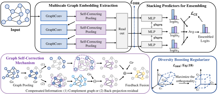
Figure 2: The ensembled multiscale graph learning framework (top), equipped with the proposed graph self-correction mechanism (bottom left) and diversity boosting regularizer (bottom right). The bottom-left module makes an illustration of the two modes of graph self-correction, and the bottom-right module provides a geometric interpretation of the regularizer.

Coarsened graph back-projection Another source of the compensated information is inspired by the classic back-projection algorithm [15] used for iteratively refining the restored high-resolution images. The intuition is that a pooled graph is ideal if it contains adequate information for reconstructing the original graph. Rather than introducing additional knowledge to model the pattern of lost information, coarsened graph back-projection manages to restore the original graph using the pooled node features themselves, and then calculates the reconstruction error to serve as the compensated signals. The restoration process is given by:

$$\mathbf{X}_{\text{Recon}}^{{(t)}}=\text{UnPool}(\mathbf{X}_{\text{Coarse}}^{{(t)}},\mathbf{A}^{{(l_{t},P_{t})}}),$$ (11)

where the input feature matrix of $\mathbf{X}_{\text{Coarse}}^{{(t)}}\in\mathbb{R}^{N\times d}$ is initialized by the pooled node features $\mathbf{X}^{{(P_{t+1})}}\in\mathbb{R}^{|\text{Idx}|\times d}$ with padding zero vectors:

$$\vspace{-1mm}\mathbf{X}_{\text{Coarse}}^{{(t)}}\text{[}i(v),:\text{]}=\begin{cases}\mathbf{X}_{i(v),:}^{{(t+1)}}&i(v)\in\text{Idx}\\ \mathbf{0}&\text{otherwise},\end{cases}$$ (12)

After that, the residual graph is calculated by:

$$\mathbf{E}_{\text{Recon}}^{{(t)}}=\mathbf{X}^{{(l_{t},P_{t})}}-\mathbf{X}_{\text{Recon}}^{{(t)}}.$$ (13)

4.3 Phase 3: Information feedback

GSC finally refines the pooled graph $\mathbf{X}^{{(P_{t+1})}}$ with the residual embedded graph of $\mathbf{E}^{{(l,P_{t})}}\in\mathbb{R}^{N\times d}$ as:

$$\tilde{\mathbf{X}}^{{(P_{t+1})}}=\mathbf{X}^{{(P_{t+1})}}+\mathbf{E}_{\text{Idx},:}^{{(t)}},\vspace{-1mm}$$ (14)

where $\mathbf{E}_{\text{Idx},:}^{{(t)}}\in\mathbb{R}^{|\text{Idx}|\times d}$ is tailored from the residual signal, either $\mathbf{E}_{\text{Comp}}^{{(t)}}\in\mathbb{R}^{N\times d}$ in Eq.(9), or $\mathbf{E}_{\text{Recon}}^{{(t)}}\in\mathbb{R}^{N\times d}$ in Eq.(13), using the indices $\text{Idx}^{{(t)}}$ given by Eq.(5).

The graph self-correction mechanism not only helps the feedback of information vanished in the pooling process, but also reduces the homogeneity among nodes, which indicates that the self-correction learns to preserve the discrepancy of the original graph. To verify this, we provide additional case studies and a deeper insight of the GSC mechanism in Section 6.3.1 for further discussion.

5 Diversified Multiscale Graph Learning

The graph self-correction mechanism proposed in Section 4 generates informative multiscale embedded graphs, which also encourages the discrepancy of node-level embeddings and thus contributes to the ensemble learning strategy. In this section, we first introduce the simple stacking-style ensemble multiscale graph learning model, and then propose the diversity boosting regularizer acting on the readout graph embeddings, which is working together with the GSC procedure to jointly enhance the diversity on node-level and graph-level representations.

Table 2: Performance comparison of GSC mechanism with other pooling methods. Methods with superscript ^∗ are the re-implemented version for a fair comparison. Methods denoted with ‘+’ are the ensembled models. Average accuracy and standard deviation are reported. Best result on each comparison is bolded. Best result of the non-ensembled models is underlined.

Dataset	D&D	PROTEINS	NCI1	NCI109	FRANKENSTEIN	OGB-MOLHIV
#Graphs	1178	1113	4110	4127	4337	41127
Avg #Nodes	284.3	39.1	29.9	29.7	16.9	25.5
Set2Set [38]	71.60 $\pm$ 0.87	72.16 $\pm$ 0.43	66.97 $\pm$ 0.74	61.04 $\pm$ 2.69	61.46 $\pm$ 0.47	–
GlobalAttention [26]	71.38 $\pm$ 0.78	71.87 $\pm$ 0.60	69.00 $\pm$ 0.49	67.87 $\pm$ 0.40	61.31 $\pm$ 0.41	–
SortPool [45]	71.87 $\pm$ 0.96	73.91 $\pm$ 0.72	68.74 $\pm$ 1.07	68.59 $\pm$ 0.67	63.44 $\pm$ 0.65	–
DiffPool [42]	66.95 $\pm$ 2.41	68.20 $\pm$ 2.02	62.23 $\pm$ 1.90	61.98 $\pm$ 1.98	60.60 $\pm$ 1.62	–
TopK [9]	75.01 $\pm$ 0.86	71.10 $\pm$ 0.90	67.02 $\pm$ 2.25	66.12 $\pm$ 1.60	61.46 $\pm$ 0.84	–
SAGPool∗ [21]	75.88 $\pm$ 0.72	73.26 $\pm$ 0.78	69.88 $\pm$ 0.82	70.07 $\pm$ 0.69	60.68 $\pm$ 0.49	73.16 $\pm$ 2.3
w/ GSC-B	76.03 $\pm$ 0.68 (-)	74.27 $\pm$ 0.80 (-)	71.91 $\pm$ 0.93 (-)	71.69 $\pm$ 0.70 (-)	61.85 $\pm$ 0.79 (-)	73.53 $\pm$ 2.6 (-)
w/ GSC-B+	76.49 $\pm$ 0.96 ($\uparrow$)	74.47 $\pm$ 0.72 ($\uparrow$)	73.10 $\pm$ 0.69 ($\uparrow$)	72.13 $\pm$ 0.69 ($\uparrow$)	62.54 $\pm$ 0.47 ($\uparrow$)	72.73 $\pm$ 2.1 ($\uparrow$)
w/ GSC-C	76.02 $\pm$ 0.67 (-)	74.36 $\pm$ 0.66 (-)	72.38 $\pm$ 0.69 (-)	72.03 $\pm$ 0.70 (-)	63.19 $\pm$ 0.62 (-)	73.87 $\pm$ 1.6 (-)
w/ GSC-C+	76.57 $\pm$ 1.04 ($\uparrow$)	74.89 $\pm$ 0.70 ($\uparrow$)	72.77 $\pm$ 0.73 ($\uparrow$)	72.76 $\pm$ 0.57 ($\uparrow$)	63.65 $\pm$ 0.54 ($\uparrow$)	74.01 $\pm$ 1.6 ($\uparrow$)
ASAP∗ [33]	76.77 $\pm$ 0.58	74.14 $\pm$ 0.33	74.27 $\pm$ 0.63	72.90 $\pm$ 0.59	64.58 $\pm$ 0.23	73.41 $\pm$ 2.2
w/ GSC-B	76.80 $\pm$ 0.54 (-)	74.39 $\pm$ 0.71 (-)	74.52 $\pm$ 0.69 (-)	$\underline{\text{73.64}}$ $\pm$ 0.49 (-)	64.34 $\pm$ 0.45 (-)	$\underline{\text{74.99}}$ $\pm$ 1.7 (-)
w/ GSC-B+	77.46 $\pm$ 0.60 ($\uparrow$)	74.86 $\pm$ 0.51 ($\uparrow$)	74.93 $\pm$ 0.67 ($\uparrow$)	74.32 $\pm$ 0.47 ($\uparrow$)	65.01 $\pm$ 0.65 ($\uparrow$)	75.31 $\pm$ 1.5 ($\uparrow$)
w/ GSC-C	$\underline{\text{77.30}}$ $\pm$ 0.72 (-)	$\underline{\text{74.77}}$ $\pm$ 0.49 (-)	$\underline{\text{74.83}}$ $\pm$ 0.41 (-)	73.37 $\pm$ 0.58 (-)	$\underline{\text{65.90}}$ $\pm$ 0.32 (-)	74.08 $\pm$ 1.8 (-)
w/ GSC-C+	77.35 $\pm$ 0.53 ($\uparrow$)	75.15 $\pm$ 0.60 ($\uparrow$)	74.84 $\pm$ 0.60 ($\uparrow$)	73.57 $\pm$ 0.45 ($\uparrow$)	66.17 $\pm$ 0.68 ($\uparrow$)	74.76 $\pm$ 1.4 ($\uparrow$)

5.1 Model Architecture

To fairly identify the contribution of each proposed ingredients, we design the multiscale graph learning framework following [9, 21, 33]. In that case, $T$ and $L$ both equal to $3$ and $l_{t}$ is fixed to $1$ across all pooling layers. The hierarchical pooled graphs at three scales are generated by three simple stacking modules of $\mathrm{GraphConv}$-$\mathrm{Pooling}$, then the graph embeddings are readout by the global pooling process separately. We follow previous works to use a 1-layer GCN [18] followed by an activation function to work as $\mathrm{GraphConv}$. $\mathrm{Pooling}$ consists of the baseline pooling module to be compared with and the proposed GSC mechanism. As a baseline backbone, the three graph embeddings are summed together before passing to an $\mathrm{MLP}$ to get the prediction logits. For clarity, we provide the schemata of this baseline backbone in Appendix.

For performing the ensembled prediction, we modify the prediction module with three parameter-shared $\mathrm{MLP}$s, and each one receives a graph embedding from fixed granularity for predicting individual logits. Here the $\mathrm{MLP}$-sharing setting is for conducting rigorous controlled experiments. After that, the ensembled logits are obtained by averaging three individual logits. The model is depicted in Figure 2. Noticed that the individual classifiers are a part of the multiscale learning architecture, thus they are trained on the same mini-batch of data but differ in the granularity of graphs to be readout as input. This feature enables us to utilize the interactions among these base learners and improves the training process, as stated in the below section.

5.2 Diversity Boosting Regularizers

The collection of multiscale graph embeddings formulates $\mathbf{G}=(\mathbf{x}_{G}^{{(P_{1})}},\cdot\cdot\cdot,\mathbf{x}_{G}^{{(P_{T})}})^{\mathrm{T}}\in\mathbb{R}^{T\times d}$, where each element $\mathbf{x}_{G}^{{(P_{t})}}\in\mathbb{R}^{1\times d}$ is readout from $\{\mathbf{X}_{v,:}^{{(P_{t})}}|v\in\mathcal{V}\}$ as a case of Eq.(3). Motivated by the theory of determinant point processes (DPPs) [20], we define the diversity of multiscale graph embeddings as:

$$\vspace{-1mm}\textit{DoG}=\mathrm{det}(\mathbf{\Sigma}),\vspace{-1mm}$$ (15)

where $\mathbf{\Sigma}$ is the similarity matrix of the multiscale graph embeddings. For example, it could be the gram matrix, where each entry represents the inner-product similarity score of a pair of graph embeddings:

$$\mathbf{\Sigma}=\tilde{\mathbf{G}}\tilde{\mathbf{G}}^{\mathrm{T}},\vspace{-1mm}$$ (16)

where $\tilde{\mathbf{G}}$ is row-wise normalized from $\mathbf{G}$, for guaranteeing the property of positive semi-definiteness on $\mathbf{\Sigma}$. According to the matrix theory [43], the value of $\mathrm{det}(\mathbf{G}\mathbf{G}^{\mathrm{T}})$ equals to the squared volume of subspace spanned by graph embeddings $\{\mathbf{x}_{G}^{{(P_{t})}}|t\in\{1,...,T\}\}$, and hence DoG reaches the maximum value if and only if the graph embeddings are mutually orthogonal.

Noticed that the normalization of graph embeddings would reduce the variance of them, and lead the optimization problem to become trivial for regularizing the networks. To address that, we introduce the gaussian kernel to parameterize the similarity matrix, which formulates:

$$\mathbf{\Sigma}_{i,j}=\mathrm{exp}(-\gamma\cdot d^{2}(\mathbf{G}_{i},\mathbf{G}_{j})),\;i,j=1,\cdot\cdot\cdot,T,$$ (17)

where $d(\cdot,\cdot)$ calculates the Euclidean distance and $\gamma$ is a hyper-parameter to control the flatness of the similarity matrix. Under this definition, we propose the Diversity Boosting Regularizer (DBR) to further diversify the multiscale graph embeddings,

$$L_{\text{DBR}}(\mathbf{G})=-\mathrm{log}(\textit{DoG})+\mathrm{log}(\mathrm{det}(\mathbf{\Sigma}+\mathbf{I})),$$ (18)

where the first term is the logarithm of embeddings diversity, the second term as normalization controls the magnitude of the similarity matrix. Although the training with DBR as regularizer involves the calculations of the matrix determinant and matrix inverse, it is still very efficient since the pooling number $T$ grows much slower with the scale of problem. Lastly, for training the overall model, we combine the diversity regularizer $\alpha\cdot L_{\text{DBR}}$ ($\alpha$ as loss weight) with the summed cross-entropy loss $\Sigma_{T}L_{\text{CE}}$ over all predicted logits as the training objective function.

Discussion with other diversity-based methods.

We noticed that previous methods focusing on promoting the diversity of ensemble models mainly consider the definition of ensemble diversity on the level of output predictions, including the classification error rates [16], the normalized non-maximal classification scores [32] and the predicted regression values [44]. Notably, since many graph learning tasks are binary classification [31, 13], encouraging either the error or non-maximal score of individual classifiers to be diverse certainly diminish the score of correct category, so that the loss on accuracy outweighs the benefit of enhanced diversity. In the scenario of multiscale graph learning, we develop a new perspective of ensemble diversity, i.e. the representation-level diversity, which not only wouldn’t affect the classifier accuracy but promoting the representativeness of multiscale graph embeddings.

6 Experiments

6.1 Experiments Setup

Dataset

We consider six graph-level prediction datasets for conducting a comprehensive comparison. Five of them are part of the TU datasets [31]: D&D and PROTEINS are datasets containing proteins as graphs, NCI1 and NCI109 for classifying chemical compounds, FRANKENSTEIN possessing molecules as graphs, and the recently proposed MOLHIV from Open Graph Benchmark (OGB) [13] and MoleculeNet [40] for identifying whether molecules as graphs inhibit HIV virus replication or not.

Targets

In the experiments, we aim at answering the following two questions: Q1: Whether the Graph Self-Correction (GSC) mechanism can enhance graph pooling modules by serving as a plug-and-play method (Section 6.2)? Q2: Whether the two technical contributions (GSC and Diversity Boosting Regularizer (DBR)) can promote the success of ensemble learning (Section 6.3)?

6.2 Evaluation of Graph Self-Correction

To answer the first question, we compare our GSC with previous graph learning methods, including hierarchical pooling based models of DiffPool [42], TopK [9], SAGPool [21], ASAP [33], and global pooling based models of Set2Set [38], GlobalAttention [26] and SortPool [45], under the non-ensemble architecture described in Section 5.1 (a minor difference is that global pooling methods only perform pooling after all GCN layers). Among them, we select the two state-of-the-art pooling methods, SAGPool and ASAP as the evaluation baseline backbones to conduct in-depth comparisons. Notably, SAGPool and ASAP both follow the same rigorous and fair evaluation protocol for experiments on the TU dataset, and we strictly follow it. As for evaluation on MOLHIV, we use the default data split setting. We use the same hyper-parameters search strategy (refer to Appendix) for all the baselines and our method.

We report the results of the compared methods given in [33], which are all evaluated in a comparable manner. And we re-implement the selected baselines of SAGPool and ASAP to eliminate the differences caused by different experimental frameworks or other minor details for a fair comparison, which have obtained performances on par with or better than theirs. We denote GSC that calculates the residual signal $\mathbf{E}_{\text{Comp}}$ from complement graph as ‘GSC-C’, and the one $\mathbf{E}_{\text{Recon}}$ from graph back projection as ‘GSC-B’. The overall results are summarized in Table 2.

One can observe that the GSC mechanism achieves consistent and considerable performance improvement for all the cases. It improves around $1.5\%$ accuracy and $1.0\%$ accuracy over six benchmarks on the baseline of SAGPool and ASAP, respectively. Generally, the complement graph fusion (‘GSC-C’) performs better than the back projection (‘GSC-B’) on the SAGPool method, because the complement graph provides the pooled graph with richer information of the semantic representations of unselected nodes. Instead, in the cases of NCI109 and MOLHIV on ASAP, GSC based on back projection (‘GSC-B’) achieves superior performance, which might indicate that the reconstruction residuals have well refined the updating pooled node features generated by the graph pooling process. We also employ a statistical test to provide a more convincing indication of the gain brought by GSC in Appendix.

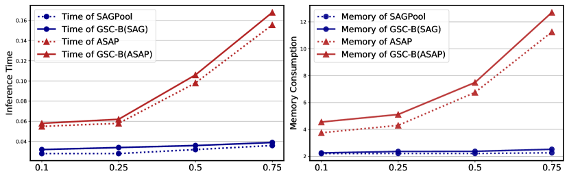
Figure 3: Time (left), Memory (right) curve w.r.t sampling ratio.

Table 3: Comparison for self-correction and post-enhancement. The number in parentheses refers to the relative improvement.

Method	PROTEINS	NCI1	NCI109
SAGPool	73.26 (-)	69.88 (-)	70.07 (-)
w/ PGPE	73.35 (+0.11)	70.32 (+0.44)	70.30 (+0.23)
w/ GSC	$74.36$ (+1.10)	$72.38$ (+2.50)	$72.03$ (+1.96)

6.2.1 Complexity Analysis

The graph self-correction needs to additionally add the steps of compensated information calculation and feedback. The time complexity of phase 1 depends on the based pooling module. It takes $O(Nd^{2})+O(|\mathcal{E}|d)$ to derive the compensated graph in phase 2, and $O(Nd)$ to perform the fusion in phase 3. We further analysis the trade-off between complexity and accuracy through the following three aspects.

First, we compare the inference time and the training memory consumption of the methods. As shown in Figure 3, GSC only increases marginal computational overhead over the baselines. Second, we compare the efficiency of GSC and the most competitive module of ASAP [33]. Using SAGPool [21] as a baseline, and a metric defined as the average accuracy improvement $\Delta_{\text{Acc}}$ divided by increased time cost $\Delta_{\text{Time}}$, GSC achieves a score of $3.75$ while ASAP only obtains $0.33$. We provide detailed results in Appendix. Third, we evaluate the contribution of the increased model capacity. We establish another baseline module named as Pooled Graph Post-Enhancement (PGPE), which leverages a single GCN layer to update the coarsened graph after each hierarchical pooling layer. In this case, the GNNs equipped with PGPE and GSC possess the same number of parameters, whose results are summarized in Table 3. Clearly, the post-enhancement strategy (‘w/ PGPE’) fails in improving the embedding quality and obtains slight performance gain, while the self-correction during pooling process (‘w/ GSC’) is much more effective and achieves over 1.5% accuracy improvement on average.

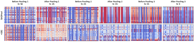
Figure 4: Visualization of node embeddings of a graph before and after pooling layers on PROTEINS. Visualization maps are stretched to be vertically aligned, and a node is represented by a row. The number of nodes for each embedding matrix is given above the figure. On the SAGPool baseline, the high homogeneity of node embeddings is observed (the same as findings in [30]), meaning the graph pooling process exacerbate the information loss. The GSC instead preserves more diversified representation patterns from the original features.

6.3 Evaluation of Ensemble Muitiscale Learning

Next we answer to the second question by performing evaluations on the ensemble framework depicted in Figure 2 and validating the effect of GSC and DBR.

6.3.1 How the GSC Helps the Ensemble Learning

Quantitative result. We particularly compare the ensemble performance between with and without graph self-correction mechanism on the pooling process. The results are separately given in Table 2 (methods denoted with ‘+’) and Table 1. Table 1 illustrates the failure of ensemble strategy on boosting multiscale GNNs built on baseline pooling modules. In contrast, for the multiscale GNNs equipped with GSC procedure (‘GSC-C’ or ‘GSC-B’), the ensemble strategy (‘GSC-C+’ or ‘GSC-B+’) successfully achieves over $0.5\%$ average accuracy improvement on the even stronger baselines. More experimental results under different model settings are given in Appendix.

Qualitative analysis. Intuitively, the failure of classic ensemble strategy on multiscale GNNs is natural if the node representations possess similar patterns, since the stacking-style ensemble learning requires diversified information. We conduct an exploring analysis to validate this intuition. Figure 4 shows the phenomenons that are in line with our expectations: nodes become severely homogenized after the second graph pooling process with SAGPool [21], while the GSC mechanism helps relieve this issue. The visualization analysis has provided a deeper insight into the beneficial effect of graph self-correction on the ensemble multiscale learning, that is, promoting the preserving of nodes discrepancy in the coarse graph via restoring the fine graph, which further helps to increase the diversity of input information of the ensemble model.

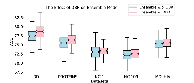
Figure 5: Comparison between ensemble models training with (pink) and without (lightblue) the diversity boosting regularizer. Hyper-parameter settings are deferred to Appendix. The box plot shows the mean accuracy and the standard deviation.

6.3.2 How the DBR Helps the Ensemble Learning

We conduct a comparison study on the ensemble multiscale GNNs equipped with GSC, under the difference between training with and without the proposed DBR. The results are displayed in Figure 5, which verify that DBR can jointly improve the ensemble performance with the GSC mechanism. One can see that DBR achieves smaller standard deviation under the 10-fold cross validation, which means the diversified graph embeddings indeed provide a more comprehensive characterization of the input graph, and thus improve the training stability. The effectiveness of DBR and GSC on enhancing the representation diversity provides a general and effective solution to build the ensemble-based multiscale graph classification networks.

Table 4: The effect of DBR for exceeding SOTAs on MOLHIV.

Method	Baseline	+ Ensemble	+ DBR
GCN	$76.16_{\pm 0.96}$	$77.54_{\pm 0.83}$	$\textbf{78.06}_{\pm 1.13}$
DeeperGCN	$77.50_{\pm 1.71}$	$78.63_{\pm 0.86}$	$\textbf{79.36}_{\pm 1.43}$

Performance on Deeper GNNs. We provide additional experiments to apply DBR for exceeding state-of-the-art (SOTA) GNNs on MOLHIV, which are usually deeper networks and adopt the global pooling layer for generating graph-level embeddings, since the dataset have graphs with fewer nodes. We select the GCN [18] and DeeperGCN [22] as evaluation baselines, and construct the ensemble-style model on them (details are deferred to Appendix. The results are shown in Table 4. It’s clear to observe performance improvements by applying the diversity boosting regularizer on these SOTA models, which again verifies its effectiveness and generalization ability.

7 Conclusion

Compared to various multiscale graph feature extraction frameworks, we provide an orthogonal perspective to establish a practical ensemble model. The proposed graph self-correction not only leads to significant improvements over existing graph pooling methods by serving as a plug-in component, but also contributes to promoting the ensemble diversity on node-level embeddings. Working together with the new diversity boosting regularizer that enhances diversity on graph-level embeddings, they jointly lead the ensemble model to achieve superior performances.

References

- [1] Filippo Maria Bianchi, Daniele Grattarola, and Cesare Alippi. Spectral clustering with graph neural networks for graph pooling. 2020.
- [2] Joan Bruna, Wojciech Zaremba, Arthur Szlam, and Yann LeCun. Spectral networks and locally connected networks on graphs. arXiv preprint arXiv:1312.6203, 2013.
- [3] Joao Carreira, Pulkit Agrawal, Katerina Fragkiadaki, and Jitendra Malik. Human pose estimation with iterative error feedback. In Proceedings of the IEEE conference on computer vision and pattern recognition, pages 4733–4742, 2016.
- [4] Haochen Chen, Bryan Perozzi, Yifan Hu, and Steven Skiena. Harp: Hierarchical representation learning for networks. arXiv preprint arXiv:1706.07845, 2017.
- [5] Balázs Csanád Csáji et al. Approximation with artificial neural networks. Faculty of Sciences, Etvs Lornd University, Hungary, 24(48):7, 2001.
- [6] Michaël Defferrard, Xavier Bresson, and Pierre Vandergheynst. Convolutional neural networks on graphs with fast localized spectral filtering. In Advances in neural information processing systems, pages 3844–3852, 2016.
- [7] Chenhui Deng, Zhiqiang Zhao, Yongyu Wang, Zhiru Zhang, and Zhuo Feng. Graphzoom: A multi-level spectral approach for accurate and scalable graph embedding. In International Conference on Learning Representations, 2019.
- [8] Thomas G Dietterich. Ensemble methods in machine learning. In International workshop on multiple classifier systems, pages 1–15. Springer, 2000.
- [9] Hongyang Gao and Shuiwang Ji. Graph u-nets. arXiv preprint arXiv:1905.05178, 2019.
- [10] Will Hamilton, Zhitao Ying, and Jure Leskovec. Inductive representation learning on large graphs. In Advances in neural information processing systems, pages 1024–1034, 2017.
- [11] Muhammad Haris, Gregory Shakhnarovich, and Norimichi Ukita. Deep back-projection networks for super-resolution. In Proceedings of the IEEE conference on computer vision and pattern recognition, pages 1664–1673, 2018.
- [12] Mikael Henaff, Joan Bruna, and Yann LeCun. Deep convolutional networks on graph-structured data. arXiv preprint arXiv:1506.05163, 2015.
- [13] Weihua Hu, Matthias Fey, Marinka Zitnik, Yuxiao Dong, Hongyu Ren, Bowen Liu, Michele Catasta, and Jure Leskovec. Open graph benchmark: Datasets for machine learning on graphs. arXiv preprint arXiv:2005.00687, 2020.
- [14] Jingjia Huang, Zhangheng Li, Nannan Li, Shan Liu, and Ge Li. Attpool: Towards hierarchical feature representation in graph convolutional networks via attention mechanism. In Proceedings of the IEEE International Conference on Computer Vision, pages 6480–6489, 2019.
- [15] Michal Irani and Shmuel Peleg. Improving resolution by image registration. CVGIP: Graphical models and image processing, 53(3):231–239, 1991.
- [16] Md M Islam, Xin Yao, and Kazuyuki Murase. A constructive algorithm for training cooperative neural network ensembles. IEEE Transactions on neural networks, 14(4):820–834, 2003.
- [17] Amir Hosein Khasahmadi, Kaveh Hassani, Parsa Moradi, Leo Lee, and Quaid Morris. Memory-based graph networks. arXiv preprint arXiv:2002.09518, 2020.
- [18] Thomas N Kipf and Max Welling. Semi-supervised classification with graph convolutional networks. arXiv preprint arXiv:1609.02907, 2016.
- [19] Anders Krogh and Jesper Vedelsby. Neural network ensembles, cross validation, and active learning. Advances in neural information processing systems, 7:231–238, 1994.
- [20] Alex Kulesza and Ben Taskar. Determinantal point processes for machine learning. arXiv preprint arXiv:1207.6083, 2012.
- [21] Junhyun Lee, Inyeop Lee, and Jaewoo Kang. Self-attention graph pooling. arXiv preprint arXiv:1904.08082, 2019.
- [22] Guohao Li, Chenxin Xiong, Ali Thabet, and Bernard Ghanem. Deepergcn: All you need to train deeper gcns. arXiv preprint arXiv:2006.07739, 2020.
- [23] Jia Li, Yu Rong, Hong Cheng, Helen Meng, Wenbing Huang, and Junzhou Huang. Semi-supervised graph classification: A hierarchical graph perspective. In The World Wide Web Conference, WWW ’19, page 972–982, New York, NY, USA, 2019. Association for Computing Machinery.
- [24] Ke Li, Bharath Hariharan, and Jitendra Malik. Iterative instance segmentation. In Proceedings of the IEEE conference on computer vision and pattern recognition, pages 3659–3667, 2016.
- [25] Maosen Li, Siheng Chen, Ya Zhang, and Ivor W Tsang. Graph cross networks with vertex infomax pooling. arXiv preprint arXiv:2010.01804, 2020.
- [26] Yujia Li, Daniel Tarlow, Marc Brockschmidt, and Richard Zemel. Gated graph sequence neural networks. arXiv preprint arXiv:1511.05493, 2015.
- [27] Jiongqian Liang, Saket Gurukar, and Srinivasan Parthasarathy. Mile: A multi-level framework for scalable graph embedding. arXiv preprint arXiv:1802.09612, 2018.
- [28] William Lotter, Gabriel Kreiman, and David Cox. Deep predictive coding networks for video prediction and unsupervised learning. arXiv preprint arXiv:1605.08104, 2016.
- [29] Yao Ma, Suhang Wang, Charu C Aggarwal, and Jiliang Tang. Graph convolutional networks with eigenpooling. In Proceedings of the 25th ACM SIGKDD International Conference on Knowledge Discovery & Data Mining, pages 723–731, 2019.
- [30] Diego Mesquita, Amauri H Souza, and Samuel Kaski. Rethinking pooling in graph neural networks. arXiv preprint arXiv:2010.11418, 2020.
- [31] Christopher Morris, Nils M Kriege, Franka Bause, Kristian Kersting, Petra Mutzel, and Marion Neumann. Tudataset: A collection of benchmark datasets for learning with graphs. arXiv preprint arXiv:2007.08663, 2020.
- [32] Tianyu Pang, Kun Xu, Chao Du, Ning Chen, and Jun Zhu. Improving adversarial robustness via promoting ensemble diversity. arXiv preprint arXiv:1901.08846, 2019.
- [33] Ekagra Ranjan, Soumya Sanyal, and Partha P Talukdar. Asap: Adaptive structure aware pooling for learning hierarchical graph representations. In AAAI, pages 5470–5477, 2020.
- [34] Ye Ren, Le Zhang, and Ponnuthurai N Suganthan. Ensemble classification and regression-recent developments, applications and future directions. IEEE Computational intelligence magazine, 11(1):41–53, 2016.
- [35] Abhinav Shrivastava and Abhinav Gupta. Contextual priming and feedback for faster r-cnn. In European conference on computer vision, pages 330–348. Springer, 2016.
- [36] Zhuowen Tu and Xiang Bai. Auto-context and its application to high-level vision tasks and 3d brain image segmentation. IEEE transactions on pattern analysis and machine intelligence, 32(10):1744–1757, 2009.
- [37] Petar Veličković, Guillem Cucurull, Arantxa Casanova, Adriana Romero, Pietro Liò, and Yoshua Bengio. Graph attention networks. In International Conference on Learning Representations, 2018.
- [38] Oriol Vinyals, Samy Bengio, and Manjunath Kudlur. Order matters: Sequence to sequence for sets. arXiv preprint arXiv:1511.06391, 2015.
- [39] Yu Guang Wang, Ming Li, Zheng Ma, Guido Montufar, Xiaosheng Zhuang, and Yanan Fan. Haar graph pooling. In International Conference on Machine Learning, pages 9952–9962. PMLR, 2020.
- [40] Zhenqin Wu, Bharath Ramsundar, Evan N Feinberg, Joseph Gomes, Caleb Geniesse, Aneesh S Pappu, Karl Leswing, and Vijay Pande. Moleculenet: a benchmark for molecular machine learning. Chemical science, 9(2):513–530, 2018.
- [41] Keyulu Xu, Weihua Hu, Jure Leskovec, and Stefanie Jegelka. How powerful are graph neural networks? In International Conference on Learning Representations, 2018.
- [42] Zhitao Ying, Jiaxuan You, Christopher Morris, Xiang Ren, Will Hamilton, and Jure Leskovec. Hierarchical graph representation learning with differentiable pooling. In Advances in neural information processing systems, pages 4800–4810, 2018.
- [43] Fuzhen Zhang. Matrix theory: basic results and techniques. Springer Science & Business Media, 2011.
- [44] Le Zhang, Zenglin Shi, Ming-Ming Cheng, Yun Liu, Jia-Wang Bian, Joey Tianyi Zhou, Guoyan Zheng, and Zeng Zeng. Nonlinear regression via deep negative correlation learning. IEEE Transactions on Pattern Analysis and Machine Intelligence, 2019.
- [45] Muhan Zhang, Zhicheng Cui, Marion Neumann, and Yixin Chen. An end-to-end deep learning architecture for graph classification. In Thirty-Second AAAI Conference on Artificial Intelligence, 2018.