Detecting Anomalous Swarming Agents with Graph Signal Processing
Abstract
Collective motion among biological organisms such as insects, fish, and birds has motivated considerable interest not only in biology but also in distributed robotic systems. In a robotic or biological swarm, anomalous agents (whether malfunctioning or nefarious) behave differently than the normal agents and attempt to hide in the “chaos” of the swarm. By defining a graph structure between agents in a swarm, we can treat the agents’ properties as a graph signal and use tools from the field of graph signal processing to understand local and global swarm properties. Here, we leverage this idea to show that anomalous agents can be effectively detected using their impacts on the graph Fourier structure of the swarm.
Index Terms— swarming, graph signal processing, anomaly detection
1 Introduction
Collective motion in biological systems such as insect swarms, fish schools, and bird flocks are visually striking emergent behaviors that have motivated considerable research in biology, physics, and engineering [1, 2, 3, 4, 5]. Due to the distributed nature of swarming systems, graph theory has found considerable utility in the analysis and synthesis of swarming systems by modeling the communications or other interactions between swarming agents as a graph structure [6, 7]. Recently, tools from computational topology have been applied to understanding the structure of swarms in terms of connected sub-components as well as the presence of holes and voids [8, 9]. These tools explicitly rely on the parametric construction of a graph structure between agents.
This topological approach was further extended in [10] to analyze how the local and global “order” of swarm properties varies with respect to the graph structure. The analysis in [10] employed the field of graph signal processing (GSP) and graph Fourier analysis to show that common swarm states were highly structured (i.e., band-limited) when viewed in the graph Fourier domain. Broadly speaking, GSP builds on its roots in spectral graph theory [11] and algebraic signal processing [12] to generalize concepts from classical signal processing to signals defined on the vertices of irregular domains modeled by graphs [13, 14, 15, 16].
Anomaly detection [17] is among the application areas considered in the seminal GSP works [15, 18]. Since the initial work that considered temperature sensor networks [15] and more generally abstract sensor networks [18], GSP-based anomaly detection has been applied to a number of areas, including power systems [19, 20], social networks [16], and image processing [21]. At a high level, these techniques exploit (generally low-pass) structure in the graphical Fourier transform (GFT) of some signal defined on the vertices of a graph, and then threshold on the signal content after (graph) filtering to remove this structure [16]. We note that this class of problem is fundamentally different from detecting an anomalous graph structure in a network, itself a well studied problem [22].
In this work, we show how the GFT structure of swarms revealed in [10] can be used to design “graph filters” that operate on the swarm state to detect agents within the swarm whose dynamics (and thus behavior) are fundamentally different from the bulk of the swarm. These anomalous agents have behaviors that differ in subtle ways from the rest of the swarm; from a purely kinematic perspective the anomalous trajectories are consistent with the non-anomalous agents. Instead, these behaviors are detected through interaction and comparison with their neighbors that manifest in the GFT domain as outliers. To our knowledge, this work is the initial adaptation of GSP techniques to the swarming domain, and the detection problems herein are challenging enough that multiple swarm measurements are needed for effective detection, demonstrating an anomaly detection problem where the signal is not only time-varying as in [23], but with a time varying graph, as well. This work is related to, but distinct from, the inference of dynamical parameters [24] and the identification of collective states [25, 8, 9], as this work more closely resembles clustering (i.e., unsupervised learning) of distinct behavior regimes within the swarm. More generally, this work falls under fault detection in swarms [26], and addresses similar problems as [27], which uses neural networks to identify joint collective anomalies, comprising a more data intensive approach.
In the following, we first review some GSP and swarming preliminaries. Next, we briefly discuss how to interpret swarming in a GSP context and define two GSP approaches to the detection of anomalous agents in a swarm. We then consider both approaches in a range of scenarios using swarming simulations of [1] and [4], discussing how to leverage their unique graph Fourier signatures, and analyze the resulting anomaly detectors using detection theory. We conclude with summary remarks and discuss future directions.
2 GSP Background
A graph consists of a collection of vertices and edges connecting nodes and . The graph adjacency matrix mathematically represents interactions in a graph, with nonzero entries indicating the presence of an edge . In this work, we are concerned with non-negative weighted undirected graphs, so . The degree matrix is a diagonal matrix whose entries account for the total number of connections for each node and is defined as . The (combinatorial) graph Laplacian is defined as . A related matrix, the normalized Laplacian, is defined for connected graphs by and extends to general graphs several nice properties of the Laplacian that only hold for certain regular graphs [11].
GSP is concerned with the analysis of signals or functions defined on the vertices of a graph. Let be a so-called graph signal defined on that takes values in some finite dimensional Hilbert space. We adopt the shorthand convention that for the th vertex of . Over the last decade, most GSP efforts have focused on extending techniques defined in classical signal processing to signals defined over graphs, such as filtering and multiple signal transformations including the GFT. In a natural definition for non-negative weighted symmetric graphs, the GFT uses the eigenvectors of as basis functions instead of the complex exponentials used in the Fourier transform. However, [10] demonstrated that may be better suited for analysis of swarms. Using the eigendecomposition , with a unitary matrix of eigenvectors, and a diagonal matrix of eigenvalues in increasing order, the GFT of a graph signal is defined as and the corresponding inverse GFT as . Using this definition of the GFT, the eigenvalues are a natural generalization of frequency that are no longer evenly spaced in general, but will be in the interval . This further suggests an intuitive mechanism to define graph filters using the eigendecomposition. Let be a diagonal matrix, then is a filtered graph signal where the filter has “frequency response” at frequency .
3 Swarm Models
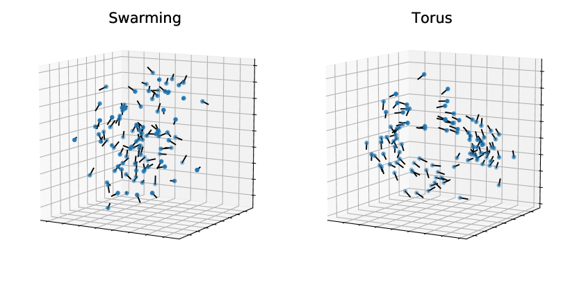
In this work, we will consider anomalous agents in an otherwise homogeneous swarm using two different swarming models: the biologically inspired model of [1] and the swarmalator model of [4]. The model in [1] uses disjoint behavior regions for repulsion, alignment, and attraction. Depending on the relative radii of these regions, the angle of a blind-spot behind each agent, and the amount of noise, the swarm dynamics will produce one of four steady states. In the absence of an alignment region, the dynamics produce a disorganized “swarming” state characterized by low local and global alignment in velocity and minimal collective displacement. When the region of alignment is larger than the region of repulsion, but still small relative to the region of attraction, the swarm tends to form three-dimensional torus-like structures, with a high level of local alignment in velocity but overall low global alignment and little collective displacement. As the alignment region approaches the attraction region, two additional collective states form, both with higher global velocity alignment and collective displacement than the swarming and torus states. Here, we focus on the first two states due to their apparent disorganization, presumably making an anomalous agent harder to detect (see Fig. 1).
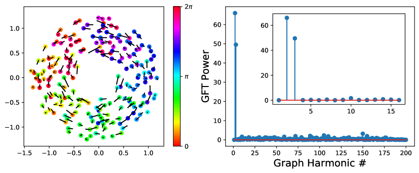
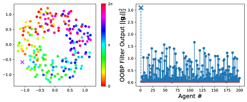
The swarmalator model was developed to understand joint swarming and synchronization behaviors, combining spatial attraction and repulsion with an auxiliary phase . This phase can modulate the sign of the spatial attraction/repulsion and is itself governed by dynamics in the vein of the Kuramoto model [28]. Of the several steady states observed in [4] we focus on the active wave state in two dimensions, where the agents form counter-rotating (roughly) phase-ordered rings that exhibit considerable dynamism in both the position and phase states (see Fig. 2, left panel).
4 Methods
The necessary ingredients for performing GSP analysis are the specification of a graph and a function defined on the vertices of that graph. For a collection of swarming entities with positions and velocities both (time indices surpressed), following [10] we define each agent as a vertex in a graph, and for each instance in time we construct an adjacency matrix (, otherwise ), where . Depending on the scenario, we consider different graph signals. For the model of [1] we consider the normalized velocity and the adjusted position where . For the analysis of swarmalators we use the signal .
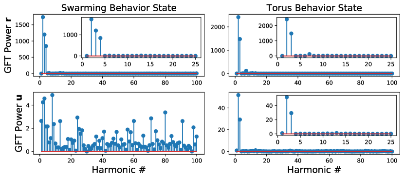
With these graph and graph signal definitions, using the GFT derived from we have from [10] that both the model of [1] and swarmalators exhibit spectral concentration in a few graph Fourier harmonics (see Fig. 3 and Fig. 2, right panel). Furthermore, these harmonics are low frequency, indicating local alignment of the graph signal with respect to the graph topology.
This spectral concentration immediately suggests two approaches for anomaly detection: 1) a graph filter approach with filters defined by where if and otherwise and is a set of graph frequencies expected not to be common in nominal swarms, and 2) using the intuition that an anomalous agent should be different in “smoothness” than the rest of the swarm, the high-pass filter , which has been suggested as a measure of local graph smoothness for a graph signal [16]. We call the first approach out-of-band power (OOBP) and the second local graph smoothness (LGS). In either case, the input graph signal is filtered to generate , and is used as a threshold statistic for the detection of an anomalous agent in the swarm (c.f., [18, 19, 20]).
5 Results
We ran the swarming model of [1] with 100 agents (99 normal, 1 anomalous) and the swarmalator model with 200 agents (199 normal, and 1 anomalous). We ran each with a few different sets of parameters for both the nominal and anomalous agents. For the model of [1], we ran 4 cases:
-
•
Case 1: Nominal behavior is Swarming, anomalous agent has slightly larger repulsion region ( is the graph signal)
-
•
Case 2: Nominal behavior is Torus, anomalous agent has slightly larger repulsion region (same anomaly as Case 1, is the graph signal)
-
•
Case 3: Nominal behavior is Torus, anomalous agent has no alignment region ( is the graph signal)
-
•
Case 4: Nominal behavior is Swarming, anomalous agent has large alignment region ( is the graph signal)
For the swarmalator model, the nominal behavior of positional attraction to like phases and phase repulsion to nearby phases is defined by parameters , and the anomaly was parameterized at for positional repulsion to like phases and various values of in that varies the strength of the phase repulsion and attraction, using the model definitions as in [4, Fig. 4]. We use as the graph signal, and we denote this Case 5.
We define OOBP filters for each case based on the nominal and anomalous behaviors. For both Case 1 and 2, the nominal is lowpass (Fig. 3, top row) so we use the highpass filters and , respectively. For Case 3, is lowpass (Fig. 3, bottom right) and we use the same filter as Case 2. Despite the bandlimited nature of these signals, we found that the exclusion of the first harmonic improved detection. For Case 4, we expect the nominal swarm state to be spectrally flat (Fig. 3, bottom left) and an anomaly with a large alignment range to contribute to low frequency components, so our OOBP filter should be lowpass. We find that performed well. For Case 5, the signal is bandlimited (Fig. 2, right), and the bandstop filter produced excellent results.
While the LGS approach is already defined by a given swarm’s graph, note that since anomalies in Case 4 are expected to appear in low frequencies, they will have low values in the LGS approach, but high values for the remaining cases. We set the direction of our detector accordingly.
Each of these model parameterizations was run with 100 Monte Carlo runs that varied the initial state of each agent and then iterated for 1500 time steps to allow for the swarm to stabilize. After that, the graph was defined from agent states as described above and the two approaches OOBP and LGS were evaluated at discrete time steps 50 time steps apart to create swarm “snapshots” to allow for correlations in swarm state to die out. The results of the norm squared of the filtered signal at each agent were summed over the snapshots to produce the measurements that were thresholded to define our anomaly detector. The area under the receiver operating characteristic (ROC) curve, empirically estimating the probability that an anomalous agent whose parameters are uniformly randomly selected from those explored would have a higher statistic value than a randomly chosen nominal agent, providing an indication of how effectively the threshold statistic can be used to detect anomalous agents [29], is shown in Fig. 4.
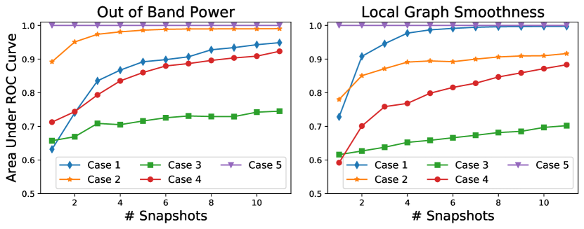
These curves show that there is a range of efficacy of both detectors across the cases considered, although we note that all of them produce areas substantially greater than 0.5 (random chance), and all appear to improve as the number of snapshots (analogous to integration time) increases. It is clear that Case 5 appears to be an extremely easy detection problem, whereas Case 3 is the most challenging. Viewing a typical example from Case 5 (Fig. 5) we see that the anomalous agent is somewhat out of phase from the rest of the swarm, but may be challenging to visually identify if not explicitly marked. However, the filtered response is a clear outlier, consistent with the intuition behind our approach. The more challenging cases have considerable overlap in the distributions of the filtered signals. We note that detecting the repulsion-based anomaly in Cases 1 and 2 appears to be considerably easier than detecting anomalous alignment behaviors in Cases 3 and 4. Anecdotally we do see that more repulsive agents will occasionally appear farther from than nominal agents, whereas the alignment effects are generally unnoticeable visually. Another interesting facet of these results is that OOBP appears to be a more effective detection mechanism, except in Case 1. Why this is the case despite such a concentrated GFT response of the nominal behavior we leave to future research.
6 Conclusion
In summary, we demonstrated how the GFT structure of swarms could be leveraged to detect anomalous agent behaviors in a number of scenarios. We considered two different filter-based approaches and used a variety of graph signals as the subjects of the analysis. Overall, we demonstrated that the relative efficacy of these approaches appears highly dependent on the specific context. Using detection-theoretic ROC analysis we demonstrated that accumulating information over several snapshots of the swarming data may be needed to have effective detectors in the most challenging cases.
This work indicates a number of potential future directions in not only anomaly detection in swarms but more generally in the application of GSP techniques. Further analysis of the cases considered here is warranted, and additional swarming models and anomalies could be analyzed as well. GSP techniques that analyze both the vertex and time domains simultaneously could be incorporated [21], although this would require handling time-varying graphs (rather than the independent manner in which they were treated here). In principle, this work could be combined with distributed graph filtering techniques to perform self-anomaly detection within the swarm. Finally, we note that the the techniques here could be adapted to behavior discrimination and classification of agents in a swarm such as leader vs. follower behaviors.
References
- [1] Iain D Couzin, Jens Krause, Richard James, Graeme D Ruxton, and Nigel R Franks, “Collective memory and spatial sorting in animal groups,” Journal of theoretical biology, vol. 218, no. 1, pp. 1–12, 2002.
- [2] David JT Sumpter, Collective animal behavior, Princeton University Press, 2010.
- [3] Tamás Vicsek and Anna Zafeiris, “Collective motion,” Physics reports, vol. 517, no. 3-4, pp. 71–140, 2012.
- [4] Kevin P O’Keeffe, Hyunsuk Hong, and Steven H Strogatz, “Oscillators that sync and swarm,” Nature communications, vol. 8, no. 1, pp. 1–13, 2017.
- [5] Kevin M Passino, Biomimicry for optimization, control, and automation, Springer Science & Business Media, 2005.
- [6] Ali Jadbabaie, Jie Lin, and A Stephen Morse, “Coordination of groups of mobile autonomous agents using nearest neighbor rules,” IEEE Transactions on automatic control, vol. 48, no. 6, pp. 988–1001, 2003.
- [7] Reza Olfati-Saber, “Flocking for multi-agent dynamic systems: Algorithms and theory,” IEEE Transactions on automatic control, vol. 51, no. 3, pp. 401–420, 2006.
- [8] Chad M Topaz, Lori Ziegelmeier, and Tom Halverson, “Topological data analysis of biological aggregation models,” PloS one, vol. 10, no. 5, pp. e0126383, 2015.
- [9] Padraig Corcoran and Christopher B Jones, “Modelling topological features of swarm behaviour in space and time with persistence landscapes,” IEEE Access, vol. 5, pp. 18534–18544, 2017.
- [10] Kevin Schultz, Marisel Villafañe Delgado, Elizabeth P Reilly, Anshu Saksena, and Grace M Hwang, “Analyzing collective motion using graph fourier analysis,” arXiv preprint: arXiv:2103.08583, 2021.
- [11] Fan RK Chung and Fan Chung Graham, Spectral graph theory, Number 92. American Mathematical Soc., 1997.
- [12] Markus Puschel and José MF Moura, “Algebraic signal processing theory: Foundation and 1-d time,” IEEE Transactions on Signal Processing, vol. 56, no. 8, pp. 3572–3585, 2008.
- [13] David Shuman, Sunil Narang, Pascal Frossard, Antonio Ortega, and Pierre Vandergheynst, “The emerging field of signal processing on graphs: Extending high-dimensional data analysis to networks and other irregular domains,” IEEE Signal Processing Magazine, vol. 3, no. 30, pp. 83–98, 2013.
- [14] Aliaksei Sandryhaila and José MF Moura, “Discrete signal processing on graphs,” IEEE Transactions on Signal Processing, vol. 61, no. 7, pp. 1644–1656, 2013.
- [15] Aliaksei Sandryhaila and Jose MF Moura, “Discrete signal processing on graphs: Frequency analysis,” IEEE Transactions on Signal Processing, vol. 62, no. 12, pp. 3042–3054, 2014.
- [16] Raksha Ramakrishna, Hoi To Wai, and Anna Scaglione, “A user guide to low-pass graph signal processing and its applications: Tools and applications,” IEEE Signal Processing Magazine, vol. 37, no. 6, pp. 74–85, 2020.
- [17] Varun Chandola, Arindam Banerjee, and Vipin Kumar, “Anomaly detection: A survey,” ACM computing surveys (CSUR), vol. 41, no. 3, pp. 1–58, 2009.
- [18] Hilmi E Egilmez and Antonio Ortega, “Spectral anomaly detection using graph-based filtering for wireless sensor networks,” in 2014 IEEE International Conference on Acoustics, Speech and Signal Processing (ICASSP). IEEE, 2014, pp. 1085–1089.
- [19] Elisabeth Drayer and Tirza Routtenberg, “Detection of false data injection attacks in smart grids based on graph signal processing,” IEEE Systems Journal, 2019.
- [20] Raksha Ramakrishna and Anna Scaglione, “Detection of false data injection attack using graph signal processing for the power grid,” in 2019 IEEE Global Conference on Signal and Information Processing, 2019.
- [21] Francesco Verdoja and Marco Grangetto, “Graph laplacian for image anomaly detection,” Machine Vision and Applications, vol. 31, no. 1, pp. 1–16, 2020.
- [22] Leman Akoglu, Hanghang Tong, and Danai Koutra, “Graph based anomaly detection and description: a survey,” Data mining and knowledge discovery, vol. 29, no. 3, pp. 626–688, 2015.
- [23] Gabriela Lewenfus, Wallace Alves Martins, Symeon Chatzinotas, and Björn Ottersten, “On the use of vertex-frequency analysis for anomaly detection in graph signals,” Anais do XXXVII Simpósio Brasileiro de Telecomunicações e Processamento de Sinais, 2019.
- [24] Yael Katz, Kolbjørn Tunstrøm, Christos C Ioannou, Cristián Huepe, and Iain D Couzin, “Inferring the structure and dynamics of interactions in schooling fish,” Proceedings of the National Academy of Sciences, vol. 108, no. 46, pp. 18720–18725, 2011.
- [25] Matthew Berger, Lee M Seversky, and Daniel S Brown, “Classifying swarm behavior via compressive subspace learning,” in 2016 IEEE International Conference on Robotics and Automation (ICRA). IEEE, 2016.
- [26] Liguo Qin, Xiao He, and DH Zhou, “A survey of fault diagnosis for swarm systems,” Systems Science & Control Engineering: An Open Access Journal, vol. 2, no. 1, pp. 13–23, 2014.
- [27] Hyojung Ahn, Han-Lim Choi, Minguk Kang, and SungTae Moon, “Learning-based anomaly detection and monitoring for swarm drone flights,” Applied Sciences, vol. 9, no. 24, pp. 5477, 2019.
- [28] Yoshiki Kuramoto, “International symposium on mathematical problems in theoretical physics,” Lecture notes in Physics, vol. 30, pp. 420, 1975.
- [29] James A Hanley and Barbara J McNeil, “The meaning and use of the area under a receiver operating characteristic (roc) curve.,” Radiology, vol. 143, no. 1, pp. 29–36, 1982.