Asymptotic and Finite-time Cluster Synchronization of Neural Networks via Two Different Controllers

Abstract

In this paper, by using pinning impulse controller and hybrid controller respectively, the research difficulties of asymptotic synchronization and finite time cluster synchronization of time-varying delayed neural networks are studied. On the ground of Lyapunov stability theorem and Lyapunov-Razumikhin method, a novel sufficient criterion on asymptotic cluster synchronization of time-varying delayed neural networks is obtained. Utilizing Finite time stability theorem and hybrid control technology, a sufficient criterion on finite-time cluster synchronization is also obtained. In order to deal with time-varying delay and save control cost, pinning pulse control is introduced to promote the realization of asymptotic cluster synchronization. Following the idea of pinning control scheme, we design a progressive hybrid control to promote the realization of finite time cluster synchronization. Finally, an example is given to illustrate the theoretical results.

1 Introduction

Synchronization in complex networks refers to a evolutionary process where two or more chaotic systems improve their behavior to achieve a common phenomenon under certain coupling conditions or under certain forces. It’s an important topic that have been captured by many experts and scholars from various fields of research [1, 2, 3, 4, 5, 6], such as physical science, natural science, mathematics, communication, and engineering. Because of that, different types of synchronization protocols have been studied in detail. For example, projective synchronization [7, 8, 9], cluster synchronization [10, 11, 12, 13, 14, 15], complete synchronization [16], generalized synchronization [17], phase synchronization [18], lag synchronization [19], and so on.

Sometimes it takes a lot of people to achieve a goal, and different aims may be implemented by different people in real life, such as the division of research teams and the setting of government function departments. Because of different tasks, they have to achieve different goals. The same is true in neural networks. Each node in the same part wants to achieve the same goal, nodes in the different clusters want to achieve different goals, this is the so-called cluster synchronization. Cluster synchronization has important applications in science [20] and Bioengineering [21]. During the past few years, cluster synchronization has been widely studied by a large number of researchers, see [10, 11, 12, 13, 14, 15, 22, 23, 24, 25] and the relevant references. In an attempt to investigate cluster synchronization of complex systems, there have been many results related to cluster synchronization of coupled systems. This is not only because cluster synchronization has unusual correlations between network subsystems, but also because many coupled networks can exhibit excellent clustering characteristic. Additionally, As we all know, time delay is an ubiquitous phenomenon in physical complex networks. This is inevitable and may lead to a undesirable state of the system [26]. Therefore, the influence of time delay should be considered. As a result, it is essential to investigate cluster synchronization of coupled neural networks with time-varying delay.

Because of the complexity of the network structure, researchers have proposed many effective methods to synchronize the complex networks, some effective methods are pinning control [27, 28, 29], impulsive control [30, 31, 32], intermittent control [33], adaptive control [34], feedback control [25, 35, 36], and so on. Impulse effect is a common phenomenon due to the instantaneous disturbance at some time. These phenomena are described by impulsive differential equation which have been used efficiently in modeling many practical problems that arise in the fields of engineering, physics, and science. Regarding to this, pinning impulsive control becomes a practically external control approach which is famous for low cost and energy-saving. Pinning impulsive control is characterized by adding impulsive controllers on only a fraction of network nodes. [31] investigated the pinning synchronization problem of stochastic impulsive networks using Lyapunov stability theory and pinning method. However, it only examined asymptotical synchronization and exponential synchronization of such dynamical networks in mean square. By introducing stochastic impulsive analysis technique and the selected nodes of the stochastic network are pinned at the impulse moment, authors in [22] discussed cluster synchronization of delayed stochastic neural networks under pinning impulsive control. A disadvantage of the above two papers is that they only considers the asymptotic behavior of the system as time approaches infinity.

In control theory, a considerable number of papers are focused on the utilization of pinning control to help complex networks achieve cluster synchronization. Based on the Lyapunov stability theory, the article [37] is devoted to study the cluster synchronization for network of a complex dynamical network of non-identical nodes with delayed and non-delayed coupling under a pinning control scheme. The finite-time and fixed-time cluster synchronization problem for complex networks with or without pinning control are studied in [38]. However, the systems in this paper are special coupled networks where use a concrete function $\rm sig^{p}(x)$. The major objective of [23] is to deal with cluster synchronization of coupled fractional-order neural networks with time delay, while the two control laws in this work is not pinning control but the control of all nodes in these networks. Based on it, we want to extend the idea of pinning control to control some of the key nodes in each cluster, and exert no control over the remaining nodes in the cluster, or only exert weak control over the remaining nodes, which is so-called hybrid control.

Based on above analysis, we study cluster synchronization of coupled neural networks with time-varying delay both on asymptotic cluster synchronization and on finite-time cluster synchronization. Unlike the literature [23] which is devoted to constant delay, we deal with time-varying delay, so the method in the literature [23] can’t be used here. We utilize Lyapunov-Razumikhin method to deal with time-vary delay. Two novel sufficient conditions are obtained on asymptotic and finite-time cluster synchronization of the neural networks by exerting pinning impulsive control and hybrid control, respectively. The article is arranged as follows. In section 2, some preliminaries on asymptotic and finite-time cluster synchronization are provided. In section 3, we give some major results. In section 4, a numerical example is given to check the effectiveness of the consequences. The final section is the conclusion of this paper.

2 Preliminaries

2.1 Model Description

Consider the following system which consists of $N$ coupled neural networks with time-varying delay, the $i$th neural network is described by

$$\left\{\begin{array}[]{c}\dot{x}_{i}(t)=-C_{i}x_{i}(t)+A_{i}f\left(x_{i}(t)\right)+B_{i}f\left(x_{i}(t-\tau(t))\right)+\sum\limits_{j=1}^{N}g_{ij}x_{j}(t)\\ +I_{i}+u_{i}(t),\\ x_{i}(t)=\phi_{i}(t),t\in\left[-\tau,0\right],\end{array}\right.$$ (1)

where $x_{i}(t)=\left(x_{i1}(t),x_{i2}(t),\cdots,x_{in}(t)\right)^{T}$ is the state vector of the $i$th neural network at time $t$, $C_{i}>0$(means a symmetrical positive determined matrix) denotes the self-inhibition rate, $A_{i}=\left(a_{lr}^{i}\right)_{n\times n}\in R^{n\times n}$ and $B_{i}=\left(b_{lr}^{i}\right)_{n\times n}\in R^{n\times n}$ are connection weight matrices and delayed connection weight matrices, respectively. $f(x)$ is the activation function at time $t$ , $\tau(t)$ is transmittal delay. We suppose there exists two constants $\tau$ and $\sigma$, render $0<\tau(t)<\tau$ and $\dot{\tau}(t)\leq\sigma<1$. $I_{i}\in R^{n}$ means a input from the outside of the system, $u_{i}(t)$ is the controller that will be designed below. The element $g_{ij}$ of a linear coupling matrix is expressed as that if there is a connection from node $i$ to another node $j$ , then $g_{ij}\neq 0$, otherwise $g_{ij}=0$. The diagonal terms of the matrix satisfy the following diffusion coupling conditions: $g_{ii}=-\sum\limits_{j=1,j\neq i}^{N}g_{ji}$.

2.2 Cluster Synchronization

Let$\{\mathscr{C}_{1},\cdots,\mathscr{C}_{M}\}$ be a partition of the set $\{1,\cdots,N\}$ , by which $\{1,\cdots,\\ N\}$ is divided into $M$ nonempty subsets, i.e. $\mathscr{C}_{l}\neq\phi$ and $\bigcup\limits_{l=1}^{M}{\mathscr{C}_{l}}=\{1,\cdots,N\}$. For each $l\in\{1,\cdots,N\}$, let $\widetilde{l}$ denotes the subscript of the subset where the number $l$ is, i.e. $l\in\mathscr{C}_{\widetilde{l}}$.

A network with $N$ nodes is said to reach asymptotic cluster synchronization if the state variables of the network satisfies $\lim\limits_{t\rightarrow\infty}\left\|x_{i}(t)-x_{j}(t)\right\|=0$ for ${\widetilde{i}=\widetilde{j}}$ and $\lim\limits_{t\rightarrow\infty}\left\|x_{i}(t)-x_{j}(t)\right\|\neq 0$ for ${\widetilde{i}\neq\widetilde{j}}$. Furthermore, A network with $N$ nodes is said to reach finite-time cluster synchronization if there exists a $t^{*}>t_{0}$ such that for ${\widetilde{i}=\widetilde{j}}$ ,$\lim\limits_{t\rightarrow t^{*}}\left\|x_{i}(t)-x_{j}(t)\right\|=0$ and $\|x_{i}(t)-x_{j}(t)\|=0$ for $t\geq t^{*}$.

Definition 1[23]. The function $H=(h_{ij}\in R^{m\times m})$ is said to belong to class $\mathscr{A}_{1}$, if it satisfies $h_{ij}\geq 0,h_{ii}=-\sum\limits_{j=1,j\neq i}^{m}h_{ij}$.

Definition 2 [23]. The function $H=(h_{ij}\in R^{m\times m})$ belongs to class $\mathscr{A}_{2}$, if it satisfies $\sum\limits_{j=1}^{m}h_{ij}=0$.

Assumption 1 [23]. For $i\in\mathscr{C}_{p},p=\{1,2,\cdots,M\}$, there exists $\xi_{p}>0$, for all $x,y\in R^{n}$, $\|f(x)-f(y)\|\leq\xi_{p}\|x-y\|$.

Assumption 2 [23]. If all $N$ nodes are divided into $M$ clusters, The Laplace matrix can be defined in the following form

$$\begin{array}[]{l}\left(\begin{array}[]{ccccc}\bar{A}_{11}&\bar{A}_{12}&\bar{A}_{13}&\cdots&\bar{A}_{1M}\\ \bar{A}_{21}&\bar{A}_{22}&\bar{A}_{23}&\cdots&\bar{A}_{2M}\\ \bar{A}_{31}&\bar{A}_{32}&\bar{A}_{33}&\cdots&\bar{A}_{3M}\\ \vdots&\vdots&\vdots&\ddots&\vdots\\ \bar{A}_{M1}&\bar{A}_{M2}&\bar{A}_{M3}&\cdots&\bar{A}_{MM}\end{array}\right),\end{array}$$

where $\bar{A}_{ij}\in R^{\left(v_{i}-v_{i-1}\right)\times\left(v_{j}-v_{j-1}\right)},\bar{A}_{pp}\in\mathscr{A}_{1},q=1,2,\cdots,M$, $\bar{A}_{pq}\in\mathscr{A}_{2},p,q=1,2,\cdots,M,p\neq q$.

2.3 Mathematical Preparation

Provided that the $N$ nodes can be divided into $M$ clusters, that is to say $\{1,2,\cdots,N\}=\mathscr{C}_{1}\cup\mathscr{C}_{2}\cup\cdots\cup\mathscr{C}_{M}$, where $\mathscr{C}_{p}=\left\{v_{p-1}+1,v_{p-1}+2,\cdots,v_{p}\right\}$, $p=1,2,\cdots,M$ and $v_{0}=0$, $v_{M}=N$, $v_{p-1}<v_{p}$. It is necessary to assume that the coefficients of system (1) meet $C_{v_{p-1}+1}=C_{v_{p-1}+2}=\cdots=C_{r_{p}}=C_{p}$, $A_{p_{p-1}+1}=A_{p_{p-1}+2}=\cdots=A_{r_{p}}=A_{p}$, $B_{v_{p-1}+1}=B_{v_{p-1}+2}=\cdots=B_{v_{p}}=B_{p}$, $I_{v_{p-1}+1}=I_{v_{p-1}+2}=\cdots=I_{v_{p}}=I_{p}$. Suppose we want to control network (1) to achieve the following ideal state $x_{v_{0}+1}(t),\cdots,x_{v_{1}}(t)\rightarrow s_{1}(t)$; $x_{v_{1}+1}(t),\cdots,x_{v_{2}}(t)\rightarrow s_{2}(t)$; $x_{v_{M}+1}(t),\cdots,x_{v_{M}}(t)\rightarrow s_{M}(t)$. That is, $s=\left(s_{1}(t),\cdots,s_{1}(t),s_{2}(t),\cdots,s_{2}(t),\cdots,s_{M}(t),\cdots,s_{M}(t)\right)\subset R^{n\times N}$ is the desired leader. $s_{p}(t)$can be defined as

$$\left.\dot{s}_{p}(t)=-C_{p}s_{p}(t)+A_{p}f\left(s_{p}(t)\right)+B_{p}f\left(s_{p}(t-\tau(t))\right)\right)+I_{p},p=1,2,\cdots,M.$$ (2)

Then there is the error dynamic system

$$\begin{array}[]{*{20}{l}}{\dot{e_{i}}(t)=\dot{x_{i}}(t)-\dot{s_{p}}(t)}\\ \begin{array}[]{l}\;\;\;\;\;\;=-{C_{p}}{e_{i}}(t)+{A_{p}}\left[{f\left({{x_{i}}(t)}\right)-f\left({{s_{p}}(t)}\right)}\right]\\ \;\;\;\;\;\;\;\;\;\;+{B_{p}}\left[{f\left({{x_{i}}(t-\tau(t))}\right)-f\left({{s_{p}}(t-\tau(t))}\right)}\right]+\sum\limits_{j=1}^{N}{{g_{ij}}}{e_{j}}(t)+{u_{i}}(t).\end{array}\end{array}$$ (3)

Definition 3 [39]. Let $V:R^{+}\times R^{n}\rightarrow R^{+}$, then $V$ is said to belong to class $\nu_{0}$, if
1.

$$\lim\limits_{(t,y)\rightarrow\left(\tau_{k}^{+},x\right)}V(t,y)=V\left(\tau_{k}^{+},x\right),$$ (4)

2. $V$ is locally Lipschitzian in $x$ and $V(t,0)=0$ for all $t\in R^{+}$.

Consider a general impulsive delayed differential equation(IDDE) in the form of

$$\left\{\begin{array}[]{c}\dot{x}(t)=f\left(t,x_{t}\right),t\neq t_{k},t\geq t_{0},\\ \Delta x\left(t_{k}\right)=I_{k}\left(t_{k},x_{t_{k}}\right),k\in N,\\ x_{t_{0}}=\phi\in PC\left([-\tau,0],R^{n}\right),\end{array}\right.$$ (5)

where $x(t)=\left[x_{1}(t),x_{2}(t),\cdots,x_{n}(t)\right]^{T}$, $x_{t}=\{x(t+\theta):-\tau\leq\theta\leq 0\}$. $f:R^{+}\times R^{n}\times PC\left([-\tau,0],R^{n}\right)\rightarrow R^{n}$ is continuous. $\Delta x\left(t_{k}\right)=x(t_{k}^{+})-x(t_{k})$ denotes impulsive interval, $I:R^{+}\times R^{n}\rightarrow R^{n}$ is also continuous. We shall assume $f(t,0)=I_{k}(t,0)=0$ for all $t\in R^{+}$ and $k\in N$ so that system (5) admits the trivial solution.

Lemma 1 [39]. We suppose there exist $V\in\nu_{0}$ and $p>0$, $c>0$, $c_{1}>0$, $c_{2}>0$, $\sigma>0$, $\lambda>0$, $\gamma\geq 1$ and $\sigma-\lambda\geq c$, make the following four conditions true
(i)$c_{1}\|x\|^{s}\leq V(t,x)\leq c_{2}\|x\|^{s}$ , $\forall t\in R^{+}$, $x\in R^{n}$;
(ii)$D^{+}V(t,\varphi(0))\leq cV(t,\varphi(0))$, $\forall t\in[t_{k-1},t_{k}),k\in N$ hold, no matter when
$qV(t,\varphi(0))\geq V(t+\theta$, $\varphi(\theta))$ for $\theta\in[-\tau,0]$, where the constant $q\geq\gamma e^{\lambda\tau}$;
(iii)$D^{+}V(t_{k},\varphi(0)+I_{k}(t_{k},\varphi))\leq\eta_{k}V(t_{k}^{-},\varphi(0))$, where $0<\eta_{k-1}\leq 1$, $k\in N$;
(iv)$\gamma\geq 1/\eta_{k-1}$ and $ln\eta_{k-1}<-(\sigma+\lambda)(t_{k}-t_{k-1}),k\in N$;
then IDDE(5) is global stability exponentially to the zero solution. The rate of convergence is $\frac{\lambda}{s}$.

Lemma 2 [22]. $\forall x,y\in R_{n}$, there exist $\varpi>0$, $E\in R^{n\times n}>0$(positive definite metrix), such that $2x^{T}y\leq\varpi x^{T}Ex+\varpi^{-1}y^{T}E^{-1}y$.

Lemma 3 [24]. Let $x_{1},x_{2},\cdots,x_{n}\in R^{n}$ are any vectors and $0<q<2$ is a real number satisfying:

$$\left(\left\|x_{1}\right\|^{2}+\left\|x_{2}\right\|^{2}+\cdots+\left\|x_{n}\right\|^{2}\right)^{q/2}\leq\left\|x_{1}\right\|^{q}+\left\|x_{2}\right\|^{q}+\cdots+\left\|x_{n}\right\|^{q}.$$

Lemma 4 [24]. Suppose that a continuous, positive-definite function $V(t)$ satisfies $\dot{V}(t)\leq-\alpha V^{\eta}(t),\forall t\geq t_{0},V(t_{0})\geq 0,$ where $\alpha>0,0<\eta<1$ are two constants, then for any given $t_{0}$, $V(t)$ satisfies $V^{1-\eta}(t)\leq V^{1-\eta}(t_{0})-\alpha(1-\eta)(t-t_{0}),t_{0}\leq t\leq t_{1}$, and $V(t)=0,\forall t\geq t_{1}$, with $t_{1}$ given by $t_{1}=t_{0}+\frac{V^{1-\eta}(t_{0})}{\alpha(1-\eta)}$.

3 Main Results

3.1 Asymptotic Cluster Synchronization

In this part, we obtain a sufficient condition for asymptotic cluster synchronization of a class of coupled neural networks (1) with time-varying delays by means of pinning impulsive control.

In order to achieve the purpose of asymptotic cluster synchronization, pinning impulsive control only applies to certain nodes. We set $\delta(\cdot)$ as Dirac delta function, $d_{k}$ as impulse gain. If $-2<d_{k}<0$, we choose the first $\rho_{p}$ node to pin in the cluster $\mathscr{C}_{p}$, the selection method follows the form (a); if $d_{k}\geq 0$ or $d_{k}\leq-2$, we choose the first $\rho_{p}$ node as the pinning node in the cluster $\mathscr{C}_{p}$, the selection method follows the form (b). We define the set of all pinned nodes as $\chi_{p}\left(t_{k}\right)=\left\{i_{p1},i_{p2},\cdots,i_{p\rho_{p}}\right\}\subset\mathscr{C}_{p}$. In order to add a pinning impulsive control, we set $t_{k}\geq 0$ are impulsive moments, and assume that $0=t_{0}<t_{1}<\cdots<t_{k}<t_{k+1}<\cdots$, $\lim\limits_{k\to\infty}t_{k}=+\infty$, $\sup\limits_{k\geq 0}\left\{t_{k+1}-t_{k}\right\}<+\infty$. When $t=t_{k}$, the node errors in each cluster $\mathscr{C}_{p}$ are divided into the following two forms:
(a)$\|e_{i_{p1}}(t_{k})\|\geq\|e_{i_{p2}}(t_{k})\|\geq\cdots\geq\|e_{i_{p_{s}}}(t_{k})\|\geq\|e_{i_{p_{p(s+1)}}}(t_{k})\|\geq\cdots\geq\\ \|e_{i_{p_{k}(v_{p}-v_{p-1})}}(t_{k})\|;$
(b)$\|e_{i_{p1}}(t_{k})\|\leq\|e_{i_{p2}}(t_{k})\|\leq\cdots\leq\|e_{i_{p_{ss}}}(t_{k})\|\leq\|e_{i_{p_{p(s+1)}}(t_{k})}\|\leq\cdots\leq\\ \|e_{i_{p_{k}(v_{p}-p_{p-1})}}(t_{k})\|;$
where $i_{ps}\in\mathscr{C}_{p},p=1,2,\cdots,M$, $i_{pu}\neq i_{pw}$, when $u\neq w$. What’s more, providing $|e_{i_{ps}}\left(t_{k}\right)\|=\|e_{i_{p,(s+1)}}\left(t_{k}\right)\|$, then $i_{ps}<i_{p,s+1}$.

Design the following pinning impulsive controllers

$$u_{i}(t)=\left\{\begin{array}[]{c}\sum\limits_{k=1}^{+\infty}d_{k}e_{i}(t)\delta\left(t-t_{k}\right),i\in\chi_{p}\left(t_{k}\right),\\ 0,i\in\mathscr{C}_{p}\backslash\chi_{p}\left(t_{k}\right).\end{array}\right.$$ (6)

The form of the error dynamic system under the pinning impulsive controllers (6) is as follows

$$\left\{\begin{array}[]{c}\dot{e}_{i}(t)=-C_{p}e_{i}(t)+A_{p}F\left(e_{i}(t)\right)+B_{p}F\left(e_{i}(t-\tau(t))\right)+\sum\limits_{j=1}^{N}g_{ij}e_{j}(t),\\ \;\;\;\;\;\;\;\;\;\;\;\;\;\;\;\;\;\;\;\;\;\;\;\;\;\;\;\;\;\;\;\;\;\;\;\;\;\;\;\;\;\;\;\;\;\;\;\;\;\;i\in\mathscr{C}_{p},p=1,2,\cdots,M,t\neq t_{k},\\ e_{i}\left(t_{k}^{+}\right)=\left(1+d_{k}\right)e_{i}\left(t_{k}\right),i\in\chi_{p}\left(t_{k}\right),\\ e_{i}\left(t_{k}^{+}\right)=e_{i}\left(t_{k}\right),i\in\mathscr{C}_{p}\backslash\chi_{p}\left(t_{k}\right),\end{array}\right.$$ (7)

where $F\left(e_{i}(t)\right)=f\left(x_{i}(t)\right)-f\left(s_{p}(t)\right)$, $F\left(e_{i}(t-\tau(t))\right)=f\left(x_{i}(t-\tau(t))\right)-f\left(s_{p}(t-\tau(t))\right)$, $e_{i}\left(t_{k}^{+}\right)=\lim\limits_{h\rightarrow 0^{+}}e_{i}\left(t_{k}+h\right)$, $e_{i}\left(t_{k}^{-}\right)=\lim\limits_{h\rightarrow 0^{-}}e_{i}\left(t_{k}+h\right)$, $e_{i}(t)$ is left continuous when $t=t_{k}$. The initial condition of $e_{i}(t)$ is set as $e_{i}(t)=\phi(t)\in PC\left([-\tau,0],R^{n}\right)$, where $PC\left([-\tau,0],R^{n}\right)$ is the sum of all piecewise continuous functions $\phi$, $\phi$ has a supremum norm $\|\phi\|=\sup\limits_{-\tau\leq\theta\leq 0}\|\phi(\theta)\|$.

Theorem 1. According to the assumptions 1-2, if there have $E_{1}\in R^{n\times n}>0$, $E_{2}\in R^{n\times n}>0$, and $Q\in R^{n\times n}>0$, and $q\geq\gamma e^{\lambda\tau}$, $\alpha>0$, $\beta>0$, and $\mu,\upsilon$, so as to the following conditions are satisfied:

$$\left(\begin{array}[]{ccc}\gamma I_{N}&\sqrt{\alpha}I_{N}\otimes QA_{p}&\sqrt{\beta}I_{N}\otimes QB_{p}\\ &-I_{N}\otimes E_{1}&0\\ &*&-I_{N}\otimes E_{2}\end{array}\right)<0,$$ (8)

$$\begin{array}[]{l}\beta^{-1}\xi^{2}E_{2}<vQ,\\ \end{array}$$ (9)

$$\begin{array}[]{l}\ln\eta_{k}\leq-(\sigma+\lambda)\Delta_{k-1},\\ \end{array}$$ (10)

$$\begin{array}[]{l}\mu+\varepsilon\upsilon-(\sigma+\lambda)<0,\end{array}$$ (11)

then the system (1) can realize cluster synchronization with exponential convergence rate $\frac{\lambda}{2}$ under the pinning impulsive controllers (6).

Proof. Set up a Lyapunov function as

$$V(t)=\sum\limits_{i=1}^{N}e_{i}^{T}(t)Qe_{i}(t),$$ (12)

where $Q\in R^{n\times n}>0$.

It is easy to observe that $\lambda_{\min}(Q)\left\|e_{i}(t)\right\|^{2}\leq V(t)\leq\lambda_{\max}(Q)\left\|e_{i}(t)\right\|^{2},\\ t\in R^{+}$, so condition (i) in Lemma 1 is satisfied and $s=2$.

For $t\in(t_{k-1},t_{k}]$, from the formulation (7), we can deduce

$$\frac{dV(t)}{dt}=2 \sum_{p=1}^{M}\sum_{i=v_{p-1}}^{v_{p}}e_{i}^{T}(t)Q\left[-C_{p}e_{i}(t)+A_{p}F\left(e_{i}(t)\right)\right.$$ (13)

$$+B_{p}F\left(e_{i}(t-\tau(t))\right)+\sum_{j=1}^{N}g_{ij}e_{j}(t)].$$

For $i\in\mathscr{C}_{p}$, according to the assumption 1 and lemma 2, exist $\alpha>0,\beta>0$ and $E_{1}\in R^{n\times n}>0$, $E_{2}\in R^{n\times n}>0$, such that

$$\begin{array}[]{l}2e_{i}^{T}(t)QA_{p}F\left(e_{i}(t)\right)\leq\alpha e_{i}^{T}(t)QA_{p}E_{1}^{-1}A_{p}^{T}Qe_{i}(t)+\alpha^{-1}F^{T}\left(e_{i}(t)\right)E_{1}F\left(e_{i}(t)\right)\\ \;\;\;\;\;\;\;\;\;\;\;\;\;\;\;\;\;\;\;\;\;\;\;\;\;\;\;\;\;\leq\alpha e_{i}^{T}(t)QA_{p}E_{1}^{-1}A_{p}^{T}Qe_{i}(t)+\alpha^{-1}\xi_{p}^{2}e_{i}^{T}(t)E_{1}e_{i}(t),\end{array}$$ (14)

together with

$$\begin{array}[]{l}2e_{i}^{T}(t)QB_{p}F\left(e_{i}(t-\tau(t))\right)\leq\beta e_{i}^{T}(t)QB_{p}E_{2}^{-1}B_{p}^{T}Qe_{i}(t)\\ +\beta^{-1}F^{T}\left(e_{i}(t-\tau(t))\right)\times E_{2}F\left(e_{i}(t-\tau(t))\right)\leq\beta e_{i}^{T}(t)QB_{p}E_{2}^{-1}B_{p}^{T}Qe_{i}(t)\\ +\beta^{-1}\xi_{p}^{2}e_{i}^{T}(t-\tau(t))E_{2}e_{i}(t-\tau(t)).\end{array}$$ (15)

Let $e(t)=(e_{1}^{T}(t),e_{2}^{T}(t),\cdots,e_{N}^{T}(t))^{T}$, then we have

$$2\sum\limits_{p=1}^{M}\sum\limits_{i=v_{p-1}+1}^{v_{p}}e_{i}^{T}(t)Q\sum\limits_{j=1}^{N}g_{ij}e_{j}(t)=2e^{T}(t)(G\otimes Q)e(t).$$ (16)

Substituting (14)-(16) into (13) and we can get

$$\begin{array}[]{l}\frac{dV(t)}{dt}=\sum\limits_{i=1}^{N}e_{i}^{T}(t)\Phi e_{i}(t)+\sum\limits_{p=1}^{M}\sum\limits_{i=v_{p-1}+1}^{v_{p}}e_{i}^{T}(t)\left(\alpha^{-1}\xi_{p}^{2}E_{1}\right)e_{i}(t)\\ +2e^{T}(t)(G\otimes Q)e(t)+\beta^{-1}\sum\limits_{p=1}^{M}\sum\limits_{i=v_{p-1}+1}^{v_{p}}e_{i}^{T}(t-\tau(t))\xi_{p}^{2}Qe_{i}(t-\tau(t)),\\ \end{array}$$ (17)

where $\Phi=-QC+C^{T}Q+\alpha QA_{p}E_{1}^{-1}A_{p}^{T}Q+\beta QB_{p}E_{2}^{-1}B_{p}^{T}Q$. According to (8) and the theory of schur complement, we can easily reason out

$$\begin{array}[]{l}\frac{dV(t)}{dt}\leq\mu\sum\limits_{i=1}^{N}e_{i}^{T}(t)Qe_{i}(t)+\upsilon[\sum\limits_{i=1}^{N}e_{i}^{T}(t-\tau(t))Qe_{i}(t-\tau(t))]\\ \;\;\;\;\;\;\;\;\leq\mu V(t)+\upsilon[\sup\limits_{-\tau\leq\theta\leq 0}V(t+\theta)].\\ \end{array}$$ (18)

Due to $q\geq\gamma e^{\lambda\tau}$ is a constant, from Razumikhin condition, for all $t\in[t_{k-1},t_{k}),k\in N$, $qV(t,\varphi(0))\geq V(t+s,\varphi(s))$ for $s\in[-\tau,0]$, we have $e_{i}^{T}(t-\tau(t))Qe_{i}(t-\tau(t))\leq qe_{i}^{T}(t)Qe_{i}(t),t\in[t_{k-1},t_{k}),k\in N$. So the formula (18) can be further deduced as

$$\begin{array}[]{l}\frac{dV(t)}{dt}\leq(\mu+\upsilon q)V(t).\end{array}$$ (19)

Therefore, the parameter $c$ in condition (ii) in Lemma 1 can be chosen as $\mu+\upsilon q$, so that condition (ii) can be realized.

Next, let us consider when $t=t_{k}$, i.e. $e_{i}\left(t_{k}^{+}\right)=\left(1+d_{k}\right)e_{i}\left(t_{k}\right),i\in\chi_{p}\left(t_{k}\right);e_{i}\left(t_{k}^{+}\right)=e_{i}\left(t_{k}\right),i\in\mathscr{C}_{p}\backslash\chi_{p}\left(t_{k}\right)$. We can find that

$$\begin{array}[]{l}V\left(t_{k}^{+}\right)=\sum\limits_{i=1}^{N}e_{i}^{T}\left(t_{k}^{+}\right)Qe_{i}\left(t_{k}^{+}\right)\\ \;\;\;\;\;\;\;\;\;\;\;=\sum\limits_{p=1}^{M}\sum\limits_{i\in\chi_{p}\left(t_{k}\right)}e_{i}^{T}\left(t_{k}^{+}\right)Qe_{i}\left(t_{k}^{+}\right)+\sum\limits_{p=1}^{M}\sum\limits_{i\in\mathscr{C}_{p}\backslash\chi_{p}\left(t_{k}\right)}e_{i}^{T}\left(t_{k}^{+}\right)Qe_{i}\left(t_{k}^{+}\right)\\ \;\;\;\;\;\;\;\;\;\;\;=\left(1+d_{k}\right)^{2}\sum\limits_{p=1}^{M}\sum\limits_{i\in\chi_{p}\left(t_{k}\right)}e_{i}^{T}\left(t_{k}\right)Qe_{i}\left(t_{k}\right)-d_{k}\left(2+d_{k}\right)\\ \;\;\;\;\;\;\;\;\;\;\;\;\;\;\times\sum\limits_{p=1}^{M}\sum\limits_{i\in\mathscr{C}_{p}\backslash\chi_{p}\left(t_{k}\right)}e_{i}^{T}\left(t_{k}\right)Qe_{i}\left(t_{k}\right).\end{array}$$ (20)

If $-2<d_{k}<0$, in the light of pinned nodes in $\chi_{p}\left(t_{k}\right)$, we have

$$\begin{array}[]{l}\frac{1}{v_{p}-v_{p-1}-\rho_{p}}\sum\limits_{i\in\mathscr{C}_{p}\backslash\chi_{p}\left(t_{k}\right)}e_{i}^{T}\left(t_{k}\right)Qe_{i}\left(t_{k}\right)\\ \;\;\;\;\;\;\;\;\;\;\;\;\leq\frac{\lambda_{\max}(Q)}{v_{p}-v_{p-1}-\rho_{p}}\sum\limits_{i\in\mathscr{C}_{p}\backslash\chi_{p}\left(t_{k}\right)}e_{i}^{T}\left(t_{k}\right)e_{i}\left(t_{k}\right)\\ \;\;\;\;\;\;\;\;\;\;\;\;\leq\frac{\lambda_{\max}(Q)}{v_{p}-v_{p-1}}\sum\limits_{i=v_{p-1}+1}^{v_{p}}e_{i}^{T}\left(t_{k}\right)e_{i}\left(t_{k}\right)\\ \;\;\;\;\;\;\;\;\;\;\;\;\leq\frac{\lambda_{\max}(Q)}{\lambda_{\min}(Q)\left(v_{p}-v_{p-1}\right)}\sum\limits_{i=v_{p-1}+1}^{v_{p}}e_{i}^{T}\left(t_{k}\right)Qe_{i}\left(t_{k}\right).\end{array}$$ (21)

So we can get

$$\begin{array}[]{l}V\left(t_{k}^{+}\right)\leq\left(1+d_{k}\right)^{2}\sum\limits_{p=1}^{M}\sum\limits_{i=v_{p-1}+1}^{v_{p}}e_{i}^{T}\left(t_{k}\right)Qe_{i}\left(t_{k}\right)-d_{k}\left(2+d_{k}\right)\\ \;\;\;\;\;\;\;\;\;\;\;\;\;\;\;\;\;\;\;\times\sum\limits_{p=1}^{M}\frac{\lambda_{\max}(Q)\left(v_{p}-v_{p-1}-\rho_{p}\right)}{\lambda_{\min}(Q)\left(v_{p}-v_{p-1}\right)}\sum\limits_{i=v_{p-1}+1}^{v_{p}}e_{i}^{T}\left(t_{k}\right)Qe_{i}\left(t_{k}\right)\\ \;\;\;\;\;\;\;\;\;\;\;\;=\left[\left(1+d_{k}\right)^{2}-d_{k}\left(2+d_{k}\right)\frac{\lambda_{\max}(Q)\left(v_{p}-v_{p-1}-\rho_{p}\right)}{\lambda_{\min}(Q)\left(v_{p}-v_{p-1}\right)}\right]\sum\limits_{i=1}^{N}e_{i}^{T}\left(t_{k}\right)Qe_{i}\left(t_{k}\right)\\ \;\;\;\;\;\;\;\;\;\;\;\;\doteq\eta_{k}V\left(t_{k}\right).\end{array}$$ (22)

The same can be found if $d_{k}\leq-2$ or $d_{k}\geq 0$, so we omit here. Utilizing Lemma 1 and (9)-(11), the trivial solution of system (7) can realize globally exponentially stable with convergence rate $\frac{\lambda}{2}$. Hence, the neural network (1) achieves exponential cluster synchronization asymptotically with exponent $\frac{\lambda}{2}$ under the pinning impulsive controllers (6).

3.2 Finite-time Cluster Synchronization

Motivated by pinning control scheme, in this part, we obtain a sufficient condition for finite-time cluster synchronization of a class of coupled neural networks (1) with time-varying delays by means of hybrid control.

In order to achieve the goal of finite-time cluster synchronization, we redefine the notation $\chi_{p}$ as the nodes in the $p$th cluster which is directly connected with the nodes in other clusters. So the notation $\mathscr{C}_{p}\backslash\chi_{p}$ means the remaining nodes in the $p$th cluster which isn’t directly connected to nodes in other clusters.

Contrive the following hybrid controllers

$$u_{i}(t)=\left\{\begin{array}[]{c}-g_{1}e_{i}(t)-\phi_{i}(t),i\in\chi_{p},\\ -\varphi_{i}(t),i\in\mathscr{C}_{p}\backslash\chi_{p},\end{array}\right.$$ (23)

where $\phi_{i}(t)=k{\rm sign}\left(e_{i}(t)\right)\left|e_{i}(t)\right|^{\mu}+k\left(k_{1}\int_{t-\tau(t)}^{t}e_{i}^{T}(s)e_{i}(s)ds\right)^{\frac{1+\mu}{2}}\times\\ \psi\left(e_{i}(t),\|e(t)\|\right)$, $\varphi_{i}(t)=k{\rm sign}\left(e_{i}(t)\right)\left|e_{i}(t)\right|^{\mu}+k\left(k_{1}\int_{t-\tau(t)}^{t}e_{i}^{T}(s)e_{i}(s)ds\right)^{\frac{1+\mu}{2}}\times\\ \psi\left(e_{i}(t),\|e(t)\|\right)+2k\left(g_{1}\int_{t}^{t_{1}}e_{i}^{T}(s)e_{i}(s)ds\right)^{\frac{1+\mu}{2}}\psi\left(e_{i}(t),\|e(t)\|\right)$, $i=1,2,\cdots,N$, $k$ is tunable, $g_{1}$ is a positive constant which has the practical meaning of control strength, and $k_{1}>0$. $\psi\left(e_{i}(t),\|e(t)\|\right)$ is denoted as follows: if $\|e(t)\|\neq 0,\psi\left(e_{i}(t),\|e(t)\|\right)=\frac{e_{i}(t)}{\|e(t)\|^{2}}$, or else $\psi\left(e_{i}(t),\|e(t)\|\right)=0$.

The form of the error dynamic system under the hybrid controllers (23) is as follows

$$\left\{\begin{array}[]{c}\dot{e}_{i}(t)=-C_{p}e_{i}(t)+A_{p}F\left(e_{i}(t)\right)+B_{p}F\left(e_{i}(t-\tau(t))\right)+\sum\limits_{j=1}^{N}g_{ij}e_{j}(t)\\ -g_{1}e_{i}(t)-\phi_{i}(t),i\in\chi_{p},\\ \dot{e}_{i}(t)=-C_{p}e_{i}(t)+A_{p}F\left(e_{i}(t)\right)+B_{p}F\left(e_{i}(t-\tau(t))\right)+\sum\limits_{j=1}^{N}g_{ij}e_{j}(t)\\ -\varphi_{i}(t),i\in\mathscr{C}_{p}\backslash\chi_{p}.\end{array}\right.$$ (24)

Our next goal is to drive the coupled neural network (1) to achieve synchronization among the node states $x_{i}(t)$ and the objective state $s_{p}(t)$ over a finite-time interval by designing the hybrid controllers (23) and applying the finite-time stability theory.

Theorem 2. Suppose that Assumptions 1-2 hold, if the following conditions are satisfied:
(1)$\beta^{-1}\xi_{p}^{2}\lambda_{\max}\left(E_{2}\right)+\sigma<1$,
(2)$-\lambda_{\min}\left(C_{p}\right)+\frac{1}{2}\alpha\lambda_{\max}\left(A_{p}E_{1}^{-1}A_{p}^{T}\right)+\frac{1}{2}\alpha^{-1}\xi_{p}^{2}\lambda_{\max}\left(E_{1}\right)+\frac{1}{2}\beta\lambda_{\max}\left(B_{p}E_{2}^{-1}B_{p}^{T}\right)\\ +\lambda_{\max}(G\otimes I)+\frac{1}{2}k_{1}-g_{1}<0$,
then by the hybrid controllers (23), the system (1) can achieve cluster synchronization in finite time and the settling time is $t_{1}=t_{0}+\frac{1}{k(1-\mu)}(2V(t_{0}))^{\frac{1-\mu}{2}}$.

proof. Set up a Lyapunov functional as

$$V(t)=\frac{1}{2} \sum_{i=1}^{N}e_{i}^{T}(t)e_{i}(t)+\frac{1}{2}k_{1}\sum_{i=1}^{N}\int_{t-\tau(t)}^{t}e_{i}^{T}(s)e_{i}(s)ds$$ (25)

$$+g_{1}\sum_{p=1}^{M}\sum_{\mathscr{C}_{p}\backslash\chi_{p}}\int_{t}^{t_{1}}e_{i}^{T}(s)e_{i}(s)ds.$$

Calculating the derivative of $V(t)$ along the solutions of system (24) outputs the following:

$$\dot{V}(t)= \sum_{i=1}^{N}e_{i}^{T}(t)\left[-C_{p}e_{i}(t)+A_{p}F\left(e_{i}(t)\right)+B_{p}F\left(e_{i}(t-\tau(t))\right)\right.$$ (26)

$$+\sum_{j=1}^{N}g_{ij}e_{j}(t)+u_{i}(t)]+\frac{1}{2}k_{1}\sum_{i=1}^{N}e_{i}^{T}(t)e_{i}(t)$$

$$-\frac{1-i(t)}{2}k_{1}\sum_{i=1}^{N}e_{i}^{T}(t-\tau(t))e_{i}(t-\tau(t))$$

$$-g_{1}\sum_{p=1}^{M}\sum_{i\in\mathscr{C}_{p}\backslash\chi_{p}}e_{i}^{T}(t)e_{i}(t).$$

Inserting the hybrid controllers (23) into $\dot{V}(t)$, we have

$$\dot{V}(t)= \sum_{i=1}^{N}e_{i}^{T}(t)\left[-C_{p}e_{i}(t)+A_{p}F\left(e_{i}(t)\right)+B_{p}F\left(e_{i}(t-\tau(t))\right)\right.$$

$$+\sum_{j=1}^{N}g_{ij}e_{j}(t)]+\frac{1}{2}k_{1}\sum_{i=1}^{N}e_{i}^{T}(t)e_{i}(t)-\frac{1-\dot{\tau}(t)}{2}\times$$

$$k_{1}\sum_{i=1}^{N}e_{i}^{T}(t-\tau(t))e_{i}(t-\tau(t))-g_{1}\sum_{p=1}^{M}\sum_{i\in\mathscr{C}_{p}\backslash\chi_{p}}e_{i}^{T}(t)e_{i}(t)$$

$$-\sum_{p=1}^{M}\sum_{i\in\chi_{p}}g_{1}e_{i}^{T}(t)e_{i}(t)-k\sum_{i=1}^{N}e_{i}^{T}(t)\left[\operatorname{sign}\left(e_{i}(t)\right)\left|e_{i}(t)\right|^{\mu}\right.$$

$$+(k_{1}\int_{t-\tau(t)}^{t}e_{i}^{T}(s)e_{i}(s)ds)^{\frac{1+\mu}{2}}\psi\left(e_{i}(t),\|e(t)\|\right)]$$

$$-2k\sum_{p=1}^{M}\sum_{i\in\mathscr{C}_{p}\backslash\chi_{p}}e_{i}^{T}(t)[(g_{1}\int_{t}^{t_{1}}e_{i}^{T}(s)e_{i}(s)ds)^{\frac{1+\mu}{2}}\times$$

$$\left.\psi\left(e_{i}(t),\|e(t)\|\right)\right],$$

that is

$$\dot{V}(t)= -\sum_{i=1}^{N}e_{i}^{T}(t)C_{p}e_{i}(t)+\sum_{i=1}^{N}e_{i}^{T}(t)A_{p}F\left(e_{i}(t)\right)$$

$$+\sum_{i=1}^{N}e_{i}^{T}(t)B_{p}F\left(e_{i}(t-\tau(t))\right)+\sum_{i=1}^{N}e_{i}^{T}(t)\sum_{j=1}^{N}g_{ij}e_{j}(t)$$

$$+\frac{1}{2}k_{1}\sum_{i=1}^{N}e_{i}^{T}(t)e_{i}(t)-\frac{1-\dot{\tau}(t)}{2}\times$$

$$k_{1}\sum_{i=1}^{N}e_{i}^{T}(t-\tau(t))e_{i}(t-\tau(t))-g_{1}\sum_{p=1}^{M}\sum_{i\in\mathscr{C}_{p}\backslash\chi_{p}}e_{i}^{T}(t)e_{i}(t)$$

$$-\sum_{p=1}^{M}\sum_{i\in\chi_{p}}g_{1}e_{i}^{T}(t)e_{i}(t)-k\sum_{i=1}^{N}e_{i}^{T}(t)\left[\operatorname{sign}\left(e_{i}(t)\right)\left|e_{i}(t)\right|^{\mu}\right.$$

$$+(k_{1}\int_{t-\tau(t)}^{t}e_{i}^{T}(s)e_{i}(s)ds)^{\frac{1+\mu}{2}}\psi\left(e_{i}(t),\|e(t)\|\right)]$$

$$-2k\sum_{p=1}^{M}\sum_{i\in\mathscr{C}_{p}\backslash\chi_{p}}e_{i}^{T}(t)[(g_{1}\int_{t}^{t_{1}}e_{i}^{T}(s)e_{i}(s)ds)^{\frac{1+\mu}{2}}\times$$

$$\psi\left(e_{i}(t),\|e(t)\|\right)].$$

Utilizing the same technique as in the proof of Theorem 1 and $\dot{\tau}(t)\leq\sigma$,

$$\dot{V}(t)\leq -\lambda_{\min}\left(C_{p}\right)e^{T}(t)e(t)+\frac{1}{2}\sum_{i=1}^{N}[\alpha e_{i}^{T}(t)A_{p}E_{1}^{-1}A_{p}^{T}e_{i}(t)$$

$$+\alpha^{-1}\xi_{p}^{2}e_{i}^{T}(t)E_{1}e_{i}(t)]+\frac{1}{2}\sum_{i=1}^{N}[\beta e_{i}^{T}(t)B_{p}E_{2}^{-1}B_{p}^{T}e_{i}(t)$$

$$+\beta^{-1}\xi_{p}^{2}e_{i}^{T}(t-\tau(t))E_{2}e_{i}(t-\tau(t))]+e^{T}(t)(G\otimes I)e(t)$$

$$+\frac{1}{2}k_{1}\sum_{i=1}^{N}e_{i}^{T}(t)e_{i}(t)-\frac{1-\sigma}{2}k_{1}\sum_{i=1}^{N}e_{i}^{T}(t-\tau(t))e_{i}(t-\tau(t))$$

$$-g_{1}e^{T}(t)e(t)-k\sum_{i=1}^{N}e_{i}^{T}(t)[\operatorname{sign}(e_{i}(t))\left|e_{i}(t)\right|^{\mu}$$

$$+(k_{1}\int_{t-\tau(t)}^{t}e_{i}^{T}(s)e_{i}(s)ds)^{\frac{1+\mu}{2}}\psi(e_{i}(t),\|e(t)\|)]$$

$$-2k\sum_{p=1}^{M}\sum_{i\in\mathscr{C}_{p}\backslash\chi_{p}}e_{i}^{T}(t)[(g_{1}\int_{t}^{t_{1}}e_{i}^{T}(s)e_{i}(s)ds)^{\frac{1+\mu}{2}}\times$$

$$\psi(e_{i}(t),\|e(t)\|)].$$

Expanding this out yields

$$\dot{V}(t)\leq -\lambda_{\min}\left(C_{p}\right)e^{T}(t)e(t)+\frac{1}{2}\alpha\lambda_{\max}\left(A_{p}E_{1}^{-1}A_{p}^{T}\right)e^{T}(t)e(t)$$

$$+\frac{1}{2}\alpha^{-1}\xi_{p}^{2}\lambda_{\max}\left(E_{1}\right)e^{T}(t)e(t)+\frac{1}{2}\beta\lambda_{\max}\left(B_{p}E_{2}^{-1}B_{p}^{T}\right)e^{T}(t)e(t)$$

$$+\frac{1}{2}\beta^{-1}\xi_{p}^{2}\lambda_{\max}\left(E_{2}\right)e^{T}(t-\tau(t))e(t-\tau(t))$$

$$+\lambda_{\max}(G\otimes I)e^{T}(t)e(t)+\frac{1}{2}k_{1}e^{T}(t)e(t)$$

$$-\frac{1-\sigma}{2}k_{1}e^{T}(t-\tau(t))e(t-\tau(t))-g_{1}e^{T}(t)e(t)$$

$$-k\sum_{i=1}^{N}e_{i}^{T}(t)[\operatorname{sign}(e_{i}(t))|e_{i}(t)|^{\mu}+(k_{1}\int_{t-\tau(t)}^{t}e_{i}^{T}(s)e_{i}(s)ds)^{\frac{1+\mu}{2}}$$

$$\left.\times\psi\left(e_{i}(t),\|e(t)\|\right)\right]-2k\sum_{p=1}^{M}\sum_{i\in\mathscr{C}_{p}\backslash\chi_{p}}e_{i}^{T}(t)[(g_{1}\int_{t}^{t_{1}}e_{i}^{T}(s)e_{i}(s)ds)^{\frac{1+\mu}{2}}$$

$$\times\psi(e_{i}(t),\|e(t)\|)].$$

By sorting through it, we have

$$\dot{V}(t)\leq [-\lambda_{\min}\left(C_{p}\right)+\frac{1}{2}\alpha\lambda_{\max}\left(A_{p}E_{1}^{-1}A_{p}^{T}\right)+\frac{1}{2}\alpha^{-1}\xi_{p}^{2}\lambda_{\max}\left(E_{1}\right)$$

$$+\frac{1}{2}\beta\lambda_{\max}\left(B_{p}E_{2}^{-1}B_{p}^{T}\right)+\lambda_{\max}(G\otimes I)+\frac{1}{2}k_{1}-g_{1}]e^{T}(t)e(t)$$

$$+(\frac{1}{2}\beta^{-1}\xi_{p}^{2}\lambda_{\max}\left(E_{2}\right)-\frac{1-\sigma}{2})e^{T}(t-\tau(t))e(t-\tau(t))$$

$$-k[\sum_{i=1}^{N}e_{i}^{T}(t)\left(\operatorname{sign}(e_{i}(t)\right)\left|e_{i}(t)\right|^{\mu}+k_{1}\int_{t-\tau(t)}^{t}e_{i}^{T}(s)e_{i}(s)ds)^{\frac{1+\mu}{2}}$$

$$\times\psi(e_{i}(t),\|e(t)\|)]-2k\sum_{p=1}^{M}\sum_{i\in\mathscr{C}_{p}}e_{i}^{T}(t)[(g_{1}\int_{t}^{t_{1}}e_{i}^{T}(s)e_{i}(s)ds)^{\frac{1+\mu}{2}}$$

$$\times\psi(e_{i}(t),\|e(t)\|)].$$

From the conditions (1) and (2) of Theorem 2, we get that

$$\dot{V}(t)\leq -k\sum_{i=1}^{N}e_{i}^{T}(t)[\operatorname{sign}\left(e_{i}(t)\right)\left|e_{i}(t)\right|^{\mu}+(k_{1}\int_{t-\tau(t)}^{t}e_{i}^{T}(s)e_{i}(s)ds)^{\frac{1+\mu}{2}}$$

$$\left.\psi\left(e_{i}(t),\|e(t)\|\right)\right]-2k\sum_{p=1}^{M}\sum_{i\in\mathscr{C}_{p}\backslash\chi_{p}}e_{i}^{T}(t)[(g_{1}\int_{t}^{t_{1}}e_{i}^{T}(s)e_{i}(s)ds)^{\frac{1+\mu}{2}}$$

$$\left.\times\psi\left(e_{i}(t),\|e(t)\|\right)\right]$$

$$\leq- k\sum_{i=1}^{N}\left|e_{i}^{T}(t)e_{i}(t)\right|^{1+\mu}-k\sum_{i=1}^{N}(k_{1}\int_{t-\tau(t)}^{t}e_{i}^{T}(s)e_{i}(s)ds)^{\frac{1+\mu}{2}}$$

$$-2k\sum_{p=1}^{M}\sum_{\mathscr{C}_{p}\backslash\chi_{p}}(g_{1}\int_{t}^{t_{1}}e_{i}^{T}(s)e_{i}(s)ds)^{\frac{1+\mu}{2}}.$$

Through Lemma 3, one gain

$$\dot{V}(t)\leq- 2^{\frac{1+\mu}{2}}k(\frac{1}{2}\sum_{i=1}^{N}e_{i}^{2}(t)+\frac{1}{2}\sum_{i=1}^{N}k_{1}\int_{t-\tau(t)}^{t}e_{i}^{T}(s)e_{i}(s)ds$$

$$+\sum_{p=1}^{M}\sum_{i\in\mathscr{C}_{p}\backslash\chi_{p}}g_{1}\int_{t}^{t_{1}}e_{i}^{T}(s)e_{i}(s)ds)^{\frac{1+\mu}{2}}$$

$$= -2^{\frac{1+\mu}{2}}kV^{\frac{1+\mu}{2}}(t).$$

Utilizing Lemma 4, the error system (24) can achieve finite-time synchronization no matter what initial condition is, the settling time is

$$t_{1}=t_{0}+\frac{1}{k(1-\mu)}(2V(t_{0}))^{\frac{1-\mu}{2}}.$$

Therefore, the neural network (1) can achieve finite-time cluster synchronization under the hybrid controllers (23).

4 Illustrative example

In this section, an example with three cases is presented to demonstrate the effectiveness of our results.

Example: Consider two-neuron time-varying delayed coupled neural networks (2), where $f(r)=(f_{1}(r),f_{2}(r))^{T}=(\rm arctan(r),\rm arctan(r))^{T}$, $\tau(t)=\frac{1.7e^{t}}{1+e^{t}}$, $M=2$, and $C_{1}=C_{2}=\left(\begin{array}[]{ll}1&0\\ 0&1\end{array}\right)$, $A_{1}=\left(\begin{array}[]{cc}1.95&-0.1\\ -5&3\end{array}\right)$, $I_{1}=I_{2}=\left(\begin{array}[]{l}0\\ 0\end{array}\right)$,
$A_{2}=\left(\begin{array}[]{cc}2&-0.11\\ -5.1&3\end{array}\right)$, $B_{1}=\left(\begin{array}[]{cc}-1.5&-0.1\\ -0.3&-2.41\end{array}\right)$, $B_{2}=\left(\begin{array}[]{cc}-1.5&-0.1\\ -0.2&-2.45\end{array}\right)$. The initial conditions are $S_{p}(t)=(0.4,0.6)^{T}$, $t\in[-1,0]$ with $p=1,2$.

Given a seven coupled time-varying delayed neural networks (1), the coupling matrix of which is

$$G=\left(\begin{array}[]{ccccccc}-4&2&2&0.5&-0.5\\ 2&-3&1&0.2&-0.2\\ 1&1&-2&0.3&-0.3\\ 0.5&0.5&-1&-1&1\\ 0.4&-0.4&0&1&-1\\ \end{array}\right).$$

Then the system (1) can be divided into two clusters $\mathscr{C}_{1}=\{1,2\},\mathscr{C}_{2}=\{3,4,5\}$.

Case 1: We set the error $\left\|e_{1}\right\|$, $\left\|e_{2}\right\|$ of synchronization with initial value $(10,-5),i=1,2$, $(8,-6),i=3,4,5$, respectively. The error dynamic system with $u_{i}(t)=0$ can’t realize synchronization, which is depicted in Fig.1 and Fig.2.

Case 2: The error dynamic system under the pinning impulsive controllers (6) with $p_{1}=1,p_{2}=3,t_{k}=0.03k,d_{k}=-0.8$ can realize asymptotic cluster synchronization, which is depicted in Fig.3 and Fig.4.

Case 3: The error dynamic system under the hybrid controllers (23) with$k=2,k_{1}=1.4,g_{1}=41.4$ can realize finite-time cluster synchronization, which is depicted in Fig.5 and Fig.6.

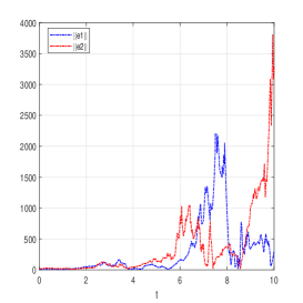
Figure 1: The error dynamic trajectory when $i=1,2$ without controller.

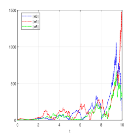
Figure 2: The error dynamic trajectory when $i=3,4,5$ without controller.

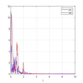
Figure 3: The error dynamic trajectory when $i=1,2$ with the pinning impulsive controllers (6).

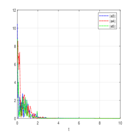
Figure 4: The error dynamic trajectory when $i=3,4,5$ with the pinning impulsive controllers (6).

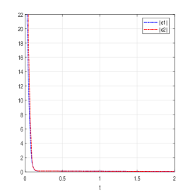
Figure 5: The error dynamic trajectory $i=1,2$ with the hybrid controllers (23).

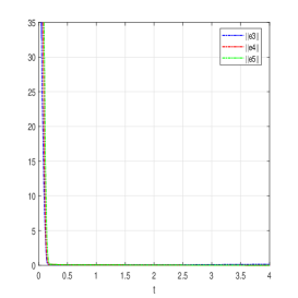
Figure 6: The error dynamic trajectory when $i=3,4,5$ with the hybrid controllers (23).

5 Conclusion

In this article, the problem concerning asymptotic and finite-time cluster synchronization of coupled neural networks with time-varying delay via two different control schemes is mainly concerned. First, we select some typical nodes in the coupling neural networks, and apply the control of pinning impulse [40] which can achieve the goal of saving control costs and is helpful to obtain sufficient conditions for asymptotic cluster synchronization of the systems. Second, motivated by the goal of pinning control method which is operated by precedence controlling some key nodes, we introduce the hybrid controllers to deal with finite-time synchronization of the error system. Third, we show a numerical example by exhibiting three cases to show the correctness and effectiveness.

Using the properties of fractional-order calculus and the research technique of fractional-order energy function, the influence of two control schemes on the asymptotic and finite-time cluster synchronization of the fractional-order coupled neural networks with time-varying delays is studied. The result will emerge in the near future. What’s more, complex-valued or quaternion-valued coupled neural networks with time-varying delays under the two control schemes in this paper have attracted the interest of many researchers. Hence, the future works also include asymptotic and finite-time cluster synchronization of complex-valued and quaternion-valued coupled neural networks with time-varying delays by pinning impulsive control and hybrid control.

References

- [1] J. Zha and C. Li. Synchronization of complex network based on the theory of gravitational field. Acta Physica Polonica B, 50(1):87–114, 2019.
- [2] J. Zhou, J. Chen, J. Lu, and J. Lu. On applicability of auxiliary system approach to detect generalized synchronization in complex network. IEEE Transactions on Automatic Control, 62(7):3468–3473, 2017.
- [3] S. Zhu, J. Zhou, X. Yu, and J. Lu. Bounded synchronization of heterogeneous complex dynamical networks: A unified approach. IEEE Transactions on Automatic Control, 66(4):1756–1762, 2020.
- [4] Z. Xu, P. Shi, H. Su, Z. Wu, and T. Huang. Global h∞ pinning synchronization of complex networks with sampled-data communications. IEEE Transactions on Neural Networks and Learning Systems, 29(5):1467–1476, 2018.
- [5] Y. Wu and L. Guo. Enhancement of intercellular electrical synchronization by conductive materials in cardiac tissue engineering. IEEE Transactions on Biomedical Engineering, 65(2):264–272, 2018.
- [6] F. Ren, F. Cao, and J. Cao. Mittag-leffler stability and generalized mittag-leffler stability of fractional-order gene regulatory networks. Neurocomputing, 160:185–190, 2015.
- [7] S. Kumar, R.and Sarkar, S. Das, and J. Cao. Projective synchronization of delayed neural networks with mismatched parameters and impulsive effects. IEEE Transactions on Neural Networks and Learning Systems, 31(4):1211–1221, 2020.
- [8] A. Abdurahman and H. Jiang. Improved control schemes for projective synchronization of delayed neural networks with unmatched coefficients. International Journal of Pattern Recognition and Artificial Intelligence, 34(3), 2020.
- [9] Adel O., X. Wang, V. Pham, and G. Giuseppe. Coexistence of identical synchronization, antiphase synchronization and inverse full state hybrid projective synchronization in different dimensional fractional-order chaotic systems. Advances in Difference Equations, 2018(1):1–16, 2018.
- [10] Q. Yang, H. Wu, and J. Cao. Global cluster synchronization in finite time for complex dynamical networks with hybrid couplings via aperiodically intermittent control. Optimal Control Applications and Methods, 41(4):1097–1117, 2020.
- [11] L. Liu, K. Liu, H. Xiang, and Q Liu. Cluster synchronization for directed complex dynamical networks via pinning control. Physica A: Statistical Mechanics and its Applications, 545:123580, 2020.
- [12] A. Hu, J. Cao, M. Hu, and L. Guo. Cluster synchronization of complex networks via event-triggered strategy under stochastic sampling. Complexity, 434:99–110, 2015.
- [13] Y. Wang, Z. Ma, J. Cao, and A. Alsaedi. Adaptive cluster synchronization in directed networks with nonidentical nonlinear dynamics. Complexity, 21:380–387, 2016.
- [14] W. Wu, W. Zhou, and T. Chen. Cluster synchronization of linearly coupled complex networks under pinning control. IEEE Transactions on Circuits and Systems, 56(4):829–839, 2009.
- [15] Q. Yang, H. Wu, and J. Cao. Global cluster synchronization in finite time for complex dynamical networks with hybrid couplings via aperiodically intermittent control. Optimal Control Applications and Methods, 41(4):1097–1117, 2020.
- [16] J. Cao, G. Chen, and P. Li. Generalized analytical solutions and experimental confirmation of complete synchronization in a class of mutually-coupled simple nonlinear electronic circuits. Nonlinear Sciences, 113:294–307, 2017.
- [17] A. Koronovskii, O. Moskalenko, V. Ponomarenko, M. Prokhorov, and A. Hramov. Binary generalized synchronization. Chaos Splitions and Fractals, 83:133–139, 2016.
- [18] D. Senthilkumar, M. Lakshmanan, and J. Kurths. Phase synchronization in unidirectionally coupled ikeda time-delay systems. Nonlinear Sciences, 164(11):35–44, 2008.
- [19] K. Li, J. Zhao, H. Zhang, and X. Li. On successive lag synchronization of a dynamical network with delayed couplings. IEEE Transactions on Control of Network Systems, page 1, 2021.
- [20] S. Yang, C. Hu, J. Yu, and H. Jiang. Finite-time cluster synchronization in complex-variable networks with fractional-order and nonlinear coupling. Neural networks: the official journal of the International Neural Network Society, 135:212–224, 2020.
- [21] S. Liu, N. Jiang, A. Zhao, Y. Zhang, and K. Qiu. Secure optical communication based on cluster chaos synchronization in semiconductor lasers network. IEEE Access, 8:11872–11879, 2020.
- [22] L. Pan, J. Cao, U. Al-Juboori, and M. Abdel-Aty. Cluster synchronization of stochastic neural networks with delay via pinning impulsive control. Neurocomputing, 366(13):109–117, 2019.
- [23] P. Liu, Z. Zeng, and J. Wang. Asymptotic and finite-time cluster synchronization of coupled fractional-order neural networks with time delay. IEEE Transactions on Neural Networks and Learning Systems, PP(99), 2020.
- [24] J. Mei, M. Jiang, W. Xu, and B. Wang. Finite-time synchronization control of complex dynamical networks with time delay. Communications in Nonlinear Science and Numerical Simulation, 18(9):2462–2478, 2013.
- [25] P. He, S. Ma, and T. Fan. Finite-time mixed outer synchronization of complex networks with coupling time-varying delay. Chaos, 22(4):175–423, 2012.
- [26] Z. Hou, Jun P., Z. Liu, J. Zou, and J. Luo. Theory of functional differential equations. Journal of Changsha Railway University, 2001.
- [27] X. Jin, Z. Wang, H. Yang, Q. Song, and M. Xiao. Synchronization of multiplex networks with stochastic perturbations via pinning adaptive control. Journal of the Franklin Institute, 2021.
- [28] S. Ding and Z. Wang. Synchronization of coupled neural networks via an event-dependent intermittent pinning control. IEEE Transactions on Systems, Man, and Cybernetics: Systems, pages 1–7, 2020.
- [29] W. Li, J. Zhou, J. Li, T. Xie, and J. Lu. Cluster synchronization of two-layer networks via aperiodically intermittent pinning control. IEEE Transactions on Circuits and Systems II: Express Briefs, page 1, 2020.
- [30] X. Li, D. Peng, and J. Cao. Lyapunov stability for impulsive systems via event-triggered impulsive control. IEEE Transactions on Automatic Control, 65(11):4908–4913, 2020.
- [31] X. Li, X. Yang, and J. Cao. Event-triggered impulsive control for nonlinear delay systems. Automatica, 117, 2020.
- [32] W. He, F. Qian, and J. Cao. Pinning-controlled synchronization of delayed neural networks with distributed-delay coupling via impulsive control. Neural Networks, 85:1–9, 2017.
- [33] X. Xiong, X. Yang, J. Cao, and R. Tang. Finite-time control for a class of hybrid systems via quantized intermittent control. Sci. China Inf. Sci., 63(9):192201, 2020.
- [34] S. Liu, Wu H., and J. Cao. Fixed‐time synchronization for discontinuous delayed complex‐valued networks with semi‐markovian switching and hybrid couplings via adaptive control. International Journal of Adaptive Control and Signal Processing, 34(10):1359–1382, 2020.
- [35] Z. Wu, Q. Ye, and D. Liu. Finite-time synchronization of dynamical networks coupled with complex-variable chaotic systems. 2013.
- [36] H. Wang, Z. Han, Q. Xie, and W. Zhang. Finite-time chaos control via nonsingular terminal sliding mode control. Communications in Nonlinear Science and Numerical Simulation, 14(6):2728–2733, 2009.
- [37] L. Liu and Q. Liu. Cluster synchronization in complex dynamical network of nonidentical nodes with delayed and non-delayed coupling via pinning control. Physica Scripta, 94(4), 2019.
- [38] X. Liu and T. Chen. Finite-time and fixed-time cluster synchronization with or without pinning control. IEEE Transactions on Cybernetics, 48(99):240–252, 2018.
- [39] Q. Wu, Z. Jin, and X. Lan. Global exponential stability of impulsive differential equations with any time delays. Applied Mathematics Letters, 23(2):143–147, 2010.
- [40] C. Aouiti, M. Bessifi, and X. Li. Finite-time and fixed-time synchronization of complex-valued recurrent neural networks with discontinuous activations and time-varying delays. Circuits Systems and Signal Processing, pages 1–23, 2020.