Monoceros OB4: a new association in Gaia DR2

Abstract

We use Gaia DR2 data to survey the classic Monoceros OB1 region and look for the existence of a dispersed young population, co-moving with the cloud complex. An analysis of the distribution of proper motions reveals a 20-30 Myr association of young stars, about 300-400 pc away from the far side of the Mon OB1 complex, along the same general line-of-sight. We characterize the new association, Monoceros OB4, and estimate it contains between 1400 and 2500 stars, assuming a standard IMF, putting it on par in size with NGC 2264. We find from the internal proper motions that Mon OB4 is unbound and expanding. Our results seem to unveil a larger and more complex Monoceros star formation region, suggesting an elongated arrangement that seems to be at least $300\times 60$ pc.

1 Introduction

Studies of star formation in the Milky Way has been traditionally focused on the densest star forming gas clumps. For the local clouds complexes we have today an essentially complete sample of embedded YSOs with ages of about 1 Myr, mostly found via space-based infrared missions. Almost paradoxically, little is known about the environs of star forming regions, which could contain more evolved YSOs with ages up to 10 Myr, mostly dust free and detectable at optical wavelengths. The existence, or absence, of an extended young optically visible population near active star forming-regions, is critical to establish their star formation history and could inform on the role of feedback in the star formation.

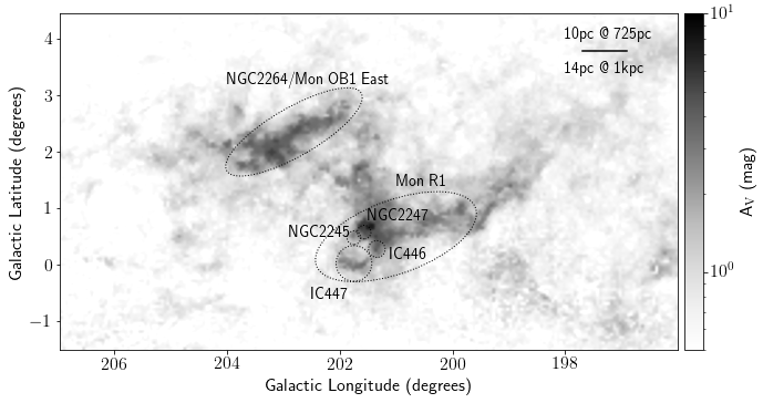
Figure 1: Dust extinction map of the Monoceros OB1 complex, integrated along the line-of-sight up to 1 kpc (Green et al., 2019). The most prominent star-forming region is NGC 2264; it is located within the ellipse representing the approximate area surveyed with Spitzer by Rapson et al. (2014). Other known star-forming regions, located in Mon R1 region, are marked by dashed circles (Bhadari et al., 2020). A scale bar is shown for reference.

This is the first of a series of papers on the stellar populations in Monoceros OB1, where we conduct a comprehensive wide-field survey to identify and characterize all the co-moving, coeval, and co-distant groups of sources. Monoceros OB1’s molecular cloud complex is located between 697 pc and 784 pc Zucker et al. (2019), and has spawned the NGC 2264 cluster in the east, and a series of reflection nebula (termed Mon R1 by van den Bergh, 1966) in the west (see Figure 1). The most well studied cluster in Mon OB1 is NGC 2264 (Dahm, 2008, and references therein),(Young et al., 2006; Teixeira et al., 2006, 2007; Teixeira et al., 2008; Forbrich et al., 2010; Alencar et al., 2010; Kwon et al., 2011; Teixeira et al., 2012; Mariñas et al., 2013; Pineda & Teixeira, 2013; Cody et al., 2014; Rapson et al., 2014; Venuti et al., 2014; McGinnis et al., 2015; Sousa et al., 2016; Tobin et al., 2015; Schneider et al., 2018; Costado & Alfaro, 2018; Venuti et al., 2019; Sousa et al., 2019; Montillaud et al., 2019b, a; Buckner et al., 2020; Jackson et al., 2020; Pearson et al., 2020). Mon R1 contains the less well characterized NGC 2245, NGC 2247, IC 446, and IC 447 young clusters (Glushkov, 1972; Dzhakusheva et al., 1988; Casey, 1991; Bhadari et al., 2020). We report on the discovery of a new cluster, comparable in size to NGC 2264, that is located behind the molecular clouds.

2 Gaia DR2 data quality filtering

We investigated Gaia DR 2 data (Gaia Collaboration et al., 2018; Lindegren et al., 2018) for the area shown in Figure 1, corresponding to 196.5° $<$ l $<$ 206.5° and 4.5° $<$ b $<$ -1.5°. These data were cross-matched, via the Gaia DR 2 source identification number, with the catalog of Bailer-Jones et al. (2018) that provides estimated distances, along with lower and upper bounds of the confidence interval of the estimated distances. We filtered the Gaia DR2 data by selecting sources (i) with parallax/parallax error, $\varpi/\sigma_{\varpi}$, greater than 10.0 and (ii) with errors in proper motion, $\sigma_{\mu_{\alpha}^{*}}$ and $\sigma_{\mu_{\delta}}$, less than 0.2 mas yr^-1.

3 Identification of the new co-moving group and selection of candidate members

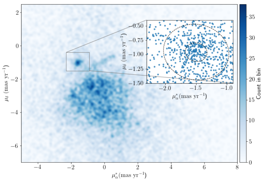
Figure 2: Gaia DR2 proper motion density map for sources within the area shown in Figure 1, that have estimated distances between 1000 and 1300 parsecs, and with the data quality filtering described in Section 2. The proper motion density colormap has a bin size of 0.08 mas yr^-1, Nyquist sampled. The plot shown in the inset contains the proper motions of the sources located within the box on the colormap; the 1- and 3-$\sigma$ contour levels of the fitted bivariate Gaussian are also shown within the inset plot.

We use a sub-sample of the Gaia DR2 filtered data (as described in Section 2), consisting of sources that have a lower bound of the estimated distance of 1000 pc and an upper bound of 1300 pc (analysis of other distance layers will be presented in future work). Figure 2 (a) shows the distribution of sources in this sub-sample in the proper motion space; the density map was built using a square bin of size 0.08 mas yr^-1, and is Nyquist sampled. The color map shows a well defined density peak, marked by the gray box. The proper motions of the sources that fall within the box are shown in the inset, where they are fit using robust parameter estimation of a bivariate Gaussian (Vanderplas et al., 2012; Ivezić et al., 2014); we retain sources whose proper motion fall within the 3-$\sigma$ contour level of the ellipse that is centered on ($\mu_{\alpha}^{*},\mu_{\delta}$)=(-1.5, -0.9)  mas yr^-1.

We used the same sub-sample of data to build a density map in the transverse velocity phase space. The transverse velocity along right ascension, $V_{\mathrm{T_{\alpha}}}$, and declination, $V_{\mathrm{T_{\delta}}}$, are given by:

$$V_{\mathrm{T_{\alpha}}}^{*}=4.74\mu_{\alpha}^{*}d=4.74\mu_{\alpha}cos(\delta)d,$$ (1)

$$V_{\mathrm{T_{\delta}}}=4.74\mu_{\delta}d,$$ (2)

where $d$ corresponds to the estimated distance to the source given in pc, the proper motions are given in ″yr^-1, and the transverse velocities are calculated in  km s^-1. The transverse velocity density map was built using a square bin of size 0.37 km s^-1, Nyquist sampled. We retained sources within the 3-$\sigma$ contour level of the bivariate Gaussian, in the respective proper motion and transverse velocities phase spaces, as a first selection criteria for members of the new co-moving group. Table 1 summarizes the parameters of the 3-$\sigma$ ellipses, including the rotation angles for the proper motion ($\theta_{\mu}$) and transverse velocity ($\theta_{V_{T}}$). We selected sources that satisfied both $\mu$ and $V_{\mathrm{T}}$ criteria simultaneously, in order to minimize contamination. We expanded the search for candidate members, with the above kinematic criteria, for distances down to 400 pc, in order to compare with the known population of Mon OB1 and to account for the large distance uncertainties. The new co-moving group has 242 candidate members (listed in Table 2), and is located at a mean distance of 1182 $\pm$122 pc. We show in panel (a) of Figure 3 the spatial distribution of the co-moving group in comparison to the molecular clouds in the Mon OB1 complex. We calculate the median values of coordinates of the candidate members and find the center of the co-moving group to be $(l,b)$=(202.2°,1.1°), with an estimated radius of 0.5°. We should note that since the co-moving group is located behind the molecular cloud complex, we are missing those members that are too extincted to be detected by Gaia, and as such the actual co-moving group center may be shifted to the west.

Table 1: Kinematic selection criteria.

$\mu_{\alpha}^{*}\pm 3\sigma_{\mu_{\alpha}^{*}}$ = -1.52 $\pm$ 0.47  mas yr-1	$V_{\mathrm{T_{\alpha}}}^{*}\pm 3\sigma_{V_{\mathrm{T_{\alpha}}}^{*}}$ = -6.47 $\pm$ 1.23  km s-1
$\mu_{\delta}\pm 3\sigma_{\mu_{\delta}}$ = -0.96 $\pm$ 0.39  mas yr-1	$V_{\mathrm{T}_{\delta}}\pm 3\sigma_{V_{\mathrm{T_{\delta}}}}$ = -3.80 $\pm$ 0.99  km s-1
$\theta_{\mu}$ = -0.24°	$\theta_{V_{\mathrm{T}}}$ = 1.35°

Table 2: List of candidate members of the new cluster. The full catalog will be available online.

Gaia DR2 Source ID	l (deg)	b (deg)	Dist. (pc)	Av (mag)
3369260560768525056	196.187	2.147	1076	0.6
3357029833938241024	197.528	3.583	1165	0.6
3356941666849693568	197.588	2.670	1275	1.1
3356860921465018240	196.439	1.815	1201	0.6
3356834975564998784	196.489	1.639	1043	0.7

4 Age and mass function

Figure 4 shows the de-reddened Gaia DR2 color-magnitude diagram. We use the Bayestar dust extinction map (Green et al., 2019), to estimate the individual extinction for each source. According to this method, the sources have an average extinction of A${}_{\mathrm{V}}={1.0}\pm 0.5$ mag. We determine an approximate age between 20 and 30 Myr. Spectroscopic follow-up observations are needed to obtain spectral types and more exact extinction measurements to determine a more precise age for the new group. We note that several other factors also contribute to a spread in the distribution of the sources in the color-magnitude diagram, such as binarity, distance uncertainties, and stellar variability (Jeffries et al., 2011).

Using the de-reddened color-magnitude diagram, and the MIST mass tracks (Choi et al., 2016; Dotter, 2016), we estimate individual stellar masses and built the mass function shown in Figure 5. In order to estimate the total mass of the new co-moving group, we generated clusters of different total masses, using the Kroupa (2001) initial mass function (IMF), and the publicly available python package imf. We show in Figure 5  the IMFs of these simulated clusters, with total masses ranging from 600 M_⊙ to 3000 M_⊙, and show that the total mass of the new co-moving group is estimated to be between 600 and 1200 M_⊙ (containing between 1400 and 2500 stars). We remind the reader that, since the new group is located behind the molecular cloud complex, we are missing those members that are too extincted to be detected by Gaia DR2. For comparison, regarding the population of NGC 2264, Teixeira et al. (2012) calculated a total number of sources of 1436 $\pm$ 242, while (Buckner et al., 2020) estimate a population of 1795 (differences in the areas surveyed and the wavelength coverage may account for the slightly differing values). The new co-moving group is therefore comparable in population size to NGC 2264. We henceforth refer to the new co-moving group as the Monoceros OB4 association.

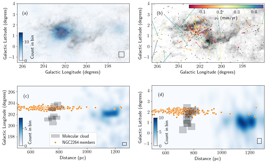
Figure 3: 3D spatial representation of the new association Mon OB4. Panel (a) shows the $(l.b)$ spatial density (blue colorscale) overplotted on the dust map (c.f. Figure 1). Panel (b) shows

the $(l.b)$ spatial distribution of the candidate members ( black points) overplotted on the dust map, with the vectors representing their proper motion relative to the mean of Mon OB4. Panels (c) and (d) show the Mon OB4 density distribution of $l$ and $b$, respectively, as a function of distance (blue colormap). Also represented are the Mon OB1 molecular clouds (gray boxes) and NGC 2264 members (Venuti et al., 2014) (orange points). The distances to the clouds are taken from Zucker et al. (2019); cloud depths are as yet unknown and we take a value of 50 pc for schematic purposes. The bottom left rectangle in panels (a), (c), and (d) correspond to the pixel size of the respective density map (20 pc for distance and 0.5° for $l$ and $b$).

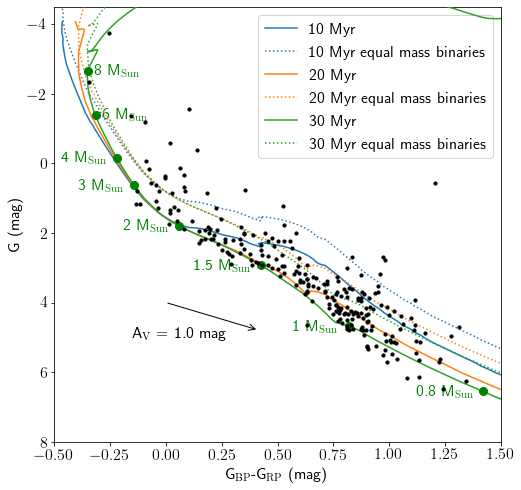
Figure 4: Color-magnitude diagram for the sources in the co-moving group, with overplotted MIST isochrones (Choi et al., 2016; Dotter, 2016) for single stars (solid lines) and equal-mass binaries (dotted lines) for 30, 20, and 10 Myr (green, orange, and blue, respectively)

.

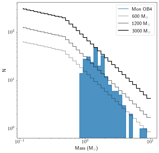
Figure 5: Present day mass function of the Mon OB4 (solid histogram). For comparison, we over plot the initial mass functions of simulated clusters of total masses ranging between 600 M_⊙ and 3000 M_⊙ (open histograms).

5 Discussion

5.1 2D kinematic structure: expansion

We transformed the proper motions from the ICRS ($\alpha,\delta$) plane to the Galactic ($l,b$) plane, and subtracted the mean proper motion values of Mon OB4, ($\mu_{l},\mu_{b}$) = (0.09, -1.80) mas yr^-1 from the individual sources in order to ascertain their relative motions. Panel (b) of Figure 3 shows these relative proper motion vectors, color-coded by their value. To simplify the diagram, we show only the vectors for the brightest sources, with G $<$ 2.5 mag. As can be seen, the proper motion value is correlated with the distance of the source to the center of Mon OB4: sources located closest to the center have lower proper motions, while sources located further away have larger proper motions. This is a classic signature of an expanding cluster, also observed in $\lambda$ Orionis (Kounkel et al., 2018), and modeled by Arnold & Goodwin (2019). We do note however, that due to the lack of radial velocity information we are unable to correct for virtual expansion (Brown et al., 1997).

The virial mass of a cluster is given by (Mihalas & Routly, 1968):

$$M=466<R><v^{2}>,$$ (3)

where $<R>$ is the mean distance between the stars in pc, $<v^{2}>$ is the square of the dispersion of space velocities in  km s^-1. To calculate the virial mass of the cluster, we create a sub-sample corresponding to the region where the stellar density is greater than 5-$\sigma$, which corresponds to the following box: 202.53° $<l<$ 201.78°, 1.39° $<b<$ 0.74°. For this sub-sample, $<R>$ = 4.4 pc and $<v^{2}>$ = 1.1 km s^-1 (in the absence of radial velocities we assume isotropy). We calculate a virial mass of 2364 M_⊙, which is greater than the total estimated mass of Mon OB4 association (by a factor of two, at least). This is a first rough estimate for the current data (keeping in mind the aforementioned caveats such as missing sources that are too extincted for Gaia DR2 detection, velocity isotropy), suggesting that Mon OB4 is unbound, which is in agreement with the expansion signature described above and seen in Figure 3 panel (a).

5.2 3D spatial distribution

We carried out an analysis of the maximum likelihood in the 3D multivariate Gaussian space of parallax and proper motion (Lindegren et al., 2000; Roccatagliata et al., 2020), to explore whether sources located at $l<$ 200° (farthest from the center of Mon OB4, on the plane-of-the-sky) could be part of a different population, but we found no statistically significant difference. The population is consistent with a single peak in the parallax and proper motion space. Figure 3 shows the distribution of Mon OB4 in Galactic Longitude and Latitude coordinates as a function of distance in panels (c) and (d), respectively. Also shown for comparison purposes are the clouds (distances taken from Zucker et al., 2019) and the NGC 2264 cluster (spectroscopically confirmed members taken from Venuti et al., 2014). At first glance, the distance between the new Mon OB4 association and the Mon OB1 star-forming clouds, $\sim$400 pc, seems too large for these two structures to be physically connected. Stassun & Torres (2018) found a systematic offset in the parallaxes reported in Gaia DR2 of -82 $\pm$ 33 $\mu$as. At a distance of 1183 pc, this corresponds to an average distance overestimation of 105 pc bringing the distance of the new association Mon OB4 to 1078 pc, and reducing the separation to the clouds to $\sim$300 pc. A careful Gaia DR2 analysis of the Taurus star-forming region has revealed that the complex has a depth of 200 pc (Roccatagliata et al., 2020). Presumably more massive regions would span larger depths, so it is not entirely unfeasible that Mon OB4 could be associated with the star-forming complex in Mon OB1. For example, Chen et al. (2019), also using Gaia DR2 data, found that the young stellar population in the large Orion star forming region extends for about 300 pc, with ages spanning 0-20 Myr, similar to our results in Mon OB1. Finally, Alves et al. (2020) found that the location of the large majority of the local star forming regions is not random but highly correlated. In particular, they found an undulating 2.7 kpc structure, the Radcliffe Wave, likely associated with the Local Arm of the Galaxy, containing all the major local star forming regions from Canis Major to Cygnus. Monoceros OB1 is not part of the Radcliffe Wave (see their interactive Figure 2), but the extended configuration of Mon OB1 proposed here is not surprising in the context of the spatial distribution of star formation in the Local Neighborhood. It is suggestive, on the other hand, of a possible connection between Mon OB1 and the Rosette nebula, at 1.6 kpc (c.f. Cepheus Spur, Pantaleoni González et al., 2021). Although it is likely that the new population presented in this Letter is associated with the star formation event that formed NGC 2264, radial velocity data are needed to further investigate and confirm this scenario, by determining how the new Mon OB4 association and clusters emerging from the clouds (e.g. NGC 2264 and IC 447) are moving with respect to each other in 3D.

6 Summary of conclusions

We report on the discovery of a new co-moving group of young sources in Monoceros, also independently identified by Kounkel & Covey (2019); Kounkel et al. (2020). We name the new group as the Monoceros OB4 association; it is comparable in estimated population size to NGC 2264, and with the following characteristics:

• its central coordinates are $(l,b)$ = (202.2°, 1.1°);

• its mean proper motion is given by ($\mu_{\alpha}^{*},\mu_{\delta}$) = (-1.52, -09.6)  mas yr^-1;

• it is located at a distance of $\sim$1 kpc, placing it behind the molecular clouds associated with Mon OB1 East (NGC 2264) and Mon OB1 West (NGC 2245, NGC 2247, IC 446 and IC 447);

• its age is estimated to be between 20 and 30 Myr;

• it has a total mass estimate between 600 and 1200 M_⊙and between 1400 and 2500 sources;

• it is unbound and appears to be expanding;

• Our results seem to unveil a larger and more complex Monoceros star formation region, suggesting an elongated arrangement that seems to be at least $300\times 60$ pc.

Radial velocity observations are needed to further investigate the motion of the new population in 3D with respect to the clusters associated with the molecular cloud complex.

7 Data availability

The data underlying this article will be made available in http://cdsarc.u-strasbg.fr/

References

- Alencar et al. (2010) Alencar S. H. P., et al., 2010, A&A, 519, A88
- Alves et al. (2020) Alves J., et al., 2020, Nature, 578, 237
- Arnold & Goodwin (2019) Arnold B., Goodwin S. P., 2019, MNRAS, 483, 3894
- Astropy Collaboration et al. (2013) Astropy Collaboration et al., 2013, Astronomy and Astrophysics, 558, A33
- Bailer-Jones (2015) Bailer-Jones C. A. L., 2015, PASP, 127, 994
- Bailer-Jones et al. (2018) Bailer-Jones C. A. L., Rybizki J., Fouesneau M., Mantelet G., Andrae R., 2018, The Astronomical Journal, 156, 58
- Bhadari et al. (2020) Bhadari N. K., Dewangan L. K., Pirogov L. E., Ojha D. K., 2020, arXiv e-prints, p. arXiv:2006.13894
- Brown et al. (1997) Brown A. G. A., Dekker G., de Zeeuw P. T., 1997, MNRAS, 285, 479
- Buckner et al. (2020) Buckner A. S. M., et al., 2020, A&A, 636, A80
- Casey (1991) Casey S. C., 1991, ApJ, 371, 183
- Chen et al. (2019) Chen B., D’Onghia E., Alves J., Adamo A., 2019, arXiv e-prints, p. arXiv:1905.11429
- Choi et al. (2016) Choi J., Dotter A., Conroy C., Cantiello M., Paxton B., Johnson B. D., 2016, ApJ, 823, 102
- Cody et al. (2014) Cody A. M., et al., 2014, AJ, 147, 82
- Costado & Alfaro (2018) Costado M. T., Alfaro E. J., 2018, MNRAS, 476, 3160
- Dahm (2008) Dahm S. E., 2008, The Young Cluster and Star Forming Region NGC 2264. p. 966
- Dotter (2016) Dotter A., 2016, ApJS, 222, 8
- Dzhakusheva et al. (1988) Dzhakusheva K. G., Kuratov K. S., Mukanov D. B., Bergner Y. K., Miroshnichenko A. S., Yudin R. V., Ytanov N. Y., 1988, Pisma v Astronomicheskii Zhurnal, 14, 744
- Forbrich et al. (2010) Forbrich J., Tappe A., Robitaille T., Muench A. A., Teixeira P. S., Lada E. A., Stolte A., Lada C. J., 2010, ApJ, 716, 1453
- Gaia Collaboration et al. (2018) Gaia Collaboration et al., 2018, Astronomy and Astrophysics, 616, A1
- Glushkov (1972) Glushkov Y. I., 1972, Astronomicheskij Tsirkulyar, 692, 1
- Green et al. (2019) Green G. M., Schlafly E., Zucker C., Speagle J. S., Finkbeiner D., 2019, ApJ, 887, 93
- Hunter (2007) Hunter J. D., 2007, Computing in Science and Engineering, 9, 90
- Ivezić et al. (2014) Ivezić Ž., Connolly A., Vanderplas J., Gray A., 2014, Statistics, Data Mining and Machine Learning in Astronomy. Princeton University Press
- Jackson et al. (2020) Jackson R. J., et al., 2020, MNRAS, 496, 4701
- Jeffries et al. (2011) Jeffries R. D., Littlefair S. P., Naylor T., Mayne N. J., 2011, MNRAS, 418, 1948
- Kounkel & Covey (2019) Kounkel M., Covey K., 2019, AJ, 158, 122
- Kounkel et al. (2018) Kounkel M., et al., 2018, AJ, 156, 84
- Kounkel et al. (2020) Kounkel M., Covey K., Stassun K. G., 2020, AJ, 160, 279
- Kroupa (2001) Kroupa P., 2001, MNRAS, 322, 231
- Kwon et al. (2011) Kwon J., et al., 2011, ApJ, 741, 35
- Lindegren et al. (2000) Lindegren L., Madsen S., Dravins D., 2000, A&A, 356, 1119
- Lindegren et al. (2018) Lindegren L., et al., 2018, Astronomy and Astrophysics, 616, A2
- Mariñas et al. (2013) Mariñas N., Lada E. A., Teixeira P. S., Lada C. J., 2013, ApJ, 772, 81
- McGinnis et al. (2015) McGinnis P. T., et al., 2015, A&A, 577, A11
- Mihalas & Routly (1968) Mihalas D., Routly P. M., 1968, Galactic astronomy
- Montillaud et al. (2019a) Montillaud J., et al., 2019a, A&A, 631, A3
- Montillaud et al. (2019b) Montillaud J., et al., 2019b, A&A, 631, L1
- Pantaleoni González et al. (2021) Pantaleoni González M., Maíz Apellániz J., Barbá R. H., Reed B. C., 2021, arXiv e-prints, p. arXiv:2103.02748
- Pearson et al. (2020) Pearson S., Scholz A., Teixeira P. S., Mužić K., Eislöffel J., 2020, MNRAS, 499, 2292
- Pineda & Teixeira (2013) Pineda J. E., Teixeira P. S., 2013, A&A, 555, A106
- Rapson et al. (2014) Rapson V. A., Pipher J. L., Gutermuth R. A., Megeath S. T., Allen T. S., Myers P. C., Allen L. E., 2014, ApJ, 794, 124
- Robitaille & Bressert (2012) Robitaille T., Bressert E., 2012, Astrophysics Source Code Library, p. ascl:1208.017
- Roccatagliata et al. (2020) Roccatagliata V., Franciosini E., Sacco G. G., Rand ich S., Sicilia-Aguilar A., 2020, A&A, 638, A85
- Schneider et al. (2018) Schneider P. C., Manara C. F., Facchini S., Günther H. M., Herczeg G. J., Fedele D., Teixeira P. S., 2018, A&A, 614, A108
- Sousa et al. (2016) Sousa A. P., et al., 2016, A&A, 586, A47
- Sousa et al. (2019) Sousa A. P., Alencar S. H. P., Rebull L. M., Espaillat C. C., Calvet N., Teixeira P. S., 2019, A&A, 629, A67
- Stassun & Torres (2018) Stassun K. G., Torres G., 2018, ApJ, 862, 61
- Taylor (2005) Taylor M. B., 2005, Astronomical Data Analysis Software and Systems XIV ASP Conference Series, 347, 29
- Teixeira et al. (2006) Teixeira P. S., et al., 2006, ApJ, 636, L45
- Teixeira et al. (2007) Teixeira P. S., Zapata L. A., Lada C. J., 2007, ApJ, 667, L179
- Teixeira et al. (2008) Teixeira P. S., McCoey C., Fich M., Lada C. J., 2008, MNRAS, 384, 71
- Teixeira et al. (2012) Teixeira P. S., Lada C. J., Marengo M., Lada E. A., 2012, A&A, 540, A83
- Tobin et al. (2015) Tobin J. J., Hartmann L., Fűrész G., Hsu W.-H., Mateo M., 2015, AJ, 149, 119
- Vanderplas et al. (2012) Vanderplas J., Connolly A., Ivezić Ž., Gray A., 2012, in Conference on Intelligent Data Understanding (CIDU). pp 47 –54, doi:10.1109/CIDU.2012.6382200
- Venuti et al. (2014) Venuti L., et al., 2014, A&A, 570, A82
- Venuti et al. (2019) Venuti L., Damiani F., Prisinzano L., 2019, A&A, 621, A14
- Young et al. (2006) Young E. T., et al., 2006, ApJ, 642, 972
- Zucker et al. (2019) Zucker C., Speagle J. S., Schlafly E. F., Green G. M., Finkbeiner D. P., Goodman A. A., Alves J., 2019, The Astrophysical Journal, 879, 125
- van den Bergh (1966) van den Bergh S., 1966, AJ, 71, 990
- van der Walt et al. (2011) van der Walt S., Colbert S. C., Varoquaux G., 2011, Computing in Science and Engineering, 13, 22