Visual Place Recognition using LiDAR Intensity Information

Abstract

Robots and autonomous systems need to know where they are within a map to navigate effectively. Thus, simultaneous localization and mapping or SLAM is a common building block of robot navigation systems. When building a map via a SLAM system, robots need to re-recognize places to find loop closure and reduce the odometry drift. Image-based place recognition received a lot of attention in computer vision, and in this work, we investigate how such approaches can be used for 3D LiDAR data. Recent LiDAR sensors produce high-resolution 3D scans in combination with comparably stable intensity measurements. Through a cylindrical projection, we can turn this information into a panoramic image. As a result, we can apply techniques from visual place recognition to LiDAR intensity data. The question of how well this approach works in practice has not been answered so far. This paper provides an analysis of how such visual techniques can be with LiDAR data, and we provide an evaluation on different datasets. Our results suggest that this form of place recognition is possible and an effective means for determining loop closures.

I Introduction

Robots need to perceive their surroundings to navigate safely and act effectively. LiDAR sensors are a common sensor platform in robotics for several decades. Pushed by the increased safety required by the autonomous driving industry, 3D-LiDAR technology rapidly evolved in recent years. This resulted in having 3D instead of 2D sensing, fast and high-resolution point cloud acquisition, and intensity information for every 3D point – all at a rather low cost.

Figure 1: Today’s 3D-LiDARs measure both, the range and the intensity of the light reflected by the surrounding obstacles. Top: Example pairs of a query and a reference intensity image from our self-recorded dataset (IPB Car). Note that due to its high horizontal resolution (original size: $64\times 1024$), the intensity image has been divided in two parts, one above the other. The green line illustrate descriptor matches provided by HBST [34] on intenisty data. Bottom: The Newer College [31] (left) and IPB car (right) datasets used for evaluation, valid loop closures using HBST highlighted in green.

Vehicles use LiDARs to track their ego-motion as well as their surroundings and to build point cloud maps of the scene. Most vehicles focus on the 3D information and rely on the well-known graph-based Simultaneous Localization and Mapping (SLAM) paradigm to build maps. In this approach, the map of the environment is implicitly represented by the vehicle’s trajectory, with point clouds or local maps attached to trajectory nodes. A graph-based SLAM system works by constructing a SLAM graph where each node represents a robot position, while edges encode a relative displacement between nodes. These local transformations are inferred by comparing and matching nearby sensor readings. Edges between subsequent robot positions can be straightforwardly estimated by registering point clouds incrementally [24, 44]. Relocalization events or so-called loop closures, occurring when the robot reenters in a known location after a long travel. The events should trigger the creation of loop-closing edges, which are crucial to eliminate odometry drift and compute a globally consistent map. Finding such loop closures, however, can be challenging, especially in repetitive environments.

Existing 3D-LiDAR SLAM systems deliver accurate maps and yield real-time performance on standard computers. Still, a non-negligible number of approaches does not detect loops [46, 47, 10, 8], or rely on rather costly operations to check for candidate loop closures [4] – e.g., ICP in combination with outlier rejection mechanisms. This is because detecting loop-closures efficiently using only LiDAR data is still a challenge. Recently, learning-based techniques [6] became popular as well. In the context of camera images, however, this task is framed as Visual Place Recognition (VPR) and effective solutions exist [22, 43, 27]. In this paper, we investigate how such visual techniques can be applied to LiDAR scans, especially the reflected intensity data, in an easy manner and how effective such an approach is. An example of the application of VPR approaches to LiDAR intensity cues is depicted in Fig. 1.

The main contribution of this paper is an analysis that evaluates how existing visual place recognition techniques perform when applied to the intensity cue of a 3D LiDAR scanner. Thus, this paper is an experimental analysis and does not propose a new method to loop closing in general. We tested several variants of VPR pipelines in this context on multiple robotic datasets using 3D LiDARs. Our experiments show that the straightforward adaptation of existing VPR techniques can produce reliable loop closures, enabling laser-only LiDAR SLAM at large scales.

II Related Work

The early loop-closures detection systems for 3D scans extracted features from the raw data. Several feature extractors have been proposed, each capturing some traits of a local neighborhood of the scene. Early studies in this direction were made by Johnson [18] and later by Huber [17]. The former extracted some local 3D features from local point cloud patches, describing the local surface around points with orientation. The latter built on top of Johnson’s Spin Images a methodology to perform global registration exploiting these features. In this sense, each query frame is compared with a database, and if the surfaces of the local descriptors are “similar” between query and reference, then a potential loop-closure is detected. Steder et al. [36] investigated novel point features that are extracted directly from range images, and later, they applied them in the context of loop-closures detection [35]. Finally, Steder et al. proposed to use more robust NARF features [38] together with Bag-of-Words-based search to increase the efficiency and the accuracy of the detection [37]. Orthogonally, Magnusson et al. investigated the use of Normal Distributed Transform (NDT) as features to match 3D scans [23]. This approach has been originally developed to perform registration between scans; still, the authors demonstrated that NDT-based features capture enough structure to be used in the context of place recognition. Röhling et al. [32] investigated the use of histograms computed directly from the 3D point cloud to define a measure of the similarity of two scans. Novel types of descriptors have been investigated, exploiting additional data gathered by the LiDAR sensor – i.e., light remission of the beams [7, 16]. However, despite being very attractive, these descriptors are time-consuming to extract and match, resulting in a slower system overall.

More recently, deep learning approaches are spreading thanks to the increased computing power of today’s computers. Dubé et al. [13] proposed the detection and matching of segments to recognize whether we are observing an already visited place. Uy et al. [40] employed a CNN based on PointNet [29] to compute NetVLAD holistic descriptors [1] out of range images. Zaganidis et al. [45] used semantic information extracted from the point cloud [30] to enrich NDT features, resulting in more accurate and robust place recognition. Chen et al. [6], instead, developed and end-to-end solution to evaluate the overlap of two 3D scans together with a raw estimate of the yaw angle. Still, all deep-learning-based approaches require a great amount of data to perform training (most of the times also labeled) and a lot of computing power to work properly.

A lot of visual place recognition systems exploit features such as SURF [2] or SIFT [21] and several approaches apply bag-of-words techniques, i.e., they perform matching based on the appearance statistics of such features. To improve the robustness of appearance-based place recognition, Stumm et al. [39] consider the constellations of visual words and keeping track of their covisibility. Another popular approach for visual place recognition proposed by Galvez-Lopez et al. [14] proposes a bag of words approach using binary features for fast image retrieval. Single image visual localization in real-world outdoor environments is still an active field of research, and one popular approach used in robotics is FAB-MAP2 [9]. For across season matching using SIFT and SURF, Valgren and Lilienthal [41] propose to combine features and geometric constraints to improve the matching.

To deal with substantial variations in the visual input, it is useful to exploit sequence information for the alignment, compare [20, 25, 26, 27, 42, 43]. SeqSLAM [26] aims at matching image sequences under seasonal changes and computes a matching matrix that stores the similarity between the images in a query sequence and a database. Milford et al. [25] present a comprehensive study about the SeqSLAM performance on low-resolution images. Related to that, Naseer et al. [27] focus on sequence matching using a network flow approach and Vysotska et al. [42] extended this idea towards an online approach with lazy data association and build up a data association graph online on-demand, also allowing flexible trajectories in a follow-up work [43].

In this paper, we investigate how to perform fast and accurate place-recognition using additional channels available in modern 3D-LiDAR sensors. Our approach applies well-known methodologies originally designed to work with camera images to 3D-LiDARs data, exploiting the increased the descriptiveness of such sensors. We perform multiple experiments with different combinations of features - image retrieval tools. Among the features, we picked computationally efficient binary ones like BRISK [19] and ORB [33]. Instead, as floating point descriptors, we selected SURF [2] and Superpoint, a more recent neural extractor that shows impressive results compared to older geometrical features [11]. Among image-retrieval tools, we use HBST [34], a tree-like structure that allows for descriptor search and insertion in logarithmic time by exploiting particular properties of binary feature descriptors, and DBoW2 [14] that allows fast image retrieval based on the histogram of the distribution of words appearing in the image both for floating point and binary descriptors.

III LiDAR Sensors in Robotics

A typical LiDAR sensor emits a beam of pulsed light waves towards the measurement direction. The distance to the obstacle along the beam is measured from the light pulse’s round trip time. At a low level, a LiDAR senses the perceived light intensity $I_{r}(\rho,\lambda)$ as a function of the range of the reflection $\rho$ and the wavelength $\lambda$. The sensed intensity depends on the emitted intensity $I_{0}(\lambda)$ at the same wavelength, as follows:

$$I_{r}(\rho,\lambda)=I_{0}\eta\frac{A}{4\pi\rho^{2}}\beta(\rho,\lambda)\exp\left(-2\int_{0}^{\rho}\sigma(r,\lambda)\;dr\right).$$ (1)

Here, $A$ denotes the beam aperture measured as a solid angle, $\beta$ is the reflectance of the object, and $\sigma$ is the absorption of the medium. Fig. 2 illustrates this aspect. The reflectivity $\beta$ is affected by the composition, roughness and moisture content and incidence angle of the beam hitting the surface.

The resolution of the clock measuring the first return of the signal bounds the range measurement’s resolution. Additional accuracy gains, however, can be obtained by determining the phase difference between the emitted and received signal. A single detection can also be rather noisy. Therefore, scanners targeting higher accuracies send multiple pulses. This, in turn, caps the frequency of range measurements. The measurement frequency $f_{m}$ of a single sensor nowadays might reach 50 kHz. By choosing the rotation frequency $f_{r}$ of the beam, the angular resolution is straightforwardly $2\pi\frac{f_{m}}{f_{r}}$.

Figure 2: Illustration of a single beam emitting and receiving light pulse, as described in Eq. (1).

Mechanical considerations limit the rotational speed of the sensor. Whereas in the 2D case, the beam can be deflected by a relatively small rotating mirror, the sensor head carries multiple measuring units in the 3D case – today up to 128.

Scanners also measure the intensity of measurements as the amount of light reflected from the surface. This intensity information is normalized and discretized to an 8 or 16 bit value. The intensity depends on surface characteristics, and several other factors impact the measurement. All terms in Eq. (1) are continuous. Thus, we can expect that mild changes of the viewpoint yield mild variations of the intensity when measuring the same 3D point.

The majority of prior works on 3D-LiDARs for SLAM and place recognition focused on using the range measurements and ignored other potentially valuable information [47, 12]. This may also be since the intensity information of older scanners used in robotics was not as great. Compared to their predecessors, however, recent 3D-LiDARs exhibit an increased accuracy and vertical resolution. When assembled in a panoramic image, the intensity recalls the one obtained by using a grayscale camera. Undoubtedly, the quality of a LiDAR intensity image is still low compared to the one acquired by passive sensors such as cameras. However, in robotics and specifically in VPR tasks, the intensity image generated from a 3D-LiDAR scan brings advantages such as invariance to external light conditions and shadows.

The popularity of autonomous driving and self-driving cars pushed the improvement of 3D-LiDARs. In this application domain, their main use is to provide local 3D reconstruction and obstacle information. Traditionally, global 3D reconstruction using LiDARs presents a significant challenge of loop-closing. This arises from the higher sensor aliasing between range only 3D scans, compared to more descriptive images. The literature is rich in registration and mapping algorithms for 3D-LiDARs, whereas this community invested less effort in tasks such as place recognition, which forms the basis for effective loop closing. In contrast, the computer vision community invested substantial efforts in this place recognition task achieving impressive results [22]. Therefore, the purpose of this paper is to analyze the behavior of common VPR approaches when used in combination with LiDAR intensity information.

IV Visual Place Recognition Applied
to Cylindrical LiDAR Intensity Images

Popular VPR approaches often store a database of places in the form of a collection of image keypoints and descriptors (and potentially a coordinate in some world frame). The keypoints are salient points in the image, possibly corners and edges, while the descriptors encode the appearances around keypoints.

In the process of finding similar places, two images are regarded as similar if a substantial part of their keypoints’ descriptors are close to each other. Performing VPR using this paradigm requires first to convert a query image into a set of keypoints and descriptors and second to efficiently find images with similar descriptors. Effective solutions are available to quickly find the potential matches in the database, see [22]. Among all, we focus specifically on HBST [34] and DBoW2 [14] as two promitent approaches.

An intensity image constructed from a laser scan has a number of rows equal to the number of vertical beams and a number of columns equal to the number of scanning steps along the azimuth. Unfortunately, most public datasets provide the scans as annotated point clouds, and recovering the beam measurements needed for image formation requires a cylindrical projection. Due to vehicle motion, round-offs, or unknown parameters, this projection will likely result in missing data in some parts of the image. These phenomena may hinder the straightforward feature extraction process.

In the following, we will first discuss how we handle image formation from a laser scan, and then we review the structure of a straightforward pipeline for VPR.

IV-A Image Formation

When data of the raw beam measurements are not available given the scanner setup or given the dataset, we can compute a cylindrical image from the 3D point cloud $\mathcal{P}_{\mathrm{lid}}$ by spherical projection: $\Pi:\mathbb{R}^{3}\mapsto\mathbb{R}^{2}$. This is done by converting each Cartesian point $\mathbf{p}=\left(x,y,z\right)^{\top}\in\mathcal{P}_{\mathrm{lid}}$ as a spherical one $\bar{\mathbf{p}}=\left(\rho,\theta,\phi\right)^{\top}$, with:

$$\rho =\sqrt{x^{2}+y^{2}+z^{2}}$$

$$\theta =\operatorname*{atan2}(y,x)\in\left[-\pi/2,\pi/2\right]$$

$$\phi =\operatorname*{asin}(z/\rho)\in\left[-\pi,\pi\right].$$

Assuming that the beams are uniformly spaced over $f$, we can compute $\left(u,v\right)^{\top}$ as follows:

$$\begin{pmatrix}u\\ v\end{pmatrix}=\begin{pmatrix}\frac{W}{2}\left(1+\frac{\theta}{\pi}\right)\\ H\frac{f_{\mathrm{up}}-\phi}{f_{\mathrm{up}}-f_{\mathrm{low}}}\end{pmatrix},$$ (2)

where $W$ and $H$ are respectively the width and height of the image and $f=f_{\mathrm{up}}+f_{\mathrm{down}}$ is the vertical FoV of the sensor. Should multiple points fall in the same image pixel, only the value having the smallest range is retained. In each pixel of the created image, we store the intensity value and not the range.

The uneven distribution of the vertical beams may lead to empty gaps in the resulting image, usually whole horizontal rows. This problem can be solved a posteriori by either scaling down the vertical resolution or by performing interpolation. In the experiments on this paper, we adopted the second method. To remove the empty rows from a panoramic image, we first detect them using a binary threshold and a horizontal kernel as wide as the image. We compute the interpolated value for each pixel in the empty rows through bilinear interpolation based on the upper and lower valid rows’ values. Fig. 3 shows the result of this procedure.

Figure 3: Empty lines removal. From top to bottom, original image after projection from 3D point cloud as explained in Sec. IV-A, detection of empty rows highlighted in red, result after image manipulation. Each image shown has been cropped to half of their horizontal size for better viewing.

IV-B Feature Extraction

As stated at the beginning of this section, the feature extraction process aims at compressing an image in a set of interest points or keypoints. A descriptor vector captures the appearance of the image in the neighborhood of the keypoint. The detector outputs a set of keypoint $\{\mathbf{k}_{i}=\left(u_{i},v_{i}\right)^{\top}\}$, in image coordinates. A key quality of a keypoint detector is its ability to identify points that are “salient” or “locally distinct”. In other words, a good detector will identify the projection of the same point in the world upon small changes in the viewpoint. Typical approaches consider the image gradient at different scales to compute keypoints. Thus, to successfully operate, a detector requires the gradients in the image to capture the local intensity difference at nearby regions of the world. Accordingly, these approaches do not work when the vertical resolution is too low, since in this case, changes in the gradient are dominated by sampling effects.

FAST	threshold	40
ORB	nFeatures	300
	scaleFactor	1.2
	scaleFactor	8
	nLevels	8
	edgeThreshold	15
BRISK	threshold	30
	octaves	3
	patternScale	1
SURF	hessianThreshold	400
	nOctaves	4
	nOctaveLayers	3
Superpoint	minProbability	0.05
	nFeatures	300

TABLE I: Configuration of keypoints detector and descriptors extractors used.

Similarly, typical feature detectors operate on a small image patch from which they compute some quantity that is as invariant as possible to mild warpings of the patch itself. This ensures that regions of the image that look alike will result in similar descriptors. For each keypoint $\mathbf{k}_{i}$, the extractor computes a descriptor vector $\mathbf{d}(\mathbf{k}_{i})$. This vector consists of either floating point or binary values.

We directly employed well-known combinations of feature detectors and extractors[19, 33, 3] whose C++ implementation is publicly available [5]. We also tested a more recent neural feature extractor by Detone et al. [11].

Figure 4: Max $F_{1}$ Score reached in full evaluation mode. Left our recorded dataset IPB Car (self-recorded) and right The Newer College [31].

Dataset	Description	LiDAR Model	Vertical FoV [$\deg$]	Ground Truth
The Newer College (seq 00) [31]	outdoor dynamic, campus-park	OS1-64	45	Ext. Localization System
IPB Car (self-recorded)	outdoor dynamic, urban	OS1-64	45	RTK-GPS
Ford Campus (seq 00) [28]	outdoor dynamic, urban	HDL 64-E	26.9	RTK-GPS
KITTI (seq 00) [15]	outdoor dynamic, urban	HDL 64-E	26.9	RTK-GPS

TABLE II: Datasets we used for evaluation.

IV-C Feature-Based VPR

Two images of the same scene acquired with similar viewpoints will have a high number of descriptors that have a small distance. To this extent, we should define a suitable metric $\mathbf{e}_{d}$ for this comparison. For floating point descriptors, $\mathbf{e}_{d}$ a standard choice is the Euclidean distance in $\mathbb{R}^{n}$ (other metrics such as the $\cos$-similarity could be employed instead). For binary ones, the Hamming distance is commonly employed.

Relying on the metric $\mathbf{e}_{d}$ and the invariant properties of the descriptors, we can find corresponding points between two images $\mathcal{I}_{q}$ and $\mathcal{I}_{r}$ by, finding for each keypoint $\mathbf{k}_{q}\in\mathcal{I}_{q}$ the keypoint $\mathbf{k}_{r}\in\mathcal{I}_{r}$ that has minimal distance in the descriptor space:

$$\mathbf{k}_{r}^{\star}=\operatorname*{argmin}_{\mathbf{k}_{r}}\left(\mathbf{e}_{d}(\mathbf{d}(\mathbf{k}_{q}),\mathbf{d}(\mathbf{k}_{r}))\right)\;:\mathbf{k}_{q}\in\mathcal{I}_{q}\quad\mathbf{k}_{r}\in\mathcal{I}_{r}.$$ (3)

A straightforward way to solve Eq. (3) is by exhaustive search. This process is complete since it returns all neighbors according to the distance metric. However, it quickly becomes prohibitive as the size of the database increases, thus preventing online operations. Efficient approaches that perform an approximate search are available. These methods usually organize the features in the database in a search structure. Common choices are search trees such as KD-trees or binary trees. The splitting criterion and the parameters of the tree control the completeness of the search.

Alternative methods preprocess the features in the image by describing each image as a histogram of “words”. The words are computed by determining a priori a “dictionary” from a training image set. The elements of the dictionary are the clusters of features in the training set. Each feature in an image will contribute to its histogram based on the “word” in the dictionary closest to the feature. As a representative for tree-based approaches, we use HBST [34], while for BoW, we used DBoW2 [14]. In the next section, we will discuss in more detail the experimental configuration.

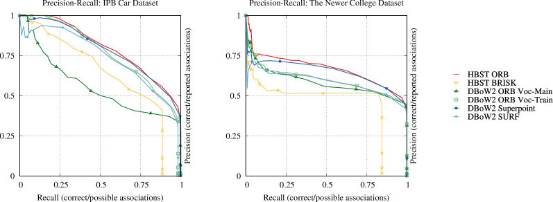
Figure 5: Precision-Recall curves of the closures computed both with different combinations of feature extractors - image matchers on the LiDAR  intensity image. Greater accuracy is reported in general by ORB-HBST, ORB-DBOW2 and Superpoint-DBOW2.

Figure 6: Localization timings of different combinations of feature extractors - image matchers. As expected binary descriptors take lower time to extract and match compared to floating points one.

V Experimental Evaluation

This evaluation analyzes our implemented combination of feature extractors and VPR pipelines on intensity images generated from LiDAR scanner point clouds and intensity data. In more detail, we evaluate the following combinations:

• FAST - ORB - HBST

• FAST - BRISK - HBST

• FAST - ORB - DBoW2

• Superpoint - DBoW2

• FAST - SURF - DBoW2

We test these configurations on four datasets, three publicly available, and one self-recorded dataset using an automated car, see Tab. II for dataset details. All datasets provide some cue of the robot position independent from the LiDAR sensor, which we use to construct ground truth place information. This is usually done with an RTK-GPS or an external reference system. The ground truth is a set of matching pairs of scans acquired at nearby locations. A pair is a match if the scans’ recording locations are close according to the external system, and an ICP registration succeeds. We processed the datasets sequentially by adding the query image $\mathcal{I}_{q}$ to the database at each step. We obtain a set (potentially empty) of images similar to $\mathcal{I}_{q}$ at each query, and we verify these matches against the ground truth. From the returned images, we disregard those added within the most recent 120 steps. We do this to not positively bias the evaluation.

For each dataset, we tested the combination of feature extractor and image retrieval systems mentioned before. To quantify the performances of one run, we evaluated common statistical quantities - i.e., Precision and Recall. To this end, we introduce the terms true positive to indicate a loop-closure that is present in the ground truth database and false positive to indicate a wrong loop-closure. Analogously, a false negative represents a loop-closure that is present in the ground truth database but has not been reported by the method in analysis; a true negative represents its contrary. Hence, we can define Precision and Recall using the number of true positives $T_{p}$, false positives $F_{p}$, true negatives $T_{n}$ and false negatives $F_{n}$ as follows:

$$P=\frac{T_{p}}{T_{p}+F_{p}}\qquad R=\frac{T_{p}}{T_{p}+F_{n}}.$$ (4)

We use FAST as the keypoint detector apart from Superpoint that outputs pairs of keypoints and descriptors directly for all experiments. For each dataset, we extracted the following descriptors: ORB, BRISK as binary and Superpoint and SURF as floating point. As retrieval methods, we use HBST with parameters $\delta_{\mathrm{max}}=0.1$ and $N_{\mathrm{max}}=50$ for the binary features. We use DBoW2 for all features but BRISK, which is not supported in by default package, and we extend it to operate with Superpoint. Configuration of each feature extractor reflects Tab. I.

Since BoW approaches require a dictionary that depends on the sensor characteristics, we train such dictionaries using a portion of the datasets not used for the evaluation. In the plots, these curves are labeled with Voc-Train. More in detail, we train the vocabulary by using 3000 intensity images, a branching factor of 10, and a depth level of 5, using the classic euclidean distance to measure descriptor similarity over floating points and the Hamming distance for the binary ones. For comparison, we also report the results obtained with the image-based dictionaries packaged in the software release of DBoW2 (Voc-Main).

We conduct several experiments, varying the type of descriptor and VPR matcher. We report the precision-recall curves (Fig. 6), maximum harmonic mean (Tab. III, Fig. 4), localization timings (Fig. 6) and valid loop closures drawn on the trajectories (Fig. 4) of the most significant experiments.

Overall, existing VPR approaches shows usable results at negligible computation over the two most recent datasets (IPB Car and The Newer College [31]) (Fig. 6 - Fig. 6). Results obtained in KITTI [15] and Ford Campus [28] are not comparable with the other two modern datasets. The vertical resolution and the intensity quality were to low in KITTI and Ford Campus to detect stable features, and we were not able to produce acceptable results (Tab. III).

The Newer College [31]	IPB Car	Ford Campus [28]	KITTI [15]
0.6751	0.7088	0.115	0.097

TABLE III: Max $F_{1}$ score reached in full validation over the four datasets with combination of HBST [34] and ORB [33].

We obtain the best results by combining ORB with HBST and DBoW2. The combination Superpoint-DBoW2 shows a comparable performance. However, floating point descriptor comes with a higher computational cost, see Fig. 6. The accuracy on The Newer College dataset [31] is inferior to the one obtained on our self-recorded dataset called IPB Car. This is due to the small changes on the roll axis since this data has been recorded walking in the campus, which, in turn, translates into a higher viewpoint variation within the same dataset.

For the experimental campaign, we used a PC running Ubuntu 20.04, equipped with an Intel i7-10750H CPU@2.60GHz and 16GB of RAM. We run neural network-based feature detection on an NVIDIA GeForce GTX 1650Ti.

VI Conclusion

In this work, we provide an analysis of the performance of visual place recognition techniques for loop closing, applied to the intensity information of a 3D LiDAR scanner. We evaluated gold standard visual place recognition approaches on four different datasets. Except for one outdated LiDAR, which does not provide stable intensity measurements, this transfer was proved to be successful. On modern sensors with a high vertical resolution, we obtained encouraging results. Despite not proposing a new approach in this work, we believe that existing LiDAR-based mapping systems can easily benefit from our findings. We furthermore expect that one can improve the performance further by designing or learning descriptors that are specifically optimized for intensity cues of LiDAR scanners.

References

- [1] R. Arandjelovicand, P. Gronat, A. Torii, T. Pajdla, and J. Sivic. Netvlad: Cnn architecture for weakly supervised place recognition. In Proc. of the IEEE Conf. on Computer Vision and Pattern Recognition (CVPR), pages 5297–5307, 2016.
- [2] H. Bay, A. Ess, T. Tuytelaars, and L. Van Gool. Speeded-up robust features (SURF). Journal of Computer Vision and Image Understanding (CVIU), 110(3):346–359, 2008.
- [3] H. Bay, T. Tuytelaars, and L. Van Gool. Surf: Speeded up robust features. In Proc. of the Europ. Conf. on Computer Vision (ECCV), pages 404–417. Springer, 2006.
- [4] J. Behley and C. Stachniss. Efficient surfel-based slam using 3d laser range data in urban environments. In Proc. of Robotics: Science and Systems (RSS), 2018.
- [5] G. Bradski and A. Kaehler. Opencv. Dr. Dobb’s journal of software tools, 3, 2000.
- [6] X. Chen, T. Läbe, A. Milioto, T. Röhling, O. Vysotska, A. Haag, J. Behley, and C. Stachniss. OverlapNet: Loop Closing for LiDAR-based SLAM. In Proc. of Robotics: Science and Systems (RSS), 2020.
- [7] K. P. Cop, P. VK Borges, and R. Dubé. Delight: An efficient descriptor for global localisation using lidar intensities. In Proc. of the IEEE Intl. Conf. on Robotics & Automation (ICRA), pages 3653–3660, 2018.
- [8] B. Della Corte, I. Bogoslavskyi, C. Stachniss, and G. Grisetti. A general framework for flexible multi-cue photometric point cloud registration. In Proc. of the IEEE Intl. Conf. on Robotics & Automation (ICRA), pages 1–8, 2018.
- [9] M. Cummins and P. Newman. Highly scalable appearance-only SLAM - FAB-MAP 2.0. In Proc. of Robotics: Science and Systems (RSS), 2009.
- [10] J. Deschaud. Imls-slam: scan-to-model matching based on 3d data. In Proc. of the IEEE Intl. Conf. on Robotics & Automation (ICRA), pages 2480–2485, 2018.
- [11] D. DeTone, T. Malisiewicz, and A. Rabinovich. Superpoint: Self-supervised interest point detection and description. In Proc. of the IEEE Conf. on Computer Vision and Pattern Recognition Workshops (CVPR), pages 224–236, 2018.
- [12] D. Droeschel and S. Behnke. Efficient continuous-time slam for 3d lidar-based online mapping. In 2018 IEEE International Conference on Robotics and Automation (ICRA), pages 5000–5007. IEEE, 2018.
- [13] R. Dubé, D. Dugas, E. Stumm, J. Nieto, R. Siegwart, and C. Cadena. Segmatch: Segment based place recognition in 3d point clouds. In Proc. of the IEEE Intl. Conf. on Robotics & Automation (ICRA), pages 5266–5272, 2017.
- [14] D. Gálvez-López and J. D. Tardos. Bags of binary words for fast place recognition in image sequences. IEEE Trans. on Robotics (TRO), 28(5):1188–1197, 2012.
- [15] A. Geiger, P. Lenz, C. Stiller, and R. Urtasun. Vision meets robotics: The kitti dataset. Intl. Journal of Robotics Research (IJRR), 32(11):1231–1237, 2013.
- [16] J. Guo, P. VK Borges, C. Park, and A. Gawel. Local descriptor for robust place recognition using lidar intensity. IEEE Robotics and Automation Letters (RA-L), 4(2):1470–1477, 2019.
- [17] D. F. Huber and M. Hebert. Automatic three-dimensional modeling from reality. PhD thesis, 2002.
- [18] A. E. Johnson. Spin-images: a representation for 3-d surface matching. 1997.
- [19] S. Leutenegger, M. Chli, and R. Y. Siegwart. Brisk: Binary robust invariant scalable keypoints. In Proc. of the IEEE Intl. Conf. on Computer Vision (ICCV), pages 2548–2555. IEEE, 2011.
- [20] C. Linegar, W. Churchill, and P. Newman. Work Smart, Not Hard: Recalling Relevant Experiences for Vast-Scale but Time-Constrained Localisation. In Proc. of the IEEE Intl. Conf. on Robotics & Automation (ICRA), 2015.
- [21] D. G. Lowe. Distinctive Image Features from Scale-Invariant Keypoints. Intl. Journal of Computer Vision (IJCV), 60(2):91–110, 2004.
- [22] S. Lowry, N. Sünderhauf, P. Newman, J. J. Leonard, D. Cox, P. Corke, and M. J. Milford. Visual place recognition: A survey. IEEE Trans. on Robotics (TRO), 32(1):1–19, 2015.
- [23] M. Magnusson, H. Andreasson, A. Nüchter, and A. J. Lilienthal. Automatic appearance-based loop detection from three-dimensional laser data using the normal distributions transform. Journal of Field Robotics (JFR), 26(11-12):892–914, 2009.
- [24] E. Mendes, P. Kochand, and S. Lacroix. Icp-based pose-graph slam. In 2016 IEEE International Symposium on Safety, Security, and Rescue Robotics (SSRR), pages 195–200. IEEE, 2016.
- [25] M. Milford. Vision-based place recognition: how low can you go? Intl. Journal of Robotics Research (IJRR), 32(7):766–789, 2013.
- [26] M. Milford and G.F. Wyeth. SeqSLAM: Visual route-based navigation for sunny summer days and stormy winter nights. In Proc. of the IEEE Intl. Conf. on Robotics & Automation (ICRA), 2012.
- [27] T. Naseer, W. Burgard, and C. Stachniss. Robust Visual Localization Across Seasons. IEEE Trans. on Robotics (TRO), 2018.
- [28] G. Pandey, J. R. McBride, and R. M. Eustice. Ford campus vision and lidar data set. Intl. Journal of Robotics Research (IJRR), 30(13):1543–1552, 2011.
- [29] C. R. Qi, H. Su, K. Mo, and L. J. Guibas. Pointnet: Deep learning on point sets for 3d classification and segmentation. In Proc. of the IEEE Conf. on Computer Vision and Pattern Recognition (CVPR), pages 652–660, 2017.
- [30] C. R. Qi, L. Yi, H. Su, and L. J. Guibas. Pointnet++: Deep hierarchical feature learning on point sets in a metric space. In Proc. of the Conf. on Neural Information Processing Systems (NIPS), pages 5099–5108, 2017.
- [31] M. Ramezani, Y. Wang, M. Camurri, D. Wisth, M. Mattamala, and M. Fallon. The newer college dataset: Handheld lidar, inertial and vision with ground truth. In Proc. of the IEEE/RSJ Intl. Conf. on Intelligent Robots and Systems (IROS), 2020.
- [32] T. Röhling, J. Mack, and D. Schulz. A fast histogram-based similarity measure for detecting loop closures in 3-d lidar data. In Proc. of the IEEE/RSJ Intl. Conf. on Intelligent Robots and Systems (IROS), pages 736–741, 2015.
- [33] E. Rublee, V. Rabaud, K. Konolige, and G. Bradski. Orb: An efficient alternative to sift or surf. In Proc. of the IEEE Intl. Conf. on Computer Vision (ICCV), pages 2564–2571. IEEE, 2011.
- [34] D. Schlegel and G. Grisetti. Hbst: A hamming distance embedding binary search tree for feature-based visual place recognition. IEEE Robotics and Automation Letters (RA-L), 3(4):3741–3748, 2018.
- [35] B. Steder, G. Grisetti, and W. Burgard. Robust place recognition for 3d range data based on point features. In Proc. of the IEEE Intl. Conf. on Robotics & Automation (ICRA), pages 1400–1405. IEEE, 2010.
- [36] B. Steder, G. Grisetti, M. Van Loock, and W. Burgard. Robust on-line model-based object detection from range images. In Proc. of the IEEE/RSJ Intl. Conf. on Intelligent Robots and Systems (IROS), pages 4739–4744. IEEE, 2009.
- [37] B. Steder, M. Ruhnke, S. Grzonka, and W. Burgard. Place recognition in 3d scans using a combination of bag of words and point feature based relative pose estimation. In Proc. of the IEEE/RSJ Intl. Conf. on Intelligent Robots and Systems (IROS), pages 1249–1255. IEEE, 2011.
- [38] B. Steder, R. B. Rusu, K. Konolige, and W. Burgard. Point feature extraction on 3d range scans taking into account object boundaries. In Proc. of the IEEE Intl. Conf. on Robotics & Automation (ICRA), pages 2601–2608. IEEE, 2011.
- [39] E. Stumm, C. Mei, S. Lacroix, and M. Chli. Location Graphs for Visual Place Recognition. In Proc. of the IEEE Intl. Conf. on Robotics & Automation (ICRA), 2015.
- [40] M. Angelina Uy and G. Hee Lee. Pointnetvlad: Deep point cloud based retrieval for large-scale place recognition. In Proc. of the IEEE Conf. on Computer Vision and Pattern Recognition (CVPR), pages 4470–4479, 2018.
- [41] C. Valgren and A.J. Lilienthal. SIFT, SURF & Seasons: Appearance-Based Long-Term Localization in Outdoor Environments. Journal on Robotics and Autonomous Systems (RAS), 85(2):149–156, 2010.
- [42] O. Vysotska and C. Stachniss. Lazy Data Association For Image Sequences Matching Under Substantial Appearance Changes. IEEE Robotics and Automation Letters (RA-L), 1(1):213–220, 2016.
- [43] O. Vysotska and C. Stachniss. Effective Visual Place Recognition Using Multi-Sequence Maps. IEEE Robotics and Automation Letters (RA-L), 4:1730–1736, 2019.
- [44] A. Zaganidis, M. Magnusson, T. Duckett, and G. Cielniak. Semantic-assisted 3d normal distributions transform for scan registration in environments with limited structure. In Proc. of the IEEE/RSJ Intl. Conf. on Intelligent Robots and Systems (IROS), pages 4064–4069. IEEE, 2017.
- [45] A. Zaganidis, A. Zerntev, T. Duckett, and G. Cielniak. Semantically assisted loop closure in slam using ndt histograms. In Proc. of the IEEE/RSJ Intl. Conf. on Intelligent Robots and Systems (IROS), pages 4562–4568, 2019.
- [46] J. Zhang and S. Singh. Loam: Lidar odometry and mapping in real-time. In Proc. of Robotics: Science and Systems (RSS), volume 2, 2014.
- [47] J. Zhang and S. Singh. Visual-lidar odometry and mapping: Low-drift, robust, and fast. In Proc. of the IEEE Intl. Conf. on Robotics & Automation (ICRA), pages 2174–2181, 2015.