DoubleML - An Object-Oriented Implementation of Double Machine Learning in R

Abstract

The R package DoubleML implements the double/debiased machine learning framework of Chernozhukov et al. (2018). It provides functionalities to estimate parameters in causal models based on machine learning methods. The double machine learning framework consist of three key ingredients: Neyman orthogonality, high-quality machine learning estimation and sample splitting. Estimation of nuisance components can be performed by various state-of-the-art machine learning methods that are available in the mlr3 ecosystem. DoubleML makes it possible to perform inference in a variety of causal models, including partially linear and interactive regression models and their extensions to instrumental variable estimation. The object-oriented implementation of DoubleML enables a high flexibility for the model specification and makes it easily extendable. This paper serves as an introduction to the double machine learning framework and the R package DoubleML. In reproducible code examples with simulated and real data sets, we demonstrate how DoubleML users can perform valid inference based on machine learning methods.

Keywords— Machine Learning, Causal Inference, Causal Machine Learning, R, mlr3, Object Orientation

1 Introduction

Structural equation models provide a quintessential framework for conducting causal inference in statistics, econometrics, machine learning (ML), and other data sciences. The package DoubleML for R (R Core Team, 2020) implements partially linear and interactive structural equation and treatment effect models with high-dimensional confounding variables as considered in Chernozhukov et al. (2018). Estimation and tuning of the machine learning models is based on the powerful functionalities provided by the mlr3 package and the mlr3 ecosystem (Lang et al., 2019). A key element of double machine learning (DML) models are score functions identifying the estimates for the target parameter. These functions play an essential role for valid inference with machine learning methods because they have to satisfy a property called Neyman orthogonality. With the score functions as key elements, DoubleML implements double machine learning in a very general way using object orientation based on the R6 package (Chang, 2020b). Currently, DoubleML implements the double / debiased machine learning framework as established in Chernozhukov et al. (2018) for

• partially linear regression models (PLR),

• partially linear instrumental variable regression models (PLIV),

• interactive regression models (IRM), and

• interactive instrumental variable regression models (IIVM).

The object-oriented implementation of DoubleML is very flexible. The model classes DoubleMLPLR, DoubleMLPLIV, DoubleMLIRM and DoubleIIVM implement the estimation of the nuisance functions via machine learning methods and the computation of the Neyman-orthogonal score function. All other functionalities are implemented in the abstract base class DoubleML, including estimation of causal parameters, standard errors, $t$-tests, confidence intervals, as well as valid simultaneous inference through adjustments of $p$-values and estimation of joint confidence regions based on a multiplier bootstrap procedure. In combination with the estimation and tuning functionalities of mlr3 and its ecosystem, this object-oriented implementation enables a high flexibility for the model specification in terms of

• the machine learning methods for estimation of the nuisance functions,

• the resampling schemes,

• the double machine learning algorithm, and

• the Neyman-orthogonal score functions.

It further can be readily extended regarding

• new model classes that come with Neyman-orthogonal score functions being linear in the target parameter,

• alternative score functions via callables, and

• customized resampling schemes.

For example, it would be straightforward to extend DoubleML to mediation analysis (Farbmacher et al., 2022), sample selection models (Bia et al., 2020) or difference-in-differences (Chang, 2020a). As we will point out later, a key requirement for new model classes is a Neyman-orthogonal score.

Several other packages for estimation of causal effects based on machine learning methods exist for R. Probably the most popular packages are the grf package (Tibshirani et al., 2020), which implements generalized random forests (Athey et al., 2019), the package hdm (Chernozhukov et al., 2016) for inference based on the lasso estimator and the hdi package (Dezeure et al., 2015) for inference in high-dimensional models. Previous implementations of the double machine learning (DML) framework of Chernozhukov et al. (2018) have been provided by the package dmlmt (Knaus, 2021) with a focus on lasso estimation and causalDML (Knaus, 2020) for estimation of treatment effects under unconfoundedness. A variety of causal estimation methods, including treatment effect estimators that are based on double machine learning and causal mediation analysis, is implemented in causalweight (Bodory and Huber, 2020). The R package AIPW (Zhong and Naimi, 2021) implements estimation of average treatment effects of a binary treatment variable by augmented inverse probability weighting based on machine learning algorithms and integrates well with the tlverse ecosystem discussed later.

In Python, EconML (Microsoft Research, 2019) offers an implementation of the double machine learning framework for heterogeneous effects. We would like to mention that the R package DoubleML was developed together with a Python twin (Bach et al., 2021) that is based on scikit-learn (Pedregosa et al., 2011). The Python package is also available via GitHub, the Python Package Index (PyPI), and conda-forge. Moreover, Kurz (2021) provides a serverless implementation of the Python module DoubleML.

An alternative approach, which was developed before the double machine learning framework, is the so-called Targeted Learning framework, and its software implementations and ecosystem (tlverse). For an overview and introduction to this approach and its implementations, we refer to the extensive tlverse handbook (van der Laan et al., 2022). Relevant R packages include SuperLearner (Polley et al., 2021) for flexible estimation using machine learning and tmle (Gruber and van der Laan, 2012) which implements estimation of causal parameters using targeted maximum likelihood estimation (TMLE). sl3 (Coyle et al., 2021) and tmle3 (Coyle, 2021) are recent extensions of the tlverse for object-oriented implementation of machine learning algorithms and a unified interface for TMLE.

The rest of the paper is structured as follows: In Section 2, we briefly demonstrate how to install the DoubleML package and give a short motivating example to illustrate the major idea behind the double machine learning approach. Section 3 introduces the main causal model classes implemented in DoubleML. Section 4 shortly summarizes the main ideas behind the double machine learning approach and reviews the key ingredients required for valid inference based on machine learning methods. Section 5 presents the main steps and algorithms of the double machine learning procedure for inference on one or multiple target parameters. Section 6 provides more detailed insights on the implemented classes and methods of DoubleML. Section 7 contains real-data and simulation examples for estimation of causal parameters using the DoubleML package. Additionally, this section provides a brief simulation study that illustrates the validity of the implemented methods in finite samples. Section 8 concludes the paper. The code output that has been suppressed in the main text and further information regarding the simulations are presented in the Appendix. To make the code examples fully reproducible, the entire code is available at https://github.com/DoubleML/DoubleMLReplicationCode.

2 Getting Started

2.1 Installation

The latest CRAN release of DoubleML can be installed using the command

install.packages("DoubleML")

Alternatively, the development version can be downloaded and installed from the GitHub repository using the command (previous installation of the remotes package is required)

remotes::install_github("DoubleML/doubleml-for-r")

Among others, DoubleML depends on the R package R6 for object oriented implementation, data.table (Dowle and Srinivasan, 2020) for the underlying data structure, as well as the packages mlr3 (Lang et al., 2019), mlr3learners (Lang et al., 2020a) and mlr3tuning (Becker et al., 2020) for estimation of machine learning methods, model tuning and parameter handling. Moreover, the underlying packages of the machine learning methods that are called in mlr3 or mlr3learners must be installed, for example the packages glmnet for lasso estimation (Friedman et al., 2010) or ranger (Wright and Ziegler, 2017) for random forests.

Load the package after completed installation.

library(DoubleML)

2.2 A Motivating Example: Basics of Double Machine Learning

In the following, we provide a brief summary of and motivation to double machine learning methods and show how the corresponding methods provided by the DoubleML package can be applied. The data generating process (DGP) is based on the introductory example in Chernozhukov et al. (2018). We consider a partially linear model: Our major interest is to estimate the causal parameter $\theta$ in the following regression equation

$$\begin{aligned} y_{i}=\theta d_{i}+g_{0}(x_{i})+\zeta_{i},&&\zeta_{i}\sim\mathcal{N}(0,1),\end{aligned}$$

with covariates $x_{i}\sim\mathcal{N}(0,\Sigma)$, where $\Sigma$ is a matrix with entries $\Sigma_{kj}=0.7^{|j-k|}$. In the following, the regression relationship between the treatment variable $d_{i}$ and the covariates $x_{i}$ will play an important role

$$\begin{aligned} d_{i}=m_{0}(x_{i})+v_{i},&&v_{i}\sim\mathcal{N}(0,1).\\ \end{aligned}$$

The nuisance functions $m_{0}$ and $g_{0}$ are given by

$$m_{0}(x_{i}) =x_{i,1}+\frac{1}{4}\frac{\exp(x_{i,3})}{1+\exp(x_{i,3})},$$

$$g_{0}(x_{i}) =\frac{\exp(x_{i,1})}{1+\exp(x_{i,1})}+\frac{1}{4}x_{i,3}.$$

We construct a setting with $n=500$ observations and $p=20$ explanatory variables to demonstrate the use of the estimators provided in DoubleML. Moreover, we set the true value of the parameter $\theta$ to $\theta=0.5$. The corresponding data generating process is implemented in the function make_plr_CCDHNR2018(). We start by generating a realization of a data set as a data.table object, which is subsequently used to create an instance of the data-backend of class DoubleMLData.

library(DoubleML)

alpha = 0.5

n_obs = 500

n_vars = 20

set.seed(1234)

data_plr = make_plr_CCDDHNR2018(alpha = alpha, n_obs = n_obs, dim_x = n_vars,

                                return_type = "data.table")

The data-backend implements the causal model: We specify that we perform inference on the effect of the treatment variable $d_{i}$ on the dependent variable $y_{i}$.

obj_dml_data = DoubleMLData$new(data_plr, y_col = "y", d_cols = "d")

In the next step, we choose the machine learning method as an object of class Learner from mlr3, mlr3learners (Lang et al., 2020a) or mlr3extralearners (Sonabend and Schratz, 2020). As we will point out later, we have to estimate two nuisance functions in order to perform valid inference in the partially linear regression model. Hence, we have to specify two learners. Moreover, we split the sample into two folds used for cross-fitting.

# Load mlr3 and mlr3learners package and suppress output during estimation

library(mlr3)

library(mlr3learners)

lgr::get_logger("mlr3")$set_threshold("warn")

# Initialize a random forests learner with specified parameters

ml_l = lrn("regr.ranger", num.trees = 100, mtry = n_vars, min.node.size = 2,

           max.depth = 5)

ml_m = lrn("regr.ranger", num.trees = 100, mtry = n_vars, min.node.size = 2,

           max.depth = 5)

ml_g = lrn("regr.ranger", num.trees = 100, mtry = n_vars, min.node.size = 2,

           max.depth = 5)

doubleml_plr = DoubleMLPLR$new(obj_dml_data,

                               ml_l, ml_m, ml_g,

                               n_folds = 2,

                               score = "IV-type")

To estimate the causal effect of variable $d_{i}$ on $y_{i}$, we call the fit() method.

doubleml_plr$fit()

doubleml_plr$summary()

## Estimates and significance testing of the effect of target variables
##   Estimate. Std. Error t value Pr(>|t|)
## d   0.51457    0.04522   11.38   <2e-16 ***
## ---
## Signif. codes:  0 ’***’ 0.001 ’**’ 0.01 ’*’ 0.05 ’.’ 0.1 ’ ’ 1

The output shows that the estimated coefficient is close to the true parameter $\theta=0.5$. Moreover, there is evidence to reject the null hypotheses $H_{0}:\theta=0$ at all common significance levels.

3 Key Causal Models

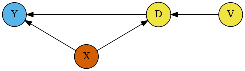
Figure 1: Causal diagram for PLR and IRM.

A causal diagram underlying Equation (1)-(2) and (5)-(6) under conditional exogeneity. Note that the causal link between $D$ and $Y$ is one-directional. Identification of the causal effect is confounded by $X$, and identification is achieved via $V$, which captures variation in $D$ that is independent of $X$. Methods to estimate the causal effect of $D$ must therefore approximately remove the effect of high-dimensional $X$ on $Y$ and $D$.

DoubleML provides estimation of causal effects in four different models: Partially linear regression models (PLR), partially linear instrumental variable regression models (PLIV), interactive regression models (IRM) and interactive instrumental variable regression models (IIVM). We will shortly introduce these models.

3.1 Partially Linear Regression Model (PLR)

Partially linear regression models (PLR), which encompass the standard linear regression model, play an important role in data analysis (Robinson, 1988). Partially linear regression models take the form

$$Y=D\theta_{0}+g_{0}(X)+\zeta,\quad \mathbb{E}(\zeta|D,X)=0,$$ (1)

$$D=m_{0}(X)+V,\quad \mathbb{E}(V|X)=0,$$ (2)

where $Y$ is the outcome variable and $D$ is the policy variable of interest. The high-dimensional vector $X=(X_{1},…,X_{p})$ consists of other confounding covariates, and $\zeta$ and $V$ are stochastic errors. Equation (1) is the equation of interest, and $\theta_{0}$ is the main regression coefficient that we would like to infer. If $D$ is conditionally exogenous (randomly assigned conditional on $X$), $\theta_{0}$ has the interpretation of a structural or causal parameter. The causal diagram supporting such interpretation is shown in Figure 1. The second equation keeps track of confounding, namely the dependence of $D$ on covariates/controls. The characteristics $X$ affect the policy variable $D$ via the function $m_{0}(X)$ and the outcome variable via the function $g_{0}(X)$. The partially linear model generalizes both linear regression models, where functions $g_{0}$ and $m_{0}$ are linear with respect to a collection of basis functions with respect to $X$, and approximately linear models.

An applied example from the economics literature is the analysis of the causal effect of 401(k) pension plans on employees’ net financial assets by Poterba et al. (1994) and Poterba et al. (1995). In these studies, which are based on observational data, it is argued that eligibility for 401(k) pension plans can be assumed to be conditionally exogenous, once it is controlled for a set of confounders $X$, for example income. Following this argumentation and modelling approach, the estimate on $\theta_{0}$ as obtained by a PLR can be interpreted as the average treatment effect of 401(k) eligibility on net financial assets. A reassessment and summary of the 401(k) example is available in Chernozhukov et al. (2018) as well as on the DoubleML website.

3.2 Partially Linear Instrumental Variable Regression Model (PLIV)

We next consider the partially linear instrumental variable regression model:

$$Y-D\theta_{0}=g_{0}(X)+\zeta,\quad \mathbb{E}(\zeta|Z,X)=0,$$ (3)

$$Z=m_{0}(X)+V,\quad \mathbb{E}(V|X)=0.$$ (4)

Note that this model is not a regression model unless $Z=D$. Model (3)-(4) is a canonical model in causal inference, going back to Wright (1928), with the modern difference being that $g_{0}$ and $m_{0}$ are nonlinear, potentially complicated functions of high-dimensional $X$. The idea of this model is that there is a structural or causal relation between $Y$ and $D$, captured by $\theta_{0}$, and $g_{0}(X)+\zeta$ is the stochastic error, partly explained by covariates $X$. $V$ and $\zeta$ are stochastic errors that are not explained by $X$. Since $Y$ and $D$ are jointly determined, we need an external factor, commonly referred to as an instrument, $Z$, to create exogenous variation in $D$. Note that $Z$ should affect $D$. The $X$ here serve again as confounding factors, so we can think of variation in $Z$ as being exogenous only conditional on $X$.

A simple contextual example is from biostatistics (Permutt and Hebel, 1989), where $Y$ is a health outcome and $D$ is an indicator of smoking. Thus, $\theta_{0}$ captures the effect of smoking on health. Health outcome $Y$ and smoking behavior $D$ are treated as being jointly determined. $X$ represents patient characteristics, and $Z$ could be a doctor’s advice not to smoke (or another behavioral treatment) that may affect the outcome $Y$ only through shifting the behavior $D$, conditional on characteristics $X$.

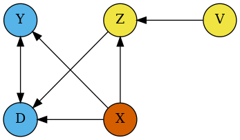
Figure 2: Causal diagram for PLIV and IIVM.

A causal diagram underlying Equation (3)-(4) and (7)-(8) under conditional exogeneity of $Z$. Note that the causal link between $D$ and $Y$ is bi-directional, so an instrument $Z$ is needed for identification. Identification is achieved via $V$ that captures variation in $Z$ that is independent of $X$. Equations (3) and (4) do not model the dependence between $D$ and $X$ and $Z$, though a necessary condition for identification is that $Z$ and $D$ are related after conditioning on $X$. Methods to estimate the causal effect of $D$ must approximately remove the effect of high-dimensional $X$ on $Y$, $D$, and $Z$. Removing the confounding effect of $X$ is done implicitly by the proposed procedure.

3.3 Interactive Regression Model (IRM)

We consider estimation of average treatment effects when treatment effects are fully heterogeneous, i.e. the response curves under control and treatment can be different nonparametric functions, and the treatment variable is binary, $D\in\{0,1\}$. We consider vectors $(Y,D,X)$ such that

$$Y=g_{0}(D,X)+U,\quad \mathbb{E}(U|X,D)=0,$$ (5)

$$D=m_{0}(X)+V,\quad \mathbb{E}(V|X)=0.$$ (6)

Since $D$ is not additively separable, this model is more general than the partially linear model for the case of binary $D$. A common target parameter of interest in this model is the average treatment effect (ATE),

$$\theta_{0}=\mathbb{E}[g_{0}(1,X)-g_{0}(0,X)].$$

Another common target parameter is the average treatment effect for the treated (ATTE),

$$\theta_{0}=\mathbb{E}[g_{0}(1,X)-g_{0}(0,X)|D=1].$$

In business applications, the ATTE is often the main interest, as it captures the treatment effect for those who have been affected by the treatment. A difference of the ATTE from the ATE might arise if the characteristics of the treated individuals differ from those of the general population.

The confounding factors $X$ affect the policy variable via the propensity score $m_{0}(X)$ and the outcome variable via the function $g_{0}(X)$. Both of these functions are unknown and potentially complex, and we can employ ML methods to learn them.

Taking up the 401(k) example from Section 3.1, the general idea for identification of $\theta_{0}$ using the IRM is similar. Once, we are able to account for all confounding variables $X$ in our analysis, we can consistently estimate the causal parameter $\theta_{0}$. A difference to the PLR refers to assumptions on the functional form of the main regression equation in 1 and 5, respectively. Whereas it is assumed that the effect of $D$ on $Y$ in the PLR model is additively separable, the IRM model comes with less restrictive assumptions. For example, it is possible that treatment effects are heterogeneous, i.e., vary across the population.

3.4 Interactive Instrumental Variable Model (IIVM)

We consider estimation of the local average treatment effect (LATE) with a binary treatment variable $D\in\{0,1\}$, and a binary instrument, $Z\in\{0,1\}$. As before, $Y$ denotes the outcome variable, and $X$ is the vector of covariates. In a setting where unobserved factors drive the take-up of the treatment $D$, the average treatment effect is no longer identified. However, if a valid instrumental variable is available that changes individuals’ decision to take up the treatment, it is possible to identify the LATE. The LATE measures the average causal effect for the subgroup of compliers, i.e., those individuals who receive the treatment only if the instrument takes value $Z=1$. Hence, the LATE is of interest in many studies, where the treatment assignment cannot be assumed to be conditionally independent. For a more detailed treatment of the LATE and the key assumptions required for its identification, we would like to refer to Imbens and Angrist (1994), Cunningham (2021) and Angrist and Pischke (2009).

The structural equation for the IIVM is:

$$Y=\ell_{0}(D,X)+\zeta,\quad \mathbb{E}(\zeta|Z,X)=0,$$ (7)

$$Z=m_{0}(X)+V,\quad \mathbb{E}(V|X)=0.$$ (8)

Consider the functions $g_{0}$, $r_{0}$, and $m_{0}$, where $g_{0}$ maps the support of $(Z,X)$ to $\mathbb{R}$ and $r_{0}$ and $m_{0}$ map the support of $(Z,X)$ and $X$ to $(\epsilon,1-\epsilon)$ for some $\epsilon\in(0,1/2)$, such that

$$Y=g_{0}(Z,X)+\nu,\quad \mathbb{E}(\nu|Z,X)=0,$$ (9)

$$D=r_{0}(Z,X)+U,\quad \mathbb{E}(U|Z,X)=0,$$ (10)

$$Z=m_{0}(X)+V,\quad \mathbb{E}(V|X)=0.$$ (11)

We are interested in estimating

$$\theta_{0} =\frac{\mathbb{E}[g_{0}(1,X)]-\mathbb{E}[g_{0}(0,X)]}{\mathbb{E}[r_{0}(1,X)]-\mathbb{E}[r_{0}(0,X)]}.$$

Under the well-known assumptions of Imbens and Angrist (1994), $\theta_{0}$ is the LATE – the average causal effect for compliers, in other words, those observations that would have $D=1$ if $Z$ were $1$ and would have $D=0$ if $Z$ were $0$.

In the smoking example from Section 3.2, the setting is similar to the section before, but now the binary treatment variable (“smoking”) is endogenous and is instrumented by a binary instrument variable $Z$ (“doctor’s advice”). In this example, the group of compliers would comprise those individuals who quit smoking once their doctor advises them to do so and would otherwise continue to smoke. Similar to the comparison of the IRM model and the PLR model, the IIVM model does not impose the assumptions of linearity and additive separability that are maintained in the PLIV.

4 Basic Idea and Key Ingredients of Double Machine Learning

4.1 Basic Idea behind Double Machine Learning for the PLR Model

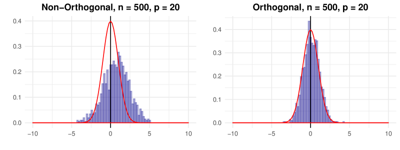
Figure 3: Performance of non-orthogonal and orthogonal estimators in a simulated data example.

Left panel: Histogram of the studentized naive estimator $\hat{\theta}^{naive}_{0}$. $\hat{\theta}^{naive}_{0}$ is based on estimation of $g_{0}$ and $m_{0}$ with random forests and a non-orthogonal score function. Data sets are simulated according to the data generating process in Section 2.2. Data generation and estimation are repeated 1000 times. Right panel: Histogram of the studentized DML estimator $\tilde{\theta}_{0}$. $\tilde{\theta}_{0}$ is based on estimation of $g_{0}$ and $m_{0}$ with random forests and an orthogonal score function provided in Equation (17). Note that the simulated data sets and parameters of the random forest learners are identical to those underlying the left panel.

Here we provide an intuitive discussion of how double machine learning works in the first model, the partially linear regression model. Naive application of machine learning methods directly to equations (1)-(2) may have a very high bias. Indeed, it can be shown that small biases in estimation of $g_{0}$, which are unavoidable in high-dimensional estimation, create a bias in the naive estimate of the main effect, $\hat{\theta_{0}}^{naive}$, which is sufficiently large to cause failure of conventional inference. The left panel in Figure 3 illustrates this phenomenon. The histogram presents the empirical distribution of the studentized estimator, $\hat{\theta}^{naive}_{0}$, as obtained in $1000$ independent repetitions of the data generating process presented in Section 2.2. The functions $g_{0}$ and $m_{0}$ in the PLR model are estimated with random forest learners and corresponding predictions are then plugged into a non-orthogonal score function. The regularization performed by the random forest learner leads to a bias in estimation of $g_{0}$ and $m_{0}$. Due to non-orthogonality of the score, this translates into a considerable bias of the main estimator $\hat{\theta_{0}}^{naive}$: The distribution of the studentized estimator $\hat{\theta}^{naive}_{0}$ is shifted to the right of the origin and differs substantially from a normal distribution that would be obtained if the regularization bias was negligible as shown by the red curve.

The PLR model above can be rewritten in the following residualized form:

$$W=V\theta_{0}+\zeta,\quad \mathbb{E}(\zeta|D,X)=0,$$ (12)

$$W=(Y-\ell_{0}(X)),\quad \ell_{0}(X)=\mathbb{E}[Y|X],$$ (13)

$$V=(D-m_{0}(X)),\quad m_{0}(X)=\mathbb{E}[D|X].$$ (14)

The variables $W$ and $V$ represent original variables after taking out or partialling out the effect of $X$. Note that $\theta_{0}$ is identified from this equation if $V$ has a non-zero variance.

Given identification, double machine learning for a PLR proceeds as follows

1. Estimate $\ell_{0}$ and $m_{0}$ by $\hat{\ell}_{0}$ and $\hat{m}_{0}$, which amounts to solving the two problems of predicting $Y$ and $D$ using $X$, using any generic ML method, giving us estimated residuals

   $$\hat{W}=Y-\hat{\ell}_{0}(X),$$

   and

   $$\hat{V}=D-\hat{m}_{0}(X).$$

   The residuals should be of a cross-validated form, as explained below in Algorithm 1 or 2, to avoid biases from overfitting.

2. Estimate $\theta_{0}$ by regressing the residual $\hat{W}$ on $\hat{V}$. Use the conventional inference for this regression estimator, ignoring the estimation error in the residuals.

The reason we work with this residualized form is that it eliminates the bias arising from solving the prediction problems in stage (1). The estimates $\hat{\ell}_{0}$ and $\hat{m}_{0}$ carry a regularization bias due to having to solve prediction problems well in high-dimensions. However, the nature of the estimating equation for $\theta_{0}$ are such that these biases are eliminated to the first order, as explained below. This results in a high-quality low-bias estimator $\tilde{\theta}_{0}$ of $\theta_{0}$, as illustrated in the right panel of Figure 3. The estimator is adaptive in the sense that the first stage estimation errors do not affect the second stage errors.

4.2 Key Ingredients of the Double Machine Learning Inference Approach

Our goal is to construct high-quality point and interval estimators for $\theta_{0}$ when $X$ is high-dimensional and we employ machine learning methods to estimate the nuisance functions such as $g_{0}$ and $m_{0}$. Example ML methods include lasso, random forests, boosted trees, deep neural networks, and ensembles or aggregated versions of these methods.

We shall use a method-of-moments estimator for $\theta_{0}$ based upon the empirical analog of the moment condition

$$\mathbb{E}[\psi(W;\theta_{0},\eta_{0})]=0,$$ (15)

where we call $\psi$ the score function, $W=(Y,D,X,Z)$, $\theta_{0}$ is the parameter of interest, and $\eta$ denotes nuisance functions with population value $\eta_{0}$.

The first key input of the inference procedure is using a score function $\psi(W;\theta;\eta)$ that satisfies (15), with $\theta_{0}$ being the unique solution, and that obeys the Neyman orthogonality condition

$$\partial_{\eta}\mathbb{E}[\psi(W;\theta_{0},\eta)]|_{\eta=\eta_{0}}=0.$$ (16)

Neyman orthogonality (16) ensures that the moment condition (15) used to identify and estimate $\theta_{0}$ is insensitive to small pertubations of the nuisance function $\eta$ around $\eta_{0}$. The derivative $\partial_{\eta}$ denotes the pathwise (Gateaux) derivative operator.

In general, it is important to distinguish whether machine learning methods are used for prediction or in the context of statistical inference. An accurate prediction rule for the nuisance parameters $\eta_{0}$ does not necessarily lead to a consistent estimator for the causal parameter $\theta_{0}$. Replacing the true value of $\eta_{0}$ by an ML estimator $\hat{\eta}_{0}$ likely introduces a bias, for example, due to heavy regularization in high-dimensional settings. If this bias is not taken into account, the estimator $\hat{\theta}_{0}$ will generally be inconsistent and not have an asymptotically normal distribution. Using a Neyman-orthogonal score makes estimation of the causal parameter $\theta_{0}$ robust against first order bias that arise from regularization. The Neyman orthogonality property is responsible for the adaptivity of the DML estimator – namely, the approximate distribution of $\hat{\theta}_{0}$ will not depend on the fact that the estimate $\hat{\eta}_{0}$ contains error, if the latter is mild. Other approaches, as targeted maximum likelihood and semiparametric sieves estimation recognize this as well. For a more detailed treatment of Neyman orthogonality we refer to Chernozhukov et al. (2018).

The right panel of Figure 3 presents the empirical distribution of the studentized DML estimator $\tilde{\theta}_{0}$ that is based on an orthogonal score. Note that estimation is performed on the identical simulated data sets and with the same machine learning method as for the naive learner, which is displayed in the left panel. The histogram of the studentized estimator $\tilde{\theta}_{0}$ illustrates the favorable performance of the double machine learning estimator, which is based on an orthogonal score: The DML estimator is robust to the bias that is generated by regularization. The estimator is approximately unbiased, is concentrated around $0$ and the distribution is well-approximated by the normal distribution.

• PLR score: In the PLR model, we can employ two alternative score functions. We will shortly indicate the option for initialization of a model object in DoubleML to clarify how each score can be implemented. Using the option score = "partialling out" leads to estimation of the score function

  $$\begin{aligned} &\psi(W;\theta,\eta):=\left(Y-\ell(X)-\theta(D-m(X))\right)\left(D-m(X)\right),\\ &\eta=(\ell,m),\quad\eta_{0}=(\ell_{0},m_{0}),\end{aligned}$$ (17)

  where $W=(Y,D,X)$ and $\ell$ and $m$ are $P$-square-integrable functions mapping the support of $X$ to $\mathbb{R}$, whose true values are given by

  $$\ell_{0}(X)=\mathbb{E}[Y|X],\quad m_{0}(X)=\mathbb{E}[D|X].$$

  Alternatively, it is possible to use the following score function for the PLR via the option score = "IV-type"

  $$\begin{aligned} &\psi(W;\theta,\eta):=\left(Y-D\theta-g(X)\right)\left(D-m(X)\right),&\eta=(g,m),\quad\eta_{0}=(g_{0},m_{0}),\end{aligned}$$ (18)

  with $g$ and $m$ being $P$-square-integrable functions mapping the support of $X$ to $\mathbb{R}$ with values given by

  $$g_{0}=\mathbb{E}[Y-D\theta_{0}|X],\quad m_{0}(X)=\mathbb{E}[D|X].$$

  The scores above are Neyman-orthogonal by elementary calculations. Now, it is possible to see the connections to the residualized system of equations presented in Section 4.1.

• PLIV score: In the PLIV model, we can employ two alternative score functions. Using the option score = "partialling out" leads to estimation of the score function

  $$\begin{aligned} &\psi(W;\theta,\eta):=\left(Y-\ell(x)-\theta(D-r(X))\right)\left(Z-m(X)\right),\\ &\eta=(\ell,m,r),\quad\eta_{0}=(\ell_{0},m_{0},r_{0}),\end{aligned}$$ (19)

  where $W=(Y,D,X,Z)$ and $\ell$, $m$, and $r$ are $P$-square integrable functions mapping the support of $X$ to $\mathbb{R}$, whose true values are given by

  $$\ell_{0}(X)=\mathbb{E}[Y|X],\quad r_{0}(X)=\mathbb{E}[D|X],\quad m_{0}(X)=\mathbb{E}[Z|X].$$

  Alternatively, it is possible to use the following score function for the PLIV via the option score = "IV-type"

  $$\begin{aligned} &\psi(W;\theta,\eta):=\left(Y-D\theta-g(X)\right)\left(Z-m(X)\right),&\eta=(g,m),\quad\eta_{0}=(g_{0},m_{0}),\end{aligned}$$ (20)

  with $g$ and $m$ being $P$-square-integrable functions mapping the support of $X$ to $\mathbb{R}$ with values given by

  $$g_{0}=\mathbb{E}[Y-D\theta_{0}|X],\quad m_{0}(X)=\mathbb{E}[Z|X].$$

• IRM score: For estimation of the ATE parameter of the IRM model, we employ the score (score = "ATE")

  $$\begin{aligned} &\psi(W;\theta,\eta):=\left(g(1,X)-g(0,X)\right)+\frac{D(Y-g(1,X))}{m(X)}-\frac{(1-D)(Y-g(0,X))}{1-m(X)}-\theta,\\ &\eta=(g,m),\quad\eta_{0}=(g_{0},m_{0}),\end{aligned}$$ (21)

  where $W=(Y,D,X)$ and $g$ and $m$ map the support of $(D,X)$ to $\mathbb{R}$ and the support of $X$ to $(\epsilon,1-\epsilon)$, respectively, for some $\epsilon\in(0,1/2)$, whose true values are given by

  $$g_{0}(D,X)=\mathbb{E}[Y|D,X],\quad m_{0}(x)=\mathbb{P}[D=1|X].$$

  This orthogonal score is based on the influence function for the mean for missing data from Robins and Rotnitzky (1995). For estimation of the ATTE parameter in the IRM, we use the score (score = "ATTE")

  $$\begin{aligned} &\psi(W;\theta,\eta):=\frac{D(Y-g(0,X))}{p}-\frac{m(X)(1-D)(Y-g(0,X))}{p(1-m(x))}-\frac{D}{p}\theta,\\ &\eta=(g,m,p),\quad\eta_{0}=(g_{0},m_{0},p_{0}),\end{aligned}$$ (22)

  where $p_{0}=\mathbb{P}(D=1)$. Note that this score does not require estimating $g_{0}(1,X)$.

• IIVM score: To estimate the LATE parameter in the IIVM, we will use the score (score = "LATE")

  $$\begin{aligned} \psi:=&g(1,X)-g(0,X)+\frac{Z(Y-g(1,X))}{m(X)}-\frac{(1-Z)(Y-g(0,X))}{1-m(X)}\\ &-\left(r(1,x)-r(0,X)+\frac{Z(D-r(1,x)}{m(X)}-\frac{(1-Z)(D-r(0,X)}{1-m(X)}\right)\times\theta,\\ &\eta=(g,m,r),\quad\eta_{0}=(g_{0},m_{0},r_{0}),\end{aligned}$$ (23)

  where $W=(Y,D,X,Z)$ and the nuisance parameter $\eta=(g,m,r)$ consists of $P$-square integrable functions $g$, $m$, and $r$, with $g$ mapping the support of $(Z,X)$ to $\mathbb{R}$ and $m$ and $r$, respectively, mapping the support of $(Z,X)$ and $X$ to $(\epsilon,1-\epsilon)$ for some $\epsilon\in(0,1/2)$.

The second key input is the use of high-quality machine learning estimators for the nuisance parameters.

For instance, in the PLR model, we need to have access to consistent estimators of $g_{0}$ and $m_{0}$ with respect to the $L^{2}(P)$ norm $\lVert\cdot\lVert_{P,2}$, such that

$$\lVert\hat{m}_{0}-m_{0}\lVert_{P,2}+\lVert\hat{\ell}_{0}-\ell_{0}\lVert_{P,2}\leq o(N^{-1/4}).$$ (24)

In the PLIV model, the sufficient condition is

$$\lVert\hat{r}_{0}-r_{0}\lVert_{P,2}+\lVert\hat{m}_{0}-m_{0}\lVert_{P,2}+\lVert\hat{\ell}_{0}-\ell_{0}\lVert_{P,2}\leq o(N^{-1/4}).$$ (25)

These conditions are plausible for many ML methods. Different structured assumptions on $\eta_{0}$ lead to the use of different machine-learning tools for estimating $\eta_{0}$ as listed in Chernozhukov et al. (2018, pp. 22-23):

1. The assumption of approximate or exact sparsity for $\eta_{0}$ with respect to some set of regressors, known as dictionary in computer science, calls for the use of sparsity-based machine learning methods, for example the lasso estimator, post-lasso, $l_{2}$-boosting, or forward selection, among others.

2. The assumption of density of $\eta_{0}$ with respect to some dictionary calls for density-based estimators such as the ridge. Mixed structures based on sparsity and density suggest the use of elastic net or lava.

3. If $\eta_{0}$ can be well approximated by tree-based methods, regression trees and random forests are suitable.

4. If $\eta_{0}$ can be well approximated by sparse, shallow or deep neural networks, $l_{1}$-penalized neural networks, shallow neural networks or deep neural networks are attractive.

For most of these ML methods, performance guarantees are available that make it possible to satisfy the theoretical requirements. For deep learning results can be found in Farrell et al. (2021), for lasso in Bühlmann and Van De Geer (2011). Moreover, if $\eta_{0}$ can be well approximated by at least one model mentioned in the list above, ensemble or aggregated methods (Wolpert, 1992; Breiman, 1996) can be used. Ensemble and aggregation methods ensure that the performance guarantee is approximately no worse than the performance of the best method (Van der Laan et al., 2007; Dudoit and van der Laan, 2005).

The third key input is to use a form of sample splitting at the stage of producing the estimator of the main parameter $\theta_{0}$, which allows to avoid biases arising from overfitting.

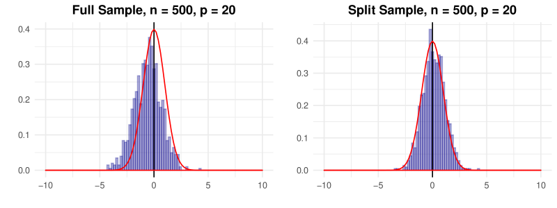
Figure 4: Performance of orthogonal estimators based on full sample and sample splitting in a simulated data example.

Left panel: Histogram of the studentized estimator $\hat{\theta}^{nosplit}_{0}$. $\hat{\theta}^{nosplit}_{0}$ is based on estimation of $g_{0}$ and $m_{0}$ with random forests and a procedure without sample-splitting: The entire data set is used for learning the nuisance terms and estimation of the orthogonal score. Data sets are simulated according to the data generating process in Section 2.2. Data generation and estimation are repeated 1000 times. Right panel: Histogram of the studentized DML estimator $\tilde{\theta}_{0}$. $\tilde{\theta}_{0}$ is based on estimation of $g_{0}$ and $m_{0}$ with random forests and the cross-fitting described in Algorithm 2. Note that the simulated data sets and parameters of the random forest learners are identical to those underlying the left panel.

Biases arising from overfitting could result from using highly complex fitting methods such as boosting, random forests, ensemble, and hybrid machine learning methods. We specifically use cross-fitted forms of the empirical moments, as detailed below in Algorithms 1 and 2, in estimation of $\theta_{0}$. If the same samples would be used to estimate $\eta_{0}$ and the causal parameter $\theta_{0}$, we may end up with very large bias, which we refer to as an overfitting bias. This is illustrated in Figure 4. The left panel shows the histogram of a studentized estimator $\hat{\theta}^{nosplit}_{0}$ with $\hat{\theta}^{nosplit}_{0}$ being obtained from solving the orthogonal score of Equation (17) without sample splitting. All observations are used to learn functions $g_{0}$ and $m_{0}$ in the PLR model and to solve the score $\frac{1}{N}\sum_{i}^{N}\psi(W_{i};\hat{\theta}^{nosplit}_{0},\hat{\eta}_{0})$. Consequently, this overfitting bias leads to a clearly visible shift of the empirical distribution to the left. The double machine learning estimator underlying the histogram in the right panel is obtained with cross-fitting according to Algorithm 2. The sample-splitting procedure makes it possible to completely eliminate the bias induced by overfitting.

5 The Double Machine Learning Inference Method

5.1 Double Machine Learning for Estimation of a Causal Parameter

We assume that we have a sample $(W_{i})^{N}_{i_{1}}$, modeled as i.i.d. copies of $W=(Y,D,Z,X)$, whose law is determined by the probability measure $P$. We assume that $N$ is divisible by $K$ in order to simplify the notation. Let $\mathbb{E}_{N}$ denote the empirical expectation

$$\mathbb{E}_{N}[g(W)]:=\frac{1}{N}\sum_{i=1}^{N}g(W_{i}).$$

Algorithm 1: DML1. (Generic double machine learning with cross-fitting)

1. Inputs: Choose a model (PLR, PLIV, IRM, IIVM), provide data $(W_{i})^{N}_{i=1}$, a Neyman-orthogonal score function $\psi(W;\theta,\eta)$, which depends on the model being estimated, and specify machine learning methods for $\eta$.

2. Train ML predictors on folds: Take a $K$-fold random partition $(I_{k})_{k=1}^{K}$ of observation indices $[N]=\{1,\ldots,N\}$ such that the size of each fold $I_{k}$ is $n=N/K$. For each $k\in[K]=\{1,\ldots,K\}$, construct a high-quality machine learning estimator

   $$\hat{\eta}_{0,k}=\hat{\eta}_{0,k}\big{(}(W_{i})_{i\not\in I_{k}}\big{)}$$

   of $\eta_{0}$, where $x\mapsto\hat{\eta}_{0,k}(x)$ depends only on the subset of data $(W_{i})_{i\not\in I_{k}}$.

3. For each $k\in[K]$, construct the estimator $\check{\theta}_{0,k}$ as the solution to the equation

   $$\frac{1}{n}\sum_{i\in I_{k}}\psi(W_{i};\check{\theta}_{0,k},\hat{\eta}_{0,k})=0.$$ (26)

   The estimate of the causal parameter is obtained via aggregation

   $$\tilde{\theta}_{0}=\frac{1}{K}\sum_{k=1}^{K}\check{\theta}_{0,k}.$$

4. Output: The estimate of the causal parameter $\tilde{\theta}_{0}$ as well as the values of the evaluated score function are returned.

Algorithm 2: DML2. (Generic double machine learning with cross-fitting)

1. Inputs: Choose a model (PLR, PLIV, IRM, IIVM), provide data $(W_{i})^{N}_{i=1}$, a Neyman-orthogonal score function $\psi(W;\theta,\eta)$, which depends on the model being estimated, and specify machine learning methods for $\eta$.

2. Train ML predictors on folds: Take a $K$-fold random partition $(I_{k})_{k=1}^{K}$ of observation indices $[N]=\{1,\ldots,N\}$ such that the size of each fold $I_{k}$ is $n=N/K$. For each $k\in[K]=\{1,\ldots,K\}$, construct a high-quality machine learning estimator

   $$\hat{\eta}_{0,k}=\hat{\eta}_{0,k}\big{(}(W_{i})_{i\not\in I_{k}}\big{)}$$

   of $\eta_{0}$, where $x\mapsto\hat{\eta}_{0,k}(x)$ depends only on the subset of data $(W_{i})_{i\not\in I_{k}}$.

3. Construct the estimator for the causal parameter $\tilde{\theta}_{0}$ as the solution to the equation

   $$\frac{1}{N}\sum_{k=1}^{K}\sum_{i\in I_{k}}\psi(W_{i};\tilde{\theta}_{0},\hat{\eta}_{0,k})=0.$$ (27)

4. Output: The estimate of the causal parameter $\tilde{\theta}_{0}$ as well as the values of the evaluated score function are returned.

Both Algorithm 1 and 2 use out-of-sample predictions generated by ML learners in order to solve an orthogonal moment condition and, hence, share the same steps (1) and (2). However, the algorithms differ in the way the nuisance predictions are plugged into the score function and in the subsequent solution for $\theta_{0}$. In Algorithm 1, the score is solved on each of the $K$ folds and the estimate $\tilde{\theta}_{0}$ is obtained by averaging the $K$ preliminary estimators, $\check{\theta}_{0,k}$ with $k=1,\ldots,K$. According to Algorithm 2, the out-of-sample predictions $\hat{\eta}_{0}$ are all plugged into one score function, which is then solved to obtain the estimate $\tilde{\theta}_{0}$.

Remark 1 (Linear scores) The score for the models PLR, PLIV, IRM and IIVM are linear in $\theta$, having the form

$$\psi(W;\theta,\eta)=\psi_{a}(W;\eta)\theta+\psi_{b}(W;\eta),$$

hence the estimator $\tilde{\theta}_{0,k}$ for DML2 ($\check{\theta}_{0,k}$ for DML1) takes the form

$$\tilde{\theta}_{0}=-\left(\mathbb{E}_{N}[\psi_{a}(W;\eta)]\right)^{-1}\mathbb{E}_{N}[\psi_{b}(W;\eta)].$$ (28)

The linear score function representations of the PLR, PLIV, IRM and IIVM are

• PLR with score = "partialling out"

  $$\begin{aligned} \psi_{a}(W;\eta)&=-(D-m(X))(D-m(X)),\\ \psi_{b}(W;\eta)&=(Y-\ell(X))(D-m(X)).\end{aligned}$$ (29)

  PLR with score = "IV-type"

  $$\begin{aligned} \psi_{a}(W;\eta)&=-D(D-m(X)),\\ \psi_{b}(W;\eta)&=(Y-g(X))(D-m(X)).\end{aligned}$$ (30)

• PLIV with score = "partialling out"

  $$\begin{aligned} \psi_{a}(W;\eta)&=-(D-r(X))(Z-m(X)),\\ \psi_{b}(W;\eta)&=(Y-\ell(X))(Z-m(X)).\end{aligned}$$ (31)

  PLIV with score = "IV-type"

  $$\begin{aligned} \psi_{a}(W;\eta)&=-D(Z-m(X)),\\ \psi_{b}(W;\eta)&=(Y-g(X))(Z-m(X)).\end{aligned}$$ (32)

• IRM with score = "ATE"

  $$\begin{aligned} \psi_{a}(W;\eta)&=-1,\\ \psi_{b}(W;\eta)&=g(1,X)-g(0,X)+\frac{D(Y-g(1,X))}{m(X)}-\frac{(1-D)(Y-g(0,X))}{1-m(x)}.\end{aligned}$$ (33)

  IRM with score = "ATTE"

  $$\begin{aligned} \psi_{a}(W;\theta,\eta)&=-\frac{D}{p}\\ \psi_{b}(W;\theta,\eta)&=\frac{D(Y-g(0,X))}{p}-\frac{m(X)(1-D)(Y-g(0,X))}{p(1-m(x))}\\ \end{aligned}$$ (34)

• IIVM with score = "LATE"

  $$\begin{aligned} \psi_{a}(W;\eta)&=-\bigg{(}r(1,X)-r(0,X)+\frac{Z(D-r(1,X))}{m(X)}-\frac{(1-Z)(D-r(0,X))}{1-m(x)}\bigg{)},\\ \psi_{b}(W;\eta)&=g(1,X)-g(0,X)+\frac{Z(Y-g(1,X))}{m(X)}-\frac{(1-Z)(Y-g(0,X))}{1-m(x)}.\end{aligned}$$ (35)

Remark 2 (Sample Splitting) In Step (2) of the Algorithm DML1 and DML2, the estimator $\hat{\eta}_{0,k}$ can generally be an ensemble or aggregation of several estimators as long as we only use the data $(W_{i})_{i\not\in I_{k}}$ outside the $k$-th fold to construct the estimators.

Remark 3 (Recommendation) We have found that $K=4$ or $K=5$ to work better than $K=2$ in a variety of empirical examples and in simulations. The default for the option n_folds that implements the value of $K$ is n_folds=5. Moreover, we generally recommend to repeat the estimation procedure multiple times and use the estimates and standard errors as aggregated over multiple repetitions as described in Chernozhukov et al. (2018, pp. 30-31). This aggregation will be automatically executed if the number of repetitions n_rep is set to a value larger than 1.

The properties of the estimator are as follows.

Theorem 1

There exist regularity conditions, such that the estimator $\tilde{\theta}_{0}$ concentrates in a $1/\sqrt{N}$-neighborhood of $\theta_{0}$ and the sampling error $\sqrt{N}(\tilde{\theta}_{0}-\theta_{0})$ is approximately normal

$$\sqrt{N}(\tilde{\theta}_{0}-\theta_{0})\leadsto N(0,\sigma^{2}),$$

with mean zero and variance given by

$$\begin{aligned} \sigma^{2}&=J_{0}^{-2}\mathbb{E}(\psi^{2}(W;\theta_{0},\eta_{0})),\\ J_{0}&=\mathbb{E}(\psi_{a}(W;\eta_{0})).\end{aligned}$$

Algorithm 3: Variance Estimation and Confidence Intervals.

1. Inputs: Use the inputs and outputs from Algorithm 1 (DML1) or Algorithm 2 (DML2).

2. Variance and confidence intervals: Estimate the asymptotic variance of $\tilde{\theta}_{0}$ by

   $$\begin{aligned} \hat{\sigma}^{2}&=\hat{J}_{0}^{-2}\frac{1}{N}\sum_{k=1}^{K}\sum_{i\in I_{k}}\big{[}\psi(W_{i};\tilde{\theta}_{0},\hat{\eta}_{0,k})\big{]}^{2},\\ \hat{J}_{0}&=\frac{1}{N}\sum_{k=1}^{K}\sum_{i\in I_{k}}\psi_{a}(W_{i};\hat{\eta}_{0,k})\end{aligned}$$

   and form an approximate $(1-\alpha)$ confidence interval, which is asymptotically valid, as

   $$[\tilde{\theta}_{0}\pm\Phi^{-1}(1-\alpha/2)\hat{\sigma}/\sqrt{N}].$$

3. Output: Output variance estimator and the confidence interval.

Theorem 2

Under the same regularity condition, this interval contains $\theta_{0}$ for approximately $(1-\alpha)\times 100$ percent of data realizations

$$\mathbb{P}\left(\theta_{0}\in\left[\tilde{\theta}_{0}\pm\Phi^{-1}(1-\alpha/2)\hat{\sigma}/\sqrt{N}\right]\right)\rightarrow(1-\alpha).$$

Remark 4 (Brief literature overview on double machine learning) The presented double machine learning method was developed in Chernozhukov et al. (2018). The idea of using property (16) to construct estimators and inference procedures that are robust to small mistakes in nuisance parameters can be traced back to Neyman (1959) and has been used explicitly or implicitly in the literature on debiased sparsity-based inference (Belloni et al., 2011, 2014b; Javanmard and Montanari, 2014; van de Geer et al., 2014; Zhang and Zhang, 2014; Chernozhukov et al., 2015b) as well as (implicitly) in the classical semi-parametric learning theory with low-dimensional $X$ (Bickel et al., 1993; Newey, 1994; Van der Vaart, 2000; Van der Laan and Rose, 2011). These references also explain that if we use scores $\psi$ that are not Neyman-orthogonal in high dimensional settings, then the resulting estimators of $\theta_{0}$ are not $1/\sqrt{N}$ consistent and are generally heavily biased.

Remark 5 (Literature on sample splitting). Sample splitting has been used in the traditional semiparametric estimation literature to establish good properties of semiparametric estimators under weak conditions (Klaassen, 1987; Schick, 1986; Van der Vaart, 2000; Zheng and Laan, 2011). In sparse learning problems with high-dimensional $X$, sample splitting was employed in Belloni et al. (2012). There and here, the use of sample splitting results in weak conditions on the estimators of nuisance parameters, translating into weak assumptions on sparsity in the case of sparsity-based learning.

Remark 6 (Debiased machine learning). The presented approach builds upon and generalizes the approach of Belloni et al. (2011), Zhang and Zhang (2014), Javanmard and Montanari (2014), Javanmard and Montanari (2014), Javanmard and Montanari (2018), Belloni et al. (2014c), Belloni et al. (2014a), Bühlmann and van de Geer (2015), which considered estimation of the special case (1)-(2) using lasso without cross-fitting. This generalization, by relying upon cross-fitting, opens up the use of a much broader collection of machine learning methods and, in the case the lasso is used to estimate the nuisance functions, allows relaxation of sparsity conditions. All of these approaches can be seen as “debiasing” the estimation of the main parameter by constructing, implicitly or explicitly, score functions that satisfy the exact or approximate Neyman orthogonality.

5.2 Methods for Simultaneous Inference

In addition to estimation of target causal parameters, standard errors, and confidence intervals, the package DoubleML provides methods to perform valid simultaneous inference based on a multiplier bootstrap procedure introduced in Chernozhukov et al. (2013) and Chernozhukov et al. (2014) and suggested in high-dimensional linear regression models in Belloni et al. (2014a). Accordingly, it is possible to (i) construct simultaneous confidence bands for a potentially large number of causal parameters and (ii) adjust $p$-values in a test of multiple hypotheses based on the inferential procedure introduced above.

We consider a causal PLR with $p_{1}$ causal parameters of interest $\theta_{0,1},\ldots,\theta_{0,p_{1}}$ associated with the treatment variables $D_{1},\ldots,D_{p_{1}}$. The parameter of interest $\theta_{0,j}$ with $j=1,\ldots,p_{1}$ solves a corresponding moment condition

$$\mathbb{E}\left[\psi_{j}(W;\theta_{0,j},\eta_{0,j})\right]=0,$$ (36)

as for example considered in Belloni et al. (2018). To perform inference in a setting with multiple target coefficients $\theta_{0,j}$, the double machine learning procedure implemented in DoubleML iterates over the target variables of interest. During estimation of the effect of treatment $D_{j}$ on $Y$ as measured by the coefficient $\theta_{0,j}$, the remaining treatment variables enter the nuisance terms by default, i.e., they are added to the set of control variables $X$.

Algorithm 4: Multiplier bootstrap.

1. Inputs: Use the inputs and outputs from Algorithm 1 (DML1) or Algorithm 2 (DML2) and Algorithm 3 (Variance estimation) resulting in estimates $\tilde{\theta}_{0,1},\ldots,\tilde{\theta}_{0,p_{1}}$, and standard errors $\hat{\sigma}_{1},\ldots\hat{\sigma}_{p_{1}}$.

2. Multiplier bootstrap: Generate random weights $\xi_{i}^{b}$ for each bootstrap repetition $b=1,\ldots,B$ according to a normal (Gaussian) bootstrap, wild bootstrap or exponential bootstrap. Based on the estimated standard errors given by $\hat{\sigma}_{j}$ and $\hat{J}_{0,j}=\mathbb{E}_{N}(\psi_{a,j}(W;\eta_{0,j}))$, we obtain bootstrapped versions of the coefficients $\tilde{\theta}^{*,b}_{j}$ and bootstrapped $t$-statistics $t^{*,b}_{j}$ for $j=1,\ldots,p_{1}$

   $$\begin{aligned} \theta^{*,b}_{j}&=\frac{1}{\sqrt{N}\hat{J}_{0,j}}\sum_{k=1}^{K}\sum_{i\in I_{k}}\xi_{i}^{b}\cdot\psi_{j}(W_{i};\tilde{\theta}_{0,j},\hat{\eta}_{0,j;k}),\\ t^{*,b}_{j}&=\frac{1}{\sqrt{N}\hat{J}_{0,j}\hat{\sigma}_{j}}\sum_{k=1}^{K}\sum_{i\in I_{k}}\xi_{i}^{b}\cdot\psi_{j}(W_{i};\tilde{\theta}_{0,j},\hat{\eta}_{0,j;k}).\end{aligned}$$

3. Output: Output bootstrapped coefficients and test statistics.

Remark 7 (Computational efficiency) The multiplier bootstrap procedure of Chernozhukov et al. (2013) and Chernozhukov et al. (2014) is computationally efficient because it does not require resampling and reestimation of the causal parameters. Instead, it is sufficient to introduce a random pertubation of the score $\psi$ and solve for $\theta_{0}$, accordingly.

To construct simultaneous $(1-\alpha)$-confidence bands, the multiplier bootstrap presented in Algorithm 4 can be used to obtain a constant $c_{1-\alpha}$ that will guarantee asymptotic $(1-\alpha$) coverage

$$\left[\tilde{\theta}_{0,j}\pm c_{1-\alpha}\cdot\hat{\sigma}_{j}/\sqrt{N}\right].$$ (37)

The constant $c_{1-\alpha}$ is obtained in two steps.

1. Calculate the maximum of the absolute values of the bootstrapped $t$-statistics, $t^{*,b}_{j}$ in every repetition $b$ with $b=1,\ldots,B$.

2. Use the $(1-\alpha)$-quantile of the $B$ maxima statistics from Step 1 as $c_{1-\alpha}$ and construct simultaneous confidence bands according to Equation (37).

Moreover, it is possible to derive an adjustment method for $p$-values obtained from a test of multiple hypotheses, including classical adjustments such as the Bonferroni correction as well as the Romano-Wolf stepdown procedure (Romano and Wolf, 2005a, b). The latter is implemented according to the algorithm for adjustment of $p$-values as provided in Romano and Wolf (2016) and adapted to high-dimensional linear regression based on the lasso in Bach et al. (2018).

6 Implementation Details

In this section, we briefly provide information on the implementation details such as the class structure, the data-backend and the use of machine learning methods. Section 7 provides a demonstration of DoubleML in real-data and simulation examples. More information on the implementation can be found in the DoubleML User Guide, that is available online. All class methods are documented in the documentation of the corresponding class, which can be browsed online or, for example, by using the commands help(DoubleML), help(DoubleMLPLR), or help(DoubleMLData) in R. For an introduction to R6 we refer to the introduction of the online book for mlr3.

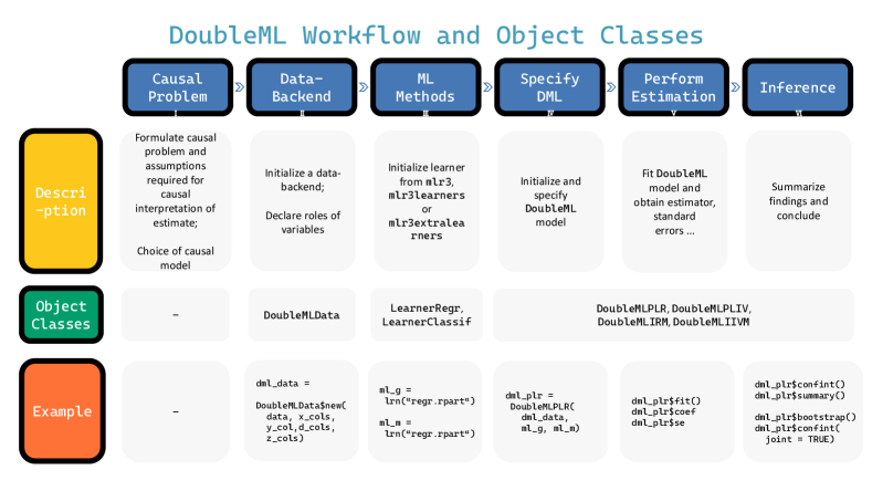
Figure 5: Flowchart with main steps and object classes in DoubleML.

The flowchart illustrates the basic steps for estimation of causal parameters with DoubleML. The diagram contains a short description of the main steps and lists the object classes used in each step. A short example demonstrates the use of the object classes and methods.

6.1 Class Structure

The implementation of DoubleML for R is based on object orientation as enabled by the the R6 package (Chang, 2020b). For an introduction to object orientation in R and the R6 package, we refer to the vignettes of the R6 package that are available online, Chapter 2.1 of Becker et al. (2021), and the chapters on object orientation in Wickham (2019). The structure of the classes are presented in Figure 6. Moreover, the flowchart in Figure 5 illustrates the main steps of an analysis in DoubleML and links them to the provided object classes. Figure 5 provides a short code demonstration, too. The abstract class DoubleML provides all methods for estimation and inference, for example the methods fit(), bootstrap(), confint(). All key components associated with estimation and inference are implemented in DoubleML, for example the sample splitting, the implementation of Algorithm 1 (DML1) and Algorithm 2 (DML2), the estimation of the causal parameters, and the computation of the scores $\psi(W;\theta,\eta)$. Only the model-specific properties and methods are allocated at the classes DoubleMLPLR (implementing the PLR), DoubleMLPLIV (PLIV), DoubleMLIRM (IRM), and DoubleMLIIVM (IIVM). For example, each of the models has one or several Neyman-orthogonal score functions that are implemented for the specific child classes.

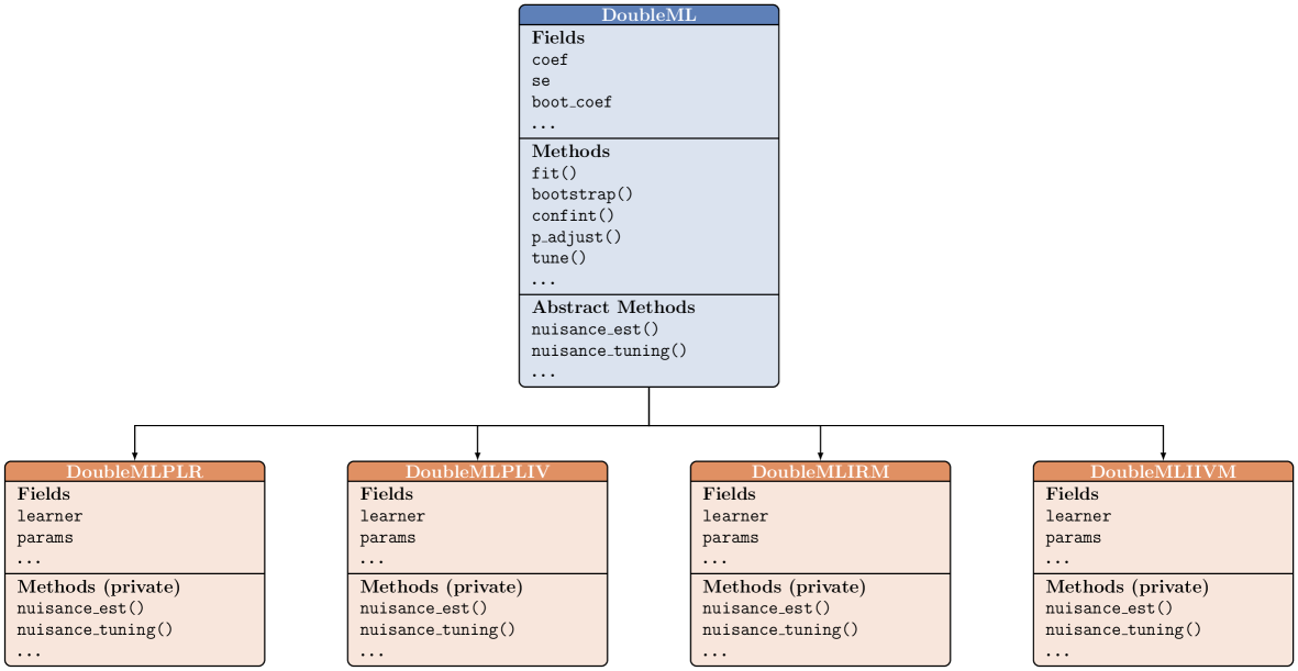
Figure 6: Class structure of the DoubleML package for R.

6.2 Data-Backend and Causal Model

The DoubleMLData class serves as the data-backend and implements the causal model of interest. The user is required to specify the roles of the variables in a data set at hand. Depending on the causal model considered, it is necessary to declare the dependent variable, the treatment variable(s), confounding variables(s), and, in the case of instrumental variable regression, one or multiple instruments. The data-backend can be initialized from a data.table (Dowle and Srinivasan, 2020). DoubleML provides wrappers to initialize from data.frame and matrix objects, as well.

6.3 Learners, Parameters and Tuning

Generally, all learners provided by the packages mlr3, mlr3learners and mlr3extralearners can be used for estimation of the nuisance functions of the structural models presented above. An interactive list of supported learners is available at the mlr3extralearners website. The mlr3extralearners package makes it possible to add new learners, as well. The performance of the double machine learning estimator $\tilde{\theta}_{0}$ will depend on the predictive quality of the used estimation method. Machine learning methods usually have several (hyper-)parameter that need to be adapted to a specific application. Tuning of model parameters can be either performed externally or internally. The latter is implemented in the method tune() and is further illustrated in an example in Section 7.6.2. Both cases build on the functionalities provided by the package mlr3tuning.

6.4 Modifications and Extensions

The flexible architecture of the DoubleML package allows users to modify the estimation procedure in many regards. Among others, users can provide customized sample splitting rules after initialization of the causal model via the method set_sample_splitting(). An example and the detailed requirements are provided in Section 7.7.1. Moreover, it is possible to adjust the Neyman-orthogonal score function by externally providing a customized function via the score option during initialization of the causal model object. A short example is presented in Section 7.7.2.

7 Estimation of Causal Parameters with DoubleML: Real-Data and Simulated Examples

In this section, we will first demonstrate the use of DoubleML in a real-data example, which is based on data from the Pennsylvania Reemployment Bonus experiment (Bilias, 2000). This empirical example has been used in Chernozhukov et al. (2018), as well. The goal in the empirical example is to estimate the causal parameter in a partially linear and an interactive regression model. We further provide a short example on how valid simultaneous inference can be performed with DoubleML. Finally, we present results from a short simulation study as a brief assessment of the finite-sample performance of the implemented estimators. Here we want to stress that in real world applications modelling choices of the estimation of the nuisance parameters and proper tuning of the parameters are very important. We would like to mention that the presented examples are mainly included for the purpose of illustration. In practice, we recommend to carefully choose and tune the ML learners in terms of their hyperparamaters.

7.1 Initialization of the Data-Backend

We begin our real-data example by downloading the Pennsylvania Reemployment Bonus data set. To do so, we use the call (a connection to the internet is required).

library(DoubleML)

# Load data as data.table

dt_bonus = fetch_bonus(return_type = "data.table")

# output suppressed for the sake of brevity

dt_bonus

The data-backend DoubleMLData can be initialized from a data.table object by specifying the dependent variable $Y$ via a character in y_col, the treatment variable(s) $D$ in d_cols, and the confounders $X$ via x_cols. Moreover, in IV models, an instrument can be specified via z_cols. In the next step, we assign the roles to the variables in the data set: y_col = 'inuidur1' serves as outcome variable $Y$, the column d_cols = 'tg' serves as treatment variable $D$ and the columns x_cols specify the confounders.

obj_dml_data_bonus = DoubleMLData$new(dt_bonus,

                                      y_col = "inuidur1",

                                      d_cols = "tg",

                                      x_cols = c("female", "black", "othrace",

                                                 "dep1", "dep2", "q2", "q3",

                                                 "q4", "q5", "q6", "agelt35",

                                                 "agegt54", "durable", "lusd",

                                                 "husd"))

# Print data backend: Lists main attributes and methods of a DoubleMLData object

obj_dml_data_bonus

## ================= DoubleMLData Object ==================
##
##
## ------------------ Data summary      ------------------
## Outcome variable: inuidur1
## Treatment variable(s): tg
## Covariates: female, black, othrace, dep1, dep2, q2, q3, q4, q5, q6, agelt35, agegt54, durable, lusd, husd
## Instrument(s):
## No. Observations: 5099

# Print data set (output suppressed)

obj_dml_data_bonus$data

Remark 8 (Interface for data.frame and matrix) To initialize an instance of the class DoubleMLData from a data.frame or a collection of matrix objects, DoubleML provides the convenient wrappers double_ml_data_from_data_frame() and double_ml_data_from_matrix(). Examples can be found in the user guide and in the corresponding documentation.

7.2 Initialization of the Causal Model

To initialize a PLR model, we have to provide a learner for each nuisance part in the model in Equation (1)-(2). In R, this is done by providing learners to the arguments ml_m for nuisance part $m$ and ml_l for nuisance part $\ell$. We can pass a learner as instantiated in mlr3 and mlr3learners, for example a random forest as provided by the R package ranger (Wright and Ziegler, 2017). Previous installation of ranger is required. Moreover, we can specify the score (allowed choices for PLR are "partialling out" or "IV-type") and the algorithm via the option dml_procedure (allowed choices "dml1" and "dml2") . Optionally, it is possible to change the number of folds used for sample splitting through n_folds and the number of repetitions via n_rep, if the sample splitting and estimation procedure should be repeated.

set.seed(31415) # required for reproducability of sample split

learner_l = lrn("regr.ranger", num.trees = 500,

                min.node.size = 2, max.depth = 5)

learner_m = lrn("regr.ranger", num.trees = 500,

                min.node.size = 2, max.depth = 5)

doubleml_bonus = DoubleMLPLR$new(obj_dml_data_bonus,

                                 ml_l = learner_l,

                                 ml_m = learner_m,

                                 score = "partialling out",

                                 dml_procedure = "dml1",

                                 n_folds = 5,

                                 n_rep = 1)

doubleml_bonus

## ================= DoubleMLPLR Object ==================
##
##
## ------------------ Data summary      ------------------
## Outcome variable: inuidur1
## Treatment variable(s): tg
## Covariates: female, black, othrace, dep1, dep2, q2, q3, q4, q5, q6, agelt35, agegt54,
##ΨΨdurable, lusd, husd
## Instrument(s):
## No. Observations: 5099
##
## ------------------ Score & algorithm ------------------
## Score function: partialling out
## DML algorithm: dml1
##
## ------------------ Machine learner   ------------------
## ml_l: regr.ranger
## ml_m: regr.ranger
##
## ------------------ Resampling        ------------------
## No. folds: 5
## No. repeated sample splits: 1
## Apply cross-fitting: TRUE
##
## ------------------ Fit summary       ------------------
##

7.3 Estimation of the Causal Parameter in a PLR Model

To perform estimation, call the fit() method. The output can be summarized using the method summary().

doubleml_bonus$fit()

doubleml_bonus$summary()

## Estimates and significance testing of the effect of target variables
##    Estimate. Std. Error t value Pr(>|t|)
## tg  -0.07438    0.03543  -2.099   0.0358 *
## ---
## Signif. codes:  0 ’***’ 0.001 ’**’ 0.01 ’*’ 0.05 ’.’ 0.1 ’ ’ 1

Hence, there is evidence to reject the null hypothesis that $\theta_{0,tg}=0$ at the 5% significance level. The estimated coefficient and standard errors can be accessed via the attributes coef and se of the object doubleml_bonus.

doubleml_bonus$coef

##          tg
## -0.07438411

doubleml_bonus$se

##         tg
## 0.03543316

After completed estimation, we can access the resulting score $\psi(W_{i};\tilde{\theta}_{0},\hat{\eta}_{0})$ or the components $\psi_{a}(W_{i};\hat{\eta}_{0})$ and $\psi_{b}(W_{i};\hat{\eta}_{0})$. The estimated score for the first 5 observations can be obtained via.

# Array with dim = c(n_obs, n_rep, n_treat)

# n_obs: number of observations in the data

# n_rep: number of repetitions (sample splitting)

# n_treat: number of treatment variables

doubleml_bonus$psi[1:5, 1, 1]

## [1] -0.2739454  0.7444154 -0.4509358  0.1813111 -0.3699474

Similarly, the components of the score $\psi_{a}(W_{i};\hat{\eta}_{0})$ and $\psi_{b}(W_{i};\hat{\eta}_{0})$ are available as fields.

doubleml_bonus$psi_a[1:5, 1, 1]

## [1] -0.0981220 -0.1353987 -0.1276526 -0.4272341 -0.1126174

doubleml_bonus$psi_b[1:5, 1, 1]

## [1] -0.2812441  0.7343439 -0.4604311  0.1495317 -0.3783243

To construct a $(1-\alpha)$ confidence interval, we use the confint() method.

doubleml_bonus$confint(level = 0.95)

##         2.5 %       97.5 %
## tg -0.1438318 -0.004936395

7.4 Estimation of the Causal Parameter in an IRM Model

The treatment variable $D$ in the Pennsylvania Reemployment Bonus example is binary. Accordingly, it is possible to estimate an IRM model. Since the IRM requires estimation of the propensity score $\mathbb{P}(D|X)$, we have to specify a classifier for the nuisance part $m_{0}$.

learner_g = lrn("regr.ranger", num.trees = 500,

                min.node.size = 2, max.depth = 5)

# Classifier for propensity score

learner_classif_m = lrn("classif.ranger", num.trees = 500,

                        min.node.size = 2, max.depth = 5)

doubleml_irm_bonus = DoubleMLIRM$new(obj_dml_data_bonus,

                                     ml_g = learner_g,

                                     ml_m = learner_classif_m,

                                     score = "ATE",

                                     dml_procedure = "dml1",

                                     n_folds = 5,

                                     n_rep = 1)

# output suppressed

doubleml_irm_bonus

To perform estimation, call the fit() method. The output can be summarized using the method summary().

doubleml_irm_bonus$fit()

doubleml_irm_bonus$summary()

## Estimates and significance testing of the effect of target variables
##    Estimate. Std. Error t value Pr(>|t|)
## tg  -0.07193    0.03554  -2.024    0.043 *
## ---
## Signif. codes:  0 ’***’ 0.001 ’**’ 0.01 ’*’ 0.05 ’.’ 0.1 ’ ’ 1

The estimated coefficient is very similar to the estimate of the PLR model and our conclusions remain unchanged.

7.5 Simultaneous Inference in a Simulated Data Example

We consider a simulated example of a PLR model to illustrate the use of methods for simultaneous inference. First, we will generate a sparse linear model with only three variables having a non-zero effect on the dependent variable.

set.seed(3141)

n_obs = 500

n_vars = 100

theta = rep(3, 3)

# generate matrix-like objects and use the corresponding wrapper

X = matrix(stats::rnorm(n_obs * n_vars), nrow = n_obs, ncol = n_vars)

y = X[, 1:3, drop = FALSE] %*% theta  + stats::rnorm(n_obs)

df = data.frame(y, X)

We use the wrapper double_ml_data_from_data_frame() to specify a data-backend that assigns the first 10 columns of $X$ as treatment variables and declares the remaining columns as confounders.

doubleml_data = double_ml_data_from_data_frame(df,

                                               y_col = "y",

                                               d_cols = c("X1", "X2", "X3",

                                                          "X4", "X5", "X6",

                                                          "X7", "X8", "X9",

                                                          "X10"))

## Set treatment variable d to X1.

# suppress output

doubleml_data

A sparse setting suggests the use of the lasso learner. Here, we use the lasso estimator with cross-validated choice of the penalty parameter $\lambda$ as provided in the glmnet package for R (Friedman et al., 2010).

# output messages during fitting are suppressed

ml_l = lrn("regr.cv_glmnet", s = "lambda.min")

ml_m  = lrn("regr.cv_glmnet", s = "lambda.min")

doubleml_plr = DoubleMLPLR$new(doubleml_data, ml_l, ml_m)

doubleml_plr$fit()

doubleml_plr$summary()

## Estimates and significance testing of the effect of target variables
##     Estimate. Std. Error t value Pr(>|t|)
## X1   3.017802   0.046180  65.348   <2e-16 ***
## X2   3.025812   0.042683  70.891   <2e-16 ***
## X3   3.000914   0.045849  65.452   <2e-16 ***
## X4  -0.034815   0.040955  -0.850   0.3953
## X5   0.035118   0.048132   0.730   0.4656
## X6   0.002171   0.044622   0.049   0.9612
## X7  -0.036129   0.046798  -0.772   0.4401
## X8   0.020361   0.044048   0.462   0.6439
## X9  -0.019439   0.043180  -0.450   0.6526
## X10  0.076180   0.043682   1.744   0.0812 .
## ---
## Signif. codes:  0 ’***’ 0.001 ’**’ 0.01 ’*’ 0.05 ’.’ 0.1 ’ ’ 1

The multiplier bootstrap procedure can be executed using the bootstrap() method where the option method specifies the choice of the random pertubations and n_rep_boot the number of bootstrap repetitions.

doubleml_plr$bootstrap(method = "normal", n_rep_boot = 1000)

The resulting bootstrapped coefficients and $t$-statistics are available via the fields boot_coef and boot_t_stat. To construct a simultaneous confidence interval, we set the option joint = TRUE when calling the confint() method.

doubleml_plr$confint(joint = TRUE)

##           2.5 %     97.5 %
## X1   2.88766757 3.14793595
## X2   2.90553386 3.14609021
## X3   2.87171334 3.13011430
## X4  -0.15022399 0.08059423
## X5  -0.10051468 0.17075155
## X6  -0.12357302 0.12791441
## X7  -0.16800517 0.09574654
## X8  -0.10376590 0.14448792
## X9  -0.14111984 0.10224143
## X10 -0.04691574 0.19927524

The correction of the $p$-values of a joint hypotheses test on the considered causal parameters is implemented in the method p_adjust(). By default, the adjustment procedure specified in the option method is the Romano-Wolf stepdown procedure.

doubleml_plr$p_adjust(method = "romano-wolf")

##        Estimate.  pval
## X1   3.017801759 0.000
## X2   3.025812035 0.000
## X3   3.000913821 0.000
## X4  -0.034814877 0.942
## X5   0.035118436 0.942
## X6   0.002170694 0.961
## X7  -0.036129317 0.942
## X8   0.020361010 0.951
## X9  -0.019439209 0.951
## X10  0.076179750 0.451

Alternatively, the correction methods provided in the stats function p.adjust can be applied, for example the Bonferroni, Bonferroni-Holm, or Benjamini-Hochberg correction. For example a Bonferroni correction could be performed by specifying method = "bonferroni".

doubleml_plr$p_adjust(method = "bonferroni")

##        Estimate.      pval
## X1   3.017801759 0.0000000
## X2   3.025812035 0.0000000
## X3   3.000913821 0.0000000
## X4  -0.034814877 1.0000000
## X5   0.035118436 1.0000000
## X6   0.002170694 1.0000000
## X7  -0.036129317 1.0000000
## X8   0.020361010 1.0000000
## X9  -0.019439209 1.0000000
## X10  0.076179750 0.8116808

7.6 Learners, Parameters and Tuning

The performance of the final double machine learning estimator depends on the predictive performance of the underlying ML method. First, we briefly show how externally tuned parameters can be passed to the learners in DoubleML. Second, it is demonstrated how the parameter tuning can be done internally by DoubleML.

7.6.1 External Tuning and Parameter Passing

Section 3 of the mlr3book (Becker et al., 2021) provides a step-by-step introduction to the powerful tuning functionalities of the mlr3tuning package. Accordingly, it is possible to manually reconstruct the mlr3 regression and classification problems, which are internally handled in DoubleML, and to perform parameter tuning accordingly. One advantage of this procedure is that it allows users to fully exploit the powerful benchmarking and tuning tools of mlr3 and mlr3tuning.

Consider the sparse regression example from above. We will briefly consider a setting where we explicitly set the parameter $\lambda$ for a glmnet estimator rather than using the interal cross-validated choice with cv_glmnet.

Suppose for simplicity, some external tuning procedure resulted in an optimal value of $\lambda=0.1$ for nuisance part $m$ and $\lambda=0.09$ for nuisance part $\ell$ for the first treatment variable and $\lambda=0.095$ and $\lambda=0.085$ for the second variable, respectively. After initialization of the model object, we can set the parameter values using the method set_ml_nuisance_params().

# output messages during fitting are suppressed

ml_l = lrn("regr.glmnet")

ml_m  = lrn("regr.glmnet")

doubleml_plr = DoubleMLPLR$new(doubleml_data, ml_l, ml_m)

To set the values, we have to specify the treatment variable and the nuisance part. If no values are set, the default values are used.

# Note that variable names are overwritten by wrapper for matrix interface

doubleml_plr$set_ml_nuisance_params("ml_m", "X1",

                                    param = list("lambda" = 0.1))

doubleml_plr$set_ml_nuisance_params("ml_l", "X1",

                                    param = list("lambda" = 0.09))

doubleml_plr$set_ml_nuisance_params("ml_m", "X2",

                                    param = list("lambda" = 0.095))

doubleml_plr$set_ml_nuisance_params("ml_l", "X2",

                                    param = list("lambda" = 0.085))

All externally specified parameters can be retrieved from the field params.

# output omitted for the sake of brevity

str(doubleml_plr$params)

doubleml_plr$fit()

doubleml_plr$summary()

## Estimates and significance testing of the effect of target variables
##     Estimate. Std. Error t value Pr(>|t|)
## X1   3.041094   0.060030  50.660   <2e-16 ***
## X2   2.993916   0.054590  54.844   <2e-16 ***
## X3   2.993419   0.055144  54.283   <2e-16 ***
## X4  -0.035201   0.040637  -0.866    0.386
## X5   0.021541   0.047569   0.453    0.651
## X6  -0.006652   0.044715  -0.149    0.882
## X7  -0.039650   0.046823  -0.847    0.397
## X8   0.011146   0.044037   0.253    0.800
## X9  -0.021342   0.043237  -0.494    0.622
## X10  0.084426   0.043641   1.935    0.053 .
## ---
## Signif. codes:  0 ’***’ 0.001 ’**’ 0.01 ’*’ 0.05 ’.’ 0.1 ’ ’ 1

7.6.2 Internal Tuning and Parameter Passing

An alternative to external tuning and parameter provisioning is to perform the tuning internally. The advantage of this approach is that users do not have to specify the underlying prediction problems manually. Instead, DoubleML uses the underlying data-backend to ensure that the machine learning methods are tuned for the specific model under consideration and, hence, to possibly avoid mistakes. We initialize our structural model object with the learner. At this stage, we do not specify any parameters.

# load required packages for tuning

library(paradox)

library(mlr3tuning)

# set logger to omit messages during tuning and fitting

lgr::get_logger("mlr3")$set_threshold("warn")

lgr::get_logger("bbotk")$set_threshold("warn")

set.seed(1234)

ml_l = lrn("regr.glmnet")

ml_m = lrn("regr.glmnet")

doubleml_plr = DoubleMLPLR$new(doubleml_data, ml_l, ml_m)

To perform parameter tuning, we provide a grid of values used for evaluation for each of the nuisance parameters. To set up a grid of values, we specify a named list with names corresponding to the learner names of the nuisance part (see method learner_names()). The elements in the list are objects of the class ParamSet of the paradox package (Lang et al., 2020b).

par_grids = list(

  "ml_l" = ParamSet$new(list(

    ParamDbl$new("lambda", lower = 0.05, upper = 0.1))),

  "ml_m" =  ParamSet$new(list(

    ParamDbl$new("lambda", lower = 0.05, upper = 0.1))))

The hyperparameter tuning is performed according to options passed through a named list tune_settings. The entries in the list specify options during parameter tuning with mlr3tuning:

• terminator is a bbotk::Terminator object passed to mlr3tuning that manages the budget to solve the tuning problem.

• algorithm is an object of class mlr3tuning::Tuner and specifies the tuning algorithm. Alternatively, algorithm can be a character() that is used as an argument in the wrapper mlr3tuning call tnr(algorithm). The Tuner class in mlr3tuning supports grid search, random search, generalized simulated annealing and non-linear optimization.

• rsmp_tune is an object of class resampling object that specifies the resampling method for evaluation, for example rsmp("cv", folds = 5) implements 5-fold cross-validation. rsmp("holdout", ratio = 0.8) implements an evaluation based on a hold-out sample that contains 20 percent of the observations. By default, 5-fold cross-validation is performed.

• measure is a named list containing the measures used for tuning of the nuisance components. The names of the entries must match the learner names (see method learner_names()). The entries in the list must either be objects of class Measure or keys passed to msr(). If measure is not provided by the user, the mean squared error is used for regression models and the classification error for binary outcomes, by default.

In the next code chunk, the value of the parameter $\lambda$ is tuned via grid search in the range 0.05 to 0.1 at a resolution of 11. To evaluate the predictive performance in both nuisance functions, the cross-validated mean squared error is used.

# Provide tune settings

tune_settings = list(terminator = trm("evals", n_evals = 100),

                     algorithm = tnr("grid_search", resolution = 11),

                     rsmp_tune = rsmp("cv", folds = 5),

                     measure = list("ml_l" = msr("regr.mse"),

                                    "ml_m" = msr("regr.mse")))

With these parameters we can run the tuning by calling the tune method for DoubleML objects.

# execution might take around 50 seconds

# Tune

doubleml_plr$tune(param_set = par_grids, tune_settings = tune_settings)

# output omitted for the sake of brevity, available in the Appendix

# access tuning results for target variable "X1"

doubleml_plr$tuning_res$X1

# tuned parameters

str(doubleml_plr$params)

# estimate model and summary

doubleml_plr$fit()

doubleml_plr$summary()

## Estimates and significance testing of the effect of target variables
##     Estimate. Std. Error t value Pr(>|t|)
## X1   3.028980   0.059701  50.736   <2e-16 ***
## X2   3.008650   0.054301  55.407   <2e-16 ***
## X3   2.960571   0.053082  55.773   <2e-16 ***
## X4  -0.037859   0.040976  -0.924   0.3555
## X5   0.030018   0.047880   0.627   0.5307
## X6   0.003451   0.044419   0.078   0.9381
## X7  -0.025875   0.046936  -0.551   0.5814
## X8   0.022008   0.044172   0.498   0.6183
## X9  -0.014251   0.043765  -0.326   0.7447
## X10  0.088653   0.043691   2.029   0.0424 *
## ---
## Signif. codes:  0 ’***’ 0.001 ’**’ 0.01 ’*’ 0.05 ’.’ 0.1 ’ ’ 1

By default, the parameter tuning is performed on the whole sample, for example in the case of $K_{tune}$-fold cross-validation, the entire sample is split into $K_{tune}$ folds for evaluation of the cross-validated error. Alternatively, each of the $K$ folds used in the cross-fitting procedure could be split up into $K_{tune}$ subfolds that are then used for evaluation of the candidate models. As a result, the choice of the tuned parameters will be fold-specific. To perform fold-specific tuning, users can set the option tune_on_folds = TRUE when calling the method tune().

7.7 Specifications and Modifications of Double Machine Learning

The flexible architecture of the DoubleML package allows users to modify the estimation procedure in many regards. We will shortly present two examples on how users can adjust the double machine learning framework to their needs in terms of the sample splitting procedure and the score function.

7.7.1 Sample Splitting

By default, DoubleML performs cross-fitting as presented in Algorithms 1 and 2. Alternatively, all implemented models allow a partition to be provided externally via the method set_sample_splitting(). Note that by setting draw_sample_splitting = FALSE one can prevent that a partition is drawn during initialization of the model object. The following calls are equivalent. In the first sample code, we use the standard interface and draw the sample-splitting with $K=4$ folds during initialization of the DoubleMLPLR object.

# First generate some data, ml learners and a data-backend

learner = lrn("regr.ranger", num.trees = 100, mtry = 20,

              min.node.size = 2, max.depth = 5)

ml_l = learner

ml_m = learner

data = make_plr_CCDDHNR2018(alpha = 0.5, n_obs = 100,

                            return_type = "data.table")

doubleml_data = DoubleMLData$new(data,

                                 y_col = "y",

                                 d_cols = "d")

set.seed(314)

doubleml_plr_internal = DoubleMLPLR$new(doubleml_data, ml_l, ml_m, n_folds = 4)

doubleml_plr_internal$fit()

doubleml_plr_internal$summary()

## Estimates and significance testing of the effect of target variables
##   Estimate. Std. Error t value Pr(>|t|)
## d    0.4892     0.1024   4.776 1.79e-06 ***
## ---
## Signif. codes:  0 ’***’ 0.001 ’**’ 0.01 ’*’ 0.05 ’.’ 0.1 ’ ’ 1

In the second sample code, we manually specify a sampling scheme using the mlr3::Resampling class. Alternatively, users can provide a nested list that has the following structure:

• The length of the outer list must match with the desired number of repetitions of the sample-splitting, i.e., n_rep.

• The inner list is a named list of length 2 specifying the test_ids and train_ids. The named entries test_ids and train_ids are lists of the same length.

  • train_ids is a list of length n_folds that specifies the indices of the observations used for model fitting in each fold.

  • test_ids is a list of length n_folds that specifies the indices of the observations used for calculation of the score in each fold.

doubleml_plr_external = DoubleMLPLR$new(doubleml_data, ml_l, ml_m,

                                        draw_sample_splitting = FALSE)

set.seed(314)

# set up a task and cross-validation resampling scheme in mlr3

my_task = Task$new("help task", "regr", data)

my_sampling = rsmp("cv", folds = 4)$instantiate(my_task)

train_ids = lapply(1:4, function(x) my_sampling$train_set(x))

test_ids = lapply(1:4, function(x) my_sampling$test_set(x))

smpls = list(list(train_ids = train_ids, test_ids = test_ids))

# Structure of the specified sampling scheme

str(smpls)

## List of 1
##  $ :List of 2
##   ..$ train_ids:List of 4
##   .. ..$ : int [1:75] 1 7 11 18 19 20 21 31 32 37 ...
##   .. ..$ : int [1:75] 10 15 16 22 26 35 38 40 41 46 ...
##   .. ..$ : int [1:75] 10 15 16 22 26 35 38 40 41 46 ...
##   .. ..$ : int [1:75] 10 15 16 22 26 35 38 40 41 46 ...
##   ..$ test_ids :List of 4
##   .. ..$ : int [1:25] 10 15 16 22 26 35 38 40 41 46 ...
##   .. ..$ : int [1:25] 1 7 11 18 19 20 21 31 32 37 ...
##   .. ..$ : int [1:25] 3 5 6 8 17 24 25 28 29 34 ...
##   .. ..$ : int [1:25] 2 4 9 12 13 14 23 27 30 33 ...

# Fit model

doubleml_plr_external$set_sample_splitting(smpls)

doubleml_plr_external$fit()

doubleml_plr_external$summary()

## Estimates and significance testing of the effect of target variables
##   Estimate. Std. Error t value Pr(>|t|)
## d    0.4892     0.1024   4.776 1.79e-06 ***
## ---
## Signif. codes:  0 ’***’ 0.001 ’**’ 0.01 ’*’ 0.05 ’.’ 0.1 ’ ’ 1

Setting the option apply_cross_fitting = FALSE at the instantiation of the causal model allows double machine learning being performed without cross-fitting. It results in randomly splitting the sample into two parts. The first half of the data is used for the estimation of the nuisance models with the machine learning methods and the second half for estimating the causal parameter, i.e., solution of the score. Note that cross-fitting performs well empirically and is recommended to remove bias induced by overfitting. Moreover, cross-fitting allows to exploit full efficiency: Every fold is used once for training the ML methods and once for estimation of the score (Chernozhukov et al., 2018, pp. 6). A short example on the efficiency gains associated with cross-fitting is provided in Section 7.8.1.

7.7.2 Score Function

Users may want to adjust the score function $\psi(W;\theta_{0},\eta_{0})$, for example, to adjust the DML estimators in terms of a re-weighting, e.g. to adjust for missing outcome via inverse probability of censoring weight (IPCW). An alternative to the choices provided in DoubleML is to pass a function via the argument score during initialization of the model object. The following examples are equivalent. In the first example, we use the score option "partialling out" for the PLR model whereas in the second case, we explicitly provide a function that implements the same score. The arguments used in the function refer to the internal objects that implement the theoretical quantities in Equation (17).

# use score "partialling out"

set.seed(314)

doubleml_plr_partout = DoubleMLPLR$new(doubleml_data, ml_l, ml_m,

                                       score = "partialling out")

doubleml_plr_partout$fit()

doubleml_plr_partout$summary()

## Estimates and significance testing of the effect of target variables
##   Estimate. Std. Error t value Pr(>|t|)
## d    0.5108     0.0959   5.326    1e-07 ***
## ---
## Signif. codes:  0 ’***’ 0.001 ’**’ 0.01 ’*’ 0.05 ’.’ 0.1 ’ ’ 1

We define the function that implements the same score and specify the argument score accordingly. The function must return a named list with entries psi_a and psi_b to pass values for computation of the score.

# Here:

# y: dependent variable

# d: treatment variable

# l_hat: predicted values from regression of Y on X's

# m_hat: predicted values from regression of D on X's

# g_hat: predicted values from regression of Y - D * theta on X's, can be ignored in this example

# smpls: sample split under consideration, can be ignored in this example

score_manual = function(y, d, l_hat, m_hat, g_hat, smpls) {

  resid_y = y - l_hat

  resid_d = d - m_hat

  psi_a = -1 * resid_d * resid_d

  psi_b = resid_d * resid_y

  psis = list(psi_a = psi_a, psi_b = psi_b)

  return(psis)

}

set.seed(314)

doubleml_plr_manual = DoubleMLPLR$new(doubleml_data, ml_l, ml_m,

                                      score = score_manual)

doubleml_plr_manual$fit()

doubleml_plr_manual$summary()

## Estimates and significance testing of the effect of target variables
##   Estimate. Std. Error t value Pr(>|t|)
## d    0.5108     0.0959   5.326    1e-07 ***
## ---
## Signif. codes:  0 ’***’ 0.001 ’**’ 0.01 ’*’ 0.05 ’.’ 0.1 ’ ’ 1

7.8 A Short Simulation Study

To illustrate the validity of the implemented double machine learning estimators, we perform a brief simulation study.

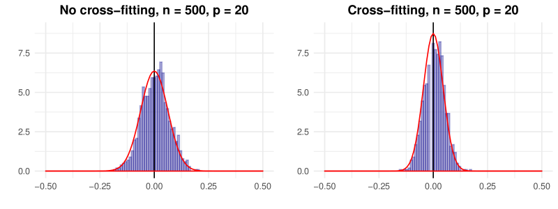
Figure 7: Illustration of efficiency gains due to the use of cross-fitting.

Left panel: Histogram of the centered dml estimator without cross-fitting, $\tilde{\theta}^{nocf}_{0}-\theta_{0}$. $\hat{\theta}^{nocf}_{0}$ is the double machine learning estimator obtained from a sample split into two folds. One fold is used for estimation of the nuisance parameters and the second fold is used for evaluation of the score function and estimation. The empirical distribution can be well-approximated by a normal distribution as indicated by the red curve. Right panel: Histogram of the centered dml estimator with cross-fitting, $\tilde{\theta}_{0}-\theta_{0}$. The estimator is obtained from a split into two folds and application of Algorithm 2 (DML2). In both cases, the estimators are based on estimation of $g_{0}$ and $m_{0}$ with random forests and an orthogonal score function provided in Equation (17). Moreover, exactly the same data sets and exactly the same partitions are used for sample splitting. The empirical distribution of the estimator that is based on cross-fitting exhibits a more pronounced concentration around zero, which reflects the smaller standard errors.

7.8.1 The Role of Cross-Fitting

As mentioned in Section 7.7.1 the use of the cross-fitting Algorithms 1 (DML1) and 2 (DML2) makes it possible to use sample splitting and exploit full efficiency at the same time. To illustrate the superior performance due to cross-fitting, we compare the double machine learning estimator with and without a cross-fitting procedure in the simulation setting that was presented in 4.1. Figure 7 illustrates that efficiency gains can be achieved if the role of the random partitions is swapped in the estimation procedure. Using cross-fitting makes it possible to obtain smaller standard errors for the DML estimator: The empirical distribution of the double machine learning estimator that is based on the cross-fitting Algorithm 2 (DML2) exhibits a more pronounced concentration around zero.

7.8.2 Inference on a Structural Parameter in Key Causal Models

We provide simulation results for double machine learning estimators in the presented key causal models in Figure 8. In a replication of the simulation example in Section 4.1, we show that the confidence intervals for the DML estimator in the partially linear regression model achieves an empirical coverage (= $0.952$) close to the specified level of $1-\alpha=0.95$. The estimator is, again, based on a random forest learner. The corresponding results are presented in the top-left panel of Figure 8.

In a simulated example of a PLIV model, the DML confidence interval that is based on a lasso learner (regr.cv_glmnet of mlr3) achieves a coverage of 95.6%. The underlying data generating process is based on a setting considered in Chernozhukov et al. (2015a) with one instrumental variable. Moreover for simulations of the IRM model, we make use of a DGP of Belloni et al. (2017). The DGP for the IIVM is inspired by a simulation run in Farbmacher et al. (2020). We present the formal DGPs in the Appendix. To perform estimation of the nuisance functions in the interactive models, we employ the regression and classification predictors regr.cv_glmnet and classif.cv_glmnet as provided by the mlr3 package. In all cases, we employ the cross-validated lambda.min choice of the penalty parameter with five folds, in other words, that $\lambda$ value that minimizes the cross-validated mean squared error. Figure 8 shows that the empirical distribution of the centered estimators as obtained in finite sample settings is relatively well-approximated by a normal distribution. In all models the empirical coverage that is achieved by the constructed confidence bands is close to the nominal level.

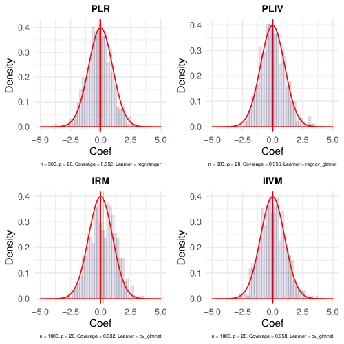
Figure 8: Histogram of double machine learning estimators in key causal models.

The figure shows the histograms of the realizations of the DML estimators in the PLR (top left), PLIV (top right), IRM (bottom left), and IIVM (bottom right) as obtained in $R=500$ independent repetitions. Additional information on the data generating processes and implemented estimators are presented in the main text and the Appendix.

7.8.3 Simultaneous Inference

To verify the finite-sample performance of the implemented methods for simultaneous inference, we perform a small simulation study in a regression setup which is similar as the one used in Bach et al. (2018). We would like to perform valid simultaneous inference on the coefficients $\theta$ in the regression model

$$y_{i}=\beta_{0}+d_{i}^{\prime}\theta+\varepsilon_{i},\quad\quad i=1,\ldots,n,$$ (38)

with $n=1000$ and $p_{1}=42$ regressors. The errors $\varepsilon_{i}$ are normally distributed with $\varepsilon_{i}\sim N(0,\sigma^{2})$ and variance $\sigma^{2}=3$. The regressors $d_{i}$ are generated by a joint normal distribution $d_{i}\sim N(\mu,\Sigma)$ with $\mu=\mathbf{0}$ and $\Sigma_{j,k}=0.5^{|j-k|}$. The model is sparse in that only the first $s=12$ regressors have a non-zero effect on outcome $y_{i}$. The $p_{1}$ coefficients $\theta_{1},\ldots,\theta_{p_{1}}$ are generated as

$$\theta_{j}=\min\left\{\frac{\theta^{\max}}{j^{a}},\theta^{\min}\right\},$$

for $j=1,\ldots,s$ with $\theta^{\max}=9$, $\theta^{min}=0.75$, and $a=0.99$. All other coefficients have values exactly equal to $0$. Estimation of the nuisance components has been performed by using the lasso as provided by regr.cv_glmnet in mlr3.

We report the empirical coverage as achieved by a joint $(1-\alpha)$-confidence interval for all $p_{1}=42$ coefficients and the realized family-wise error rate of the implemented $p$-value adjustments in $R=500$ repetitions in Table 1. The finite sample performance of the Romano-Wolf stepdown procedure that is based on the multiplier bootstrap as well as the classical Bonferroni and Bonferroni-Holm correction are evaluated. Table 1 shows that all methods achieve an empirical FWER close to the specified level of $\alpha=0.1$. In all cases, the double machine learning estimators reject all 12 false null hypotheses in every repetition.

	CI	RW	Bonf	Holm
FWER	0.08	0.11	0.08	0.10
Cor. Rejections	12.00	12.00	12.00	12.00

Table 1: Simulation results, simultaneous inference.

Family-wise error rate (FWER) and average number of correct rejections in a simulation example. CI: Joint confidence interval, RW: Romano-Wolf stepdown correction, Bonf: Bonferroni adjustment, Holm: Bonferroni-Holm correction.

8 Conclusion

In this paper, we provide an overview on the key ingredients and the major structure of the double/debiased machine learning framework as established in Chernozhukov et al. (2018) together with an overview on a collection of structural models. Moreover, we introduce the R package DoubleML that serves as an implementation of the double machine learning approach. A brief simulation study provides insights on the finite sample performance of the double machine learning estimator in the key causal models.

The structure of DoubleML is intended to be flexible with regard to the implemented structural models, the resampling scheme, the machine learning methods and the underlying algorithm, as well as the Neyman-orthogonal scores considered. By providing the R package DoubleML together with its Python twin (Bach et al., 2021), we hope to make double machine learning more accessible to users in practice. Finally, we would like to encourage users to add new structural models, scores and functionalities to the package.

 

9 Appendix

9.1 Computation and Infrastructure

The code in the paper has been executed with DoubleML, version 0.5.2.

The simulation study has been run on a x86_64, darwin17.0 with macos Big Sur … 10.16 system using R version 4.2.2 (2022-10-31). The following packages have been used for estimation:

• DoubleML, version 0.5.2,

• data.table, version 1.14.6,

• mlr3, version 0.14.1,

• mlr3tuning, version 0.17.2,

• mlr3learners, version 0.5.5,

• glmnet, version 4.1-6,

• ranger, version 0.14.1,

• paradox, version 0.11.0,

• foreach, version 1.5.2.

9.2 Suppressed Code Output

Pennsylvania Reemployment Data, Section 7

library(DoubleML)

# Load data as data.table

dt_bonus = fetch_bonus(return_type = "data.table")

dt_bonus

##       inuidur1 female black othrace dep1 dep2 q2 q3 q4 q5 q6 agelt35 agegt54
##    1: 2.890372      0     0       0    0    1  0  0  0  1  0       0       0
##    2: 0.000000      0     0       0    0    0  0  0  0  1  0       0       0
##    3: 3.295837      0     0       0    0    0  0  0  1  0  0       0       0
##    4: 2.197225      0     0       0    0    0  0  1  0  0  0       1       0
##    5: 3.295837      0     0       0    1    0  0  0  0  1  0       0       1
##   ---
## 5095: 2.302585      0     0       0    0    0  0  1  0  0  0       1       0
## 5096: 1.386294      0     0       0    0    1  1  0  0  0  0       0       0
## 5097: 2.197225      0     0       0    0    1  1  0  0  0  0       1       0
## 5098: 1.386294      0     0       0    0    0  0  0  0  1  0       0       1
## 5099: 3.295837      0     0       0    0    0  0  0  1  0  0       0       1
##       durable lusd husd tg
##    1:       0    0    1  0
##    2:       0    1    0  0
##    3:       0    1    0  0
##    4:       0    0    0  1
##    5:       1    1    0  0
##   ---
## 5095:       0    0    0  1
## 5096:       0    0    0  1
## 5097:       0    1    0  0
## 5098:       0    0    0  1
## 5099:       1    1    0  0

obj_dml_data_bonus = DoubleMLData$new(dt_bonus,

                                      y_col = "inuidur1",

                                      d_cols = "tg",

                                      x_cols = c("female", "black", "othrace",

                                                 "dep1", "dep2", "q2", "q3",

                                                 "q4", "q5", "q6", "agelt35",

                                                 "agegt54", "durable", "lusd",

                                                 "husd"))

# Print data backend: Lists main attributes and methods of a DoubleMLData object

obj_dml_data_bonus

# Print data set (output suppressed)

obj_dml_data_bonus$data

##       inuidur1 female black othrace dep1 dep2 q2 q3 q4 q5 q6 agelt35 agegt54
##    1: 2.890372      0     0       0    0    1  0  0  0  1  0       0       0
##    2: 0.000000      0     0       0    0    0  0  0  0  1  0       0       0
##    3: 3.295837      0     0       0    0    0  0  0  1  0  0       0       0
##    4: 2.197225      0     0       0    0    0  0  1  0  0  0       1       0
##    5: 3.295837      0     0       0    1    0  0  0  0  1  0       0       1
##   ---
## 5095: 2.302585      0     0       0    0    0  0  1  0  0  0       1       0
## 5096: 1.386294      0     0       0    0    1  1  0  0  0  0       0       0
## 5097: 2.197225      0     0       0    0    1  1  0  0  0  0       1       0
## 5098: 1.386294      0     0       0    0    0  0  0  0  1  0       0       1
## 5099: 3.295837      0     0       0    0    0  0  0  1  0  0       0       1
##       durable lusd husd tg
##    1:       0    0    1  0
##    2:       0    1    0  0
##    3:       0    1    0  0
##    4:       0    0    0  1
##    5:       1    1    0  0
##   ---
## 5095:       0    0    0  1
## 5096:       0    0    0  1
## 5097:       0    1    0  0
## 5098:       0    0    0  1
## 5099:       1    1    0  0

learner_classif_m = lrn("classif.ranger", num.trees = 500,

                        min.node.size = 2, max.depth = 5)

doubleml_irm_bonus = DoubleMLIRM$new(obj_dml_data_bonus,

                                     ml_g = learner_g,

                                     ml_m = learner_classif_m,

                                     score = "ATE",

                                     dml_procedure = "dml1",

                                     n_folds = 5,

                                     n_rep = 1)

# output suppressed

doubleml_irm_bonus

## ================= DoubleMLIRM Object ==================
##
##
## ------------------ Data summary      ------------------
## Outcome variable: inuidur1
## Treatment variable(s): tg
## Covariates: female, black, othrace, dep1, dep2, q2, q3, q4, q5, q6, agelt35, agegt54, durable, lusd, husd
## Instrument(s):
## No. Observations: 5099
##
## ------------------ Score & algorithm ------------------
## Score function: ATE
## DML algorithm: dml1
##
## ------------------ Machine learner   ------------------
## ml_g: regr.ranger
## ml_m: classif.ranger
##
## ------------------ Resampling        ------------------
## No. folds: 5
## No. repeated sample splits: 1
## Apply cross-fitting: TRUE
##
## ------------------ Fit summary       ------------------
##

Data-backend with multiple treatment variables, Section 7.5

doubleml_data = double_ml_data_from_data_frame(df,

                                               y_col = "y",

                                               d_cols = c("X1", "X2", "X3",

                                                          "X4", "X5", "X6",

                                                          "X7", "X8", "X9",

                                                          "X10"))

## Set treatment variable d to X1.

# suppress output

doubleml_data

## ================= DoubleMLData Object ==================
##
##
## ------------------ Data summary      ------------------
## Outcome variable: y
## Treatment variable(s): X1, X2, X3, X4, X5, X6, X7, X8, X9, X10
## Covariates: X11, X12, X13, X14, X15, X16, X17, X18, X19, X20, X21, X22, X23, X24, X25, X26, X27, X28, X29, X30, X31, X32, X33, X34, X35, X36, X37, X38, X39, X40, X41, X42, X43, X44, X45, X46, X47, X48, X49, X50, X51, X52, X53, X54, X55, X56, X57, X58, X59, X60, X61, X62, X63, X64, X65, X66, X67, X68, X69, X70, X71, X72, X73, X74, X75, X76, X77, X78, X79, X80, X81, X82, X83, X84, X85, X86, X87, X88, X89, X90, X91, X92, X93, X94, X95, X96, X97, X98, X99, X100
## Instrument(s):
## No. Observations: 500

List of externally provided parameters, Section 7.6.1

# Output: parameters after external tuning

# tuned parameters

str(doubleml_plr$params)

## List of 2
##  $ ml_l:List of 10
##   ..$ X1 :List of 1
##   .. ..$ lambda: num 0.09
##   ..$ X2 :List of 1
##   .. ..$ lambda: num 0.085
##   ..$ X3 : NULL
##   ..$ X4 : NULL
##   ..$ X5 : NULL
##   ..$ X6 : NULL
##   ..$ X7 : NULL
##   ..$ X8 : NULL
##   ..$ X9 : NULL
##   ..$ X10: NULL
##  $ ml_m:List of 10
##   ..$ X1 :List of 1
##   .. ..$ lambda: num 0.1
##   ..$ X2 :List of 1
##   .. ..$ lambda: num 0.095
##   ..$ X3 : NULL
##   ..$ X4 : NULL
##   ..$ X5 : NULL
##   ..$ X6 : NULL
##   ..$ X7 : NULL
##   ..$ X8 : NULL
##   ..$ X9 : NULL
##   ..$ X10: NULL

List of internally tuned parameters, Section 7.6.2

# Output: parameters after internal tuning

# access tuning results for target variable "X1"

doubleml_plr$tuning_res$X1

## $ml_l
## $ml_l[[1]]
## $ml_l[[1]]$tuning_result
## $ml_l[[1]]$tuning_result[[1]]
## $ml_l[[1]]$tuning_result[[1]]$tuning_result
##    lambda learner_param_vals  x_domain regr.mse
## 1:    0.1          <list[2]> <list[1]> 10.53451
##
## $ml_l[[1]]$tuning_result[[1]]$tuning_archive
##     lambda regr.mse warnings errors runtime_learners
##  1:  0.100 10.53451        0      0             0.09
##  2:  0.095 10.60720        0      0             0.13
##  3:  0.085 10.76577        0      0             0.08
##  4:  0.055 11.32053        0      0             0.05
##  5:  0.060 11.21736        0      0             0.09
##  6:  0.050 11.42918        0      0             0.03
##  7:  0.075 10.93077        0      0             0.09
##  8:  0.065 11.11709        0      0             0.09
##  9:  0.080 10.84518        0      0             0.09
## 10:  0.070 11.02168        0      0             0.05
## 11:  0.090 10.68576        0      0             0.09
##                                    uhash  x_domain           timestamp batch_nr
##  1: 61330795-44c1-4ee1-bad6-f2698dc3a136 <list[1]> 2023-01-23 14:31:00        1
##  2: b66c7906-5419-4f9b-ab2e-69606b981a57 <list[1]> 2023-01-23 14:31:00        2
##  3: 29522b64-a7c3-4af2-a912-775ff73231ff <list[1]> 2023-01-23 14:31:01        3
##  4: bab2fc04-e6fb-42ee-be7c-df5877f13a37 <list[1]> 2023-01-23 14:31:01        4
##  5: aaed1e89-8e37-42e6-a8ab-1162913ee849 <list[1]> 2023-01-23 14:31:01        5
##  6: ab8fb6de-e141-4296-a992-9e2524bedf3f <list[1]> 2023-01-23 14:31:02        6
##  7: 76c95663-1b05-4353-9ecf-1871592d5466 <list[1]> 2023-01-23 14:31:02        7
##  8: df888d48-9332-408b-8626-6bc3c2a4ead1 <list[1]> 2023-01-23 14:31:02        8
##  9: 2d7dd05c-9291-4323-9463-2bc2330b33e3 <list[1]> 2023-01-23 14:31:02        9
## 10: 49f4f780-c1f2-425a-a64f-d88074434474 <list[1]> 2023-01-23 14:31:03       10
## 11: 101ce484-71ec-4113-bc22-b494ae8d644b <list[1]> 2023-01-23 14:31:03       11
##
## $ml_l[[1]]$tuning_result[[1]]$params
## NULL
##
##
##
## $ml_l[[1]]$params
## $ml_l[[1]]$params[[1]]
## $ml_l[[1]]$params[[1]]$family
## [1] "gaussian"
##
## $ml_l[[1]]$params[[1]]$lambda
## [1] 0.1
##
##
##
##
## $ml_l$params
## $ml_l$params[[1]]
## $ml_l$params[[1]]$family
## [1] "gaussian"
##
## $ml_l$params[[1]]$lambda
## [1] 0.1
##
##
##
##
## $ml_m
## $ml_m[[1]]
## $ml_m[[1]]$tuning_result
## $ml_m[[1]]$tuning_result[[1]]
## $ml_m[[1]]$tuning_result[[1]]$tuning_result
##    lambda learner_param_vals  x_domain  regr.mse
## 1:    0.1          <list[2]> <list[1]> 0.9794034
##
## $ml_m[[1]]$tuning_result[[1]]$tuning_archive
##     lambda  regr.mse warnings errors runtime_learners
##  1:  0.090 0.9798230        0      0             0.09
##  2:  0.055 0.9971462        0      0             0.06
##  3:  0.075 0.9830963        0      0             0.07
##  4:  0.050 1.0045139        0      0             0.06
##  5:  0.100 0.9794034        0      0             0.05
##  6:  0.060 0.9907519        0      0             0.07
##  7:  0.065 0.9869171        0      0             0.02
##  8:  0.095 0.9797396        0      0             0.10
##  9:  0.085 0.9804282        0      0             0.06
## 10:  0.070 0.9848766        0      0             0.07
## 11:  0.080 0.9813190        0      0             0.09
##                                    uhash  x_domain           timestamp batch_nr
##  1: 190137b6-f655-46cd-98ff-624e2abbb06d <list[1]> 2023-01-23 14:31:03        1
##  2: 906bc6e2-2812-4309-aba7-e6ce7063edfb <list[1]> 2023-01-23 14:31:03        2
##  3: aedfaea9-d453-4f90-acaf-87b3e4d1cd9d <list[1]> 2023-01-23 14:31:04        3
##  4: 3ff8fd64-511e-4eec-928f-065cf1e4c16d <list[1]> 2023-01-23 14:31:04        4
##  5: c73d86aa-ec1a-4526-b6e6-4808be903c1f <list[1]> 2023-01-23 14:31:04        5
##  6: 1187c1c0-c9c3-4b7b-90a7-5583709182e7 <list[1]> 2023-01-23 14:31:04        6
##  7: bc144584-327d-4d07-a55c-e9c18b4cd7ba <list[1]> 2023-01-23 14:31:04        7
##  8: f8e269ea-1e20-4718-a2d6-c06cff18b793 <list[1]> 2023-01-23 14:31:05        8
##  9: 880c1487-f0a9-4c99-a52a-d4c2c21047b6 <list[1]> 2023-01-23 14:31:05        9
## 10: 0e28d80b-5d96-404c-bbdd-b0aef5350617 <list[1]> 2023-01-23 14:31:05       10
## 11: 96902fc1-6f1e-47bd-a629-637158bca497 <list[1]> 2023-01-23 14:31:05       11
##
## $ml_m[[1]]$tuning_result[[1]]$params
## NULL
##
##
##
## $ml_m[[1]]$params
## $ml_m[[1]]$params[[1]]
## $ml_m[[1]]$params[[1]]$family
## [1] "gaussian"
##
## $ml_m[[1]]$params[[1]]$lambda
## [1] 0.1
##
##
##
##
## $ml_m$params
## $ml_m$params[[1]]
## $ml_m$params[[1]]$family
## [1] "gaussian"
##
## $ml_m$params[[1]]$lambda
## [1] 0.1

# tuned parameters

str(doubleml_plr$params)

## List of 2
##  $ ml_l:List of 10
##   ..$ X1 :List of 2
##   .. ..$ family: chr "gaussian"
##   .. ..$ lambda: num 0.1
##   ..$ X2 :List of 2
##   .. ..$ family: chr "gaussian"
##   .. ..$ lambda: num 0.1
##   ..$ X3 :List of 2
##   .. ..$ family: chr "gaussian"
##   .. ..$ lambda: num 0.1
##   ..$ X4 :List of 2
##   .. ..$ family: chr "gaussian"
##   .. ..$ lambda: num 0.09
##   ..$ X5 :List of 2
##   .. ..$ family: chr "gaussian"
##   .. ..$ lambda: num 0.07
##   ..$ X6 :List of 2
##   .. ..$ family: chr "gaussian"
##   .. ..$ lambda: num 0.085
##   ..$ X7 :List of 2
##   .. ..$ family: chr "gaussian"
##   .. ..$ lambda: num 0.085
##   ..$ X8 :List of 2
##   .. ..$ family: chr "gaussian"
##   .. ..$ lambda: num 0.08
##   ..$ X9 :List of 2
##   .. ..$ family: chr "gaussian"
##   .. ..$ lambda: num 0.09
##   ..$ X10:List of 2
##   .. ..$ family: chr "gaussian"
##   .. ..$ lambda: num 0.075
##  $ ml_m:List of 10
##   ..$ X1 :List of 2
##   .. ..$ family: chr "gaussian"
##   .. ..$ lambda: num 0.1
##   ..$ X2 :List of 2
##   .. ..$ family: chr "gaussian"
##   .. ..$ lambda: num 0.095
##   ..$ X3 :List of 2
##   .. ..$ family: chr "gaussian"
##   .. ..$ lambda: num 0.095
##   ..$ X4 :List of 2
##   .. ..$ family: chr "gaussian"
##   .. ..$ lambda: num 0.095
##   ..$ X5 :List of 2
##   .. ..$ family: chr "gaussian"
##   .. ..$ lambda: num 0.1
##   ..$ X6 :List of 2
##   .. ..$ family: chr "gaussian"
##   .. ..$ lambda: num 0.1
##   ..$ X7 :List of 2
##   .. ..$ family: chr "gaussian"
##   .. ..$ lambda: num 0.1
##   ..$ X8 :List of 2
##   .. ..$ family: chr "gaussian"
##   .. ..$ lambda: num 0.1
##   ..$ X9 :List of 2
##   .. ..$ family: chr "gaussian"
##   .. ..$ lambda: num 0.1
##   ..$ X10:List of 2
##   .. ..$ family: chr "gaussian"
##   .. ..$ lambda: num 0.1

9.3 Additional Data Generating Processes, Simulation Study

Data generating process for PLIV simulation

The DGP is based on Chernozhukov et al. (2015a) and defined as

$$\begin{aligned} z_{i}&=\Pi x_{i}+\zeta_{i},\\ d_{i}&=x_{i}^{\prime}\gamma+z_{i}^{\prime}\delta+u_{i},\\ y_{i}&=\alpha d_{i}+x_{i}^{\prime}\beta+\varepsilon_{i},\end{aligned}$$ (39)

with

$$\left(\begin{matrix}\varepsilon_{i}\\ u_{i}\\ \zeta_{i}\\ x_{i}\end{matrix}\right)\sim\mathcal{N}\left(0,\left(\begin{matrix}1&0.6&0&0\\ 0.6&1&0&0\\ 0&0&0.25I_{p_{n}^{z}}&0\\ 0&0&0&\Sigma\end{matrix}\right)\right)$$

where $\Sigma$ is a $p^{x}_{n}\times p^{x}_{n}$ matrix with entries $\Sigma_{kj}=0.5^{|k-j|}$ and $I_{p_{n}^{z}}$ is an identity matrix with dimension $p_{n}^{z}\times p_{n}^{z}$. $\beta=\gamma$ is a $p^{x}_{n}$-vector with entries $\beta=\frac{1}{j^{2}}$ and $\Pi=(I_{p_{n}^{z}},0_{p_{n}^{z}\times(p_{n}^{x}-p_{n}^{z})})$. In the simulation example, we have one instrument, i.e., $p^{z}_{n}=1$ and $p^{x}_{n}=20$ regressors $x_{i}$. In the simulation study, data sets with $n=500$ observations are generated in $R=500$ independent repetitions.

Data generating process for IRM simulation

The DGP is based on a simulation study in Belloni et al. (2017) and defined as

$$\begin{aligned} d_{i}&=1\left\{\frac{\exp(c_{d}x_{i}^{\prime}\beta)}{1+\exp(c_{d}x_{i}^{\prime}\beta)}>v_{i}\right\},&&v_{i}\sim\mathcal{U}(0,1),\\ y_{i}&=\theta d_{i}+c_{y}x_{i}^{\prime}\beta d_{i}+\zeta_{i},&&\zeta_{i}\sim\mathcal{N}(0,1),\end{aligned}$$ (40)

with covariates $x_{i}\sim\mathcal{N}(0,\Sigma)$ where $\Sigma$ is a matrix with entries $\Sigma_{kj}=0.5^{|k-j|}$. $\beta$ is a $p_{x}$-dimensional vector with entries $\beta_{j}=\frac{1}{j^{2}}$ and the constants $c_{y}$ and $c_{d}$ are determined as

$$c_{y}=\sqrt{\frac{R_{y}^{2}}{(1-R_{y}^{2})\beta^{\prime}\Sigma\beta}},\qquad c_{d}=\sqrt{\frac{(\pi^{2}/3)R_{d}^{2}}{(1-R_{d}^{2})\beta^{\prime}\Sigma\beta}}.$$

We set the values of $R_{y}^{2}=0.5$ and $R_{d}^{2}=0.5$ and consider a setting with $n=1000$ and $p=20$. Data generation and estimation have been performed in $R=500$ independent replications.

Data generating process for IIVM simulation

The DGP is defined as

$$\begin{aligned} d_{i}&=1\left\{\alpha_{x}Z+v_{i}>0\right\},\\ y_{i}&=\theta d_{i}+x_{i}^{\prime}\beta+u_{i},\end{aligned}$$ (41)

with $Z\sim\text{Bernoulli}(0.5)$ and

$$\left(\begin{matrix}u_{i}\\ v_{i}\end{matrix}\right)\sim\mathcal{N}\left(0,\left(\begin{matrix}1&0.3\\ 0.3&1\end{matrix}\right)\right).$$

The covariates are drawn from a multivariate normal distribution with $x_{i}\sim\mathcal{N}(0,\Sigma)$ with entries of the matrix $\Sigma$ being $\Sigma_{kj}=0.5^{|j-k|}$ and $\beta$ being a $p_{x}$-dimensional vector with $\beta_{j}=\frac{1}{\beta^{2}}$. The data generating process is inspired by a process used in a simulation in Farbmacher et al. (2020). In the simulation study, data sets with $n=1000$ observations and $p_{x}=20$ confounding variables $x_{i}$ have been generated in $R=500$ independent repetitions.

References

- Angrist and Pischke (2009) Joshua D Angrist and Jörn-Steffen Pischke. Mostly harmless econometrics: An empiricist’s companion. Princeton university press, 2009.
- Athey et al. (2019) Susan Athey, Julie Tibshirani, and Stefan Wager. Generalized random forests. The Annals of Statistics, 47(2):1148–1178, 2019. URL https://cran.r-project.org/package=grf.
- Bach et al. (2018) Philipp Bach, Victor Chernozhukov, and Martin Spindler. Valid simultaneous inference in high-dimensional settings (with the hdm package for r). arXiv preprint arXiv:1809.04951, 2018.
- Bach et al. (2021) Philipp Bach, Victor Chernozhukov, Malte S Kurz, and Martin Spindler. DoubleML – An object-oriented implementation of double machine learning in Python. arXiv preprint arXiv:2104.03220, 2021.
- Becker et al. (2020) Marc Becker, Michel Lang, Jakob Richter, Bernd Bischl, and Daniel Schalk. mlr3tuning: Tuning for ’mlr3’, 2020. URL https://CRAN.R-project.org/package=mlr3tuning. R package version 0.7.0.
- Becker et al. (2021) Marc Becker, Martin Binder, Bernd Bischl, Michel Lang, Florian Pfisterer, Nicholas G. Reich, Jakob Richter, Patrick Schratz, and Raphael Sonabend. mlr3 book, 03 2021. URL https://mlr3book.mlr-org.com.
- Belloni et al. (2011) Alexandre Belloni, Victor Chernozhukov, and Christian Hansen. Inference for high-dimensional sparse econometric models. In Advances in Economics and Econometrics. 10th World Congress of Econometric Society. August 2010., pages III:245–295. 2011.
- Belloni et al. (2012) Alexandre Belloni, Daniel Chen, Victor Chernozhukov, and Christian Hansen. Sparse models and methods for optimal instruments with an application to eminent domain. Econometrica, 80:2369–2429, 2012. Arxiv, 2010.
- Belloni et al. (2014a) Alexandre Belloni, Victor Chernozhukov, and Kengo Kato. Uniform post-selection inference for least absolute deviation regression and other z-estimation problems. Biometrika, 102(1):77–94, Dec 2014a. URL http://dx.doi.org/10.1093/biomet/asu056.
- Belloni et al. (2014b) Alexandre Belloni, Victor Chernozhukov, and Lie Wang. Pivotal estimation via square-root lasso in nonparametric regression. The Annals of Statistics, 42(2):757–788, 2014b.
- Belloni et al. (2014c) Alexandre Belloni, Victor Chernozukov, and Christian Hansen. Inference on treatment effects after selection among high-dimensional controls. The Review of Economic Studies, 81(2 (287)):608–650, 2014c. URL http://www.jstor.org/stable/43551575.
- Belloni et al. (2017) Alexandre Belloni, Victor Chernozhukov, Ivan Fernández-Val, and Christian Hansen. Program evaluation and causal inference with high-dimensional data. Econometrica, 85(1):233–298, 2017.
- Belloni et al. (2018) Alexandre Belloni, Victor Chernozhukov, Denis Chetverikov, and Ying Wei. Uniformly valid post-regularization confidence regions for many functional parameters in z-estimation framework. Annals of Statistics, 46(6B):3643–3675, 2018.
- Bia et al. (2020) Michela Bia, Martin Huber, and Lukáš Lafférs. Double machine learning for sample selection models. arXiv preprint arXiv:2012.00745, 2020.
- Bickel et al. (1993) Peter J Bickel, Chris AJ Klaassen, Ya’acov Ritov, and Jon A Wellner. Efficient and adaptive estimation for semiparametric models, volume 4. Johns Hopkins University Press Baltimore, 1993.
- Bilias (2000) Yannis Bilias. Sequential testing of duration data: the case of the Pennsylvania ‘reemployment bonus’ experiment. Journal of Applied Econometrics, 15(6):575–594, 2000.
- Bodory and Huber (2020) Hugo Bodory and Martin Huber. causalweight: Estimation Methods for Causal Inference Based on Inverse Probability Weighting, 2020. URL https://CRAN.R-project.org/package=causalweight. R package version 1.0.0.
- Breiman (1996) Leo Breiman. Stacked regressions. Machine learning, 24(1):49–64, 1996.
- Bühlmann and Van De Geer (2011) Peter Bühlmann and Sara Van De Geer. Statistics for high-dimensional data: methods, theory and applications. Springer Science & Business Media, 2011.
- Bühlmann and van de Geer (2015) Peter Bühlmann and Sara van de Geer. High-dimensional inference in misspecified linear models. Electronic Journal of Statistics, 9(1):1449–1473, 2015.
- Chang (2020a) Neng-Chieh Chang. Double/debiased machine learning for difference-in-differences models. The Econometrics Journal, 23(2):177–191, 2020a.
- Chang (2020b) Winston Chang. R6: Encapsulated classes with reference semantics, 2020b. URL https://CRAN.R-project.org/package=R6. R package version 2.5.0.
- Chernozhukov et al. (2013) Victor Chernozhukov, Denis Chetverikov, and Kengo Kato. Gaussian approximations and multiplier bootstrap for maxima of sums of high-dimensional random vectors. The Annals of Statistics, 41(6):2786–2819, 2013.
- Chernozhukov et al. (2014) Victor Chernozhukov, Denis Chetverikov, and Kengo Kato. Gaussian approximation of suprema of empirical processes. The Annals of Statistics, 42(4):1564–1597, 2014.
- Chernozhukov et al. (2015a) Victor Chernozhukov, Christian Hansen, and Martin Spindler. Post-selection and post-regularization inference in linear models with many controls and instruments. American Economic Review, 105(5):486–90, 2015a.
- Chernozhukov et al. (2015b) Victor Chernozhukov, Christian Hansen, and Martin Spindler. Valid post-selection and post-regularization inference: An elementary, general approach. Annual Review of Economics, 7(1):649–688, 2015b. URL https://doi.org/10.1146/annurev-economics-012315-015826.
- Chernozhukov et al. (2016) Victor Chernozhukov, Chris Hansen, and Martin Spindler. hdm: High-Dimensional Metrics. The R Journal, 8(2):185–199, 2016. URL https://CRAN.R-project.org/package=hdm.
- Chernozhukov et al. (2018) Victor Chernozhukov, Denis Chetverikov, Mert Demirer, Esther Duflo, Christian Hansen, Whitney Newey, and James Robins. Double/debiased machine learning for treatment and structural parameters. The Econometrics Journal, 21(1):C1–C68, 2018. URL https://onlinelibrary.wiley.com/doi/abs/10.1111/ectj.12097.
- Coyle (2021) Jeremy Coyle. tmle3: The Extensible TMLE Framework, 2021. URL https://github.com/tlverse/tmle3. R package version 0.2.0.
- Coyle et al. (2021) Jeremy Coyle, Nima Hejazi, Ivana Malenica, Rachael Phillips, and Oleg Sofrygin. sl3: Pipelines for Machine Learning and Super Learning, 2021. URL https://github.com/tlverse/sl3. R package version 1.4.4.
- Cunningham (2021) Scott Cunningham. Causal inference. In Causal Inference. Yale University Press, 2021.
- Dezeure et al. (2015) Ruben Dezeure, Peter Bühlmann, Lukas Meier, and Nicolai Meinshausen. High-dimensional inference: Confidence intervals, p-values and R-software hdi. Statistical Science, 30(4):533–558, 2015.
- Dowle and Srinivasan (2020) Matt Dowle and Arun Srinivasan. data.table: Extension of ‘data.frame‘, 2020. URL https://CRAN.R-project.org/package=data.table. R package version 1.13.2.
- Dudoit and van der Laan (2005) Sandrine Dudoit and Mark J van der Laan. Asymptotics of cross-validated risk estimation in estimator selection and performance assessment. Statistical methodology, 2(2):131–154, 2005.
- Farbmacher et al. (2020) Helmut Farbmacher, Raphael Guber, and Sven Klaassen. Instrument validity tests with causal forests. Journal of Business & Economic Statistics, pages 1–10, 2020.
- Farbmacher et al. (2022) Helmut Farbmacher, Martin Huber, Lukáš Lafférs, Henrika Langen, and Martin Spindler. Causal mediation analysis with double machine learning. The Econometrics Journal, 25(2):277–300, 01 2022. ISSN 1368-4221. doi: 10.1093/ectj/utac003. URL https://doi.org/10.1093/ectj/utac003.
- Farrell et al. (2021) Max H Farrell, Tengyuan Liang, and Sanjog Misra. Deep neural networks for estimation and inference. Econometrica, 89(1):181–213, 2021.
- Friedman et al. (2010) Jerome Friedman, Trevor Hastie, and Robert Tibshirani. Regularization paths for generalized linear models via coordinate descent. Journal of Statistical Software, 33(1):1–22, 2010. URL http://www.jstatsoft.org/v33/i01.
- Gruber and van der Laan (2012) Susan Gruber and Mark J. van der Laan. tmle: An R package for targeted maximum likelihood estimation. Journal of Statistical Software, 51(13):1–35, 2012. URL https://www.jstatsoft.org/v51/i13/. doi:10.18637/jss.v051.i13.
- Imbens and Angrist (1994) Guido W. Imbens and Joshua D. Angrist. Identification and estimation of local average treatment effects. Econometrica, 62(2):467–475, 1994. URL http://www.jstor.org/stable/2951620.
- Javanmard and Montanari (2014) Adel Javanmard and Andrea Montanari. Hypothesis testing in high-dimensional regression under the gaussian random design model: Asymptotic theory. IEEE Transactions on Information Theory, 60(10):6522–6554, 2014.
- Javanmard and Montanari (2018) Adel Javanmard and Andrea Montanari. Debiasing the lasso: Optimal sample size for gaussian designs. The Annals of Statistics, 46(6A):2593–2622, 2018.
- Klaassen (1987) Chris AJ Klaassen. Consistent estimation of the influence function of locally asymptotically linear estimators. The Annals of Statistics, 15(4):1548–1562, 1987.
- Knaus (2020) Michael C Knaus. Double machine learning based program evaluation under unconfoundedness. arXiv preprint arXiv:2003.03191, 2020. URL https://github.com/MCKnaus/causalDML.
- Knaus (2021) Michael C Knaus. A double machine learning approach to estimate the effects of musical practice on student’s skills. Journal of the Royal Statistical Society: Series A (Statistics in Society), 184(1):282–300, 2021. URL https://github.com/MCKnaus/dmlmt.
- Kurz (2021) Malte S Kurz. Distributed double machine learning with a serverless architecture. In Companion of the ACM/SPEC International Conference on Performance Engineering, ICPE ’21, pages 27–33, New York, NY, USA, 2021. Association for Computing Machinery. doi: 10.1145/3447545.3451181.
- Lang et al. (2019) Michel Lang, Martin Binder, Jakob Richter, Patrick Schratz, Florian Pfisterer, Stefan Coors, Quay Au, Giuseppe Casalicchio, Lars Kotthoff, and Bernd Bischl. mlr3: A modern object-oriented machine learning framework in R. Journal of Open Source Software, 2019. URL https://joss.theoj.org/papers/10.21105/joss.01903.
- Lang et al. (2020a) Michel Lang, Quay Au, Stefan Coors, and Patrick Schratz. mlr3learners: Recommended learners for ’mlr3’, 2020a. URL https://CRAN.R-project.org/package=mlr3learners. R package version 0.4.3.
- Lang et al. (2020b) Michel Lang, Bernd Bischl, Jakob Richter, Xudong Sun, and Martin Binder. paradox: Define and work with parameter spaces for complex algorithms, 2020b. URL https://CRAN.R-project.org/package=paradox. R package version 0.7.1.
- Microsoft Research (2019) Microsoft Research. EconML: A Python package for ML-based heterogeneous treatment effects estimation. https://github.com/microsoft/EconML, 2019. Version 0.x.
- Newey (1994) Whitney Newey. The asymptotic variance of semiparametric estimators. Econometrica, 62(6):1349–1382, 1994.
- Neyman (1959) Jerzy Neyman. Optimal asymptotic tests of composite hypotheses. In Ulf Grenander, editor, Probability and Statistics, pages 213–234. Almqvist & Wiksell, 1959.
- Pedregosa et al. (2011) Fabian Pedregosa, Gaël Varoquaux, Alexandre Gramfort, Vincent Michel, Bertrand Thirion, Olivier Grisel, Mathieu Blondel, Peter Prettenhofer, Ron Weiss, Vincent Dubourg, Jake Vanderplas, Alexandre Passos, David Cournapeau, Matthieu Brucher, Matthieu Perrot, and Édouard Duchesnay. Scikit-learn: Machine learning in python. Journal of Machine Learning Research, 12(85):2825–2830, 2011. URL http://jmlr.org/papers/v12/pedregosa11a.html.
- Permutt and Hebel (1989) Thomas Permutt and J Richard Hebel. Simultaneous-equation estimation in a clinical trial of the effect of smoking on birth weight. Biometrics, 45:619–622, 1989.
- Polley et al. (2021) Eric Polley, Erin LeDell, Chris Kennedy, and Mark van der Laan. SuperLearner: Super Learner Prediction, 2021. URL https://CRAN.R-project.org/package=SuperLearner. R package version 2.0-28.
- Poterba et al. (1994) James M Poterba, Steven F Venti, and David A Wise. 401 (k) plans and tax-deferred saving. Studies in the Economics of Aging, pages 105–142, 1994.
- Poterba et al. (1995) James M Poterba, Steven F Venti, and David A Wise. Do 401 (k) contributions crowd out other personal saving? Journal of Public Economics, 58(1):1–32, 1995.
- R Core Team (2020) R Core Team. R: A language and environment for statistical computing. R Foundation for Statistical Computing, Vienna, Austria, 2020. URL https://www.R-project.org/.
- Robins and Rotnitzky (1995) James M Robins and Andrea Rotnitzky. Semiparametric efficiency in multivariate regression models with missing data. Journal of the American Statistical Association, 90(429):122–129, 1995.
- Robinson (1988) Peter M Robinson. Root-n-consistent semiparametric regression. Econometrica, 56(4):931–954, 1988.
- Romano and Wolf (2005a) Joseph P Romano and Michael Wolf. Exact and approximate stepdown methods for multiple hypothesis testing. Journal of the American Statistical Association, 100(469):94–108, 2005a.
- Romano and Wolf (2005b) Joseph P Romano and Michael Wolf. Stepwise multiple testing as formalized data snooping. Econometrica, 73(4):1237–1282, 2005b.
- Romano and Wolf (2016) Joseph P Romano and Michael Wolf. Efficient computation of adjusted p-values for resampling-based stepdown multiple testing. Statistics & Probability Letters, 113:38–40, 2016.
- Schick (1986) Anton Schick. On asymptotically efficient estimation in semiparametric models. The Annals of Statistics, 14(3):1139–1151, 1986.
- Sonabend and Schratz (2020) Raphael Sonabend and Patrick Schratz. mlr3extralearners: Extra learners For mlr3, 2020. R package version 0.3.0.9000.
- Tibshirani et al. (2020) Julie Tibshirani, Susan Athey, and Stefan Wager. grf: Generalized random forests, 2020. URL https://CRAN.R-project.org/package=grf. R package version 1.2.0.
- van de Geer et al. (2014) Sara van de Geer, Peter Bühlmann, Ya’acov Ritov, and Ruben Dezeure. On asymptotically optimal confidence regions and tests for high-dimensional models. Annals of Statistics, 42(3):1166–1202, 06 2014. doi: 10.1214/14-AOS1221. URL https://doi.org/10.1214/14-AOS1221.
- Van der Laan and Rose (2011) Mark J Van der Laan and Sherri Rose. Targeted learning: causal inference for observational and experimental data. Springer Science & Business Media, 2011.
- Van der Laan et al. (2007) Mark J Van der Laan, Eric C Polley, and Alan E Hubbard. Super learner. Statistical applications in genetics and molecular biology, 6(1), 2007.
- van der Laan et al. (2022) MJ van der Laan, JR Coyle, NS Hejazi, I Malenica, RV Phillips, and AE Hubbard. Targeted learning in R: Causal data science with the tlverse software ecosystem, 2022. URL https://tlverse.org/tlverse-handbook/index.html.
- Van der Vaart (2000) Aad W Van der Vaart. Asymptotic statistics, volume 3. Cambridge university press, 2000.
- Wickham (2019) Hadley Wickham. Advanced R. CRC press, 2019.
- Wolpert (1992) David H Wolpert. Stacked generalization. Neural networks, 5(2):241–259, 1992.
- Wright and Ziegler (2017) Marvin N. Wright and Andreas Ziegler. ranger: A fast implementation of random forests for high dimensional data in C++ and R. Journal of Statistical Software, 77(1):1–17, 2017. doi: 10.18637/jss.v077.i01.
- Wright (1928) Philip G Wright. Tariff on animal and vegetable oils. Macmillan Company, New York, 1928.
- Zhang and Zhang (2014) Cun-Hui Zhang and Stephanie S. Zhang. Confidence intervals for low dimensional parameters in high dimensional linear models. Journal of the Royal Statistical Society: Series B (Statistical Methodology), 76(1):217–242, 2014. doi: 10.1111/rssb.12026. URL https://rss.onlinelibrary.wiley.com/doi/abs/10.1111/rssb.12026.
- Zheng and Laan (2011) Wenjing Zheng and Mark J Laan. Cross-validated targeted minimum-loss-based estimation. In Targeted Learning, pages 459–474. Springer, 2011.
- Zhong and Naimi (2021) Yongqi Zhong and Ashley Naimi. AIPW: Augmented Inverse Probability Weighting (AIPW) for binary exposure, 2021. URL https://github.com/yqzhong7/AIPW. R package version 0.6.3.1.