Influence of thermal fluctuations on active diffusion at large Péclet numbers

Abstract

Wavelet Monte Carlo dynamics simulations are used to study the dynamics of passive particles in the presence of microswimmers, taking account of the often-omitted thermal motion alongside the hydrodynamic flows generated by the swimmers. Although the Péclet numbers considered are large, we find the thermal motion to have a significant effect on the dynamics of our passive particles, and can be included as a decorrelation factor in the velocity autocorrelation with a decay time proportional to the Péclet number. Similar decorrelation factors come from swimmer rotations, e.g. run and tumble motion, and apply to both entrainment and far field loop contributions. These decorrelation factors lead to active diffusivity having a weak apparent power law close to $\mathrm{Pe}^{0.2}$ for small tracer-like particles at Péclet numbers appropriate for E. coli swimmers at room temperature. Meanwhile, the reduced hydrodynamic response of large particles to nearby forces has a corresponding reduction in active diffusivity in that regime. Together, they lead to a non-monotonic dependence of active diffusivity on particle size that can shed light on similar behaviour observed in experiments by Patteson et al.

I Introduction

The influence of microswimmers, e.g. algae or bacteria, on the dynamics of passive particles has received much attention since Wu and Libchaber first observed enhanced diffusion of spherical beads suspended in a soap film with E. coli Wu and Libchaber (2000). The subsequent research into the swimmer-induced diffusion, often simply called ‘active diffusion’, of colloids or infinitesimal tracer particles has spanned experiments Soni et al. (2003); Leptos et al. (2009); Miño et al. (2011); Kurtuldu et al. (2011); Valeriani et al. (2011); Miño et al. (2013); Jepson et al. (2013); Jeanneret et al. (2016); Mathijssen, Jeanneret, and Polin (2018), simulations Valeriani et al. (2011); Underhill, Hernandez-Ortiz, and Graham (2008); Molina and Yamamoto (2014); Morozov and Marenduzzo (2014); Krafnick and García (2015); Krishnamurthy and Subramanian (2015); de Graaf and Stenhammar (2017); Shum and Yeomans (2017); Harder and Cacciuto (2018) and analytic calculations Miño et al. (2013); Mathijssen, Jeanneret, and Polin (2018); Dunkel et al. (2010); Thiffeault and Childress (2010); Eckhardt and Zammert (2012); Mathijssen, Pushkin, and Yeomans (2015); Thiffeault (2015); Suma, Cugliandolo, and Gonnella (2016); Burkholder and Brady (2017); Yasuda, Okamoto, and Komura (2017); Mueller and Thiffeault (2017), each in both 3 and (quasi-)2 dimensions.

While the precise results vary with the details of each system, all find the passive particles to exhibit enhanced motion over and above their own thermally-driven Brownian motion. This swimmer-induced motion is super-diffusive on the time-scales of interactions with passing swimmers, and diffusive thereafter Miño et al. (2013); Krafnick and García (2015).

Until recently the size of the passive particles has received little attention, with a range of sizes used across the literature but typically a constant size within a given study. Nevertheless one can identify several relevant properties that change with particle size: the thermal diffusivity and by extension the Péclet number $\mathrm{Pe}$ (defined as the ratio of advective and diffusive transport rates); the range of steric interactions with swimmers; and the near-field hydrodynamic response to swimmers Faxén (1922); Durlofsky, Brady, and Bossis (1987); Rotne and Prager (1969); Yamakawa (1970).

The influence of Péclet number was included in a theoretical study by Kasyap et al. Kasyap, Koch, and Wu (2014), which predicts a peak in swimmer-induced diffusivities at moderate $\mathrm{Pe}$, rising from 0 at $\mathrm{Pe}=0$ (corresponding to infinitesimal tracers) and limiting to a finite value as $\mathrm{Pe}\rightarrow\infty$. While this work accounted for particle size in the passive particles’ thermal motion, they were hydrodynamically coupled to the swimmers by the (unregularised) Oseen tensor so that they were treated as point particles for hydrodynamic purposes. Their results might therefore not be expected to quantitatively match real systems except when at small $\mathrm{Pe}$.

Shum and Yeomans have performed detailed boundary element simulations of single swimmer-passive interactions with a wide range of passive particle sizes, neglecting all thermal motion Shum and Yeomans (2017). From these results they obtained the dilute limit active diffusivity by integrating over impact parameters. In doing so they found a non-trivial dependence on the ratio of passive and active particle size, with a maximum active diffusivity for similarly sized particles when using a squirmer type swimmer model, but a minimum instead with bacteria models.

An experimental investigation of passive particle size active systems of E. coli was conducted by Patteson et al. Patteson et al. (2016), who found a non-monotonic variation in active diffusivity, peaking when the swimmer and passive particle sizes are similar. This runs counter to the results for Shum and Yeomans’ bacterial model. This non-monotonicity suggests regimes where different particle sizes are dominated by different physics. Since thermal diffusivity rises rapidly as particles get smaller, $D\sim R^{-1}$, we hypothesise this is important and will study simulations of analogous systems with this in mind.

It is notable that thermal fluctuations have usually been omitted from simulations of microswimmers on the basis that swimmer Péclet numbers are generally much greater than unity. Work that has included thermal motion has done so in a hydrodynamically decoupled way Krishnamurthy and Subramanian (2015). While this can capture some of the physics, the hydrodynamic coupling is required to provide the correct relative thermal motion.

To elucidate the potential importance of thermal fluctuations we draw parallels to Taylor dispersion in pipes containing a steady shear flow Taylor (1953); Mathijssen, Jeanneret, and Polin (2018). In the absence of thermal fluctuations passive particles are carried parallel to the pipe axis at constant speed which is fastest at the centre of the pipe. Thermal fluctuations allow particles to cross stream lines, with a corresponding change of advective velocity, leading to dispersion of particles in the stream direction. Although the microswimmer flow fields are more complex, the crossing of stream lines is still expected to disperse advective motion, and will therefore have some influence on the active diffusion of passive particles, even if the Brownian motion itself is small. In the slightly more limited context of particle entrainment, this effect has been seen to lead to a non-monotonic distribution of entrainment jump sizes with particle size Mathijssen, Jeanneret, and Polin (2018).

Another reason for the limited microswimmer work including thermal fluctuations is the great computational expense required to include the correct hydrodynamics of thermal fluctuations, which is a challenge well known to the polymer community where it has spawned a wide range of simulation algorithms Pham et al. (2009); Jain et al. (2012); Dyer and Ball (2017). Here we make use of the recently developed Wavelet Monte Carlo dynamics (WMCD) algorithm to include hydrodynamically coupled thermal fluctuations efficiently Dyer and Ball (2017); Dyer (2019).

After setting out the hydrodynamic theory and simulation details in Sections II and III, we will demonstrate the validity of using WMCD for active systems in Section IV, where we use trajectories of passive particles in the flow of a swimmer on an infinite straight path as a test case. We then study the dynamics of passive particles in dilute mixtures of swimmers, looking in detail at the role of particle size and temperature on the velocity autocorrelation and active diffusivity in Sections V and VI respectively. In doing so we find we can include the effect of all relevant time scales through exponential decay factors in the velocity autocorrelation, allowing us to construct an ansatz function that successfully captures the complex behaviour seen in the active diffusivity.

II Theory

II.1 Active diffusivity

The total diffusivity of a particle can be split into thermal and active contributions as

$$D=D_{T}+D_{A}.$$ (1)

The thermal diffusivity for a sphere of radius $a$ in fluid of viscosity $\eta$ is given by the well-known Stokes-Einstein relation, which in a periodic cubic box of side length $L$ is corrected to

$$D_{T}=\frac{k_{B}T}{6\pi\eta a}\left(1-2.837\frac{a}{L}\right)$$ (2)

to first order Dünweg and Kremer (1993).

Rather than thermal fluctuations, the active diffusivity $D_{A}$ is driven by hydrodynamic and steric interactions with active particles in the system, and can itself be written as the sum of those contributions Pushkin and Yeomans (2013). To simplify data analysis we will not include steric interactions in this work so $D_{A}$ is purely hydrodynamic.

Regardless of its contributions, the active diffusivity can be expressed in terms of the velocity autocorrelation

$$C_{vv}(t)=\langle\textbf{v}(t)\cdot\textbf{v}(0)\rangle$$ (3)

via the Green-Kubo relation Green (1954); Kubo (1957)

$$D_{A}=\frac{1}{3}\int\limits_{0^{+}}^{\infty}dt\,C_{vv}(t).$$ (4)

The lower limit $0^{+}$ denotes time $t\rightarrow 0$ from above, such that the thermal contribution is excluded when working in the overdamped limit (see the next section). In practice this means the $t=0$ value we use in our data is extrapolated back from data at small but finite $t$.

II.2 Equations of motion

Working on time scales where thermal fluctuations can be considered instantaneous, or equivalently on time scales longer than the fluid relaxation time, leads to the overdamped Langevin equations for translational (superscript T) and rotational (R) velocities:

$$\textbf{v}_{i}=\sum\limits_{j}\bm{\mathcal{G}}^{\mathrm{TT}}_{ij}\cdot\textbf{F}_{j}+\sum\limits_{j}\bm{\mathcal{G}}^{\mathrm{TR}}_{ij}\cdot\bm{\Gamma}_{j}+\bm{\xi}_{i}$$ (5)

and

$$\bm{\omega}_{i}=\sum\limits_{j}\bm{\mathcal{G}}^{\mathrm{RT}}_{ij}\cdot\textbf{F}_{j}+\sum\limits_{j}\bm{\mathcal{G}}^{\mathrm{RR}}_{ij}\cdot\bm{\Gamma}_{j}+\bm{\Xi}_{i},$$ (6)

where $\textbf{F}_{j}$ and $\bm{\Gamma}_{j}$ denote the force and torque at $\textbf{r}_{j}$, which may or may not be located on a particle. In this work $i$ will correspond to a particle, while the sum over $j$ corresponds to a sum over the swimmer forces described in Section III.2. We will not apply any point torques, so $\bm{\Gamma}_{j}=0$ for all $j$, but their inclusion here is useful for introducing the rotational mobility tensors which will be needed for correlations between the thermal fluctuations, $\bm{\xi}$ and $\bm{\Xi}$.

The Lorentz reciprocal theorem links the TR and RT tensors by the transpose Happel and Brenner (1973)

$$\bm{\mathcal{G}}^{\mathrm{TR}}_{ij} = \left(\bm{\mathcal{G}}^{\mathrm{RT}}_{ji}\right)^{\textsf{T}}.$$ (7)

For spheres, the unregularised versions of these tensors are to leading order in $1/r$:

$$\bm{\mathcal{G}}^{\mathrm{TT}}_{ij} = \frac{\delta_{ij}}{6\pi\eta a_{i}}\textbf{I}+\frac{1-\delta_{ij}}{8\pi\eta r_{ij}}\,(\textbf{I}+\hat{\textbf{r}}_{ij}\otimes\hat{\textbf{r}}_{ij}),$$ (8)

$$\bm{\mathcal{G}}^{\mathrm{RT}}_{ij} = \delta_{ij}\,\textbf{0}-\frac{1-\delta_{ij}}{8\pi\eta r_{ij}^{2}}\,[\hat{\textbf{r}}_{ij}]_{\times},$$ (9)

$$\bm{\mathcal{G}}^{\mathrm{RR}}_{ij} = \frac{\delta_{ij}}{8\pi\eta a_{i}^{3}}\textbf{I}+\frac{1-\delta_{ij}}{16\pi\eta r_{ij}^{3}}\,(3\hat{\textbf{r}}_{ij}\otimes\hat{\textbf{r}}_{ij}-\textbf{I}),$$ (10)

where $a_{i}$ is the radius of particle $i$, $\delta_{ij}$ is the Kronecker-delta and $[\hat{\textbf{r}}]_{\times}$ is the skew-symmetric tensor expressed as $\varepsilon_{abc}\hat{r}_{b}$ in index notation.

The mobility tensors used in this work are those that appear in Wavelet Monte Carlo Dynamics (WMCD) Dyer and Ball (2017); Dyer (2019), described below, which smoothly bridge the large $r$ and $\delta_{ij}$ terms. Although reached in a completely different way, they closely approximate the tensors obtained by using Faxén’s laws to sum the fluid flow over the particle surface Durlofsky, Brady, and Bossis (1987).

Finally, the fluctuation dissipation theorem gives Kubo (1966); Noetinger (1990)

$$\left\langle\bm{\xi}_{i}(t)\otimes\bm{\xi}_{j}(t^{\prime})\right\rangle = 2k_{B}T\,\bm{\mathcal{G}}^{\mathrm{TT}}_{ij}\,\delta(t-t^{\prime}),$$ (11)

$$\left\langle\bm{\Xi}_{i}(t)\otimes\bm{\xi}_{j}(t^{\prime})\right\rangle = 2k_{B}T\,\bm{\mathcal{G}}^{\mathrm{RT}}_{ij}\,\delta(t-t^{\prime}),$$ (12)

$$\left\langle\bm{\Xi}_{i}(t)\otimes\bm{\Xi}_{j}(t^{\prime})\right\rangle = 2k_{B}T\,\bm{\mathcal{G}}^{\mathrm{RR}}_{ij}\,\delta(t-t^{\prime})$$ (13)

as the correlations between noise terms.

III Simulation details

III.1 Wavelet Monte Carlo dynamics

We use a smart WMCD simulation algorithm, for which the full details can be found in Ref. 38. Only the physically important details are listed here.

Systems in smart WMCD are evolved as per Eqs. (5) and (6) using a sequence of wavelet and plane wave Monte Carlo moves, which can displace between 1 and all particles depending on the chosen move parameters. As per smart Monte Carlo Rossky, Doll, and Friedman (1978), the bias on the move parameters supplies the causal terms, while the variance in parameters supplies the thermal fluctuations.

The hydrodynamic interactions, i.e. the mobility tensors, arise implicitly by careful choice of parameter distributions and the possibility of single moves containing multiple particles. The smooth approach to the $r=0$ hydrodynamic tensors is achieved by setting finite values for minimum wavelet radii $\lambda_{\mathrm{min}}$, which is chosen separately for both translations and rotations at each particle size to give the appropriate particle mobility at $r=0$.

The end result is an efficient algorithm that includes long ranged hydrodynamic correlations for both causal and thermal forces with a computational cost that rises with the total number of particles as $N\ln N$ per unit of physical time. The price is that it is limited to the mobility tensors for spheres and cannot currently handle lubrication forces or no-slip boundary conditions on the sphere surface. Nevertheless, the efficient inclusion of hydrodynamically coupled thermal fluctuations means WMCD is well placed to investigate whether these play a role in active-passive mixtures.

III.2 Swimmer model

Our swimmers are represented by a simple two-force pusher-type model, with a forward force $\textbf{F}_{s}$ placed at the swimmer centre and a tail force $-\textbf{F}_{s}$ placed $A_{s}=3a_{s}$ behind the swimmer, as depicted in Fig. 1. Using the WMCD mobility tensor these produce a swimming velocity of

$$\textbf{v}_{s}\approx 0.5\frac{1}{6\pi\eta a_{s}}\textbf{F}_{s}.$$ (14)

Encounters of passive and swimmer particles are governed by competition between the above swimming and the relative thermal diffusivity characterised by its large separation value

$$D_{\mathrm{rel}}=\frac{k_{B}T}{6\pi\eta}(1/a_{s}+1/a_{p}).$$ (15)

We can define a corresponding Péclet number by using $a_{s}$ as the relevant length scale, and comparing the advection rate $v_{s}/a_{s}$ to the diffusion rate $D_{\mathrm{rel}}/a_{s}^{2}$, leading to

$$\mathrm{Pe}_{\mathrm{rel}}=\frac{a_{s}v_{s}}{D_{\mathrm{rel}}}=\frac{\mathrm{Pe}_{s}}{1+a_{s}/a_{p}}$$ (16)

where $\mathrm{Pe}_{s}\approx 0.5F_{s}a_{s}/k_{B}T$ is the intrinsic Péclet number of the swimmer alone.

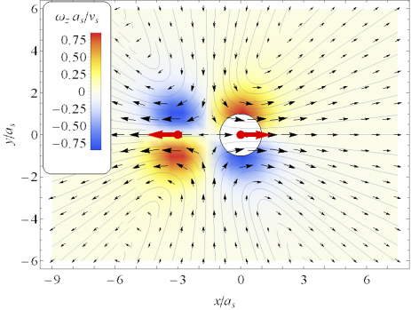
Figure 1: Schematic view of the 2-force model for a pusher type swimmer and its associated flow fields, as generated in WMCD. The swimmer’s body is indicated by the white disk, which moves in the positive $x$-direction as per the translational flow field (black arrows) at its centre. Red arrows indicate the position and direction of the swimming forces, while the coloured background shows the rotation field which is always into/out of the plane with negative/positive $\omega_{z}$ respectively. The full 3-dimensional flow field is symmetric under rotations about the $x$-axis. Field strengths are in arbitrary units.

The run and tumble motion exhibited by many micro-organisms, such as E. coli, is characterised by alternating phases of swimming and stopping, with increased rotational motion during the stopped ‘tumble’ phase. This has previously been modelled in simulations by instantaneous and random reorientations of swimmers at a Poisson distributed frequency Krishnamurthy and Subramanian (2015); Berg (1993).

In this work the tumble phase is stretched out over a finite time $t_{\mathrm{tumble}}$, during which there is an increased rotational diffusion and the swimming forces are turned off, so that the swimmer temporarily becomes a passive particle. To reduce the number of variables and make the data easier to decipher, we use fixed values of $t_{\mathrm{run}}$ and $t_{\mathrm{tumble}}$ rather than choosing them from a Poisson distribution. Hence each swimmer in the system cycles between running and tumbling with the same period $t_{\mathrm{run}}+t_{\mathrm{tumble}}$, although each is initialised at a different point in this cycle.

III.3 Simulation parameters

Table 1 lists the values of the physical parameters used for the results sections.

Table 1: System parameters in the results sections.

Parameter	Section IV	Sections V & VI
$L$	$\infty$	40 $\mu$m
$N_{s}$	1	64
$a_{s}$	1 $\mu$m	1 $\mu$m
$a_{p}$	0.5-2 $\mu$m	0.125-2 $\mu$m
$T$	0.3 mK	30-3000 K.
$v_{s}$	40 $\mu\mathrm{m}\,\mathrm{s}^{-1}$	40 $\mu\mathrm{m}\,\mathrm{s}^{-1}$
$\eta$	$0.85$ mPa s	$0.85$ mPa s
$\mathrm{Pe}_{\mathrm{rel}}$	$0.5$-$1\times 10^{8}$	2-1000
$t_{\mathrm{run}}$	$\infty$	1 s
$t_{\mathrm{tumble}}$	n/a	0.1 s
$\theta_{\mathrm{tumble}}$	n/a	$70^{\circ}$

Swimmer parameters are appropriate for E. coli Berg (1993), with only the run and tumble behaviour changing between sections. Where tumbling is present, the distance swum between tumbles compared to the swimmer radius is

$$\lambda=v_{s}t_{\mathrm{run}}/a_{s},$$ (17)

equalling 40 in our simulations. These runs dominate the time elapsed, so the active diffusion of the swimmers is well approximated by $D_{A}^{(s)}\approx a_{s}v_{s}\lambda/6$.

Because we have a finite $t_{\mathrm{tumble}}$ we need to specify how much swimmer orientations decorrelate when tumbling. This is done via Saragosti, Silberzan, and Buguin (2012)

$$\langle\hat{\textbf{v}}(t_{\mathrm{tumble}})\cdot\hat{\textbf{v}}(0)\rangle=\exp(-2D_{\mathrm{tumble}}^{RR}t_{\mathrm{tumble}}),$$ (18)

which will be useful for relating tumble angles to decorrelation times in Section V. In our simulations we used $\theta_{\mathrm{tumble}}=\arccos\langle\hat{\textbf{v}}(t_{\mathrm{tumble}})\cdot\hat{\textbf{v}}(0)\rangle=70^{\circ}$, inside the range of angles identified in Ref. 47. Reorientation from tumbling and normal rotational diffusion are comparable when averaged over the run and tumble cycle, with tumbling being dominant and sub-dominant at the lower and higher temperatures respectively in Sections V and VI. We note that the small size of E. coli is important here, and thermal rotations would be less significant were we modelling a larger microswimmer.

The swimmer volume fraction in Sections V & VI is $\phi_{s}=(4\pi/3)(a_{s}/L)^{3}N_{s}\approx 0.42\%$. The volume fraction of passive particles is unimportant because they do not influence each other’s motion, despite having correlated displacements. However, what is important for good statistics is the product of $N_{p}$ and total data collection time, which was a minimum of $1.85\times 10^{5}t_{\mathrm{run}}$ of effective single particle tracking time per data point.

IV Low noise particle trajectories

Our first results focus on interactions between individual swimmers and passive particles in the idealised scenario where swimmers move along an infinite straight path at constant speed. Such simulations have been done with more sophisticated techniques previously de Graaf and Stenhammar (2017); Shum and Yeomans (2017); Dunkel et al. (2010); Pushkin and Yeomans (2013); Pushkin, Shum, and Yeomans (2013), but are revisited here because they validate the use of WMCD for active systems while helping to visualise behaviour quantified in later sections.

Swimming along a perfectly straight path is not possible in WMCD, but a good approximation was achieved by switching off all rotations and reducing the temperature to raise the swimmer Péclet number to $1.3\times 10^{8}$. This also makes the Péclet number of relative motion high enough that thermal diffusion has negligible role in particle encounters.

In these simulations, performed in an infinite box, a single swimmer was set swimming in a straight line between $-40a_{s}\hat{\textbf{x}}$ and $+40a_{s}\hat{\textbf{x}}$. A single passive particle was placed an impact parameter $\rho$ off the swimmer’s path at $\textbf{r}_{p}(t=0)=\rho\hat{\textbf{y}}$, and its position was traced out as the swimmer passed by. The $x$-$y$ components of these trajectories are plotted in Fig. 2(a) for various $\rho$.

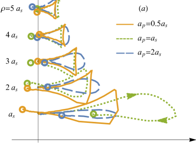
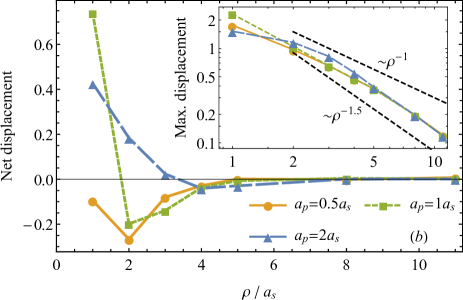
Figure 2: (a): Example trajectories of passive particles at different impact parameters with a swimmer on a straight path from left to right. All trajectories are travelled in a clockwise sense, as indicated on the $a_{p}=a_{s},\;\rho=a_{s}$ trajectory, starting on the vertical line and ending at the rings capping each trajectory. (b): Plots of the net displacement over the whole trajectory, and the maximum displacement in the $x$-direction (inset). All data were averaged over 100 trajectories to smooth out thermal fluctuations.

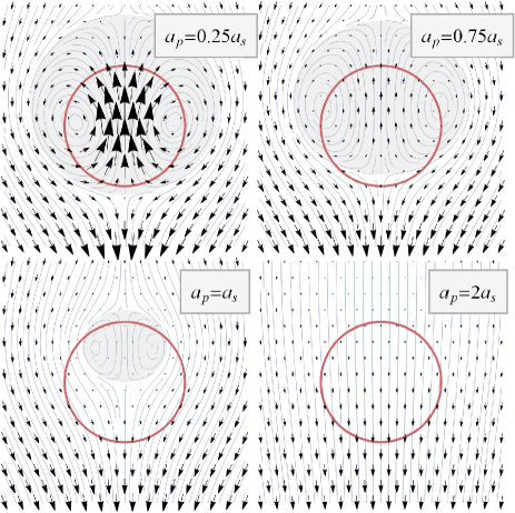
Figure 3: Translational flow fields relative to the swimmer velocity (upwards) as seen by particles of different sizes. Vector lengths across all plots have the same (arbitrary) units and can be compared directly. The disk, with radius $a_{s}$, indicates the swimmer size, and the flow field everywhere outside the plotted region is downwards.

Qualitatively, these trajectories match expectations by forming (almost) closed loops with cusps Dunkel et al. (2010) at large $\rho$, whilst at small $\rho$ the cusps become more rounded and the loops open up with a significant finite net displacement. The details of how the loops change at small $\rho$ are sensitive to the near-field details of the hydrodynamic mobility tensors and hence to passive particle radius $a_{p}$, as evidenced by the clear differences between the loops for $a_{p}=a_{s}$ and $2a_{s}$ at same $\rho$. To demonstrate this sensitivity to particle size, Fig. 3 shows the flow fields experienced by passive particles of different sizes, as seen in the swimmer’s reference frame. The most notable feature is the shaded recirculation zone (closed stream lines) close to the swimmer body that appears for small $a_{p}$, which the passive particles do not enter as the swimmer passes by. The $a_{p}=0.25a_{s}$ tile is very close to the flow-field that would be produced using the unmodified Oseen tensor, while the differences in the other 3 tiles arise due to the near-field corrections in the WMCD tensor. These corrections are therefore responsible for the differences in the trajectories in Fig. 2(a). This highlights the limitations of treating passive particles as infinitesimal tracers when near-field flows are important.

Fig. 2(b) provides a more quantitative description of the loops by plotting their size as measured by their maximal displacement parallel to the swimmer’s path. The unvarying loop shape at large $\rho$ means this choice is equivalent to the different measure used by Shum and Yeomans Shum and Yeomans (2017). Indeed, the decrease in loops size with a power law between $\rho^{-1}$ and $\rho^{-1.5}$ is consistent with their results.

It is the total net displacements of the passive particles that are key to their induced active diffusion, and these show a difference of sign and magnitude between large and small $\rho$. The large $\rho$ loops have negative net parallel displacement corresponding to a back-flow effect, and this can be estimated theoretically (see Appendix A and Ref. 49). The two key lengths here are $a_{p}$ and the distance between the centres of thrust and drag for our swimmer $A_{s}=3a_{s}$. When $\rho>a_{p},A_{s}$ we can work from the far field flow of a force dipole leading to the estimate that $\Delta(\rho)\sim-\rho^{-3}$.

The trajectories for smaller $\rho$ have positive net parallel displacements. For the limited but relevant range $a_{p}<\rho<A_{s}$ we obtain theoretically the much weaker dependence $\Delta(\rho)\sim+\rho^{-1}$ by treating the swimmer as two explicit point forces. In practice the crossover from positive to negative displacements can be seen in Fig. 2(a) to be sensitive to the values $a_{p}/a_{s}=0.5,1,2$ investigated, with larger $a_{p}$ changing sign at larger $\rho$, but then having a smaller net displacement: both effects are consistent with larger passive particles tracking a wider scale average of the advecting fluid flow.

So far we have only considered trajectories with a well defined net displacement in the reference frame of the background fluid. These correspond to moving along the open stream lines in Fig. 3. The trajectories of particles inside the shaded recirculation zone around the swimmer are instead well defined in the swimmer’s reference frame: they have zero net displacement in this frame. The passive particle is therefore displaced by $v_{s}t$ in the fluid frame, if trapped in the recirculation zone for time $t$. This behaviour is akin to entrainment observed in real systems Jeanneret et al. (2016); Mathijssen, Jeanneret, and Polin (2018), albeit driven by internal flows rather than steric repulsion and a non-slip boundary at the swimmer surface. We therefore describe such trajectories as ‘entrained’ in the following sections.

V Velocity Autocorrelations

Next we discuss the velocity autocorrelation of passive particles in active systems. The systems are now made periodic with cubic box, we use a reference temperature $T_{0}$ representative of 300K, and swimmers are free to rotate by rotational diffusion, hydrodynamic interactions and tumbling. Note that in these simulations we confirmed $D_{A}$ is proportional to swimmer concentration, as demonstrated in Fig. 4 whose results are discussed in detail in Section VI, so we are in the dilute limit where swimmer-swimmer interactions can be neglected. We also note that we find $D_{A}$ to vary roughly as $(a_{p}/a_{s})^{0.2}$ at small $a_{p}$. This power cannot be explained by considering any one mechanism, and is a sign that we are in a complex regime with many contributing factors. $D_{A}$ itself has integrated out too much information to unpick these factors, motivating our focus on velocity autocorrelations instead.

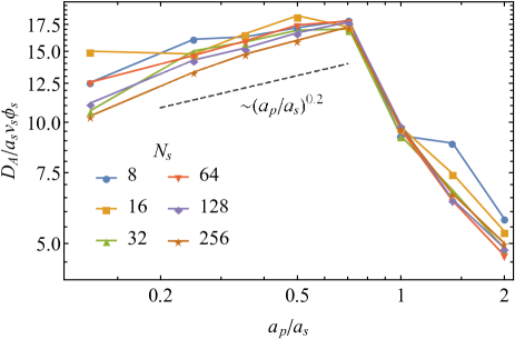
Figure 4: Plots of active diffusion of passive particles of different sizes, in systems with different swimmer volume fractions, $\phi_{s}\propto N_{s}$. The vertical axis is scaled by $\phi_{s}$, leading to the collapse of the data sets, thereby confirming $D_{A}\propto\phi_{s}$. The dashed line gives a rough guide to the weak power law behaviour seen on the small $a_{p}/a_{s}$ side of the data.

We begin with a qualitative discussion of these and will use this as the basis for a quantitative discussion in Section V.1. We will denote passive particle and swimmer autocorrelations with $C_{vv}^{(p)}$ and $C_{vv}^{(s)}$ respectively. Fig. 5(a) shows the three forms of $C_{vv}^{(p)}$ we find in our data, alongside an example $C_{vv}^{(s)}$ which is a simple exponential decay with some fine details coming from run and tumble motion which we will ignore.

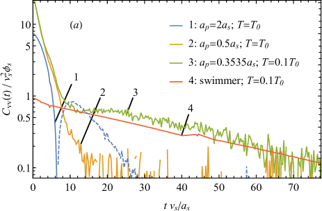
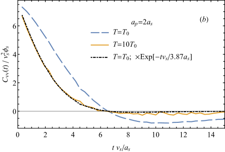
Figure 5: Example velocity autocorrelations exhibiting the distinct forms observed across all data collected. (a): data shown on a linear-log scale, with passive particle sizes and temperatures as indicated on the legend. The swimmer data (4) includes a factor of $\phi_{s}$ relative to the passive particle data (1-3) so that it starts at $C_{vv}(0)/v_{s}^{2}\approx 1$. The dashed line is a continuation of curve 1 with a negative sign to see it on the log scale. (b): re-plots curve 1 with a linear vertical scale alongside data for the same $a_{p}$ at a higher temperature. The dot-dashed line demonstrates there is an exponential decay factor between the two curves.

In curve 1, which is typical of systems with $a_{p}\geqslant a_{s}$, we see negative tails compatible with the forwards-backwards movement in the loop trajectories discussed in the preceding section. In curve 2, with smaller $a_{p}$ at the same temperature, this negative tail appears to have vanished, or at least been reduced to the size of noise in our data.

Note the value of $C_{vv}^{(p)}(0)$ has increased between these curves, which is due to small particles having a larger response to the swimming forces in the near-field. The size of the increase, at more than a factor of 2, is indicative of how much the near-field contributes to $C_{vv}^{(p)}(0)$, and we anticipate a similar rise in $D_{A}$. Importantly, however, $C_{vv}^{(p)}(0)$ reaches a maximum at around $a_{p}=0.5a_{s}$, below which it is essentially constant. This will be discussed in greater detail in Section V.1.2.

Finally, curve 3 in Fig. 5(a) shows that the reduction of temperature reveals a long-time exponential tail. This tail is present in the all our $T=0.1T_{0}$ data with $a_{p}\leqslant a_{s}/\sqrt{2}$, although its amplitude is not always the same. This tail runs almost parallel to $C_{vv}^{(s)}$ in curve 4, suggesting the passive particles are tracking the swimmer motion, that is they are entrained. This is further supported by the quantitative similarity between $C_{vv}^{(p)}(t)$ and $\phi_{s}C_{vv}^{(s)}(t)$, which is expected if a fraction of order $\phi_{s}$ of passive particles are entrained at any one time. This entrainment is both initiated and ended by crossing the boundary of the closed stream lines.

There is in fact a subtle but important difference in the gradients of curves 3 and 4 at large times. First, tracing the long-time exponential back to $t=0$ leads to a value larger than $\phi_{s}C_{vv}^{(s)}(0)$, fitting with the entrainment volume around a swimmer being larger than the swimmer’s own volume, as per Fig. 3. Second, this means the mid-time section of the curve undershoots the long-time exponential, which is consistent with there being a negative contribution akin to that seen in curve 1. This too is expected as the loop trajectories should still be present, and indeed the location of the peak of the negative (dashed) section of curve 1 coincides with the depression in curve 3. We believe this story applies to curve 2 as well, but in this case the negative contribution is closely matched to the positive tail so they cancel each other out.

Our final comment on the qualitative features of $C_{vv}^{(p)}$ is that we find curves at different temperatures but the same particle size can be successfully mapped onto each other by introducing an exponential decay factor between them. This is demonstrated in Fig. 5(b), and will be central to our approach going forwards.

V.1 Ansatz function

We now attempt to quantify the velocity autocorrelations, starting with the swimmers since they have the simplest form, and we have seen that the passive particles can pick up the same form.

Ignoring some fine details seen in Fig. 5(a) that arise due to the fixed times in the run and tumble cycle, it is clear we have a simple exponential decay of the form,

$$C_{vv}^{(s)}(t)=v_{s}^{2}\frac{t_{\mathrm{run}}}{t_{\mathrm{run}}+t_{\mathrm{tumble}}}e^{-t/\tau_{s}}$$ (19)

where the run and tumble factors account for the time spent not swimming and hence why the swimmer curve begins just below 1. The exponential decay comes only from reorientations because translational diffusion does not change the swimming direction, and therefore does not affect $C_{vv}^{(s)}$ beyond the Brownian spike at $t=0$, which we are ignoring. Hence we have

$$\tau_{s}^{-1}=\tau_{\mathrm{r\&t}}^{-1}+\tau_{\mathrm{rot}}^{-1}$$ (20)

where the decay time associated with normal rotational diffusion is

$$\tau_{\mathrm{rot}}=\left(2D_{s}^{RR}\right)^{-1}=(2/3)\mathrm{Pe}_{s}a_{s}/v_{s}$$ (21)

and the decay time for run and tumble motion, spread across the whole run and tumble cycle, is

$$\tau_{\mathrm{r\&t}}=\left(2D_{\mathrm{tum}}^{RR}\frac{t_{\mathrm{tumble}}}{t_{\mathrm{run}}+t_{\mathrm{tumble}}}\right)^{-1}=1.02t_{\mathrm{run}}.$$ (22)

Note the final expression uses Eq. (18) and our typical tumble angle of $70^{\circ}$. Together, these predict $\tau_{s}v_{s}/a_{s}=39.2$, in good agreement with the decay time observed in curve 4 in Fig. 5(a).

We also expect the $C_{vv}^{(p)}$ to decay with $\tau_{s}$. In the entrainment tail the reasoning is the same as for the swimmers - the decorrelation of the direction of $\textbf{v}(t)$ - but we also expect it to play a role in decorrelating non-entrained loops where swimmer rotations effectively force the passive particles onto different stream lines, as well as rotating the flow field. By similar reasoning, we expect an additional decorrelation time coming from (translational) Brownian motion, $\tau_{B}$. This should also feature in the entrainment tail where it drives entry and escape of the entrained volume. In higher density systems we might expect a similar term for swimmer-swimmer interactions, but we do not consider those here.

We express the total $C_{vv}^{(p)}$ as the sum of terms from entrainment and non-entrained loops:

$$C_{vv}^{(p)}(t)=C_{vv}^{(\mathrm{Ent})}(t)+C_{vv}^{(\mathrm{Loop})}(t)$$ (23)

which we now detail separately.

V.1.1 The entrainment term

Entrained particles follow swimmers, therefore we expect $C_{vv}^{(\mathrm{Ent})}$ to be given by Eq. (19) modified to account for Brownian escape and the actual entrained volume fraction $\phi_{\mathrm{Ent}}$. This implies that

$$C_{vv}^{(\mathrm{Ent})}(t)=\phi_{\mathrm{Ent}}C_{vv}^{(s)}(t)\,\exp\left(-\sqrt{t/\tau_{B,\mathrm{Ent}}}\right).$$ (24)

The details of the decorrelation factor, including the perhaps unexpected square root, will be discussed after $\phi_{\mathrm{Ent}}$.

As Fig. 3 showed, $\phi_{\mathrm{Ent}}$ varies with particle size, and has 3 regimes of behaviour. For $a_{p}>a_{s}$, there is no entrainment as the response to the swimming forces is always less than that of the swimmer. For $a_{p}\ll a_{s}$ the entrainment volume is constant and is approximately 4 times the swimmer volume for our model. As $a_{p}$ increases the volume begins to decrease when the hydrodynamic near-field of the particle, i.e the distance within which the hydrodynamic response is different to the Oseen tensor, is comparable to the geometric size of the swimmer, $A_{s}$. In our WMCD simulations that hydrodynamic range is $5.35a_{p}$, leading us to define the ratio

$$\mathcal{R}=\frac{5.35a_{p}}{A_{s}}=1.78\frac{a_{p}}{a_{s}}$$ (25)

with which we would anticipate the regime change at $\mathcal{R}\approx 1$. Assuming a simple linear interpolation between the large and small $a_{p}$ regimes, we have

$$\phi_{\mathrm{Ent}}\approx\phi_{s}\left\{\begin{array}[]{ll}4&\mathcal{R}<1\\ 0&a_{p}>a_{s}\\ 9.12-5.12\mathcal{R}&\mathrm{between}\end{array}\right..$$ (29)

We now address the Brownian decorrelation factor. This can be estimated by the fraction of particles left inside a stagnant, entrained sphere after diffusing for time $t$ if we assume an initially uniform distribution and that they are swept away, without return, upon first passage across the boundary of the entrained volume. This calculation is the same as the one leading to Eq. (6.19) in Ref. 50, which decays approximately as $\exp[-\sqrt{t}]$ at small times. It is the asymmetry in this first passage problem that leads to the square root rather than the simple exponential decay used in other decay factors.

That calculation gives us a handle on the form of the decay time $\tau_{B,\mathrm{Ent}}\sim a_{s}^{2}/D_{\mathrm{rel}}=(a_{s}/v_{s})\mathrm{Pe}_{\mathrm{rel}}$. Using all the other parameters in $C_{vv}^{(\mathrm{Ent})}$ as described above, we set the numerical prefactor to match the entrainment tail in Fig. 5(a) curve 3. This gives us

$$\tau_{B,\mathrm{Ent}}\approx 0.07\mathrm{Pe}_{\mathrm{rel}}a_{s}/v_{s},$$ (30)

corresponding to diffusing a distance of $\sqrt{6D_{\mathrm{rel}}\tau_{B,\mathrm{Ent}}}\approx 0.65a_{s}$, which is reassuringly less than $a_{s}$.

V.1.2 The loop term

The non-entrained loop contribution in Eq. (23) needs to provide the negative tail seen in the $a_{p}=2a_{s}$ data in Fig. 5. The functional form of this could in principle be calculated in the far-field where the loop trajectory is known mathematically for a dipole swimmer Dunkel et al. (2010), but the near-field is not entirely absent in our expression so we would expect model-dependent terms to enter. We therefore choose to take a simpler route and use a functional form that has the correct features:

$$C_{vv}^{(\mathrm{Loop})}(t)=c_{0}(1-c_{2}(t/\tau_{L})^{2})\\ \times\exp\left[-\left(\tau_{L}^{-1}+\tau_{s}^{-1}+\tau_{B,\mathrm{Loop}}^{-1}\right)t\right].$$ (31)

The task is now to identify all the new parameters, starting with the coefficients $c_{0}$ and $c_{2}$.

$c_{2}$ will not be explored in detail, but we note it must satisfy $0<c_{2}\leqslant 1/2$ to ensure both a negative tail exists and $C_{vv}^{(\mathrm{Loop})}$ has a positive integral. In Section VI we will use two values to show its effect on $D_{A}$.

$c_{0}$ sets the value at $t=0$ and can be written as

$$c_{0}=C_{vv}^{(p)}(0)-\phi_{\mathrm{Ent}}C_{vv}^{(s)}(0).$$ (32)

The total $C_{vv}^{(p)}(0)$ is most easy to access in our data by interpolating small $t$ values back to 0 assuming a simple exponential decay, thereby avoiding the Brownian spike which overwhelms the zero-time data. Values obtained by this procedure are shown in Fig. 6(a), where we see 2 distinct regimes: $C_{vv}^{(p)}$ is flat at small $a_{p}/a_{s}$ and decays at larger values.

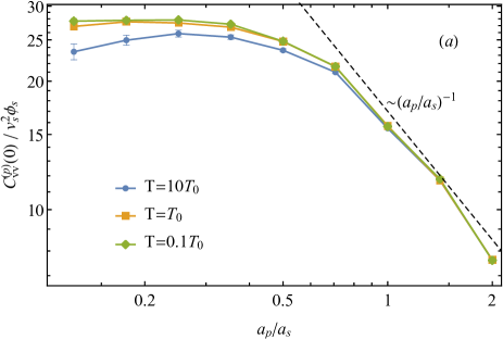
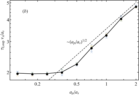
Figure 6: (a): Plot of $C_{vv}^{(p)}(0)$ against $a_{p}$ for our 3 different temperatures. (b): Plot of the ansatz parameter $\tau_{L}$ against $a_{p}$, with each marker showing the mean of the values for the 3 temperatures, whose individual values are marked with crosses at low opacity. The dashed guidelines in both plots are only to indicate the rough behaviour.

The flat regime is simply the result of passive particles being small compared to the distance between the swimming forces, $A_{s}$, so they act like infinitesimal tracer particles. Indeed, the regime change occurs close to $\mathcal{R}=1\Leftrightarrow a_{p}/a_{s}=0.56$, supporting this picture. What is less easy to understand is the apparent dependence on temperature in this regime, with the high temperature data being too small to be accounted for by our error margins. We attribute this apparent $T$-dependence to the assumption of a simple exponential decay when interpolating back, which underestimates the contribution from $\exp[-\sqrt{t/\tau_{B,\mathrm{Ent}}}]$. The corresponding error is largest at small $\mathrm{Pe}_{\mathrm{rel}}$ and only when the entrainment term is present, both fitting with where the difference occurs in Fig. 6(a).

The decay at larger $a_{p}/a_{s}$ can be understood using scaling arguments, detailed in Appendix B, which use the fact our mobility tensor can be written as $a_{p}^{-1}\bm{\mathcal{G}}(\textbf{r}/a_{p})$ when $a_{p}\gg A_{s}$, leading to $c_{0}\sim a_{p}^{-1}$. We can capture both regimes with the piecewise function

$$c_{0}\approx 24v_{s}^{2}\phi_{s}\left\{\begin{array}[]{ll}1&\mathcal{R}<1\\ \mathcal{R}^{-1}&\mathcal{R}\geqslant 1\end{array}\right.,$$ (35)

where the front factor is read straight from our data, accounting for the known entrainment contribution.

We now turn our attention to the as yet undetermined time scales $\tau_{L}$ and $\tau_{B,\mathrm{Loop}}$. $\tau_{L}$ is a representative time scale for the loop trajectories, which comes from an average over impact parameters. We do not know its dependence on $a_{p}$, but we do know it is independent of temperature, as confirmed by Fig. 5(b) where the data at different temperature change sign at the same time. Appendix C describes how to use this fact to isolate $\tau_{B,\mathrm{Loop}}$ in measurements of initial decay rates knowing only $\tau_{\mathrm{rot}}$. This approach finds

$$\tau_{B,\mathrm{Loop}}\approx 1.73\mathrm{Pe}_{\mathrm{rel}}a_{s}/v_{s},$$ (36)

proportional to $\mathrm{Pe}_{\mathrm{rel}}$ as expected, and associated with diffusion over a distance close to $A_{s}$.

Before progressing, we note that this decorrelation appears as a simple exponential because Brownian motion outside the entrained volume lacks the asymmetry that provided the square root in the analogous factor in the entrainment term.

Finally, we can feed $\tau_{B,\mathrm{Loop}}$ back into our fitted initial decay rates and solve for $\tau_{L}$. This leads to Fig. 6(b), where, similarly to $C_{vv}^{(p)}(0)$, we find it to be constant below $\mathcal{R}\lesssim 1$, while it rises with an apparent power law $\sim a_{p}^{1/2}$ above.

While the small $\mathcal{R}$ behaviour has the usual explanation that the passive particles are behaving as infinitesimal tracers, the apparent power law is harder to understand as it disagrees with the scaling argument in Appendix B, which predicts $\tau_{L}\sim a_{p}^{1}$. This discrepancy could come from the periodicity of our system, which was not accounted for in our calculations, or could simply be a sign our data does not extend to large enough $a_{p}$ to see the expected behaviour. For the purposes of this work it is sufficient to write down the empirical form as

$$\tau_{L}\approx 2\frac{a_{s}}{v_{s}}\left\{\begin{array}[]{ll}1&\mathcal{R}<1\\ \mathcal{R}^{1/2}&\mathcal{R}\geqslant 1\end{array}\right..$$ (39)

With this, our ansatz form for $C_{vv}^{(p)}(t)$ is fully defined up to the single remaining free parameter $c_{2}$.

VI Active diffusion

We now move from the velocity autocorrelation to the active diffusivity, obtained by integrating $C_{vv}^{(p)}$ as per Eq. (4). This we show for both numerical integration of the simulation data and analytical integration of our ansatz $C_{vv}^{(p)}$ using the approximate expressions for parameters in the previous section. These are shown in Fig. 7.

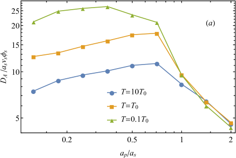
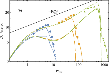
Figure 7: (a): active diffusivity calculated from simulation data, plotted against particle size. Data points are joined here to highlight the non-monotonic behaviour. Note the $T=T_{0}$ data is the same as the $N_{s}=64$ data in Fig. 4. (b): the same data plotted against $\mathrm{Pe}_{\mathrm{rel}}$ and accompanied by plots of $D_{A}$ calculated with our ansatz function using $c_{2}=0.22$ (short dashes) and $c_{2}=0.5$ (long dashes). The solid line above the data is included to indicate the apparent power law we find across our $a_{p}\leqslant a_{s}/\sqrt{2}$ data.

Beginning with our data plotted against $a_{p}/a_{s}$ in Fig. 7(a), we observe two main features: non-monotonicity with a turning point just below $a_{p}/a_{s}=1$; and a temperature-dependence on the small $a_{p}$ side. The non-monotonicity requires different physics to be dominating at different regimes. Using the understanding from previous sections, the presence and absence of entrainment at small and large $a_{p}$ respectively accounts for this behaviour, and is supported by the turning point being close to $\mathcal{R}=1$.

The quantitative behaviour in the two regimes can also be understood using our analysis of $C_{vv}^{(p)}$. The decay on the large $a_{p}$ side comes primarily from the decay of $C_{vv}^{(p)}(0)$, which is not fully compensated for by the increase in $\tau_{L}$, at least not over the range of our data. Note that $\tau_{L}\ll\tau_{\mathrm{r\&t}}\ll\tau_{\mathrm{rot}},\tau_{B,\mathrm{Loop}}$ in the $T=0.1T_{0}$ data here, meaning the attenuation of the negative tail in $C_{vv}^{(p)}(t)$ is dominated by $\tau_{L}$, allowing us to neglect the other decorrelation times in this regime.

Work by Pushkin and YeomansPushkin and Yeomans (2013) has argued that the contribution from far field loops truncated by run and tumble events leads to a constant value of $D_{A}$ independent of the run length. We expect our additional decorrelation mechanisms to fall under the same formalism, and hence would expect a constant term in $D_{A}$ that might be seen if we extended our range of $a_{p}/a_{s}$. However, feeding our parameters into their calculation would put the value of this constant at $D_{A}/a_{s}v_{s}\phi_{s}=20.25$, which is clearly missing or greatly reduced in our data. We believe our periodic boundaries are the cause of its absence since it is an effect dominated by flow fields at impact parameters of order the run length. In our case, the run length equals the side length of our box, so there will be significant interference from the swimmer’s periodic images.

Our final comment on the large $a_{p}$ regime is that the collapse of the curves at different temperatures here is misleading. As Fig. 5(b) showed, there is a significant difference in $C_{vv}^{(p)}$ here and the dynamics truly are affected by the temperature. We believe our $10T_{0}$ data happened to have an equal loss of the negative tail and initial positive decay, but this is not generally true and we expect an intermediate temperature, e.g. $5T_{0}$, would have a higher $D_{A}$ here because it’s negative tail will have been affected the most by the decorrelations. By the same reasoning, a temperature larger than $10T_{0}$ would have smaller $D_{A}$ because there is very little of the negative tail left to lose, leading to a greater loss from the positive part.

The variation at small $a_{p}$ is driven primarily by diffusive processes, so our $C_{vv}^{(p)}$ analysis predicts this behaviour to be a function of $\tau_{\mathrm{rot}}\sim\mathrm{Pe}_{s}\sim T_{0}/T$ and $\tau_{B,\mathrm{Ent}},\tau_{B,\mathrm{Loop}}\sim\mathrm{Pe}_{\mathrm{rel}}$, instead of a function of $a_{p}/a_{s}$. In practice we find $\tau_{\mathrm{rot}}$ is large enough that it has a negligible influence, leading to our data falling onto a master curve when plotted against $\mathrm{Pe}_{\mathrm{rel}}$, as shown in Fig. 7(b). The apparent power law we observe across our data is close to $\mathrm{Pe}_{\mathrm{rel}}^{0.2}$, not $\mathrm{Pe}_{\mathrm{rel}}^{1}$ or $\mathrm{Pe}_{\mathrm{rel}}^{1/2}$ as we might have expected from the form of the two Brownian decorrelation factors.

Our ansatz function provides and explanation for this, although we must first specify a value of $c_{2}$. The first value we use in Fig. 7(b) is $c_{2}=0.22$, which was chosen by a least squares fit of the ansatz to the data, setting all other parameters as described in Section V.1. Here we see good agreement with the data at all temperatures, including the appearance of a shallow apparent power law. Extending the plot down to smaller $\mathrm{Pe}_{\mathrm{rel}}$ finds the expected $\mathrm{Pe}_{\mathrm{rel}}^{1}$ behaviour does appear eventually. Importantly, the ansatz plots have undulations, which are made extreme when using the largest allowed value of $c_{2}=0.5$. This results from the two terms in the ansatz, with the loop term providing the peak at small $\mathrm{Pe}_{\mathrm{rel}}$ and the entrainment providing the second rise. These undulations are more subtle in our simulation data, but they are still visible in the curvatures of the $10T_{0}$ and $1T_{0}$ data. Hence we attribute the small power law to a transitional regime between loop and entrainment dominance.

It is useful here to compare to Kasyap, Koch and Wu’s calculation of $D_{A}\sim\mathrm{Pe}^{1/2}$ for small $\mathrm{Pe}$ in a slender-body swimmer model Kasyap, Koch, and Wu (2014). In contrast, both terms in our anstaz lead to $D_{A}\sim\mathrm{Pe}^{1}$ in this limit. We suspect the origin of this discrepancy might lie in their result assuming the distance swum in a single run is much smaller than the typical displacement by Brownian motion in the same time, whereas the reverse was true for all systems we used to construct our ansatz.

Finally, we note that the properties of our swimmers, especially the lack of steric interactions, will limit the applicability of our understanding to experimental systems. Our nono-monotonicity is nevertheless in qualitative agreement with the experiments of Patteson et al. Patteson et al. (2016) This encourages us to propose that the cause is to be found in the transition between a regime dominated by entrainment events for small passive particles, and one for larger particles where far field loops are most important. We believe that this prediction could be testable with the experimental trajectories already available from the experiments in Ref. 33.

VII Conclusions

We have looked at the effect of both particle size and temperature on the active diffusion of spherical passive particles in 3D periodic systems of microswimmers. For this we used a ‘smart’ version of the Wavelet Monte Carlo dynamics algorithm to simulate active systems with hydrodynamically correlated rotations and translations, biased by swimming force. This gave us an efficient algorithm that includes correlated thermally-driven Brownian motion that is sensitive to particle size.

Our first results were geared towards validating active, non-thermal behaviour in smart WMCD, for which we simulated the trajectories of single passive particles at varying impact parameters from a passing swimmer at very large Péclet number. These results were consistent with previous work, demonstrating the expected cusped-loop trajectories at large impact parameter, whose net and maximum displacements decayed with the expected power laws.

We then turned our attention to dilute mixtures of swimmers and passive particles with thermal fluctuations present. By using a range of temperatures and passive particle sizes we were able to identify the physics driving active diffusion via the behaviour of the velocity autocorrelation. Analysis of this led to constructing an ansatz function to unify the diverse forms of $C_{vv}^{(p)}$ observed. This function was expressed as the sum of contributions from entrainment and non-entrained loop trajectories, both subject to exponential decorrelation factors coming from swimmer rotations and Brownian motion. More generally, any mechanism causing passive particles to cross swimmer-induced stream lines could be included in this way.

Most parameters in our ansatz fall under one of two categories: decorrelation times that vary with the appropriate Péclet number; and parameters describing the $\mathrm{Pe}\rightarrow\infty$ limit governed by the comparison between the hydrodynamic response of the passive particle and the geometric size of the swimmer. By itself, the second category of parameters leads to $D_{A}$ having two regimes when plotted against $a_{p}$, with a decay away from the flat, small-$a_{p}$ regime where particles act as infinitesimal tracers. The decorrelation factors then introduce a gradient to the small-$a_{p}$ regime, leading to non-monotonic behaviour.

Plotting $D_{A}$ against $\mathrm{Pe}_{\mathrm{rel}}$ reveals a master curve for the small $a_{p}$ regime. The behaviour of this master curve over the range of Péclet numbers studied is made complicated by the entrainment and loop contributions appearing and plateauing at different values, with their sum leading to a weak apparent power law.

Finally, we note that the simplicity of our swimmer model means it is not expected to give quantitatively relevant results for comparison with experiment. Instead, the strength of our results lies in the identification of the role of particle size and Péclet number(s) in the velocity autocorrelation. In the process we highlighted the importance of temperature and near-field effects, both of which are often neglected in theoretical and computational studies of similar systems.

Data Availability

The data that support the findings of this study are available from the corresponding author upon reasonable request.

Appendix A Loop size calculations

We first consider the noise-free transits as graphed in Fig. 2. The displacement of a passive particle $\bm{\Delta}(t)$ due to the passage of a swimmer incident with impact parameter $\rho$ and swimmer velocity $v_{s}\hat{\mathbf{z}}$ obeys

$$d\bm{\Delta}/dt=\mathbf{v}(\bm{\Delta}+\rho\hat{\bm{\rho}}-v_{s}t\hat{\mathbf{z}}),$$ (40)

where $\mathbf{v}(\mathbf{r})$ is the flow field established by the swimmer and $\hat{\bm{\rho}}$ is the radial unit vector in cylindrical polar coordinates.

As constructed, the swimmer approaches from below so that $\Delta_{z}-z_{s}$ decreases from $+\infty$, down to $-\infty$ for an orbit which does not get entrained. It is then convenient to write $\mathbf{v}(\mathbf{r})=v_{s}\mathbf{g}(\rho\hat{\bm{\rho}},z-z_{s})$ and $v_{s}dt=dz_{s}$ so $z_{s}$ is the vertical rise of the swimmer, which leads to

$$\bm{\Delta}=\int\limits_{-\infty}^{z_{s}}\mathbf{g}(\rho\hat{\bm{\rho}}+\bm{\Delta}_{\rho},\Delta_{z}-z_{s}^{\prime})dz_{s}^{\prime}.$$ (41)

For the unentrained trajectories we can follow earlier work Pushkin, Shum, and Yeomans (2013) in expanding this for the total deflection as a series in $\mathbf{g}$ . It is convenient then to parameterise in terms of $z=-z_{s}$ which is to zero’th order the height of the passive above the swimmer, giving

$$\bm{\Delta}=\int\limits_{z}^{\infty}\mathbf{g}(\rho\hat{\bm{\rho}}+\bm{\Delta}_{\rho},\Delta_{z}+z^{\prime})dz^{\prime}.$$ (42)

Expanding $\bm{\Delta}$ in implied powers of $\mathbf{g}$ then gives $\bm{\Delta}=\bm{\Delta}^{(1)}+\bm{\Delta}^{(2)}+O(\mathbf{g}^{3})$ where

$$\bm{\Delta}^{(1)}(\rho\hat{\bm{\rho}},z)=\int\limits_{z}^{\infty}\mathbf{g}(\rho\hat{\bm{\rho}},z^{\prime})dz^{\prime}$$ (43)

and

$$\bm{\Delta}^{(2)}(\rho\hat{\bm{\rho}},z)=\int\limits_{z}^{\infty}\bm{\Delta}^{(1)}(z^{\prime})\cdot\mathbf{\nabla}\mathbf{g}(\rho\hat{\bm{\rho}},z^{\prime})dz^{\prime}.$$ (44)

On the LHS $\rho$ and $z$ parameterise the transit in terms of impact parameter and time (as $-z/v_{s}$) through it. However on the RHS they are simply cylindrical polar coordinates of the flow around the swimmer.

We now focus on swimmers with azimuthal symmetry, so we write

$$\bm{\Delta}^{(1)}(\rho\hat{\bm{\rho}},z)=\mathbf{h}(\rho,z),$$ (45)

which can be thought of as a divergence free flow field. Moreover, in the far field the swimmer flow is proportional to that of a force dipole $-\partial(\bm{\mathcal{G}}^{\mathrm{TT}}_{\mathrm{O}}\cdot\hat{\textbf{z}})/\partial z$ so we infer that in the far field $\mathbf{h}$ approaches $\bm{\mathcal{G}}^{\mathrm{TT}}_{\mathrm{O}}\cdot\hat{\textbf{z}}$, where $\bm{\mathcal{G}}^{\mathrm{TT}}_{\mathrm{O}}$ is the Oseen tensor. It then follows that for any force free swimmer the first order advective deflections of a point passive particle form a closed loop ending up with $\bm{\Delta}^{(1)}(\rho,-\infty)=0$.

At second order we now need

$$\bm{\Delta}^{(2)}(\rho,z)=\int\limits_{z}^{\infty}\mathbf{h}(\rho,z^{\prime})\cdot\mathbf{\nabla}\left(-\frac{\partial}{\partial z^{\prime}}\mathbf{h}(\rho,z^{\prime})\right)dz^{\prime}.$$ (46)

As $\mathbf{h}$ is divergence free we can rewrite the integrand as $\mathbf{\nabla}\cdot\left[\mathbf{h}(\rho,z^{\prime})\left(-\frac{\partial}{\partial z^{\prime}}\mathbf{h}(\rho,z^{\prime})\right)\right]$ leading to

$$\bm{\Delta}^{(2)}(\rho,z)=h_{z}(\rho,z)\frac{\partial}{\partial z}\mathbf{h}(\rho,z)\\ -\frac{1}{\rho}\frac{\partial}{\partial\rho}\rho\int\limits_{z}^{\infty}h_{\rho}(\rho,z^{\prime})\frac{\partial}{\partial z^{\prime}}\mathbf{h}(\rho,z^{\prime})dz^{\prime}.$$ (47)

For the transverse displacement we can now give a full result

$$\Delta^{(2)}_{\rho}(\rho,z)=h_{z}(\rho,z)\frac{\partial}{\partial z}h_{\rho}(\rho,z)+\frac{1}{2\rho}\frac{\partial}{\partial\rho}\rho\,h_{\rho}(\rho,z)^{2},$$ (48)

and note that this gives zero for the complete transit.

The longitudinal displacement is given by

$$\Delta^{(2)}_{z}(\rho,z)=h_{z}(\rho,z)\frac{\partial}{\partial z}h_{z}(\rho,z)\\ -\frac{1}{\rho}\frac{\partial}{\partial\rho}\rho\int\limits_{z}^{\infty}h_{\rho}(\rho,z^{\prime})\frac{\partial}{\partial z^{\prime}}h_{z}(\rho,z^{\prime})dz^{\prime}.$$ (49)

The integrand here can be expressed using the divergence free property of $\mathbf{h}$ as

$$h_{\rho}(\rho,z^{\prime})\left(-\frac{1}{\rho}\frac{\partial}{\partial\rho}\rho h_{\rho}(\rho,z^{\prime})\right)=-\left(\frac{1}{\rho}+\frac{1}{2}\frac{\partial}{\partial\rho}\right)h_{\rho}(\rho,z^{\prime})^{2}.$$ (50)

This then gives the deflection through a full transit as

$$\Delta^{(2)}_{z}(\rho,-\infty)=\frac{1}{\rho^{2}}\rho\frac{\partial}{\partial\rho}\left(1+\frac{1}{2}\rho\frac{\partial}{\partial\rho}\right)\int\limits_{-\infty}^{\infty}h_{\rho}(\rho,z^{\prime})^{2}dz^{\prime}.$$ (51)

In the far field force dipole limit $\mathbf{h}$ is just given by the Oseen tensor and we have $\int_{-\infty}^{\infty}h_{\rho}(\rho,z^{\prime})^{2}dz^{\prime}\propto+1/\rho$ and hence $\Delta_{z}^{(2)}\propto-1/\rho^{3}$, where the negative sign signifies dominance by back-flow around the swimmer. For a swimmer modelled as two opposed point forces separated by $A_{s}$ and with dipole strength $\kappa=A_{s}F_{s}$, near approaches $\rho\ll A_{s}$ lead to $\int_{-\infty}^{\infty}h_{\rho}(\rho,z^{\prime})^{2}dz^{\prime}\propto+\rho/A_{s}^{2}$ and hence $\Delta_{z}^{(2)}\propto+1/(\rho A_{s}^{2})$, this time with a positive sign.

The full forms for a swimmer modelled by two point forces separated by $A_{s}$ can be found as follows. The transverse component of the Oseen tensor is given by $(\rho z/8\pi\eta)(\rho^{2}+z^{2})^{-3/2}$ and integrating this with respect to $z$ gives $-(\rho/8\pi\eta)(\rho^{2}+z^{2})^{-1/2}$, which then leads to

$$h_{\rho}(\rho,z)=\frac{\kappa}{8\pi\eta A_{s}}\left[(1+(\zeta-\alpha)^{2})^{-1/2}\right.\\ -\left.(1+(\zeta+\alpha)^{2})^{-1/2}\right]$$ (52)

where $\zeta=z/\rho$ and $\alpha=A_{s}/2\rho$. In the limit of large $\alpha$ the integral over $h_{\rho}(\rho,z^{\prime})^{2}$ is then dominated by two well separated Lorentzians each of width $\rho$ and height $\propto A_{s}^{-2}$, leading to $\int_{-\infty}^{\infty}h_{\rho}(\rho,z^{\prime})^{2}dz^{\prime}\propto\rho/A_{s}^{2}$ as used in the paragraph above.

To get the full result we write

$$\int\limits_{-\infty}^{\infty}h_{\rho}(\rho,z^{\prime})^{2}dz^{\prime}=\frac{\rho\kappa^{2}}{(8\pi\eta A_{s})^{2}}[I(0)-2I(\alpha)+I(0)],$$ (53)

where

$$I(\alpha) =\int\limits_{-\infty}^{\infty}\left(1+(\zeta-\alpha)^{2}\right)^{-1/2}\left(1+(\zeta+\alpha)^{2}\right)^{-1/2}d\zeta$$ (54)

$$=\frac{1}{\pi}\int\limits_{-\infty}^{\infty}\int\limits_{-\infty}^{\infty}\int\limits_{-\infty}^{\infty}d\zeta\,d\lambda\,d\mu\Big{[}\exp\left(-\lambda^{2}(1+(\zeta-\alpha)^{2})\right)$$

$$\hphantom{somemorespace}\times\exp\left(-\mu^{2}(1+(\zeta+\alpha)^{2})\right)\Big{]}$$

$$=\frac{1}{\sqrt{\pi}}\int\limits_{-\infty}^{\infty}\int\limits_{-\infty}^{\infty}d\lambda\,d\mu\,\Bigg{[}(\lambda^{2}+\mu^{2})^{-1/2}$$

$$\hphantom{somespace}\times\exp\left(-(\lambda^{2}+\mu^{2})-\frac{4\alpha^{2}\lambda^{2}\mu^{2}}{\lambda^{2}+\mu^{2}}\right)\Bigg{]}.$$

Next we change from $\lambda$, $\mu$ as a Cartesian coordinate pair to the equivalent plane polars to give

$$I(\alpha) =\frac{1}{\sqrt{\pi}}\int\limits_{0}^{\infty}\int\limits_{0}^{2\pi}dr\,d\theta\,\exp\left(-r^{2}(1+4\alpha^{2}\sin^{2}\theta\,\cos^{2}\theta)\right)$$ (55)

$$=\frac{1}{2}\int\limits_{0}^{2\pi}d\theta(1+\alpha^{2}\sin^{2}{2\theta})^{-1/2}=2K(i\alpha)$$

where $K(x)=\int_{0}^{\pi/2}d\theta(1-x^{2}\sin^{2}{\theta})^{-1/2}$ is the complete elliptic integral of the first kind.

Appendix B Large $a_{p}$ behaviour of $C_{vv}(0)$ and $\tau_{L}$

Here we use scaling arguments to calculate the expected behaviour of $C_{vv}(0)$ and $\tau_{L}$ in the large $a_{p}$ limit. We begin by considering the far field, where the swimmer looks like a dipole force that produces a flow field given by the stresslet Pushkin and Yeomans (2013)

$$\textbf{v}_{d}(\textbf{r}) = -\kappa\hat{\textbf{v}}_{s}\cdot(\hat{\textbf{v}}_{s}\cdot\nabla)\bm{\mathcal{G}}^{\mathrm{TT}}_{\mathrm{O}}(\textbf{r})$$ (56)

$$= \frac{\kappa}{r^{3}}(3(\hat{\textbf{v}}_{s}\cdot\hat{\textbf{r}})^{2}-1)\textbf{r}$$

where $\kappa=A_{s}F_{s}/8\pi\eta$ includes the dipole strength and the numerical factors from the Oseen tensor $\bm{\mathcal{G}}^{\mathrm{TT}}_{\mathrm{O}}$.

Although this is independent of $a_{p}$, it only applies at distances larger than order $a_{p}$ from the swimmer. This boundary can be incorporated by expressing the velocity as

$$\textbf{v}_{d}(\textbf{r})=a_{p}^{-2}\textbf{v}_{0}(\textbf{r}/a_{p}).$$ (57)

This scaling relation can be extended to the near field for particles with $a_{p}\gg A_{s}$ because the mobility tensor in WMCD - which replaces $\bm{\mathcal{G}}^{\mathrm{TT}}_{\mathrm{O}}$ in Eq. (56) - can be written as $\bm{\mathcal{G}}^{\mathrm{TT}}_{\mathrm{WMCD}}(\textbf{r})=a_{p}^{-1}\bm{\mathcal{G}}(\textbf{r}/a_{p})$.

The scaling of $C_{vv}(0)$ is then easily calculated with

$$C_{vv}(0) = a_{p}^{-4}\phi_{s}\int d^{3}\textbf{r}\,\textbf{v}_{0}(\textbf{r}/a_{p})^{2}$$ (58)

$$= a_{p}^{-1}\phi_{s}\int d^{3}\textbf{r}^{\prime}\,\textbf{v}_{0}(\textbf{r}^{\prime})^{2}.$$

The remaining integral is now just a constant for fixed swimmer parameters, so we have $C_{vv}(0)\sim a_{p}^{-1}$.

To predict the behaviour of $\tau_{L}$ we can take the relative speed to be $v_{s}$ since the speed of the passive particle is everywhere less than $F_{s}/6\pi\eta a_{p}\propto(a_{s}/a_{p})v_{s}\ll v_{s}$. Alongside the length scale $a_{p}$, this leads to the relevant time scale for changes in the swimmer flow field being $\tau_{L}=a_{p}/v_{s}$.

Appendix C Analysis of $\tau_{B}$

In this section we demonstrate how to identify the behaviour of $\tau_{B,\mathrm{Loop}}$. Using the ansatz form in Eq. (31) and ignoring the entrainment term on the grounds that $\phi_{\mathrm{Ent}}C_{vv}^{(s)}(0)\ll c_{0}$ in our simulations, measuring the initial decay rate of $C_{vv}$ gives the full decay rate

$$\tau_{\mathrm{tot}}^{-1}=\tau_{L}^{-1}+\tau_{\mathrm{r\&t}}^{-1}+\tau_{\mathrm{rot}}^{-1}+\tau_{B,\mathrm{Loop}}^{-1}.$$ (59)

Note we included the quadratic term in the fit, with $c_{2}/\tau_{L}^{2}$ as a second fitted variable, although we do not use those values in this work.

The different terms in $\tau_{\mathrm{tot}}$ are all expected to have different behaviours across our simulations: $\tau_{\mathrm{r\&t}}$ is a constant; with fixed swimmer parameters, $\tau_{\mathrm{rot}}$ depends only on the temperature; and $\tau_{L}$ depends on particle sizes but not the temperature. By looking at the difference of $\tau_{\mathrm{tot}}$ at different temperatures but the same $a_{p}$, we can remove the influence of both $\tau_{\mathrm{r\&t}}$ and $\tau_{L}$. We then only need to remove $\tau_{\mathrm{rot}}$, which can be done by hand since we know its form, leading us to consider

$$\mathcal{T}^{-1} =\tau_{\mathrm{tot}}(a_{p},T_{i})^{-1}-\tau_{\mathrm{tot}}(a_{p},T_{j})^{-1}-\frac{k_{B}(T_{i}-T_{j})}{4\pi\eta a_{s}^{3}}$$ (60)

$$=\tau_{B,\mathrm{Loop}}(a_{p},T_{i})^{-1}-\tau_{B,\mathrm{Loop}}(a_{p},T_{j})^{-1}.$$

Assuming a power law $\tau_{B,\mathrm{Loop}}(a_{p},T)\propto\mathrm{Pe}_{\mathrm{rel}}^{\alpha}$ we would have

$$\mathcal{T}\propto\frac{\mathrm{Pe}_{\mathrm{rel}}(a_{p},T_{j})^{\alpha}}{\left(T_{i}/T_{j}\right)^{\alpha}-1},$$ (61)

so we should still see the same power law if we are consistent with which temperature we use in $\mathrm{Pe}_{\mathrm{rel}}$. We have 3 combinations of temperature: $10T_{0}$ and $1T_{0}$; $10T_{0}$ and $0.1T_{0}$; and $1T_{0}$ and $0.1T_{0}$. For all combinations we use the smaller temperature in $\mathrm{Pe}_{\mathrm{rel}}$, giving the results in Fig. 8. Here we see $\mathcal{T}\sim\mathrm{Pe}_{\mathrm{rel}}^{1}$, so hence so does $\tau_{B,\mathrm{Loop}}$, which is consistent with other time scales increasing linearly with a Péclet number. Furthermore, Fig. 8 provides us with the constant of proportionality, which is 9 times larger than the one for $\mathcal{T}$ due to the factor of $(T_{i}/T_{j})^{1}-1$. Hence, we have

$$\tau_{B,\mathrm{Loop}}(\mathrm{Pe}_{\mathrm{rel}})=1.73\mathrm{Pe}_{\mathrm{rel}}a_{s}/v_{s}.$$ (62)

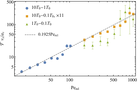
Figure 8: Plot of $\mathcal{T}$, defined in Eq. (60), against Péclet number for our 3 combinations of temperature. The $10T_{0}-0.1T_{0}$ data are multiplied by 11 to account for a their larger factor of $(T_{i}/T_{j})^{1}-1$. Errors shown are 1 standard deviation, and are smaller than the plot markers for many data points.

References

- Wu and Libchaber (2000) X.-L. Wu and A. Libchaber, “Particle diffusion in a quasi-two-dimensional bacterial bath,” Phys. Rev. Lett. 84, 3017–3020 (2000).
- Soni et al. (2003) G. V. Soni, B. M. J. Ali, Y. Hatwalne, and G. V. Shivashankar, “Single particle tracking of correlated bacterial dynamics,” Biophys. J. 84, 2634–2637 (2003).
- Leptos et al. (2009) K. C. Leptos, J. S. Guasto, J. P. Gollub, A. I. Pesci, and R. E. Goldstein, “Dynamics of enhanced tracer diffusion in suspensions of swimming eukaryotic microorganisms,” Phys. Rev. Lett. 103, 198103 (2009).
- Miño et al. (2011) G. Miño, T. E. Mallouk, T. Darnige, M. Hoyos, J. Dauchet, J. Dunstan, R. Soto, Y. Wang, A. Rousselet, and E. Clement, “Enhanced diffusion due to active swimmers at a solid surface,” Phys. Rev. Lett. 106, 048102 (2011).
- Kurtuldu et al. (2011) H. Kurtuldu, J. S. Guasto, K. A. Johnson, and J. P. Gollub, “Enhancement of biomixing by swimming algal cells in two-dimensional films,” Proceedings of the National Academy of Sciences 108, 10391–10395 (2011).
- Valeriani et al. (2011) C. Valeriani, M. Li, J. Novosel, J. Arlt, and D. Marenduzzo, “Colloids in a bacterial bath: simulations and experiments,” Soft Matter 7, 5228–5238 (2011).
- Miño et al. (2013) G. L. Miño, J. Dunstan, A. Rousselet, E. Clément, and R. Soto, “Induced diffusion of tracers in a bacterial suspension: theory and experiments,” Journal of Fluid Mechanics 729, 423–444 (2013).
- Jepson et al. (2013) A. Jepson, V. A. Martinez, J. Schwarz-Linek, A. Morozov, and W. C. K. Poon, “Enhanced diffusion of nonswimmers in a three-dimensional bath of motile bacteria,” Phys. Rev. E 88, 041002 (2013).
- Jeanneret et al. (2016) R. Jeanneret, D. O. Pushkin, V. Kantsler, and M. Polin, “Entrainment dominates the interaction of microalgae with micron-sized objects,” Nature Communications 7, 12518 (2016).
- Mathijssen, Jeanneret, and Polin (2018) A. J. T. M. Mathijssen, R. Jeanneret, and M. Polin, “Universal entrainment mechanism controls contact times with motile cells,” Phys. Rev. Fluids 3, 033103 (2018).
- Underhill, Hernandez-Ortiz, and Graham (2008) P. T. Underhill, J. P. Hernandez-Ortiz, and M. D. Graham, “Diffusion and spatial correlations in suspensions of swimming particles,” Phys. Rev. Lett. 100, 248101 (2008).
- Molina and Yamamoto (2014) J. J. Molina and R. Yamamoto, “Diffusion of colloidal particles in swimming suspensions,” Molecular Physics 112, 1389–1397 (2014).
- Morozov and Marenduzzo (2014) A. Morozov and D. Marenduzzo, “Enhanced diffusion of tracer particles in dilute bacterial suspensions,” Soft Matter 10, 2748–2758 (2014).
- Krafnick and García (2015) R. C. Krafnick and A. E. García, “Impact of hydrodynamics on effective interactions in suspensions of active and passive matter,” Phys. Rev. E 91, 022308 (2015).
- Krishnamurthy and Subramanian (2015) D. Krishnamurthy and G. Subramanian, “Collective motion in a suspension of micro-swimmers that run-and-tumble and rotary diffuse,” Journal of Fluid Mechanics 781, 422–466 (2015).
- de Graaf and Stenhammar (2017) J. de Graaf and J. Stenhammar, “Lattice-Boltzmann simulations of microswimmer-tracer interactions,” Phys. Rev. E 95, 023302 (2017).
- Shum and Yeomans (2017) H. Shum and J. M. Yeomans, “Entrainment and scattering in microswimmer-colloid interactions,” Phys. Rev. Fluids 2, 113101 (2017).
- Harder and Cacciuto (2018) J. Harder and A. Cacciuto, “Hierarchical collective motion of a mixture of active dipolar Janus particles and passive charged colloids in two dimensions,” Phys. Rev. E 97, 022603 (2018).
- Dunkel et al. (2010) J. Dunkel, V. B. Putz, I. M. Zaid, and J. M. Yeomans, “Swimmer-tracer scattering at low Reynolds number,” Soft Matter 6, 4268–4276 (2010).
- Thiffeault and Childress (2010) J.-L. Thiffeault and S. Childress, “Stirring by swimming bodies,” Physics Letters A 374, 3487 – 3490 (2010).
- Eckhardt and Zammert (2012) B. Eckhardt and S. Zammert, “Non-normal tracer diffusion from stirring by swimming microorganisms,” Eur. Phys. J. E 35, 96 (2012).
- Mathijssen, Pushkin, and Yeomans (2015) A. J. T. M. Mathijssen, D. O. Pushkin, and J. M. Yeomans, “Tracer trajectories and displacement due to a micro-swimmer near a surface,” Journal of Fluid Mechanics 773, 498–519 (2015).
- Thiffeault (2015) J.-L. Thiffeault, “Distribution of particle displacements due to swimming microorganisms,” Phys. Rev. E 92, 023023 (2015).
- Suma, Cugliandolo, and Gonnella (2016) A. Suma, L. F. Cugliandolo, and G. Gonnella, “Tracer motion in an active dumbbell fluid,” Journal of Statistical Mechanics: Theory and Experiment 2016, 054029 (2016).
- Burkholder and Brady (2017) E. W. Burkholder and J. F. Brady, “Tracer diffusion in active suspensions,” Phys. Rev. E 95, 052605 (2017).
- Yasuda, Okamoto, and Komura (2017) K. Yasuda, R. Okamoto, and S. Komura, “Anomalous diffusion in viscoelastic media with active force dipoles,” Phys. Rev. E 95, 032417 (2017).
- Mueller and Thiffeault (2017) P. Mueller and J.-L. Thiffeault, “Fluid transport and mixing by an unsteady microswimmer,” Phys. Rev. Fluids 2, 013103 (2017).
- Faxén (1922) H. Faxén, “Der Widerstand gegen die Bewegung einer starren Kugel in einer zähen Flüssigkeit, die zwischen zwei parallelen ebenen Wänden eingeschlossen ist,” Annalen der Physik 373, 89–119 (1922).
- Durlofsky, Brady, and Bossis (1987) L. Durlofsky, J. F. Brady, and G. Bossis, “Dynamic simulation of hydrodynamically interacting particles,” Journal of Fluid Mechanics 180, 21–49 (1987).
- Rotne and Prager (1969) J. Rotne and S. Prager, “Variational treatment of hydrodynamic interaction in polymers,” The Journal of Chemical Physics 50, 4831–4837 (1969).
- Yamakawa (1970) H. Yamakawa, “Transport properties of polymer chains in dilute solution: Hydrodynamic interaction,” The Journal of Chemical Physics 53, 436–443 (1970).
- Kasyap, Koch, and Wu (2014) T. V. Kasyap, D. L. Koch, and M. Wu, “Hydrodynamic tracer diffusion in suspensions of swimming bacteria,” Physics of Fluids 26, 081901 (2014).
- Patteson et al. (2016) A. E. Patteson, A. Gopinath, P. K. Purohit, and P. E. Arratia, “Particle diffusion in active fluids is non-monotonic in size,” Soft Matter 12, 2365–2372 (2016).
- Taylor (1953) G. I. Taylor, “Dispersion of soluble matter in solvent flowing slowly through a tube,” Proceedings of the Royal Society of London. Series A. Mathematical and Physical Sciences 219, 186–203 (1953).
- Pham et al. (2009) T. T. Pham, U. D. Schiller, J. R. Prakash, and B. Dünweg, “Implicit and explicit solvent models for the simulation of a single polymer chain in solution: Lattice Boltzmann versus Brownian dynamics,” The Journal of Chemical Physics 131, 164114 (2009).
- Jain et al. (2012) A. Jain, S. P., B. Dünweg, and J. R. Prakash, “Optimization of a Brownian-dynamics algorithm for semidilute polymer solutions,” Physical Review E 85, 066703 (2012).
- Dyer and Ball (2017) O. T. Dyer and R. C. Ball, “Wavelet Monte Carlo dynamics: A new algorithm for simulating the hydrodynamics of interacting Brownian particles,” The Journal of Chemical Physics 146, 124111 (2017).
- Dyer (2019) O. T. Dyer, Wavelet Monte Carlo dynamics, Ph.D. thesis, University of Warwick (2019).
- Dünweg and Kremer (1993) B. Dünweg and K. Kremer, “Molecular dynamics simulation of a polymer chain in solution,” The Journal of Chemical Physics 99, 6983–6997 (1993).
- Pushkin and Yeomans (2013) D. O. Pushkin and J. M. Yeomans, “Fluid mixing by curved trajectories of microswimmers,” Phys. Rev. Lett. 111, 188101 (2013).
- Green (1954) M. S. Green, “Markoff random processes and the statistical mechanics of time-dependent phenomena. II. Irreversible processes in fluids,” The Journal of Chemical Physics 22, 398–413 (1954).
- Kubo (1957) R. Kubo, “Statistical-mechanical theory of irreversible processes. I. General theory and simple applications to magnetic and conduction problems,” Journal of the Physical Society of Japan 12, 570–586 (1957).
- Happel and Brenner (1973) J. Happel and H. Brenner, Low Reynolds Number Hydrodynamics (Noordhoff,Leyden, 1973).
- Kubo (1966) R. Kubo, “The fluctuation-dissipation theorem,” Reports on Progress in Physics 29, 255–284 (1966).
- Noetinger (1990) B. Noetinger, “Fluctuating hydrodynamics and Brownian motion,” Physica A: Statistical Mechanics and its Applications 163, 545 – 558 (1990).
- Rossky, Doll, and Friedman (1978) P. J. Rossky, J. D. Doll, and H. L. Friedman, “Brownian dynamics as smart Monte Carlo simulation,” The Journal of Chemical Physics 69, 4628–4633 (1978).
- Berg (1993) H. Berg, Random Walks in Biology, Princeton paperbacks (Princeton University Press, 1993).
- Saragosti, Silberzan, and Buguin (2012) J. Saragosti, P. Silberzan, and A. Buguin, “Modeling E. coli tumbles by rotational diffusion. Implications for chemotaxis,” PLOS ONE 7, 1–6 (2012).
- Pushkin, Shum, and Yeomans (2013) D. O. Pushkin, H. Shum, and J. M. Yeomans, “Fluid transport by individual microswimmers,” Journal of Fluid Mechanics 726, 5–25 (2013).
- Crank (1975) J. Crank, The Mathematics of Diffusion, 2nd ed. (Oxford University Press, 1975).