A Computational Study of Perspective Cuts

Abstract

The benefits of cutting planes based on the perspective function are well known for many specific classes of mixed-integer nonlinear programs with on/off structures. However, we are not aware of any empirical studies that evaluate their applicability and computational impact over large, heterogeneous test sets in general-purpose solvers. This paper provides a detailed computational study of perspective cuts within a linear programming based branch-and-cut solver for general mixed-integer nonlinear programs. Within this study, we extend the applicability of perspective cuts from convex to nonconvex nonlinearities. This generalization is achieved by applying a perspective strengthening to valid linear inequalities which separate solutions of linear relaxations. The resulting method can be applied to any constraint where all variables appearing in nonlinear terms are semi-continuous and depend on at least one common indicator variable. Our computational experiments show that adding perspective cuts for convex constraints yields a consistent improvement of performance, and adding perspective cuts for nonconvex constraints reduces branch-and-bound tree sizes and strengthens the root node relaxation, but has no significant impact on the overall mean time.

1 Introduction

Consider a mixed-integer nonlinear program (MINLP) with semi-continuous variables:

$$\min\; \left<\bm{c},(\bm{x},\bm{y},\bm{z})\right>$$ (1a)

s.t. $$g(\bm{x},\bm{y},\bm{z})\leq 0,$$ (1b)

$$(\underline{y}_{j}-y^{0}_{j})z_{k}\leq y_{j}-y^{0}_{j}\leq(\overline{y}_{j}-y^{0}_{j})z_{k},~{}\forall j\in\mathcal{S}_{k},~{}\forall k\in\mathcal{I},$$ (1c)

$$\bm{x}\in\mathbb{R}^{n},~{}\bm{y}\in\mathbb{R}^{p},~{}\bm{z}\in\{0,1\}^{q}.$$ (1d)

Here, $\left<\bm{c},(\bm{x},\bm{y},\bm{z})\right>$ is the linear objective function given by a scalar product of a constant vector $\bm{c}\in\mathbb{R}^{n+p+q}$ and the vectors of continuous variables $\bm{x}$, semi-continuous variables $\bm{y}$ and binary variables $\bm{z}$. Constraints (1b) are given by inequalities $g(\bm{x},\bm{y},\bm{z})\leq 0$, where $g:~{}\mathbb{R}^{n}\times\mathbb{R}^{p}\times[0,1]^{q}\rightarrow\mathbb{R}^{m}$ is a vector function and some of its elements $g_{i}$ are nonlinear.

The set $\mathcal{S}_{k}\subseteq\{1,\ldots,p\}$ shall contain the indices of semi-continuous variables controlled by the indicator variable $z_{k}$, and $\mathcal{I}\subseteq\{1,\dots,q\}$ is the set of indices of all indicator variables. Constraints (1c) ensure that for each $j\in\mathcal{S}_{k}$, the value of $y_{j}$ belongs to the domain $[\underline{y}_{j},\overline{y}_{j}]$ when the indicator variable $z_{k}$ is equal to $1$ and has a fixed value $y^{0}_{j}$ when $z_{k}$ is equal to $0$. Semi-continuous variables are typically used to model “on” and “off” states of a process and can be found in such problems as optimal line switching in electrical networks [7], blending [24] and production planning [3], to name but a few.

In order to simplify the notation, in the rest of the paper the subscript $k$ will be omitted and we will be referring to a vector of semi-continuous variables $\bm{y}\in\mathbb{R}^{p}$ controlled by the indicator variable $z\in\{0,1\}$. The semi-continuity relation is then defined by the inequality $(\underline{\bm{y}}-\bm{y}^{0})z\leq\bm{y}-\bm{y}^{0}\leq(\overline{\bm{y}}-\bm{y}^{0})z.$

Without loss of generality, we consider constraints of the form

$$g(\bm{x},\bm{y})=f(\bm{y})-x_{\ell}\leq 0$$ (2)

for some $\ell\in\{1,\ldots,n\}$. The continuous variable $x_{\ell}$ represents the linear non-semi-continuous part and the same arguments as presented in this paper can be directly adapted for a more general linear part. When $z=0$, function $f$ is reduced to a fixed value $f(\bm{y}^{0})$. A common example of such constraints are on/off constraints which become redundant when the corresponding indicator variable is set to $0$.

Many state-of-the-art algorithms for the solution of MINLP (1) make use of nonlinear and linear programming relaxations where the condition $z\in\{0,1\}$ is replaced with $z\in[0,1]$. However, for a constraint of the form (2), simply dropping the integrality condition generally does not produce the tightest possible continuous relaxation. The reason for this is that the dependence of the bounds on $\bm{y}$ on the indicator variable $z$ is not exploited by a straightforward continuous relaxation. Consequently, the same applies for the linearization of Constraint (2) via gradient cuts [16], that is, inequalities

$$f(\hat{\bm{y}})+\left<\nabla f(\hat{\bm{y}}),\bm{y}-\hat{\bm{y}}\right>\leq x_{\ell},$$ (3)

where $\hat{\bm{y}}$ is the point at which $f$ is linearized.

The strongest continuous relaxation of the set described by Constraint (2), given that $\bm{y}$ is semi-continuous, can be achieved by applying the perspective reformulation [9]. Linearizing this reformulation provides valid linear inequalities known as perspective cuts.

In this paper we present a computational study of perspective cuts within SCIP [12], a general-purpose solver that implements an LP-based branch-and-cut algorithm to solve mixed-integer nonlinear programs to global optimality. Section 2 provides the theoretical background for this study and a review of applications that can be found in existing literature. In Section 3, we describe our approach to creating perspective cuts and show that for convex instances, it is equivalent to linearizing the perspective formulation via gradient cuts. Section 4 gives an outline of our implementation of perspective cuts in SCIP, which includes detection of suitable structures and separation and strengthening of perspective cuts. Finally, in Section 5 the results of computational experiments on instances from MINLPLib [4] are presented.

2 Perspective Formulations for Convex Nonlinearities

This section gives a review of the existing literature on theoretical and computational results related to perspective formulations for convex nonlinearities.

2.1 Theoretical background

Let $F$ denote the feasible region defined by Constraint (2) and the semi-continuity constraints (1c) for an indicator $z$. $F$ can be written as a union of two sets $F^{0}$ and $F^{1}$ corresponding to values $0$ and $1$ of $z$, respectively:

$$F^{0}=\{(x_{\ell},\bm{y},z)~{}|~{}x_{\ell}\geq f(\bm{y}^{0}),~{}\bm{y}=\bm{y}^{0},~{}z=0\},$$ (4)

$$F^{1}=\{(x_{\ell},\bm{y},z)~{}|~{}x_{\ell}\geq f(\bm{y}),~{}\bm{y}\in[\underline{\bm{y}},\overline{\bm{y}}],~{}z=1\}.$$ (5)

The tightest possible convex relaxation of $F$ is its convex hull. Ceria and Soares [5] studied convex hull formulations for unions of convex sets and their applications to disjunctive programming. Stubbs and Mehrotra [21] described the convex hull of the feasible set of a convex 0-1 program and developed a procedure for generating cutting planes. Grossmann and Lee [13] extended the convex hull results to generalized disjunctive programs (GDPs). Similarly to disjunctive programming, feasible sets of GDPs are given as unions of convex sets, but more general logical relations are also allowed. These works used the perspective function, which is defined as follows:

Definition 1.

[18] For a given convex function $f:\mathbb{R}^{p}\rightarrow\mathbb{R}$, its perspective function $\tilde{f}:\mathbb{R}^{n+1}\rightarrow\left(\mathbb{R}\cup\{+\infty\}\right)$ is defined as:

$$\tilde{f}(\bm{y},z)=\begin{cases}zf(\bm{y}/z),&\text{ if }z>0,\\ +\infty,&\text{ otherwise,}\end{cases}$$

where $\bm{y}\in\mathbb{R}^{p}$, $z\in\mathbb{R}$.

These early results are applicable to convex sets with few non-restrictive conditions and utilize an extended variable space. Frangioni and Gentile [9] proposed a reformulation in the original space for a special case. Considering a semi-continuous vector $\bm{y}$, an indicator variable $z$, and a convex function $f$ depending only on $\bm{y}$ such that $\bm{y}^{0}=(0,\dots,0)$ and $f(\bm{0})=0$, they capture the disjunctive structure by defining a new nonconvex function $f^{d}$:

$$f^{d}(\bm{y},z)=\begin{cases}f(\bm{y})&\text{ if }z=1,~{}y\in[\underline{\bm{y}},\overline{\bm{y}}],\\ 0&\text{ if }\bm{y}=z=0,\\ +\infty&\text{ otherwise.}\end{cases}$$

The function $f^{d}$ is directly related to the set $F$: the latter can be described as the set of all points $(x_{\ell},\bm{y},z)$ such that $f^{d}(\bm{y},z)$ is finite and $f^{d}(\bm{y},z)\leq x_{\ell}$. Frangioni and Gentile describe the convex envelope of $f^{d}$:

$$\overline{co}f^{d}(\bm{y},z)=\begin{cases}\tilde{f}(\bm{y},z)&\text{ if }z\in(0,1],\\ 0&\text{ if }z=0,\\ +\infty&\text{ otherwise.}\end{cases}$$

In a related work, Günlük and Linderoth [14] show that the convex hull of $F$ is given by

$$\text{conv}(F)=\{(x_{\ell},\bm{y},z)~{}|~{}\overline{co}f^{d}(\bm{y},z) \leq x_{\ell},$$

$$(\underline{\bm{y}}-\bm{y}^{0})z \leq\bm{y}-\bm{y}^{0}\leq(\overline{\bm{y}}-\bm{y}^{0})z,~{}z\in[0,1]\}.$$ (6)

Therefore, replacing $f$ with $\overline{co}f^{d}$ in Constraint (2) results in a reformulation with the tightest possible continuous relaxation: the perspective reformulation. This is a valid reformulation since $f=\overline{co}f^{d}$ for $z\in\{0,1\}$.

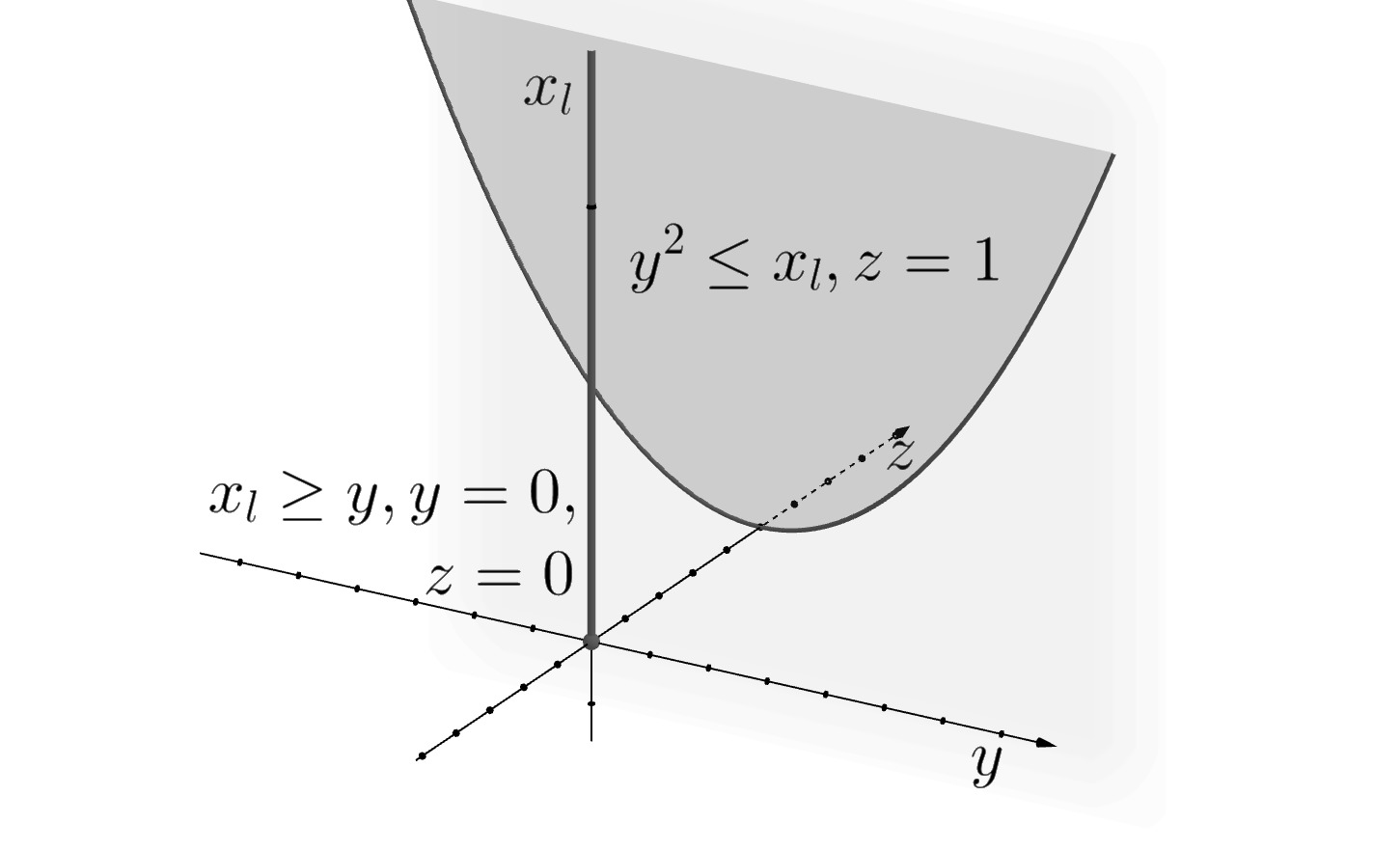
(a) the mixed-integer set

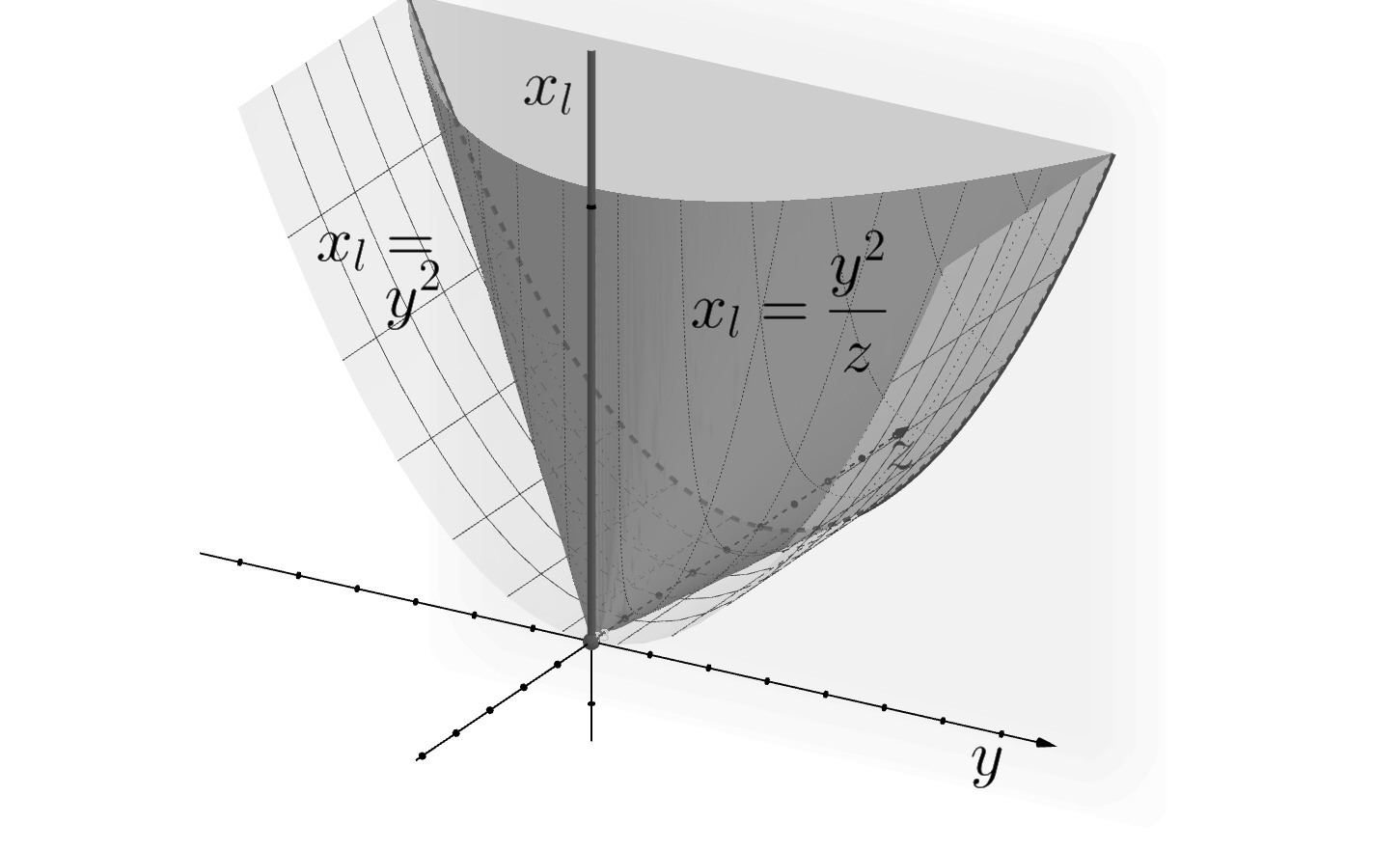
(b) the continuous relaxations

Figure 1: Example of a disjunctive set and its convex hull

Figure 1 shows an example of a disjunctive set and compares its continuous relaxations. The disjunctive set (shown in Figure 1(a)) consists of the ray $\{(x_{\ell},y,z)~{}|~{}x_{\ell}\geq 0,~{}y=0,~{}z=0\}$ and the convex set $\{(x_{\ell},y,z)~{}|~{}x_{\ell}\geq f(y),~{}z=1\}$, where $f(y)=y^{2}$. The convex hull, shown in Figure 1(b), is the closure of the set of all points above the dark gray surface defined by $x_{\ell}=y^{2}/z$, $z\in(0,1]$. This equation is obtained by applying the perspective operator to $f$: $\tilde{f}(y,z)=zf(y/z)=y^{2}/z$. For comparison, the boundary of the straightforward continuous relaxation given by $x_{\ell}=y^{2}$, $z\in[0,1]$, is shown in Figure 1(b) in light gray color.

Due to the division by $z$ in the perspective function, the perspective reformulation (6) is non-differentiable at $z=0$. In some special cases, formulation (6) can be written as a second-order cone (SOC) constraint [22, 1, 14, 10]. In particular, this is possible when Constraint (2) itself is SOC-representable.

Frangioni and Gentile [11, 8] introduced projection approaches for additively separable closed convex functions. In the projected perspective reformulation (P²R) [11], the perspective function is projected into the space of continuous variables and rewritten as a piecewise-convex function. This technique avoids the numerical issues associated with the perspective functions while yielding strong bounds, but at the cost of using piecewise-continuous functions which cannot be directly passed to off-the-shelf solvers. The approximated projected perspective reformulation (AP²R) method [8] lifts the P²R formulation back into the original space by reintroducing the indicator variables. AP²R can be solved by general-purpose solvers and, if $\bm{y}^{0}\leq\underline{\bm{y}}$, has the same number of variables and constraints as the original problem. The bound provided by AP²R is, however, generally weaker than the one from P²R.

Alternatively, the perspective reformulation (6) can be represented by an infinite number of linear outer approximations which are then dynamically separated. Suppose that we have a point $(\hat{x}_{\ell},\hat{\bm{y}},\hat{z})$ such that $\hat{z}\in(0,1)$ and $\hat{x}_{\ell}<\tilde{f}(\hat{\bm{y}},\hat{z})$. By performing first-order analysis of the convex envelope $\overline{co}f^{d}$, Frangioni and Gentile [9] derive cuts that separate $(\hat{x}_{\ell},\hat{\bm{y}},\hat{z})$ from the convex hull of $F$, referred to as perspective cuts:

$$\left<\nabla f(\bm{y}^{*}),\bm{y}\right>+\left(f(\bm{y}^{*})-\left<\nabla f(\bm{y}^{*}),\bm{y}^{*}\right>\right)z\leq x_{\ell},$$ (7)

where $\bm{y}^{*}=\hat{\bm{y}}/\hat{z}$.

It is easy to adjust the perspective reformulation and the inequalities (7) for the case of nonzero $\bm{y}^{0}$ and $f(\bm{y}^{0})$:

$$\left<\nabla f(\bm{y}^{*}),\bm{y}-\bm{y}^{0}\right>+(f(\bm{y}^{*})-f(\bm{y}^{0})-\left<\nabla f(\bm{y}^{*}),\bm{y}^{*}-\bm{y}^{0}\right>)z+f(\bm{y}^{0})\leq x_{\ell},$$ (8)

where $\bm{y}^{*}=(\hat{\bm{y}}-\bm{y}^{0})/\hat{z}+\bm{y}^{0}$. We refer to (8) as the perspective cut at $\bm{y}^{*}$.

2.2 Existing applications and computational results

Perspective cuts and reformulations were tested on several applications which contain convex functions of semi-continuous variables.

Frangioni and Gentile [9] applied perspective cuts (8) to the thermal unit commitment problem. In order to avoid the technical difficulties of incorporating perspective cuts into a general-purpose solver, the authors implemented their own NLP-based branch-and-cut algorithm. Perspective cuts are applied to the objective function via a specialized separation procedure, which replaces a univariate term with its perspective linearization if the perspective linearization is tighter at the current relaxation solution. The linearization is represented by an auxiliary variable, and as more perspective cuts are added for the term, the variable is set to be equal to the maximum of all linearizations. Perspective cuts were shown to have a considerable impact on the performance. The geometric mean of the running time of the best performing setting was smaller than that for the algorithm with the straightforward continuous relaxation by a factor of $60$.

Perspective reformulations were studied by Günlük and Linderoth [14, 15]. Their key observation is that for some problems, the perspective reformulation can be written with the use of second-order cone constraints. The applications studied in this paper are:

• Separable quadratic uncapacitated facility location on a testset consisting of $16$ instances. With the perspective reformulation, $50\%$ more instances are solved within the time limit of $8$ hours and on the instances that are solved with both formulations, the perspective formulation is faster by a factor of $8$ when comparing the geometric mean.

• Network design with congestion constraints on a testset consisting of $35$ instances. The perspective formulation is solved for 29 instances within the time limit of $4$ hours, as opposed to only 2 instances with the standard formulation.

• Mean-variance optimization (portfolio optimization) on a testset consisting of $20$ instances. Although none of the instances are solved within the time limit of 10,000 CPU seconds, perspective reformulation significantly improves the gap. For example, the final gap between the best found lower and upper bounds is reduced from $185.1\%$ with the standard formulation to $4.2\%$ with the perspective reformulation on instances of smaller size, and from $490.0\%$ to $5.9\%$ on instances of larger size.

Atamtürk and Gómez [2] applied the perspective-based conic reformulation to the image segmentation problem, testing it on $4$ instances of different sizes. On the one instance that was solved within a time limit of $1$ hour, the running time was reduced by a factor of $18$ when compared to the standard formulation. On the three remaining instances, using the perspective formulation resulted in a $45$-$55\%$ decrease of the remaining gap at time limit.

Aktürk et al. [1] presented a perspective-based conic reformulation of the machine-job assignment problem with controllable processing times. The tests were conducted on 180 randomly generated instances of varying sizes with quadratic and cubic objectives. For problems with a quadratic objective, 91% of the 90 instances were solved when using the strengthened conic formulation, whereas at most 36% of instances were solved when using non-perspective formulations. For problems with a cubic objective, 88% of the 90 instances were solved with the perspective formulation and at most 27% were solved with non-perspective formulations.

A comparison between SOC-based perspective formulations and perspective cutting planes was performed by Frangioni and Gentile [10]. Using the CPLEX-11 solver, they test the two approaches on two sets of mixed-integer quadratic problems, namely, the Markowitz mean-variance model and the unit commitment problem. The difference between the two formulations is particularly significant with the setup used in the paper [10] since by default, CPLEX obtains dual bounds by solving nonlinear relaxations. The results favor the cutting planes approach, with the difference being larger for the Markowitz mean-variance problem. The authors observe that the advantage of perspective cuts stems mostly from efficient reoptimization of linear programs. They add that the perspective conic reformulation is more competitive for problems that are larger, more nonlinear (i.e., have more nonlinear constraints or non-quadratic nonlinear constraints) or have richer structure.

Frangioni and Gentile [11, 8] tested the projected perspective reformulation (P²R) and the approximated perspective projected reformulation (AP²R) on sensor placement, nonlinear network design, mean-variance portfolio and unit commitment problems. P²R was implemented as part of a specialized branch-and-bound algorithm and AP²R was solved directly with CPLEX 12. Both approaches were compared to perspective cuts implemented as a callback in CPLEX. Computational results show that P²R is the best performing method for problems that have a well-suited structure and require little or no branching. For problems with more complex structures, AP²R is competitive with the perspective cut approach. When there are constraints linking indicator variables and few linear approximations provide a good estimate of the original nonlinear function, perspective cuts tend to be the best performing method.

Salgado et al. [19] studied the alternating current optimal power flow problem with activation/deactivation of generators (ACOPFG) using $8$ test instances. They tested two perspective-based reformulations of the objective function. The first uses four perspective cuts of the form (8); the other is obtained by applying AP²R [8]. Although the results of enhancing the standard ACOPFG model with perspective reformulations are inconclusive, an outer approximation [20] of the problem significantly benefits from both perspective cuts and AP²R. The perspective cuts approach performs best, solving one more instance than the standard formulation within the time limit of $1$ hour and taking less than $4$ seconds on all the remaining instances, whereas the standard formulation requires over $1000$ seconds on most instances.

3 Generalized perspective cuts

If $f$ is non-convex, neither the gradient cuts (3) nor the perspective cuts (8) are guaranteed to be valid. However, the perspective reformulation can be applied to a convex underestimator of $f$, from which the perspective cuts (8) can be derived. Alternatively, any linear inequality $\phi(\bm{y})\leq x_{\ell}$ that is valid for the ‘on’ set $F^{1}$ can be adjusted for the ‘off’ set $F^{0}$.

In the following, we propose a cut extension procedure that ensures that the generated inequality is equivalent to $\phi(\bm{y})\leq x_{\ell}$ when the indicator is equal to $1$ and holds with equality at the point $(x_{\ell},\bm{y},z)=(f(\bm{y}^{0}),\bm{y}^{0},0)$.

Theorem 1 (Generalized perspective cuts).

Consider a vector of semi-continuous variables $\bm{y}\in\mathbb{R}^{p}$ with an indicator $z\in\{0,1\}$, such that $\bm{y}=\bm{y}^{0}$ if $z=0$, and a linear inequality $\phi(\bm{y})\leq x_{\ell}$ that is valid for the set

$$F^{1}=\{(x_{\ell},\bm{y},z)~{}|~{}x_{\ell}\geq f(\bm{y}),~{}\bm{y}\in[\underline{\bm{y}},\overline{\bm{y}}],~{}z=1\}.$$

Let

$$\tilde{\phi}(\bm{y},z)=\phi(\bm{y})+\left(f(\bm{y}^{0})-\phi(\bm{y}^{0})\right)(1-z).$$

Then the linear inequality $\tilde{\phi}(\bm{y},z)\leq x_{\ell}$ is valid for the set $F^{0}\cup F^{1}$, where

$$F^{0}=\{(x_{\ell},\bm{y},z)~{}|~{}~{}x_{\ell}\geq f(\bm{y}^{0}),~{}\bm{y}=\bm{y}^{0},~{}z=0\}.$$

Proof.

It is sufficient to check the validity for each possible value of $z\in\{0,1\}$. By substituting $z=1$ and $z=0$ in $\tilde{\phi}(\bm{y},z)$, we immediately obtain

1. $\tilde{\phi}(\bm{y},1)=\phi(\bm{y})~{}\forall\bm{y}\in\mathbb{R}^{p}$ and

2. $\tilde{\phi}(\bm{y}^{0},0)=f(\bm{y}^{0})$,

respectively. Therefore, $\tilde{\phi}(\bm{y},z)\leq x_{\ell}$ is a valid inequality. ∎∎

If the cut $\phi(\bm{y})\leq x_{\ell}$ is already valid for $F^{0}$, then the described above adjustment always produces a cut that is at least as strong as the original cut. Since $\phi(\bm{y})\leq x_{\ell}$ is in this case implied by $f(\bm{y})\leq x_{\ell}$ for $(x_{\ell},\bm{y})\in F^{0}$, we have $\phi(\bm{y}^{0})\leq f(\bm{y}^{0})$. Hence the coefficient of $(1-z)$ in $\tilde{\phi}(\bm{y},z)$ is nonnegative and

$$\tilde{\phi}(\bm{y},z)\geq\phi(\bm{y}),~{}\forall z\in[0,1],~{}\forall\bm{y}\in\mathbb{R}^{p}.$$

If additionally $\phi(\bm{y}^{0})<f(\bm{y}^{0})$, i.e., the original cut is not tight at $\bm{y}^{0}$, then the new cut is also stronger. Otherwise, if $\phi(\bm{y})\leq x_{\ell}$ does not hold for $F^{0}$ (that is, if $\phi(\bm{y}^{0})>f(\bm{y}^{0})$), then the adjustment is necessary to obtain a cut that is valid for $F^{0}\cup F^{1}$.

This cut extension procedure has two main advantages:

1. It does not depend on the convexity of $f$ and requires no assumptions on the cut except for its validity for $F^{1}$.

2. In the case where $\bm{y}^{0}\notin[\underline{\bm{y}},\overline{\bm{y}}]$, variable bounds for $F^{1}$ are tighter than those for $F^{0}\cup F^{1}$. This is useful for non-convex constraints since the tightness of their relaxations depends on variable bounds, and therefore cuts constructed for $\bm{y}\in[\underline{\bm{y}},\overline{\bm{y}}]$ will generally be stronger than those for $\bm{y}\in[\min\{\bm{y}^{0},\underline{\bm{y}}\},\max\{\bm{y}^{0},\overline{\bm{y}}\}]$.

When the cut strengthening is applied to the convex setting, the result is equivalent to the well-known perspective cuts:

Theorem 2 (Alternative derivation of perspective cuts).

Suppose that $f:\mathbb{R}^{p}\rightarrow\mathbb{R}$ is convex and $(\hat{x}_{\ell},\hat{\bm{y}},\hat{z})\not\in\text{conv}(F)$ as defined in Section 2.1. Consider the gradient cut (3) at point $\bm{y}^{*}=(\hat{\bm{y}}-\bm{y}^{0})/\hat{z}+\bm{y}^{0}$ for Constraint (2):

$$\phi(\bm{y})=f(\bm{y}^{*})+\left<\nabla f(\bm{y}^{*}),\bm{y}-\bm{y}^{*}\right>\leq x_{\ell}.$$

Let $\tilde{\phi}(\bm{y},z)$ be the linear function obtained from $\phi(\bm{y})$ by following the strengthening procedure in Theorem 1. Then $\tilde{\phi}(\bm{y},z)$ is written as follows:

$$\tilde{\phi}(\bm{y},z)=\left<\nabla f(\bm{y}^{*}),\bm{y}-\bm{y}^{0}\right>+(f(\bm{y}^{*})-f(\bm{y}^{0})-\left<\nabla f(\bm{y}^{*}),\bm{y}^{*}-\bm{y}^{0}\right>)z+f(\bm{y}^{0})$$

and the cut $\tilde{\phi}(\bm{y},z)\leq x_{\ell}$ is equivalent to the perspective cut (8) at point $(\hat{\bm{y}},\hat{z})$.

Proof.

The coefficient of $(1-z)$ in $\tilde{\phi}(\bm{y},z)$ is

$$\alpha=f(\bm{y}^{0})-\phi(\bm{y}^{0})=f(\bm{y}^{0})-f(\bm{y}^{*})-\left<\nabla f(\bm{y}^{*}),\bm{y}^{0}-\bm{y}^{*}\right>.$$

Adding $\alpha(1-z)$ to the left hand side of the gradient cut produces the perspective cut (8):

$$\tilde{\phi}(\bm{y},z)=\phi(\bm{y})+\alpha(1-z)=$$

$$\left<\nabla f(\bm{y}^{*}),\bm{y}-\bm{y}^{0}\right>+(f(\bm{y}^{*})-f(\bm{y}^{0})-\left<\nabla f(\bm{y}^{*}),\bm{y}^{*}-\bm{y}^{0}\right>)z+f(\bm{y}^{0}).$$

∎∎

To paraphrase, for a convex function $f$ the perspective cut at a solution $(\hat{x}_{\ell},\hat{\bm{y}},\hat{z})$ of the LP relaxation can equivalently be obtained by first generating a gradient cut for $f$ at the modified point $\bm{y}^{*}$ and then applying the strengthening procedure from Theorem 1.

Let us consider an example to illustrate the cut extension method.

Example 1.

Consider a constraint $f(y)=-y^{3}+y\leq x_{\ell}$. The boundary of the feasible region is shown in Figure 2 by the dark gray nonlinear surface, and the feasible points are located above it. Let $0.5z\leq y\leq z$, where $y$ is a scalar, semi-continuous variable modeled using the binary variable $z\in\{0,1\}$.

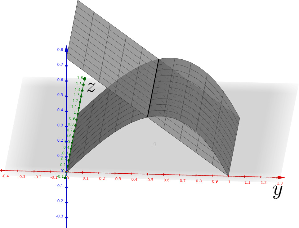
(a) original cut valid for $z=1$, $y\in[0.5,1]$

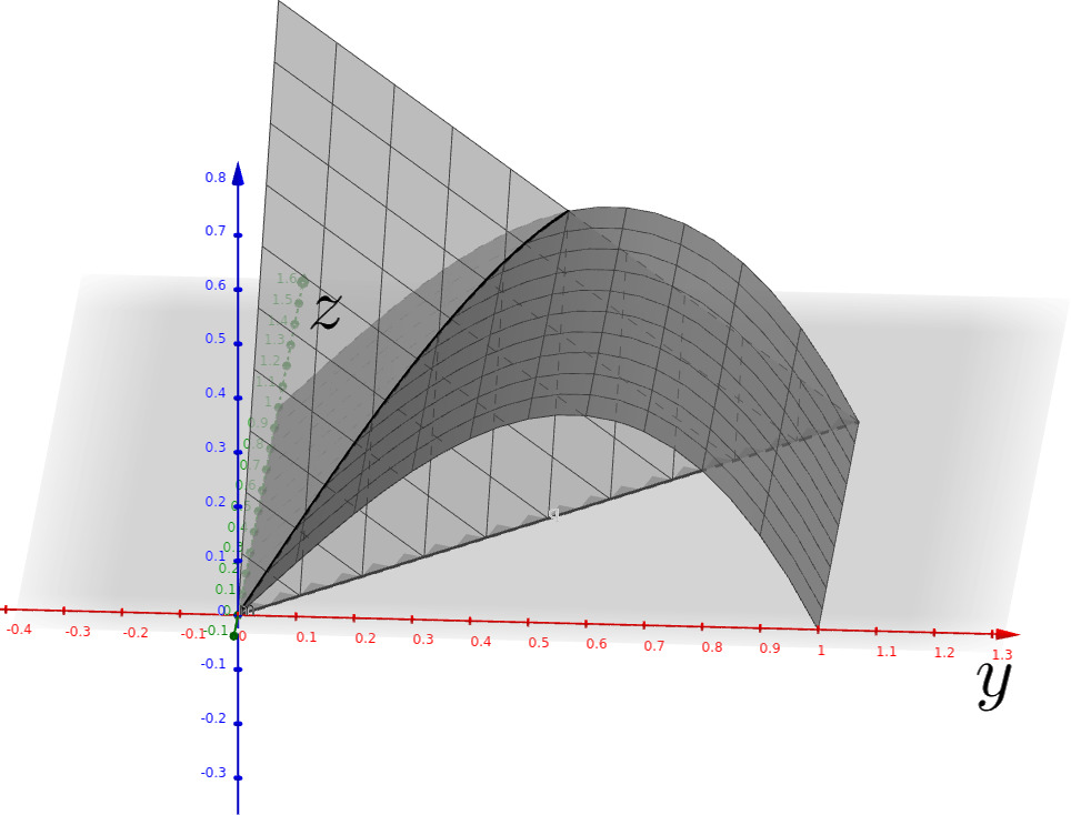
(b) generalized perspective cut

Figure 2: Example of cut extension

First we find an underestimator of $f(y)$ valid for $z=1$. In this case, $y$ is constrained to belong to the interval $[0.5,1]$. Since $f(y)$ is concave on $[0.5,1]$, the underestimator is the secant through points $(0.5,f(0.5))$ and $(1,f(1))$:

$$f^{sec}(y)=-0.75y+0.75.$$

The cut $f^{sec}\leq x_{\ell}$ (shown in Figure 2(a)) is not valid for the whole feasible set. In particular, a feasible point $(y,z,x_{\ell})=(0,0,0)$ violates the cut: $f^{sec}(0,0)=0.75>0=x_{\ell}$.

Now we extend the cut so that to ensure validity at $z=0$. By Theorem 1, the new cut is written as:

$$\tilde{f}^{sec}=f^{sec}+(f(y^{0})-f^{sec}(y^{0}))(1-z)=-0.75y+0.75z.$$

This cut, shown in Figure 2(b), is valid for the whole feasible set given by the cubic constraint and the semi-continuity condition.

4 Implementation of perspective cuts

An effective implementation of perspective cuts within a general-purpose solver requires providing methods for detecting suitable structures in a general problem and generating the cuts during the solution process. In the following, we describe our implementation within SCIP, but many considerations discussed here will be applicable to MINLP solvers in general.

4.1 Organization of nonlinear constraints in SCIP

SCIP builds a relaxation for the MINLP (1) by means of an extended formulation, where auxiliary variables $\bm{w}$ are introduced for the subexpressions that constitute the constraint functions $g(\bm{x},\bm{y},\bm{z})$. Without loss of generality, we can assume that (1b) has been replaced by a new system

$$h_{i}(\bm{x},\bm{y},w_{1},\ldots,w_{i-1},\bm{z})\lesseqqgtr w_{i},\qquad i=1,\ldots,m^{\prime},$$ (9)

$$\bm{w}^{\ell}\leq\bm{w}\leq\bm{w}^{u},$$

where $\bm{w}^{l}$ and $\bm{w}^{u}$ denote global lower and upper bounds on $\bm{w}$.

The handling of nonlinear constraints in the version of SCIP used for this work is performed by modules called “nonlinearity handlers”. Each nonlinearity handler works on a specific structure (e.g. quadratic, convex, etc.) and provides callback methods. For the purposes of this paper, three types of callbacks are relevant:

• Detection callbacks receive an expression and determine whether it is suitable for the nonlinearity handler.

• Estimation callbacks provide linear under- and overestimators given an expression and a point at which to linearize it.

• Enforcement callbacks enforce a given violated constraint by adding cutting planes, tightening bounds, detecting infeasibility, etc.

Our addition of generalized perspective cuts is implemented via a specialized perspective nonlinearity handler.

4.2 Structure detection

The detection algorithm identifies constraints of the form (9), where $h_{i}$ is nonlinear and at least one other nonlinearity handler provides an estimation callback for it. All variables that $h_{i}$ depends on must be semi-continuous with at least one common indicator variable. If several binary variables satisfying this condition are found, all such variables are stored for use in cut generation.

A special case is that of $h_{i}$ being a sum. Here, only the variables appearing in nonlinear terms of the sum are required to be semi-continuous.

To determine whether a variable $y_{j}$ is semi-continuous, the detection callback of the perspective nonlinearity handler searches for pairs of implied bounds on $y_{j}$ with the same indicator $z_{k}$:

$$y_{j} \leq\alpha^{(u)}z_{k}+\beta^{(u)},$$

$$y_{j} \geq\alpha^{(\ell)}z_{k}+\beta^{(\ell)}.$$

If $\beta^{(u)}=\beta^{(\ell)}$, then $y_{j}$ is a semi-continuous variable and $y_{j}^{0}=\beta^{(u)}$, $\underline{y}_{j}=\alpha^{(\ell)}+\beta^{(\ell)}$ and $\overline{y}_{j}=\alpha^{(u)}+\beta^{(u)}$.

This information can be obtained either directly from linear constraints in $y_{j}$ and $z_{k}$, or by finding implicit relations between $y_{j}$ and $z_{k}$. Such relations can be detected by probing, which fixes $z_{k}$ to its possible values and propagates all constraints in the problem, thus detecting implications of $z_{k}=0$ and $z_{k}=1$. SCIP stores the implied bounds in a globally available data structure.

In addition, the perspective nonlinearity handler detects semi-continuous auxiliary variables, that is, variables $w_{i}$ that were introduced to express the extended formulation (9). Given $h_{i}(\bm{y},w_{1},\ldots,w_{i-1})\lesseqqgtr w_{i}$, where $\bm{y},w_{1},\ldots,w_{i-1}$ are semi-continuous variables depending on the same indicator $z_{k}$, the auxiliary variable $w_{i}$ is semi-continuous with $w_{i}^{0}=h_{i}(\bm{y}^{0},w^{0}_{1},\ldots,w^{0}_{i-1})$ and $[\underline{w}_{i},\overline{w}_{i}]=h_{i}([\underline{\bm{y}}^{0},\overline{\bm{y}}^{0}],[\underline{w}_{1},\overline{w}_{1}],\ldots,[\underline{w}_{i-1},\overline{w}_{i-1}])$ computed by interval arithmetics.

According to Theorem 1, the constraint must have the form

$$w_{i}\geq h_{i}(\bm{y},w_{1},\ldots,w_{i-1}),$$

where all variables $\bm{y},w_{1},\ldots,w_{i-1}$ are semi-continuous with respect to the same indicator $z_{k}$. In our implementation we allow a more general form:

$$h_{i}(\bm{x},\bm{y},w_{1},\ldots,w_{i-1},\bm{z}) =h^{sc}_{i,k}(\bm{y},w_{1},\ldots,w_{r})$$ (10)

$$+h^{nsc}_{i,k}(\bm{x},w_{r+1},\ldots,w_{i-1},\bm{z})\lesseqqgtr w_{i},$$

where the variables are assumed to be sorted so that semi-continuous auxiliary variables $w_{1},\ldots,w_{r}$ come before the non-semi-continuous auxiliary variables $w_{r+1},\ldots,w_{i-1}$ and the auxiliary variable $w_{i}$ representing $h_{i}$.

Thus, for each suitable indicator $z_{k}$ the function $h_{i}$ is split up into the semi-continuous part $h^{sc}_{i,k}$, which can depend only on variables that are semi-continuous with respect to indicator $z_{k}$, and a non-semi-continuous part $h^{nsc}_{i,k}$, which depends on non-semi-continuous variables. The non-semi-continuous part must be linear. If the sum has a constant term, the constant is considered to be part of $h^{sc}_{i,k}$.

4.3 Separation and strengthening of generalized perspective cuts

During the cut generation loop, generalized perspective cuts as in Theorem 1 are constructed for constraints of the form (10).

In the following, let $\bm{v}$ denote the vector of all problem variables: $\bm{v}=(\bm{x},\bm{y},\bm{w},\bm{z})$, and let $F^{1}_{i,k}$ and $F^{0}_{i,k}$ be the sets of points satisfying a constraint of the form (10) for a given $i\in\{1,\ldots,m^{\prime}\}$ together with implied variable bounds for $z_{k}=1$ and $z_{k}=0$, respectively. For simplicity, we fix the inequality sign and consider “less than or equal to” constraints:

$$F^{1}_{i}= \{\bm{v}\,|\,h_{i}(\bm{x},\bm{y},w_{1},\ldots,w_{i-1},\bm{z})\leq w_{i},\bm{y}\in[\underline{\bm{y}},\overline{\bm{y}}],\bm{w}\in[\underline{\bm{w}},\overline{\bm{w}}],z_{k}=1\},$$

$$F^{0}_{i}= \{\bm{v}\,|\,h_{i}(\bm{x},\bm{y},w_{1},\ldots,w_{i-1},\bm{z})\leq w_{i},\bm{y}=\bm{y}^{0},\bm{w}=\bm{w}^{0},z_{k}=0\}.$$

Suppose that the point $\hat{\bm{v}}$ violates the nonlinear constraint:

$$h_{i}(\hat{\bm{x}},\hat{\bm{y}},\hat{w}_{1},\ldots,\hat{w}_{i-1},\hat{\bm{z}})>\hat{w}_{i}.$$

If $h_{i}$ is nonconvex and its estimators depend on variable bounds, the enforcement callback first performs probing for $z_{k}=1$ in order to tighten the implied bounds $[\underline{\bm{y}},\overline{\bm{y}}]$ and $[\underline{w}_{j},\overline{w}_{j}]$ for $j\leq r$.

Estimation callbacks of non-perspective nonlinearity handlers are called in order to find valid cuts that separate $\hat{\bm{v}}$ from $F^{1}_{i,k}$, which are then modified according to Theorem 1. For a constraint of the generalized form $h_{i}=h^{sc}_{i,k}+h^{nsc}_{i,k}\leq w_{i}$, which is described in Section 4.2, an estimation callback will provide an underestimator of $h_{i}$:

$$\underline{h}_{i}=\underline{h}^{sc}_{i,k}+h^{nsc}_{i,k}.$$

This underestimator consists of an underestimator of the semi-continuous part $\underline{h}^{sc}_{i,k}$ and the non-semi-continuous part $h^{nsc}_{i,k}$, which remains unchanged since it is already linear and shares none of the variables with the semi-continuous part. The extension procedure from Theorem 1 is applied only to $\underline{h}^{sc}_{i,k}$ to obtain $\underline{\tilde{h}}^{sc}_{i,k}$. Since $h^{sc}_{i,k}$ depends only on semi-continuous variables, similar arguments to Section 3 hold for feasibility and tightness of the strengthened underestimator $\underline{\tilde{h}}^{sc}_{i,k}$. The strengthened underestimator of $h_{i}$ is then written as

$$\underline{\tilde{h}}_{i,k}=\underline{\tilde{h}}^{sc}_{i,k}+h^{nsc}_{i,k}.$$

If $\hat{\bm{v}}$ violates the cut $\underline{\tilde{h}}_{i,k}\leq w_{i}$, the cut is passed to the SCIP core where it will be considered for addition to the LP relaxation.

Let us consider an example of generalized perspective cut separation by extending Example 1.

Example 2.

The extended formulation of the constraint from Example 1 is written as:

$$h(x_{l},y)=-y^{3}+y-x_{l}\leq w\leq 0.$$

The semi-continuous part of $h$ is $h^{sc}(y)=-y^{3}+y$, and the non-semi-continuous part is $h^{nsc}(x_{l})=-x_{l}$. The perspective underestimator of $h$ is $\underline{h}(x_{l},y,z)=-0.75y+0.75z-x_{l}$ and the perspective cut is written as follows:

$$-0.75y+0.75z-x_{l}\leq w.$$

Suppose that the point to be separated is $(\hat{x}_{l},\hat{y},\hat{z},\hat{w})=(0,0.4,0.7,0)$. Substituting the variables with their values at this point in the perspective cut, we get a violated inequality $0.225\leq 0$. Therefore the cut is violated and will be considered for addition to the LP relaxation.

5 Computational results

This section presents the results of computational experiments. A development version of SCIP (githash f0ee1d793d) was used, together with the linear solver SoPlex 5.0.1.3 [12] and the nonlinear solver Ipopt 3.12.13 [23]. All the experiments were run on a cluster of 3.60GHz Intel Xeon E5-2680 processors with 64 GB memory per node. The time limit was set to one hour and the optimality gap limit to 0.01%.

Throughout the section, we analyze the following settings, each defined by the types of constraints for which perspective cuts are added:

• Off: perspective cuts are disabled;

• Convex: perspective cuts are enabled only for convex constraints;

• Full: perspective cuts are enabled for both convex and nonconvex constraints.

5.1 Detection of suitable structures

Out of the 1703 instances of MINLPLib, suitable constraints of the extended form (10) were detected for 186 instances. Table 1 shows the numbers of instances where at least one such constraint was detected, when counting: all instances, instances where detection succeeded for convex constraints only, instances where detection succeeded both for convex and nonconvex constraints and instances where detection succeeded for nonconvex constraints only.

Table 1: Detection results

All	Convex	Both	Nonconvex
186	89	53	44

Only those instances were counted for Table 1 where suitable constraints were detected in the main problem. Additionally, sometimes a constraint can only be detected by the perspective nonlinearity handler in a subproblem. A typical example of this is a heuristic creating a subproblem to represent a restricted version of the main problem. This often involves fixing some variables or modifying bounds, which can result in new semi-continuous variables and thus new suitable constraints. In our test set there are 3 instances where suitable constraints were found only in subproblems. However, subproblem detections are not guaranteed to have an impact on performance. Because of this, subproblem detections are not counted in Table 1.

5.2 Overall performance impact

This subsection evaluates the overall impact of perspective cuts on the performance of SCIP. Its purpose is to give an overview of how the three major settings compare against each other before moving onto more detailed comparisons in the next subsection.

In order to robustify our results against the effects of performance variability [17], four different permutations of the order of variables and constraints were applied to each of the 186 instances, for which suitable structures were detected. Each permutation is treated as a separate instance, and together with the instances without any permutation they comprise a test set of 930 instances. In our analysis, we exclude instances where one of the solver settings encountered numerical troubles or where the numerical results of the different solver settings are inconsistent.

Table 2: Overview of solved instances

	Off	Convex	Full
Solved	741	764	759
Limit	175	154	154
Fails	14	12	17

Table 2 provides an overview of the number of instances solved to global optimality by each setting. The row Limit contains the count of instances where the time limit was reached. The row Fails reports the number of instances where numerical troubles were encountered. The largest number of instances solved with a given setting was 764, yielded by setting Convex, which had both the smallest number of numerical fails and time outs. It is followed by Full, which solved 759 instances. The setting Off solved the least number of instances overall.

Table 3: Overall results on the subset of 672 affected instances

	Off	Convex	Full
Time	13.79	11.23	11.27
Relative time	1.00	0.81	0.82
Nodes	620	479	472
Relative nodes	1.00	0.77	0.76

Table 3 shows the shifted geometric mean of the running time in seconds (with a shift of 1 second) and the shifted geometric mean of the number of branch-and-bound nodes (with a shift of 100 nodes). All numbers in the table are computed for the subset of 672 affected instances: all instances where at least two of the three settings yielded a different solving path (judged by a different number of linear programming iterations), where the solver failed with none of the settings, and solved the instance to optimality with at least one setting.

From Table 3 one can see that a significant improvement is achieved when enabling perspective cuts for convex constraints. The results with the settings Convex and Full, however, are almost identical.

5.3 Detailed comparisons

In this subsection we provide a more detailed analysis of the performance results by comparing pairs of settings, in order to evaluate the impact of each major feature more thoroughly.

First, we present the numbers of relevant and affected instances in Table 4. It has the following rows:

• Relevant: the number of instances where more expressions are detected with the second setting than with the first setting;

• Affected: the number of instances which were solved with at least one of the two settings, where the number of linear programming iterations differs between the two settings and the solver failed with none of the two settings.

From Table 4 we can see that while nonconvex structures can be found on more than half of the test set, applying generalized perspective cuts to nonconvex functions affects the solving path less often than applying perspective cuts to convex functions.

Table 4: Relevant and affected instances

	Off vs Convex	Convex vs Full
Relevant	710	485
Affected	544	205

Table 5 summarizes the effect of perspective cuts on the dual bound at the end of the root node. It reports the numbers of instances of the subset Relevant where the dual bound was better with the corresponding setting by a percentage that is specified in the first column, as well as the numbers of instances where the dual bound change was less than $5\%$.

Table 5: Root node dual bound differences

	Off	Convex	Convex	Full
better by $>50\%$	16	46	0	31
better by $5$–$50\%$	25	39	14	11
same within $5\%$	584		429

A significant difference in root node dual bound can be observed only for a relatively small number of instances. The comparison between Off and Convex is consistent with the results in the above tables, with Convex improving more dual bounds than Off. The comparison between Convex and Full deserves a closer look. When inspecting medium dual bound changes (5–50%), Convex yields a better bound than Full slightly more often than the other way round. However, when considering only large improvements ($>50$%), we observe that those were always due to setting Full. From this we conclude that, overall, enabling perspective cuts for nonconvex constraints improves the quality of dual bounds in the root node.

Table 6 compares the running time when considering pairs of settings and the corresponding subsets of affected instances. It has the following rows:

• Time: shifted geometric mean of the running time in seconds (with a shift of 1 second);

• Relative time: shifted geometric mean of the running time relative to the first of the two settings;

• Faster: the number of instances where SCIP was faster with the given setting than with the other setting by at least $25\%$.

In order to analyze the impact on subsets of increasingly hard instances, these rows repeat for three subsets of instances given by time brackets $[t,3600]$, which contain the instances that were solved to optimality with both settings and took at least $t$ seconds by at least one setting.

Table 6: Time on subsets of affected instances

	Off	Convex	Convex	Full
Instances in $[0,3600]$:	544		205
Time	12.53	9.70	24.30	24.82
Relative time	1.00	0.77	1.00	1.02
Faster	95	193	43	51
Instances in $[10,3600]$:	276		149
Time	70.96	45.27	57.47	59.12
Relative time	1.00	0.64	1.00	1.03
Faster	50	122	29	35
Instances in $[100,3600]$:	100		49
Time	506.17	183.90	263.57	285.85
Relative time	1.00	0.36	1.00	1.08
Faster	18	64	13	15
Instances in $[1000,3600]$:	45		14
Time	1444.28	425.60	814.18	1034.83
Relative time	1.00	0.29	1.00	1.27
Faster	10	32	5	5

The results shown in Table 6 strongly confirm that enabling perspective cuts for convex constraints decreases the mean running time. This effect becomes more pronounced as the difficulty of the instances increases. On instances that took at least $100$ seconds to solve, setting Convex was faster almost by a factor of 3. The additional activation of perspective cuts for nonconvex constraints, however, rather had a detrimental effect on performance, especially as instances become more difficult. This is despite the fact that there are more speed-ups than slow-downs when switching from setting Convex to setting Full, as seen from the rows Faster. Hence, the increase in the mean time is due to significant slow-downs on a few challenging instances. However, these observed slow-downs should not be overestimated since the size of the subsets $[100,3600]$ and $[1000,3600]$ are comparatively small.

A comparison of branch-and-bound tree sizes is given in Table 7. Again, a consistent improvement is observed when enabling perspective cuts for convex expressions. This improvement becomes more pronounced as the instances become more challenging. Here we also observe an overall improvement when enabling perspective cuts for nonconvex constraints. However, on the harder subsets $[100,3600]$ and $[1000,3600]$, Convex still remains the best setting.

Table 7: Number of nodes on subsets of affected instances

	Off	Convex	Convex	Full
Nodes on $[0,3600]$	775	567	619	590
Relative	1.00	0.73	1.00	0.95
Nodes on $[10,3600]$	4289	2436	1188	1170
Relative	1.00	0.57	1.00	0.98
Nodes on $[100,3600]$	24924	7819	14891	15503
Relative	1.00	0.31	1.00	1.04
Nodes on $[1000,3600]$	46517	15638	166889	199558
Relative	1.00	0.34	1.00	1.20

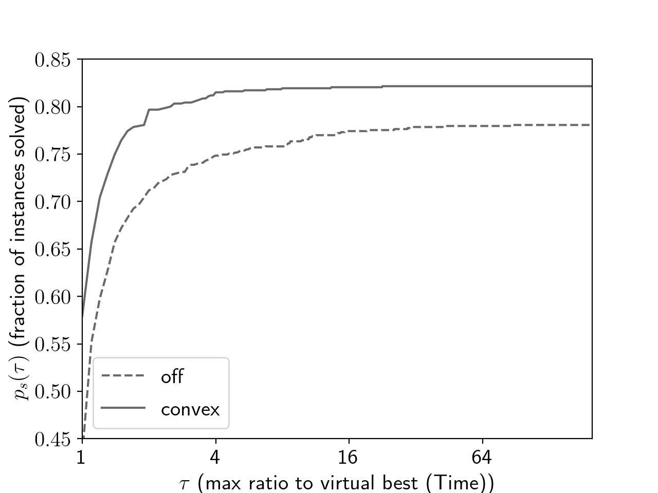
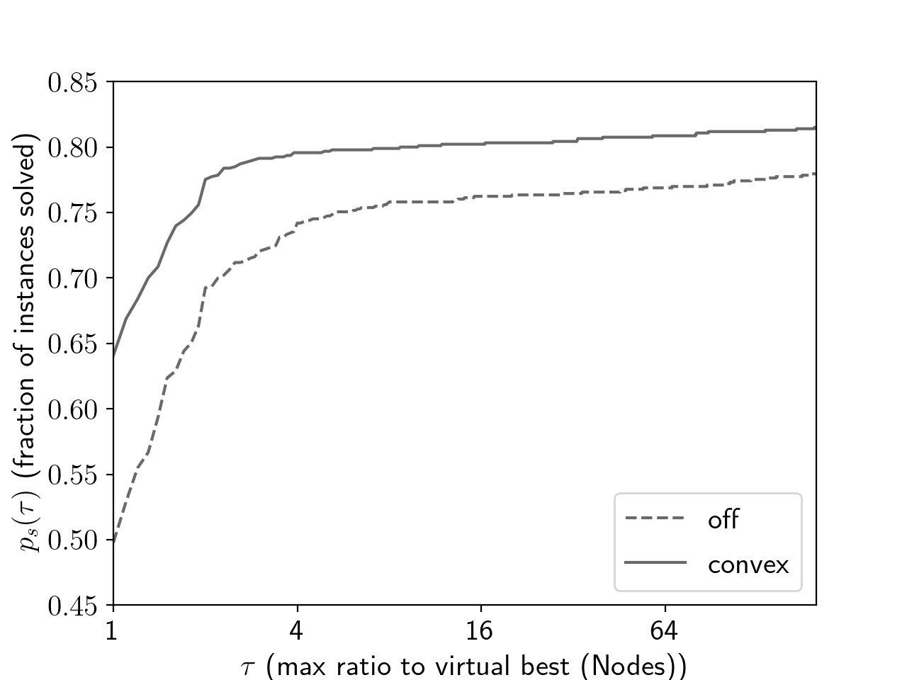
Figure 3: Performance profiles comparing Off and Convex

Figures 3 and 4 show performance profiles [6] for running time and number of nodes with settings Off and Convex and settings Convex and Full, respectively. Let $t_{i,s}$ denote the running time for instance $i$ with setting $s$. The virtual best setting used for the running time performance profiles, denoted by index $vb$, is defined as a setting whose running time for each instance is equal to the minimum of the running times with the two settings that are being compared: $t_{i,vb}=\min_{s}\{t_{i,s}\}$. The horizontal axis represents the maximum allowed ratios to the time with the virtual best setting, denoted by $\tau$. The vertical axis represents the fraction of instances solved within the maximum allowed fraction of time of the virtual best, denoted as $p_{s}(\tau)$:

$$p_{s}(\tau)=\frac{\text{number of instances }i\text{ s.t.: }t_{i,s}\leq\tau\cdot t_{i,vb}}{\text{total number of instances}}.$$

Performance profiles for the number of nodes in the branch-and-bound tree are constructed similarly, the only difference being that $t_{.,.}$ is replaced everywhere with $n_{.,.}$, which represents the number of nodes per instance and setting.

From Figure 3 we see that setting Convex dominates setting Off. With Convex, over 55% of instances are solved faster or as fast as with setting Off. It is able to solve around $80\%$ of instances within a factor of 4 of the best time, and the curve approaches approximately $82\%$ in the limit, i.e., Convex is able to solve around $82\%$ of the instances. The respective numbers for Off lie at around $10\%$ lower than those for Convex. A very similar picture is observed for the number of nodes.

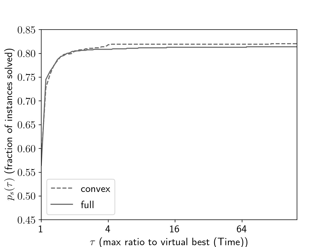
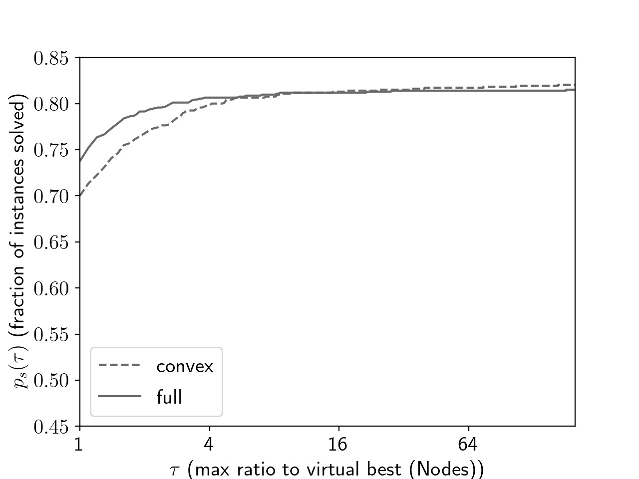
Figure 4: Performance profiles comparing Convex and Full

According to Figure 4, the setting Full is roughly on par with Convex in terms of running time if the ratio we are interested in is below 3. As the ratio increases, Convex becomes the better setting, which reflects the fact that it solves slightly more instances than Full. When looking at the number of nodes, Full yields the best result for around 74% of instances, as opposed to around 70% yielded by Convex. For ratios above 16, Convex is better than Full, which, again, is due to it solving more instances.

5.4 Feature evaluation: bound tightening

As explained in Section 4.3, if the constraint is nonconvex and its relaxation depends on variable bounds, then the indicator variable is first set to 1 and bound tightening is performed. A cut is then computed for this possibly tighter set $F^{1}_{i}$ and strengthened according to Theorem 1. In this subsection we evaluate the usefulness of this feature.

To this end, we introduce the setting Full-noBT. It is equivalent to Full except that the bound tightening feature is disabled. Table 8 compares settings Full-noBT and Full for the 68 affected instances.

Table 8: Comparison between Full-noBT and Full

	Fails	Limit	Solved	RootImpr $>50\%$	Time	Nodes
Full-noBT	16	153	761	4	34.45	2910
Full	17	154	759	25	33.68	2618

When bound tightening is disabled, two more instances are solved due to one less fail and one less time out. Enabling it, on the other hand, leads to large ($>50\%$) root node dual bounds improvements on 25 out of 68 affected instances and a comparable weakening of root node dual bounds only on 4 instances. Enabling bound tightening also yields a small decrease in the mean time ($2.2\%$) and a moderate decrease in the number of nodes ($10\%$). According to these results, the two settings are very close in performance, Full-noBT being the slightly more reliable setting and Full yielding smaller branch-and-bound trees and slightly better solving times.

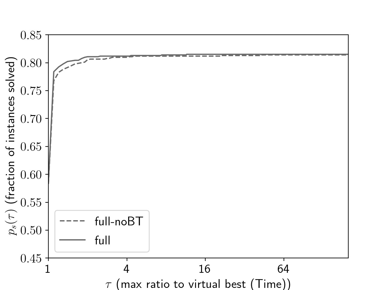
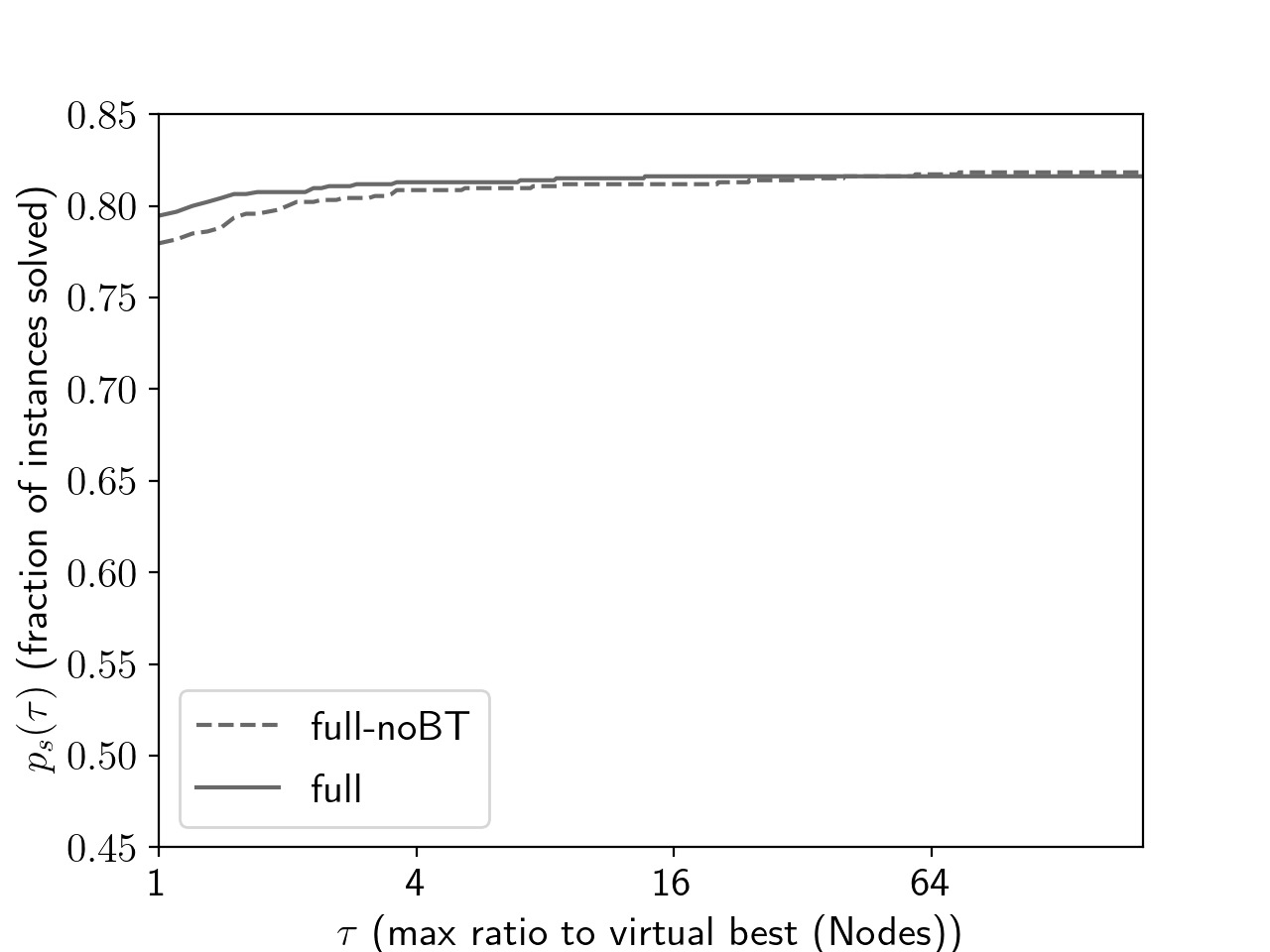
Figure 5: Performance profiles comparing Full-noBT and Full

Performance profiles comparing Full-noBT and Full are shown in Figure 5. The curves are very close since there are few affected instances. The setting Full performed slightly better than Full-noBT both in terms of running times and tree sizes, and the two settings are nearly identical in the limit.

6 Conclusion

In this paper we introduced a general method to construct perspective cuts not only for convex constraints as previously proposed in the literature, but also for nonconvex constraints, for which linear underestimators are readily available. We conducted a computational study of perspective cuts for convex and nonconvex constraints. Relevant structures were detected in about 10% of MINLPLib instances. The computational results indicate that adding perspective cuts for convex constraints reduces the mean running times and tree sizes by over 20%. Adding perspective cuts for nonconvex constraints can be detrimental to performance on challenging instances and can lead to an increased amount of numerical issues, which is reflected in a small decrease in the number of solved instances. Despite this, perspective cuts for nonconvex constraints reduce the geometric mean of the number of nodes of the branch-and-bound tree by 5% and improve dual bounds at the root node.

These results indicate that perspective cuts improve performance of general-purpose solvers. However, in order to efficiently utilize perspective cuts for nonconvex structures, careful implementation and tuning is necessary.

One direction for future work is developing more sophisticated detection algorithms. Some problems contain constraints that do not satisfy the requirements in our current implementation, but with more careful analysis of the problem structure can be revealed to be suitable for applying perspective cuts. Another direction for future research is generalizing the cut strengthening method to on/off variables whose “off” domain is a non-singleton interval, as well as to more general types of on/off sets. Unlike the case considered in this paper, there is no single best choice of how to strengthen a given valid cut in such a setting. Moreover, increased complexity of the set makes developing a computationally efficient cut strengthening method a more challenging task.

Funding

The work for this article has been conducted within the Research Campus MODAL funded by the German Federal Ministry of Education and Research (BMBF grant numbers 05M14ZAM, 05M20ZBM).

The described research activities are funded by the Federal Ministry for Economic Affairs and Energy within the project EnBA-M (ID: 03ET1549D).

References

- [1] Aktürk, M.S., Atamtürk, A., Gürel, S.: A strong conic quadratic reformulation for machine-job assignment with controllable processing times. Operations Research Letters 37(3), 187–191 (2009). doi:10.1016/j.orl.2008.12.009
- [2] Atamtürk, A., Gómez, A.: Strong formulations for quadratic optimization with M-matrices and indicator variables. Mathematical Programming 170(1), 141–176 (2018). doi:10.1007/s10107-018-1301-5
- [3] Barbaro, R., Ramani, R.: Generalized multiperiod MIP model for production scheduling and processing facilities selection and location. Mining Engineering 38(2), 107–114 (1986)
- [4] Bussieck, M.R., Drud, A.S., Meeraus, A.: MINLPLib – a collection of test models for mixed-integer nonlinear programming. INFORMS Journal on Computing 15(1), 114–119 (2003). doi:10.1287/ijoc.15.1.114.15159
- [5] Ceria, S., Soares, J.: Convex programming for disjunctive convex optimization. Mathematical Programming 86(3), 595–614 (1999). doi:10.1007/s101070050106
- [6] Dolan, E.D., Moré, J.J.: Benchmarking optimization software with performance profiles. Mathematical Programming 91(2), 201–213 (2002). doi:10.1007/s101070100263
- [7] Fisher, E.B., O’Neill, R.P., Ferris, M.C.: Optimal transmission switching. IEEE Transactions on Power Systems 23(3), 1346–1355 (2008). doi:10.1109/TPWRS.2008.922256
- [8] Frangioni, A., Furini, F., Gentile, C.: Approximated perspective relaxations: a project and lift approach. Computational Optimization and Applications 63(3), 705–735 (2016). doi:10.1007/s10589-015-9787-8
- [9] Frangioni, A., Gentile, C.: Perspective cuts for a class of convex 0–1 mixed integer programs. Mathematical Programming 106(2), 225–236 (2006). doi:10.1007/s10107-005-0594-3
- [10] Frangioni, A., Gentile, C.: A computational comparison of reformulations of the perspective relaxation: SOCP vs. cutting planes. Operations Research Letters 37(3), 206 – 210 (2009). doi:10.1016/j.orl.2009.02.003
- [11] Frangioni, A., Gentile, C., Grande, E., Pacifici, A.: Projected perspective reformulations with applications in design problems. Operations Research 59(5), 1225–1232 (2011). doi:10.1287/opre.1110.0930
- [12] Gamrath, G., Anderson, D., Bestuzheva, K., Chen, W.K., Eifler, L., Gasse, M., Gemander, P., Gleixner, A., Gottwald, L., Halbig, K., et al.: The SCIP Optimization Suite 7.0. ZIB-Report 20-10, Zuse Institute Berlin (2020)
- [13] Grossmann, I.E., Lee, S.: Generalized convex disjunctive programming: Nonlinear convex hull relaxation. Computational Optimization and Applications 26(1), 83–100 (2003). doi:10.1023/A:1025154322278
- [14] Günlük, O., Linderoth, J.: Perspective reformulations of mixed integer nonlinear programs with indicator variables. Mathematical Programming 124(1-2), 183–205 (2010). doi:10.1007/s10107-010-0360-z
- [15] Günlük, O., Linderoth, J.: Perspective reformulation and applications. In: J. Lee, S. Leyffer (eds.) Mixed Integer Nonlinear Programming, pp. 61–89. Springer, New York, NY (2012). doi:10.1007/978-1-4614-1927-3_3
- [16] Kelley Jr, J.E.: The cutting-plane method for solving convex programs. Journal of the Society for Industrial and Applied Mathematics 8(4), 703–712 (1960). doi:10.1137/0108053
- [17] Lodi, A., Tramontani, A.: Performance variability in mixed-integer programming. In: Theory Driven by Influential Applications, pp. 1–12. INFORMS (2013). doi:10.1287/educ.2013.0112
- [18] Rockafellar, R.T.: Convex analysis. Princeton University Press (2015)
- [19] Salgado, E., Gentile, C., Liberti, L.: Perspective cuts for the ACOPF with generators. In: New Trends in Emerging Complex Real Life Problems, pp. 451–461. Springer (2018)
- [20] Salgado, E., Scozzari, A., Tardella, F., Liberti, L.: Alternating current optimal power flow with generator selection. In: J. Lee, G. Rinaldi, A.R. Mahjoub (eds.) Combinatorial Optimization, pp. 364–375. Springer International Publishing, Cham (2018). doi:10.1007/978-3-319-96151-4_31
- [21] Stubbs, R.A., Mehrotra, S.: A branch-and-cut method for 0-1 mixed convex programming. Mathematical Programming 86(3), 515–532 (1999). doi:10.1007/s101070050103
- [22] Tawarmalani, M., Sahinidis, N.V.: Convex extensions and envelopes of lower semi-continuous functions. Mathematical Programming 93(2), 247–263 (2002). doi:10.1007/s10107-002-0308-z
- [23] Wächter, A., Biegler, L.T.: On the implementation of an interior-point filter line-search algorithm for large-scale nonlinear programming. Mathematical Programming 106(1), 25–57 (2006). doi:10.1007/s10107-004-0559-y
- [24] Williams, H.P.: The reformulation of two mixed integer programming problems. Mathematical Programming 14(1), 325–331 (1978). doi:10.1007/BF01588974