A numerical algorithm based on probing to find optimized transmission conditions

1 Motivation

Optimized Schwarz Methods (OSMs) are very versatile: they can be used with or without overlap, converge faster compared to other domain decomposition methods gander2006optimized , are among the fastest solvers for wave problems gander2019class , and can be robust for heterogeneous problems gander2019heterogeneous . This is due to their general transmission conditions, optimized for the problem at hand. Over the last two decades such conditions have been derived for many Partial Differential Equations (PDEs), see gander2019heterogeneous for a review.

Optimized transmission conditions can be obtained by diagonalizing the OSM iteration using a Fourier transform for two subdomains with a straight interface. This works surprisingly well, but there are important cases where the Fourier approach fails: geometries with curved interfaces (there are studies for specific geometries, e.g. gigante2020optimized ; gander2017optimized ; Gander2014OptimizedSM ), and heterogeneous couplings when the two coupled problems are quite different in terms of eigenvectors of the local Steklov-Poincaré operators gander2018derivation . There is therefore a great need for numerical routines which allow one to get cheaply optimized transmission conditions, which furthermore could then lead to OSM black-box solvers. Our goal is to present one such procedure.

Let us consider the simple case of a two nonoverlapping subdomain decomposition, that is $\Omega=\Omega_{1}\cup\Omega_{2}$, $\Omega_{1}\cap\Omega_{2}=\emptyset$, $\Gamma:=\overline{\Omega_{1}}\cap\overline{\Omega_{2}}$, and a generic second order linear PDE

$$\mathcal{L}(u)=f,\text{ in }\Omega,\quad u=0\text{ on }\partial\Omega.$$ (1)

The operator $\mathcal{L}$ could represent a homogeneous problem, i.e. the same PDE over the whole domain, or it could have discontinuous coefficients along $\Gamma$, or even represent a heterogeneous coupling. Starting from two initial guesses $u_{1}^{0},u_{2}^{0}$, the OSM with double sided zeroth-order transmission conditions computes at iteration $n$

$$\begin{array}[]{r l l l l}\mathcal{L}(u^{n}_{1})&=0&\text{on}\quad\Omega_{1},\quad(\partial_{n_{1}}+s_{1})u^{n}_{1}&=(\partial_{n_{1}}+s_{1})u^{n-1}_{2}&\text{on}\quad\Gamma,\\ \mathcal{L}(u^{n}_{2})&=0&\text{on}\quad\Omega_{2},\quad(\partial_{n_{2}}+s_{2})u^{n}_{2}&=(\partial_{n_{2}}+s_{2})u^{n-1}_{1}&\text{on}\quad\Gamma,\end{array}$$ (2)

where $s_{1},s_{2}\in\mathbb{R}$ are the parameters to optimize.

At the discrete level, the original PDE (1) is equivalent to the linear system

$$\begin{pmatrix}A_{II}^{1}&0&A^{1}_{I\Gamma}\\ 0&A_{II}^{2}&A^{2}_{I\Gamma}\\ A^{1}_{\Gamma I}&A^{2}_{\Gamma I}&A_{\Gamma\Gamma}\end{pmatrix}\begin{pmatrix}\mathbf{u}_{1}\\ \mathbf{u}_{2}\\ \mathbf{u}_{\Gamma}\end{pmatrix}=\begin{pmatrix}\mathbf{f}_{1}\\ \mathbf{f}_{2}\\ \mathbf{f}_{\Gamma}\end{pmatrix},$$

where the unknowns are split into those interior to domain $\Omega_{i}$, that is $\mathbf{u}_{i}$, $i=1,2$, and those lying on the interface $\Gamma$, i.e. $\mathbf{u}_{\Gamma}$. It is well known that the Dirichlet-Neumann and Neumann-Neumann methods can be seen as Richardson type methods to solve the discrete Steklov-Poincaré equation

$$\Sigma\mathbf{u}_{\Gamma}=\mathbf{\mu},$$

where $\Sigma:=\Sigma_{1}+\Sigma_{2}$, $\Sigma_{i}:=A^{i}_{\Gamma\Gamma}-A^{i}_{\Gamma I}(A^{i}_{II})^{-1}A^{i}_{I\Gamma}$, $\mathbf{\mu}:=\mathbf{\mu}_{1}+\mathbf{\mu}_{2}$, $\mathbf{\mu}_{i}:=\mathbf{f}^{i}_{\Gamma}-A^{i}_{\Gamma I}(A^{i}_{II})^{-1}\mathbf{f}_{i}$, $i=1,2$. It is probably less known that the OSM (2) can be interpreted as an Alternating Direction Implicit scheme (ADI, see e.g. axelsson_1994 ), for the solution of the continuous Steklov-Poincaré equation. This interesting point of view has been discussed in agoshkov1990generalized ; discacciati2004domain . At the discrete level, it results in the equivalence between a discretization of (2) and the ADI scheme

$$(s_{1}E+\Sigma_{1})\lambda^{n+\frac{1}{2}}=(s_{1}E-\Sigma_{2})\lambda^{n}+\mu,\quad(s_{2}E+\Sigma_{2})\lambda^{n+1}=(s_{2}E-\Sigma_{1})\lambda^{n+\frac{1}{2}}+\mu,$$

where $E$ is either the mass matrix on $\Gamma$ using a Finite Element discretization, or simply an identity matrix using a Finite Difference stencil. From now on, we will replace $E$ with the identity $I$ without loss of generality. Working on the error equation, the iteration operator of the ADI scheme is

$$T(s_{1},s_{2}):=(s_{2}I+\Sigma_{2})^{-1}(s_{2}I-\Sigma_{1})(s_{1}I+\Sigma_{1})^{-1}(s_{1}I-\Sigma_{2}),$$ (3)

and one would like to minimize the spectral radius, $\min_{s_{1},s_{2}}\rho(T(s_{1},s_{2}))$. It would be natural to use the wide literature available on ADI methods to find the optimized parameters $s_{1},s_{2}$ for OSMs. Unfortunately, the ADI literature contains useful results only in the case where $\Sigma_{1}$ and $\Sigma_{2}$ commute, which is quite a strong assumption. In our context, the commutativity holds for instance if $\Omega_{1}=\Omega_{2}$ and $\mathcal{L}$ represents a homogeneous PDE. Under these hypotheses, Fourier analysis already provides good estimates of the optimized parameters. Indeed it can be shown quite generally that the Fourier analysis and ADI theory lead to the same estimates. Without the commutativity assumption, the ADI theory relies on rough upper bounds which do not lead to precise estimates of the optimized parameters. For more details on the links between ADI methods and OSMs we refer to (vanzan_thesis, , Section 2.5).

Let us observe that if one used more general transmission conditions represented by matrices $\widetilde{\Sigma}_{1}$ and $\widetilde{\Sigma}_{2}$, (3) becomes

$$T(\widetilde{\Sigma}_{1},\widetilde{\Sigma}_{2})=(\widetilde{\Sigma}_{2}+\Sigma_{2})^{-1}(\widetilde{\Sigma}_{2}-\Sigma_{1})(\widetilde{\Sigma}_{1}+\Sigma_{1})^{-1}(\widetilde{\Sigma}_{1}-\Sigma_{2}).$$

Choosing either $\widetilde{\Sigma}_{1}=\Sigma_{2}$ or $\widetilde{\Sigma}_{2}=\Sigma_{1}$ leads to $T=0$, and thus one obtains that the local Steklov-Poincaré operators are optimal transmission operators Nataf .

2 An algorithm based on probing

Our algorithm to find numerically optimized transmission conditions has deep roots in the ADI interpretation of the OSMs and it is based on the probing technique. By probing, we mean the numerical procedure through which we estimate a generic matrix $G$ by testing it over a set of vectors. In mathematical terms, given a set of vectors $\mathbf{x}_{k}$ and $\mathbf{y}_{k}:=G\mathbf{x}_{k}$, $k\in\mathcal{K}$, we consider the problem

$$\text{Find }\widetilde{G}\quad\text{such that}\quad\widetilde{G}\mathbf{x}_{i}=\mathbf{y}_{i},\forall i\in\mathcal{I}.$$ (4)

As we look for matrices with some nice properties ( diagonal, tridiagonal, sparse…), problem (4) does not always have a solution. Calling $D$ the set of admissible matrices, we prefer to consider the problem

$$\min_{\widetilde{G}\in D}\max_{k\in\mathcal{K}}\|\mathbf{y}_{k}-\widetilde{G}\mathbf{x}_{k}\|.$$ (5)

Having remarked that the local Steklov-Poincaré operators represent optimal transmission conditions, it would be natural to approximate them using probing. Unfortunately, this idea turns out to be very inefficient. To see this, let us carry out a continuous analysis on an infinite strip, $\Omega_{1}=(-\infty,0)\times(0,1)$ and $\Omega_{2}=(0,\infty)\times(0,1)$. We consider the Laplace equation and, denoting with $\mathcal{S}_{i}$ the continuous Steklov-Poincaré operators, due to symmetry we have $\mathcal{S}_{1}=\mathcal{S}_{2}=:\mathcal{S}_{e}$. In this simple geometry, the eigenvectors of $\mathcal{S}_{e}$ are $v_{k}=\sin(k\pi y)$, $k\in\mathbb{N}^{+}$ with eigenvalues $\mu_{k}=k\pi$ so that $\mathcal{S}_{e}v_{k}=\mu_{k}v_{k}=:y_{k}$, see gander2006optimized . We look for an operator $S=sI$, $s\in\mathbb{R}^{+}$, which corresponds to a Robin transmission condition with parameter $s$. As probing functions, we choose the normalized functions $v_{k}$, $k=1,...,N_{h}$, where $N_{h}$ is the number of degrees of freedom on the interface. Then (5) becomes

$$\min_{S=sI,\text{ }s\in\mathbb{R}^{+}}\max_{k\in[1,N_{h}]}\|y_{k}-Sv_{k}\|=\min_{s\in\mathbb{R}^{+}}\max_{k\in[1,N_{h}]}\|\mu_{k}v_{k}-sv_{k}\|=\min_{s\in\mathbb{R}^{+}}\max_{k\in[1,N_{h}]}|k\pi-s|.$$ (6)

The solution of (6) is $s^{*}=\frac{N_{h}\pi}{2}$ while, according to a Fourier analysis and numerical evidence gander2006optimized , the optimal parameter is $s^{\text{opt}}=\sqrt{N_{h}\pi}$. This discrepancy is due to the fact that problem (6) aims to make the parenthesis $(s_{i}I-\Sigma_{3-i})$, $i=1,2$ as small as possible, but it completely neglects the other terms $(s_{i}I+\Sigma_{i})$.

This observation suggests to consider the minimization problem

$$\min_{\widetilde{\Sigma}_{1},\widetilde{\Sigma}_{2}\in D}\max_{k\in\mathcal{K}}\textstyle\frac{\|\Sigma_{2}\mathbf{x}_{k}-\widetilde{\Sigma}_{1}\mathbf{x}_{k}\|}{\|\Sigma_{1}\mathbf{x}_{k}+\widetilde{\Sigma}_{1}\mathbf{x}_{k}\|}\frac{\|\Sigma_{1}\mathbf{x}_{k}-\widetilde{\Sigma}_{2}\mathbf{x}_{k}\|}{\|\Sigma_{2}\mathbf{x}_{k}+\widetilde{\Sigma}_{2}\mathbf{x}_{k}\|}.$$ (7)

We say that this problem is consistent in the sense that, assuming $\Sigma_{1},\Sigma_{2}$ share a common eigenbasis $\left\{\mathbf{v}_{k}\right\}_{k}$ with eigenvalues $\left\{\mu_{k}^{i}\right\}$, $\widetilde{\Sigma}_{i}=s_{i}I$, $i=1,2$, $k=1,\dots,N_{h}$, then choosing $\mathbf{x}_{k}=\mathbf{v}_{k}$, we have

$$\min_{\widetilde{\Sigma}_{1},\widetilde{\Sigma}_{2}\in D}\max_{k\in\mathcal{K}}\textstyle\frac{\|\Sigma_{2}\mathbf{x}_{k}-\widetilde{\Sigma}_{1}\mathbf{x}_{k}\|}{\|\Sigma_{1}\mathbf{x}_{k}+\widetilde{\Sigma}_{1}\mathbf{x}_{k}\|}\frac{\|\Sigma_{1}\mathbf{x}_{k}-\widetilde{\Sigma}_{2}\mathbf{x}_{k}\|}{\|\Sigma_{2}\mathbf{x}_{k}+\widetilde{\Sigma}_{2}\mathbf{x}_{k}\|}=\min_{s_{1},s_{2}}\max_{k\in\mathcal{I}}\in\textstyle\left|\frac{s_{1}-\mu^{2}_{k}}{s_{1}+\mu^{1}_{k}}\frac{s_{2}-\mu^{1}_{k}}{s_{2}+\mu^{2}_{k}}\right|=\min_{s_{1},s_{2}\in\mathbb{R}^{+}}\rho(T(s_{1},s_{2})),$$

that is, (7) is equivalent to minimize the spectral radius of the iteration matrix.

We thus propose our numerical procedure to find optimized transmission conditions, summarized in Steps 2-4 of Algorithm 1.

0:  A set of vector $\mathbf{x}_{k}$, $k\in\mathcal{K}$, a characterization of $\widetilde{\Sigma}_{1}$, $\widetilde{\Sigma}_{2}$.

1:  [Optional] For $i=1,2$, perform $N$ iterations of the power method to get approximations of selected eigenvectors $\mathbf{x}^{i}_{k}$, $i=1,2$, $k\in\mathcal{K}$. Map $\mathbf{x}^{i}_{j}$ into $\mathbf{x}_{k}$, for $i=1,2$, $j\in\mathcal{K}$ and $k=1,\dots,2|\mathcal{K}|$. Redefine $\mathcal{K}:=\left\{1,\dots,2|\mathcal{K}|\right\}$.

2:  Compute $y^{i}_{k}=\Sigma_{i}\mathbf{x}_{k},k\in\mathcal{K}$,.

3:  Call an optimization routine to solve (7).

4:  Return the matrices $\widetilde{\Sigma}_{j}$, $j=1,2$.

Algorithm 1

It requires as input a set of probing vectors and a characterization for the transmission matrices $\widetilde{\Sigma}_{i}$, that is if the matrices are identity times a real parameter, diagonal, or tridiagonal, sparse etc. We then precompute the action of the local Schur complement on the probing vectors. We finally solve (7) using an optimization routine such as fminsearch in Matlab, which is based on the Nelder-Mead algorithm.

The application of $\Sigma_{i}$ to a vector $\mathbf{x}_{k}$ requires a subdomain solve, thus Step 2 requires $2|\mathcal{K}|$ subdomain solves which are embarrassingly parallel. Step 3 does not require any subdomain solves, and thus is not expensive.

As discussed in Section 3, the choice of probing vectors plays a key role to obtain good estimates. Due to the extensive theoretical literature available, the probing vectors should be heuristically related to the eigenvectors associated to the minimum and maximum eigenvalues of $\Sigma_{i}$. It is possible to set the probing vectors $\mathbf{x}_{k}$ equal to lowest and highest Fourier modes. This approach is efficient when the Fourier analysis itself would provide relatively good approximations of the parameters. However there are instances, e.g. curved interfaces or heterogeneous problems, where it is preferable to have problem-dependent probing vectors. We thus include an additional optional step (Step 1), in which, starting from a given set of probing vectors, e.g Fourier modes, we perform $N$ iterations of the power method, which essentially correspond to $N$ iterations of the OSM, to get more suitable problem-dependent probing vectors. To compute the eigenvector associated to the minimum eigenvalue of $\Sigma_{i}$, we rely on the inverse power method which requires to solve a Neumann boundary value problem. Including Step 1, Algorithm 1 requires in total $2|\mathcal{K}|(N+2)$ subdomain solves, where $|\mathcal{K}|$ is the number of probing vectors in the input.

3 Numerical experiments

We start with a sanity check considering a Laplace equation on a rectangle $\Omega$, with $\Omega_{1}=(-1,0)\times(0,1)$, $\Omega_{2}=(0,1)\times(0,1)$ and $\Gamma=\{0\}\times(0,1)$. Given a discretization of the interface $\Gamma$ with $N_{h}$ points, we choose as probing vectors the discretization of

$$x_{1}=\sin(\pi y),\quad x_{2}=\sin(\sqrt{N_{h}}\pi y),\quad x_{3}=\sin(N_{h}\pi y),$$ (8)

motivated by the theoretical analysis in gander2006optimized , which shows that the optimized parameters $s_{i}$ satisfy equioscillation between the minimum, the maximum and a medium frequency which scales as $\sqrt{N_{h}}$. We first look for matrices $\widetilde{\Sigma}_{i}=s_{i}I$ representing zeroth order double sided optimized transmission conditions. Then, we look for matrices $\widehat{\Sigma}_{i}=pI+qH$, where $H$ is a tridiagonal matrix $H:=\text{diag}(\frac{2}{h^{2}})-\text{diag}(\frac{1}{h^{2}},-1)-\text{diag}(\frac{1}{h^{2}},+1)$, where $h$ is the mesh size. At the continuous level, $\widehat{\Sigma}_{i}$ represent second order transmission conditions. Fig. 1 shows that Alg. 1 permits to obtain excellent estimates in both cases with just three probing vectors.

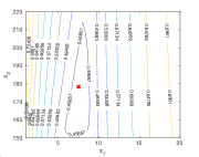
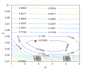
Figure 1: Contour plot of the spectral radius of the iteration matrix $T(\widetilde{\Sigma}_{1},\widetilde{\Sigma}_{2})$ with $\widetilde{\Sigma}_{i}=s_{i}I$ (left) and of $T(\widehat{\Sigma}_{1},\widehat{\Sigma}_{2})$ with $\widehat{\Sigma}_{i}=pI+qH$ (right). The red crosses are the parameters obtained through Alg. 1.

We emphasize that Alg. 1 requires 6 subdomain solves, which can be done in parallel, and leads to a convergence factor of order $\approx 0.07$ for second order transmission conditions. It is clear that, depending on the problem at hand, this addition of 6 subdomain solves is negligible, considering the advantage of having such a small convergence factor.

We now look at a more challenging problem. We solve a second order PDE

$$-\nabla\cdot\nu(\mathbf{x})\nabla u+\mathbf{a}(\mathbf{x})^{\top}\cdot\nabla u+\eta(\mathbf{x})u=f\quad\text{in }\Omega,$$ (9)

where $\Omega$ is represented in Fig. 2 on the top-left.

The interface $\Gamma$ is the parametric curve $\gamma(t):[0,1]\rightarrow(r\sin(\widehat{k}\pi t),t)$, with $r\in\mathbb{R}^{+}$. The coefficients are set to $\nu(\mathbf{x})=1$, $\mathbf{a}(\mathbf{x})=(10(y+x^{2}),0)^{\top}$, $\eta(\mathbf{x})=0.1(x^{2}+y^{2})$ in $\Omega_{1}$, $\nu(\mathbf{x})=100$, $\mathbf{a}(\mathbf{x})=(10(1-x),x)^{\top}$, $\eta(\mathbf{x})=0$ in $\Omega_{2}$, $f(\mathbf{x})=x^{2}+y^{2}$ in $\Omega$. The geometric parameters are $r=0.4$, $\widehat{k}=6$ and the interface is discretized with $N_{h}=100$ points. Driven by the theoretical analysis gander2019heterogeneous , we rescale the transmission conditions according to the physical parameters, setting $S_{i}:=f_{i}(s)I$, where $f_{i}:=\nu_{i}(s^{2}+\frac{a_{i1}^{2}}{4\nu_{i}^{2}}+\frac{a_{i2}^{2}}{4\nu_{i}^{2}}+\frac{\eta_{i}}{\nu_{i}})^{1/2}-\frac{a_{i1}}{2}$. The left panel of Fig. 2 shows a comparison of the optimized parameters obtained by a Fourier analysis to the one obtained by Alg. 1 using as probing vectors the sine frequencies (8). It is evident that both do not deliver efficient estimates. The failure of Alg. 1 is due to the fact that, in contrast to the Laplace case, the sine frequencies do not contain information about the slowest modes. On the right panel of Fig 2, we plot the lowest eigenvectors of $\Sigma_{i}$, which clearly differ significantly from the simple lowest sine frequency. We therefore consider Alg. 1 with the optional Step 1 and as starting probing vectors we only use the lowest and highest sine frequencies. The left panel of Fig. 2 shows that Alg. 1 delivers efficient estimates with just one iteration of the power method.

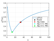
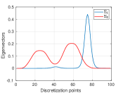
Figure 2: Left: $\Omega$ decomposed into $\Omega_{1}$ and $\Omega_{2}$. Middle: optimized parameters obtained using Fourier analysis or Algorithm 1 with different sets of probing vectors. Right: eigenvectors associated to the smallest eigenvalues of $\Sigma_{j}$, $j=1,2$.

Let us now study the computational cost. To solve (9) up to a tolerance of $10^{-8}$ on the error, an OSM using the Fourier estimated parameters (black cross in Fig 2) requires 21 iterations, while only 12 are needed by Algorithm 1 with only one iteration of the power method. In the offline phase of Algorithm 1, we need to solve $4$ subdomain problems in parallel in Step 1, and further $8$ subdomain problems again in parallel in Step 2. Therefore the cost of the offline phase is equivalent to two iterations of the OSM in a parallel implementation, and consequently Alg. 1 is computationally attractive even in a single-query context.

Fourier estimates depend on the choice of $k_{\min}$ and $k_{\max}$ and in Fig. 2, we set $k_{\min}=\pi$ and $k_{\max}=\pi/h$. Inspired by Gander2014OptimizedSM and a reviewer’s comment, we optimized with $k_{\min}=\pi/|\Gamma|\approx\pi/4.96$ obtaining $s=14.41$, which is very close to the optimal $s^{*}$. However, rescaling $k_{\min}$ with $|\Gamma|$ is not generally a valid approach. Considering $\Omega_{1}$ as the ellipse of boundary $(\cos(2\pi t),0.5\sin(2\pi t))$, $t\in(0,1)$, and $\Omega_{2}=[0,2]\times[0,1]\setminus\Omega_{1}$, see Fig. 2 bottom-left, then $s^{*}=40$, while $s_{k_{\min}=\pi}=31.5$ and $s_{k_{\min}=\pi/|\Gamma|}=20.44$. Thus, rescaling $k_{\min}$ worsens the Fourier estimate.

Next, we consider the Stokes-Darcy system in $\Omega$, with $\Omega_{1}=(-1,0)\times(0,1)$, $\Omega_{2}=(0,1)\times(0,1)$ and $\Gamma=\{0\}\times(0,1)$ with homogeneous Dirichlet boundary conditions along $\partial\Omega$. Refs. gander2018derivation ; vanzan_thesis show that the Fourier analysis fails to provide optimized parameters since the two subproblems do not share a common separation of variable expansion in bounded domains, unless periodic boundary conditions are enforced, see also gander2019heterogeneous [Section 3.3]. Thus, the sine functions do not diagonalize the OSM iteration, even in the simplified domain $\Omega$ with straight interface. Nevertheless, we apply Alg. 1 using two different sets of sines as probing vectors, corresponding to frequencies $\mathcal{K}_{1}=\left\{1,\sqrt{N_{h}},N_{h}\right\}$ and $\mathcal{K}_{2}=\left\{1,2,\sqrt{N_{h}},N_{h}\right\}$. In $\mathcal{K}_{2}$ the first even frequency is included because in Ref. gander2018derivation it was observed that the first odd Fourier frequency converges extremely fast.

Fig 3 shows the estimated parameters for single and double sided zeroth order transmission conditions obtained through a Fourier analysis discacciati2018optimized and using Alg. 1. The left panel confirms the intuition of gander2018derivation , that is, the first even frequency plays a key role in the convergence. The right panel shows that Alg. 1, either with $\mathcal{K}_{1}$ or $\mathcal{K}_{2}$ provides better optimized parameters than the Fourier approach.

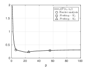
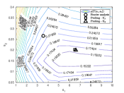
Figure 3: Comparison between the optimized parameters obtained through Fourier analysis and Alg. 1 for single sided Robin boundary conditions (left) and double sided Robin boundary conditions (right).

Next, we consider the stationary heat transfer model coupling the diffusion equation $\nabla\cdot\left(-\lambda\nabla u_{1}(\mathbf{x})\right)=0$ in the porous medium domain $\Omega_{1}=(0,L)\times(5,15)$ with the convection diffusion equation $\nabla\cdot\left(u_{2}(\mathbf{x}){\bf V}_{t}(y)-\lambda_{t}(y)\nabla u_{2}(\mathbf{x})\right)=0$ in the free flow domain $\Omega_{2}=(0,L)\times(0,5)$. Both the turbulent velocity ${\bf V}_{t}=(V_{t}(y),0)^{T}$ and the thermal conductivity $\lambda_{t}(y)$ exhibit a boundary layer at the interface $\Gamma=(0,L)\times\{5\}$ and are computed from the Dittus-Boelter turbulent model. Dirichlet boundary conditions are prescribed at the top of $\Omega_{1}$ and on the left of $\Omega_{2}$, homogeneous Neumann boundary conditions are set on the left and right of $\Omega_{1}$ and at the bottom of $\Omega_{2}$, and a zero Fourier flux is imposed on the right of $\Omega_{2}$. Flux and temperature continuity is imposed at the interface $\Gamma$. The model is discretized by a Finite Volume scheme on a Cartesian mesh of size $50\times 143$ refined on both sides of the interface. Figure 4

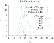
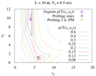
Figure 4: For $L=100$ m, $\overline{V}_{t}=5$ m/s (left) and $L=10$ m, $\overline{V}_{t}=0.5$ m/s (right), comparison of the double sided Robin parameters $s_{1}$ and $s_{2}$ obtained from the probing algorithm using either the 3 sine vectors or the 6 vectors obtained from the 3 sines vectors by 2 PM iterations on both sides. It is compared with the minimizer of the spectral radius $\rho(T(s_{1},s_{2}))$.

shows that the probing algorithm provides a very good approximation of the optimal solution for the case $L=100$ m, $\overline{V}_{t}=5$ m/s (mean velocity) both with the 3 sine vectors (8) and with the 6 vectors obtained from the power method starting from the sine vectors. In the case $L=10$ m, $\overline{V}_{t}=0.5$ m/s, the spectral radius has a narrow valley with two minima. In that case the probing algorithm fails to find the best local minimum but still provides a very efficient approximation.

References

- (1) Agoshkov, V., Lebedev, V.: Generalized Schwarz algorithm with variable parameters. Russian J. Num. Anal. and Math. Model. 5(1), 1–26 (1990)
- (2) Axelsson, O.: Iterative Solution Methods. Cambridge University Press (1994)
- (3) Discacciati, M.: Domain decomposition methods for the coupling of surface and groundwater flows. Ph.D. thesis, Ecole Polytecnique Fédérale de Lausanne (2004)
- (4) Discacciati, M., Gerardo-Giorda, L.: Optimized schwarz methods for the stokes–darcy coupling. IMA J. Num. Anal. 38(4), 1959–1983 (2018)
- (5) Gander, M.J.: Optimized Schwarz methods. SIAM J. Num. Anal. 44(2), 699–731 (2006)
- (6) Gander, M.J., Vanzan, T.: On the derivation of optimized transmission conditions for the Stokes-Darcy coupling. In: International Conference on Domain Decomposition Methods, pp. 491–498. Springer (2018)
- (7) Gander, M.J., Vanzan, T.: Heterogeneous optimized Schwarz methods for second order elliptic PDEs. SIAM J. Sci. Comput. 41(4), A2329–A2354 (2019)
- (8) Gander, M.J., Xu, Y.: Optimized Schwarz methods for circular domain decompositions with overlap. SIAM J. Numer. Anal. 52, 1981–2004 (2014)
- (9) Gander, M.J., Xu, Y.: Optimized Schwarz methods for domain decompositions with parabolic interfaces. In: Domain Decomposition Methods in Science and Engineering XXIII, pp. 323–331. Springer (2017)
- (10) Gander, M.J., Zhang, H.: A class of iterative solvers for the Helmholtz equation: Factorizations, sweeping preconditioners, source transfer, single layer potentials, polarized traces, and optimized Schwarz methods. SIAM Review 61(1), 3–76 (2019)
- (11) Gigante, G., Sambataro, G., Vergara, C.: Optimized Schwarz methods for spherical interfaces with application to fluid-structure interaction. SIAM J. Sci. Comput. 42(2), A751–A770 (2020)
- (12) Nataf, F., Rogier, F., De Sturler, E.: Optimal interface conditions for domain decomposition methods. Tech. rep., École Polytechnique de Paris (1994)
- (13) Vanzan, T.: Domain decomposition methods for multiphysics problems. Ph.D. thesis, Université de Genève (2020)