The power spectrum and structure function of the Gamma Ray emission from the Large Magellanic Cloud

Abstract

The Fermi-LAT observational data of the diffuse $\gamma$ ray emission from the Large Magellanic Cloud (LMC), were examined to test for the existence of underlying long range correlations. A statistical test applied to the data indicated that the probability that data are random is $\sim 10^{-99}$. Thus we proceeded and have used the counts-number data to compute 2D spatial autocorrelation, power spectrum, and structure function.

The most important result of the present study is a clear indication for large scale spatial underlying correlations. This is evident in all the functions mentioned above. The 2D power spectrum has a logarithmic slope of -3 on large spatial scales and a logarithmic slope of -4 on small spatial scales. The structure function has logarithmic slopes equaling 1 and 2 for the large and small scales respectively. The logarithmic slopes of the structure function and the power spectrum are consistent.

A plausible interpretation of these results is the existence of a large scale compressible turbulence with a 3D logarithmic slope of -4 extending over the entire extent of the LMC. This may reflect the fact that the $\gamma$ Ray emission is in star forming regions, where jets and shocks are abundant. Both the power spectrum and structure function exhibit steeper logarithmic slopes for smaller spatial scales. This is interpreted as an indication that the turbulent region has an effective depth of about 1.5 kpc.

1 Introduction

The Large Magellanic Cloud (LMC) is a satellite galaxy of the Milky Way galaxy. At a distance of $50$ kpc it is close enough to be studied with scrutiny. Indeed detailed observations with different wavelengths were carried out. Interestingly, even the first supernova neutrinos were detected from SN1987A, in the LMC (Hirata et al., 1987; Bionta et al., 1987) .

Spicker & Feitzinger (1988) analyzed the HI data obtained by Rohlfs et al. (1984) whose spatial resolution was $\sim 200$ pc. They have used the data to calculate the autocorrelation structure function of the emission weighted velocity field. They obtained a structure function compatible with turbulence on scales up to 1.5 kpc, which is steeper than the structure function of Kolmogorov turbulence (Kolmogorov, 1941).

Elmegreen et al. (2001) used the the $H_{I}$ emission intensity data of the LMC, obtained by Kim et al. (1998), to compute the spatial power spectrum. The spatial resolution was about 20 pc. They derived a power-law that covered 2 decades of spatial scales in the range of $(20\div 2000)$ pc and seemed consistent with the Kolmogorov turbulence spectrum (Kolmogorov, 1941). The power spectra showed a steepening at a scale of $(100\div 200)$ pc, that was interpreted as the $HI$ disk width. The observations were interpreted as indicating a density turbulence in the ISM of the LMC.

Block et al. (2010) analyzed the LMC infrared Spitzer data (Meixner et al., 2006) and obtained spatial power spectra spanning 3 orders of magnitudes $(7pc\div 7kpc)$ extending over the entire size of the LMC. Here too a steepening at $100\div 200pc$ was observed.

The results of Elmegreen et al. (2001) and Block et al. (2010) suggest the existence of large scale turbulence in the interstellar medium (ISM) of the LMC. In this work we set to find out whether the Fermi-Lat $\gamma Ray$ observations indicate the existence of large scale spatial correlations and if so what is their nature,

In section 2 we address the observational data. In section 3 we present the analysis and we compute the 2D correlation, power spectrum and structure function of the observational data. The interpretation and implications are discussed in section 4. In appendices A and B,we obtain theoretical 2D power spectrum and structure function of data that are the result of integration along the line of sight. These are used to interpret the observational power spectrum and structure function.

2 data

We use the LMC $\gamma$ ray data of the Fermi-Lat collaboration (Ackermann et al., 2016), accumulated over a total observing time span of about 73 months. The region of interest (ROI) of the data covered an angular area of $10^{o}\times 10^{o}$; which considering the inclination corresponds to about $9$ by $9$ kpc. The data given in a FiTS file present the observations after subtraction of a background model (see Ackermann et al. (2016) for details). The pixels are $0.1^{o}\times 0.1^{o}$ in size, namely $90\ pc\times 90\ pc$. The PSF is $0.2^{o}$, which equals two pixels,and the standard deviation at each position is 2 counts per pixel. The data is centered around right ascension $\alpha=80.894^{0}$ and declination $\delta=-69.756^{o}$. The counts are total counts in the range of $0.2-100$ GeV.

Figure 1. displays a 3D plot of the counts per pixel in the ROI, as function of position. The counts peak at the large star forming region Dor30 (Tarntula Nebula).

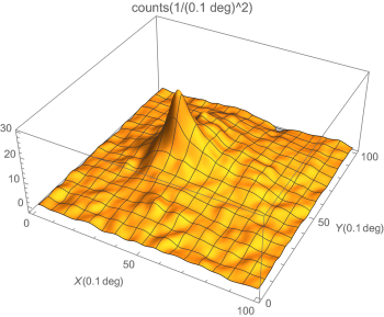
Figure 1: 3D plot of the counts per pixel in the ROI as function of the X (right ascension) and Y(declination) coordinates, in units of 0.1 deg.

3 Analysis

Before starting the data analysis we applied the WolframMathemaica AutoCorrelationTest to the data. This test estimates the probability of the hypothesis that the data are random. The result is a probability $\sim 10^{-99}$ implying that the data are highly auto-correlated.

Figure 2. displays the 2D discrete normalized auto-correlation. The lags are in units of $0.1^{o}$. It is seen that the correlation extends up to the edges of the ROI.

In order to study the nature of this long range spatial correlation we apply two analytical tools: 2D power spectrum and 2D structure function. The power spectrum is especially informative on the smaller spatial scales while structure function complements it by a better covering of the large spatial scales. The structure function has advantage over the power spectrum in treating data at the maps edges (see e.g. Nestingen-Palm et al. (2017)).

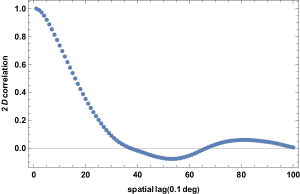
Figure 2: 2D normalized spatial auto-correlation as function of spatial lag, in units of 0.1 deg

3.1 2D power spectrum

We computed the 2D power as function of the 2D wavenumber $k=(k_{x}^{2}+k_{y}^{2})^{1/2}$ by averaging over combinations of $k_{x}$ and $k_{y}$ that yield a given $k$. The discrete FFT was used to compute the Fourier transform.

The 2D power spectrum as function of the dimensionless wave-number $k$ is plotted in figure 3. The units of the power spectrum are $deg^{-4}$, The dimensionless wave number $k$ is defined as $k=\frac{100}{r}$ with $r$ being the dimensionless spatial lag in units of $0.1\ deg$.

The observational power spectrum exhibits a logarithmic slop of $-3$ for the large scales (small $k$) and $-4$ for small scales (large $k$). The logarithmic slope changes at $k\sim 3.5$, which corresponds to a spatial transition scale $r_{t}\sim 2.57\ kpc$. At wave numbers $\gtrsim 17$ corresponding to a scale $\lesssim 0.5$  kpc, the power spectrum steepens considerably.

The error bars were computed by generating simulated data sets that are randomly displaced from the observational values and are within twice the observational standard deviation. For each set the power spectrum was computed, and the standard deviations of the power spectrum were obtained. The error bars in the figures are $2\sigma$.

.

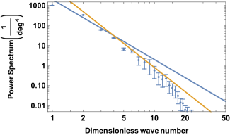
Figure 3: 2D spatial power spectrum. The lines have logarithmic slopes of -3 (blue line) and -4 ( orange line)

3.2 2D structure spectrum

The 2D structure function $S_{2}(r)$ of a 2D quantity $f(x,y)$ is

$$\hskip-19.91684ptS_{2}(r)=<\left(f(x^{\prime},y^{\prime})-f(x^{\prime}+x,y^{\prime}+y)\right)^{2}>$$ (1)

$$~{}=2\bigg{(}C_{2}(0)-C_{2}(r)\bigg{)}\ \ ;\ \ r=\sqrt{x^{2}+y^{2}}$$

where $r$ is the 2D lag between positions. The angular brackets are ensemble average which, by using the ergodic principle, can be replaced by space-average; in this case over the 2D x-y plane.

Figure 4. shows the 2D structure function computed from the data. The structure function shows a transition from a logarithmic slope of 2 for small spatial lags to a slope of 1 for large spatial lags.

.

Figure 4: 2D spatial structure function. The lines have logarithmic slopes of 1(blue line), and 2 ( orange line)

Note that the structure function provides a complimentary description to that of the power spectrum. It provides more points on the larger spatial scales while the power spectrum provides more points on the smaller spatial scales.

The observational transition lag is $r_{t}\sim 1.1^{o}$ corresponding to $\sim 0.99$ kpc.

4 discussion

4.1 The nature of the turbulence

The logarithmic slopes of the observational 2D power spectrum and of the 2D structure function are those expected for a compressible supersonic turbulence. Such turbulent power spectra were observed in HI intensity maps in the Milky Way (MW) galaxy (Green, 1993)and in the SMC (Stanimirovic et al., 1999). This power spectrum has been observed in molecular clouds (Leung et al., 1982), in the HII region Sharpless 142 (Roy & Joncas, 1985), and in numerical simulations (Passot et al., 1988).

The 3D power spectrum is proportional $k{-4}$ with $k$ the absolute value of the 3D wavenumber (and equivalently a 1D power spectrum with logarithmic slope of -2). This is steeper than the Kolmogorov spectrum, which describes subsonic incompressible turbulence with a 1D logarithmic slope of $-5/3$ and a 3D logarithmic slope of $-11/3$.

The steeper slope signals that (unlike in the Kolmogorov spectrum) the rate of energy transferred in the turbulence cascade is not constant but decreases with increasing wavenumber. This is indeed expected in a compressible turbulence since part of the energy at a given wavenumber in the cascade, is diverted to compression of the gas. The existence of this turbulence is in line with observations by Castro et al. (2018) of supersonic $H\alpha$ velocity dispersions of $\sim 40\div 30\ kms^{-1}$ in star forming regions in the LMC.

4.2 The depth of the emitting region

The observed $\gamma$ ray photons originate from different depths along the line of sight. Several authors addressed the issue of power spectra of quantities which are the result of integration along the line-of-sight (Stutzki et al., 1998; Goldman, 2000; Lazarian & Pogosyan, 2000; Miville-Deschênes et al., 2003a). They concluded that when the lateral spatial scale is smaller than the depth of the layer, the logarithmic slope of the power spectrum steepens exactly by $-1$ compared to its value when the lateral scale is large compared to the depth. This behavior was indeed found in as observational power spectra of Galactic and extra Galactic turbulence ( e.g. Elmegreen et al. (2001), Miville-Deschênes et al. (2003b) ) and in solar photospheric turbulence (Abramenko, & Yurchyshyn, 2020).

In Appendix A and Appendix B, we obtain theoretical power spectra and structure function that are the result of integration along the line of sight, For the compressible turbulence we find that the transition from a $-3$ to a $-4$ logarithmic slope occurs at a transition spatial lag $r_{t}=1.67D$ where $D$ is the effective depth from which the the emission originates. The observational value of $r_{t}=2.57$kpc implies a depth $D=1.54$ kpc.

For the structure function we obtained that the transition lag from a logarithmic slope of 1 to a logarithmic slope of $2$ occurs when $r_{SF}=0.63D$. Combining it with observations value obtained in the previous section $r_{SF}=0.99$ kpc, implies a depth $D=1.57$ kpc, in excellent agreement with the value implied by the observational power spectrum.

The effective depth inferred from the power spectrum and structure function is an actual depth. of the turbulent layer because the mean free path of $\gamma$ ray photons turns out to be much larger, as seen below. We note that this depth is an order of magnitude larger than the HI depth obtained by Elmegreen et al. (2001). The large depth traces the depth of star forming regions where the cosmic rays are produced. In this context it is of interest to note that the stellar depth of the LMC, is comparable to its lateral dimensions (Jacyszyn-Dobrzeniecka et al., 2017; Subramanian, & Subramaniam, 2009, 2010). As the lateral dimensions of the star formation regions (notably Dor 30) are $\sim 2$ kpc, the derived depth here makes sense.

4.2.1 The $\gamma$ ray optical depth of the LMC

In order to estimate the optical depth of the $\gamma$ ray photons in the LMC, we use the Klein Nishima cross-section, For photon energies much larger than the rest mass energy of the electron we use (Neronov, 2017).

$$\sigma_{KN}=\frac{3}{8}\sigma_{T}\frac{\ln(2x)}{x}\ \ \ ,\ \ \ x=\frac{E_{\gamma}}{m_{e}c^{2}}$$ (2)

with $\sigma_{T}=6.65\times 10^{-25}\ cm^{2}$ , a typical number density (in star forming regions) of $10^{3}\ {\rm cm^{-3}}$, even the lowest energy photons have mean free path

$$l_{\gamma}\sim 80kpc$$ (3)

This is an order of magnitude larger than the size of the LMC.

4.3 Implication of the observational power spectrum on the cosmic rays spatial distribution

The most likely mechanism for the production of the $\gamma$ rays, adopted also by Ackermann et al. (2016), is that of decay of pions created by energetic cosmic ray (CR) protons scattering off the protons in the LMC interstellar medium. The CR are produced inside the LMC in the star forming regions, notably in 30 Dorados, and confined by the LMC magnetic field. The latter has been investigated by Gaensler et al. (2005) and Mao et al. (2012)who found a mean field along the line of sight of $\sim 1\mu G$ and a disordered field with a coherence length of about $100$ pc and strength of $\sim 10\mu G$. It is conceivable that the weaker mean field is a result of a random walk of the disordered small scale stronger field (Han, 2017).

The cosmic rays are thought to diffuse along the magnetic field lines. The diffusion coefficient is large so that the cosmic ray population tends to be homogeneously spread (Grenier et al., 2015; Krumholz et al., 2020).

The local $\gamma$ ray emissivity is proportional to the product of the number density of the CR and that of the interstellar medium protons. The protons (hydrogen atoms and ions) are those who manifest turbulent fluctuations in velocity and number density. This turbulence is supersonic and is expected to have a 3D power spectrum with logarithmic derivative of -4. The fact that the observational power spectrum is identical to this power spectrum implies that the CR population is indeed homogeneous.

Moreover, since the $\gamma$ ray emission is proportional to the proton number density, it is clear that the $\gamma$ ray production comes practically from the star forming regions where the number density is more than 3 orders of magnitude larger than that in other parts of the ISM.

4.4 Turbulence dissipation scale

As noted in section 3, for $k\gtrsim 17$, corresponding to a spatial scale which is $\lesssim 0.5$ kpc, the power spectrum steepens quite drastically. This may mark the scale below which the microscopic molecular viscosity dissipates the turbulent energy. In what follows, we wish to estimate the expected value of the dissipation scale and compare it with the observational one.

The dissipation scale is defined as the scale below which the microscopic viscosity is larger than the turbulent viscosity, implying that the rate of energy dissipation by the microscopic viscosity exceeds the rate of energy cascaded by the turbulence. Denoting the transition scale by $l_{d}$, and the turbulent kinematic viscosity on this scale, by $\nu_{t}(l_{d})$ one has for the 1D power spectrum which is proportional to $k^{-2}$

$$\nu_{t}(l_{d})\sim\frac{1}{3}V_{t}(l_{d})l_{d}\ ;V_{t}(l_{d})=V_{t}(l_{0})(\frac{l_{d}}{l_{0}})^{0.5}$$ (4)

with $V_{t}(l_{d})$ the turbulent velocity of the dissipation scale, $V_{t}(l_{0})$ is the turbulent velocity on the largest scale $l_{0}=9$ kpc.

The microscopic kinematic viscosity $\nu_{m}$ is

$$\nu_{m}=\frac{1}{3}{c_{s}l_{f}}$$

where $c_{s}$ is the sound speed and $l_{f}$ is the effective mean free path for atoms or ions collisions.

The effective mean free path for the ionized H atoms is the coherence length of the fluctuating magnetic field which is $\sim 100$ pc (Gaensler et al., 2005). The neutral H atoms are coupled to the ionized H atoms on a much smaller scale due to mutual scattering with crossection of $\sim 10^{-16}cm^{2}$.

The two viscosities are equal on the dissipation scale

$$l_{d}=450\ {\rm pc}\left(\frac{c_{s}}{V_{t}(l_{0})}\right)^{2/3}\left(\frac{l_{f}}{100\ {\rm pc}}\right)^{2/3}$$ (5)

This value is indeed consistent with the value suggested by the observational power spectrum.

5 Summary and conclusions

• The main result of the present work is revealing that the LMC $\gamma$ ray intensity exhibits spatial correlations over scales comparable to the size of this galaxy. These correlations manifest via the observational 2D power spectrum and structure function of the $\gamma$ ray intensity. The power spectrum and the structure function are those of compressible supersonic turbulence. The emerging scenario is that of a turbulent ISM and cosmic ray protons which are distributed rather homogeneously. This is consistent with models of cosmic rays diffusion along field lines that suggest such homogeneous distribution..

• The logarithmic slope of the power spectrum changes from $-3$ on large scales to $-4$ on small scales. The logarithmic slope of the structure function changes from $1$ on large scales to $2$ on small scales. This is indeed expected for data which is an integral over the line of sight. Theoretical power spectrum and structure function, detailed in appendix A and appendix B,, were used to infer the depth from the observational power spectrum and structure function. The resulting depth of the emitting region, from both, is $\sim 1.5$ kpc. The large depth reflects the depth of star forming regions where the cosmic rays are produced.

• The large scale of the turbulence requires a generating mechanism which acts on such a global scale. Following Goldman (2000) we suggest that the source generating the turbulence is the tidal interaction with the SMC. The last close passage of the two Magellanic clouds occurred about $200$ MYR ago (Gardiner & Noguchi, 1996; Yoshizawa & Noguchi, 2003) .

  Assuming supersonic turbulent velocity of $\sim 30kms^{-1}$ and largest spatial scale of $\sim 9$ kpc the decay time is $\sim 300$ Myr. Thus the turbulence has not decayed yet. On more local scales of $\sim 1$ kpc there is energy injection from supernovae and jets in the star forming regions.

Appendix A 2D power spectrum of data integrated along the line-of-sight

We are interested in the power spectrum of the counts per unit area in the plane of the sky, $n(\vec{r})$ which is an integral along the line-of -sight $z$ of the counts per unit volume $f(\vec{r},z)$. Here $\vec{r}=(x,y)$ is a position in in the plane of the sky.

$$n(\vec{r})=\int_{0}^{D}f(\vec{r},z)dz$$ (A1)

with $D$ denoting the depth of the turbulence along the line of sight.

The 2-dimensional power spectrum of $n(\vec{r})$ which depends also on $D$ is

$$P_{2}(\vec{k},D)=\int e^{-i\vec{k}\cdot\vec{r}}C_{2}\left(n(\vec{r})\right)d^{2}\vec{r}$$ (A2)

with $C_{2}(\vec{r})$ being the 2D 2-point autocorrelation of the fluctuating $n(\vec{r})$.

$$C_{2}(\vec{r})=<n(\vec{r}^{\prime})n(\vec{r}^{\prime}+\vec{r})>=\int_{0}^{D}\int_{0}^{D}<f(\vec{r}\ ^{\prime},z^{\prime})(f(\vec{r}^{\prime}+\vec{r},z)>dzdz^{\prime}=$$ (A3)

$$\int_{0}^{D}\int_{0}^{D}C_{3}(\vec{r},z-z^{\prime})dzdz^{\prime}=\int_{0}^{D}\int_{0}^{D}P_{3}(\vec{k},k_{z})e^{-i\vec{k}\cdot\vec{r}-ik_{z}(z-z^{\prime})}d^{2}\vec{k}dzdz^{\prime}$$

Here $C_{3}(\vec{r},z-z^{\prime})$ and $P_{3}(\vec{k},k_{z})$ are the 3D autocorrelation and power spectrum, respectively.

From equation (A2) we identify the 2D power spectrum.

$$P_{2}(\vec{k})=\int_{-\infty}^{\infty}\int_{0}^{D}\int_{0}^{D}P_{3}(\vec{k},k_{z})e^{ik_{z}(z-z^{\prime})}dzdz^{\prime}dk_{z}\propto\int_{0}^{\infty}P_{3}(\vec{k},k_{z})\left(\frac{\sin(k_{z}D/2)}{k_{z}D/2}\right)^{2}dk_{z}$$ (A4)

When the 3D power spectrum is a power law and is a function of $k=|{\vec{k}}|$

$$P_{3}(\vec{k},k_{z})\propto(k^{2}+k_{z})^{-(m+2)}$$ (A5)

the 2D power spectrum becomes

$$P_{2}(\vec{k})\propto\int_{0}^{\infty}(k^{2}+k_{z})^{-(m+2)}\left(\frac{\sin(k_{z}D/2)}{k_{z}D/2}\right)^{2}dk_{z}$$ (A6)

For the present case, $m=2$, and using the dimensionless variable $\eta=kD/2$ one gets an analytic solution

$$P_{2}(\eta)\ \propto\eta^{-4}\left(\cosh\eta-\sinh\eta\right)\left(3\eta^{-1}(\eta\cosh\eta-\sinh\eta)+\sinh\eta\right)$$ (A7)

.

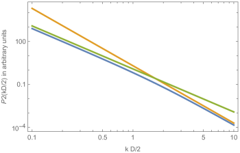
Figure 5: 2D theoretical spatial power spectrum for m=2. The lines have logarithmic slopes of -3 (green line) and -4 (orange line)

Figure 5. displays $P_{2}(kD/2)$. It is seen that for $\eta>>1$ the logarithmic slope is -4 while in the limit $\eta<<1$ the logarithmic slope is -3. A tangent to the curve with a logarithmic slope of $-3.5$ was used (not shown here) to define the transition value of $\eta$ : $\eta_{t}=k_{t}D/2=1.88$ so that $D=3.76/k_{t}=0.6r_{t}$. Here, $k_{t}$ is the transition wave number and $r_{t}=2\pi/k_{t}$ is the transition spatial lag.

Appendix B The 2D structure function of data integrated along the line-of-sight

The 2D correlation is obtained from the 2D power spectrum via

$$C_{2}(\vec{r})=\int_{-\infty}^{\infty}P_{2}(\vec{k})e^{i\vec{k}\cdot\vec{r}}d^{2}\vec{k}$$ (B1)

Using equation (1) and taking note that in the present case, $P_{2}(\vec{k})$ and $C_{2}(\vec{r})$ are functions of the absolute values of $k$, and $r$, respectively, we get

$$S_{2}(r)\propto\int_{0}^{\infty}\sin^{2}(kr/2)\int_{0}^{2\pi}P_{2}(k)e^{ikr\cos\theta}d\theta kdk\propto\int_{0}^{\infty}\sin^{2}(\eta r/D)\int_{0}^{2\pi}P_{2}(\eta)e^{i\eta r/D\cos\theta}d\theta\eta d\eta$$ (B2)

performing the integration over $\theta$, the angle between $\vec{k}$ and $\vec{r}$, yields

$$S_{2}(r)\propto\int_{0}^{\infty}\sin^{2}(\eta r/D)P_{2}(\eta)\pi(1-J_{0}(\eta r/Dr)\ \eta\ d\eta$$ (B3)

$$\propto\int_{0}^{\infty}\sin^{2}(\eta r/D)\eta^{-4}\left(\cosh\eta-\sinh\eta\right)\left(3\eta^{-1}(\eta\cosh\eta-\sinh\eta)+\sinh\eta\right)\eta d\eta$$

Figure 6. displays $S_{2}(r/D)$. It is seen that for $r/D>>1$ the logarithmic slope is 1 while in the limit $r/D<<1$ the logarithmic slope is 2. A tangent to the curve with a logarithmic slope of $1.5$ was used to define the transition value $r_{t}/D=0.63$ implying $D=1.59r_{t}$ with $r_{t}$ denoting the transition spatial scale.

.

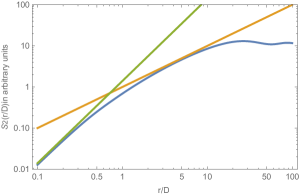
Figure 6: 2D theoretical spatial structure function for m=2. The lines have logarithmic slopes of 1 (orange line ) and 2 (green line)

References

- Abramenko, & Yurchyshyn (2020) Abramenko V. I., Yurchyshyn V. B., 2020, mnras .tmp, doi:10.1093/mnras/staa2427
- Ackermann et al. (2016) Ackermann, M., Albert, A., Atwood, W. B., et al. 2016, A&A, 586, A71.
- Bionta et al. (1987) Bionta, R. M., Blewitt, G., Bratton, C. B., et al. 1987, Phys. Rev. Lett., 58, 1494
- Block et al. (2010) Block, D. L., Puerari, I., Elmegreen, B. G., et al. 2010, ApJ, 718, L1.
- Castro et al. (2018) Castro, N., Crowther, P. A., Evans, C. J., et al. 2018, A&A, 614, A147. doi:10.1051/0004-6361/201732084
- Foreman et al. (2015) Foreman, G., Chu, Y.-H., Gruendl, R., et al. 2015, ApJ, 808, 44
- Elmegreen et al. (2001) Elmegreen, B. G., Kim, S., & Staveley-Smith, L. 2001, ApJ, 548, 749.
- Gaensler et al. (2005) Gaensler, B. M., Haverkorn, M., Staveley-Smith, L., et al. 2005, Science, 307, 1610
- Gardiner & Noguchi (1996) Gardiner, L. T. & Noguchi, M. 1996, MNRAS, 278, 191. doi:10.1093/mnras/278.1.191 S
- Goldman (2000) Goldman, I. 2000, ApJ, 541, 701
- Green (1993) Green, D. A. 1993, MNRAS, 262, 327. doi:10.1093/mnras/262.2.327
- Grenier et al. (2015) Grenier, I. A., Black, J. H., & Strong, A. W. 2015, ARA&A, 53, 199. doi:10.1146/annurev-astro-082214-122457
- Han (2017) Han, J. L. 2017, ARA&A, 55, 111. doi:10.1146/annurev-astro-091916-055221
- Hirata et al. (1987) Hirata, K., Kajita, T., Koshiba, M., et al. 1987, Phys. Rev. Lett., 58, 1490
- Jacyszyn-Dobrzeniecka et al. (2017) Jacyszyn-Dobrzeniecka, A. M., Skowron, D. M., Mróz, P., et al. 2017, Acta Astron., 67, 1.
- Kim et al. (1998) Kim, S., Staveley-Smith, L., Dopita, M. A., et al. 1998, ApJ, 503, 674
- Kolmogorov (1941) Kolmogorov, A. 1941, Akademiia Nauk SSSR Doklady, 30, 301
- Krumholz et al. (2020) Krumholz, M. R., Crocker, R. M., Xu, S., et al. 2020, MNRAS, 493, 2817. doi:10.1093/mnras/staa493
- Lazarian & Pogosyan (2000) Lazarian, A. & Pogosyan, D. 2000, ApJ, 537, 720
- Leung et al. (1982) Leung, C. M., Kutner, M. L., & Mead, K. N. 1982, ApJ, 262, 583. doi:10.1086/160450
- Mao et al. (2012) Mao, S. A., McClure-Griffiths, N. M., Gaensler, B. M., et al. 2012, ApJ, 759, 25.
- Meixner et al. (2006) Meixner, M., Gordon, K. D., Indebetouw, R., et al. 2006, AJ, 132, 2268
- Miville-Deschênes et al. (2003a) Miville-Deschênes, M.-A., Levrier, F., & Falgarone, E. 2003, ApJ, 593, 831
- Miville-Deschênes et al. (2003b) Miville-Deschênes, M.-A., Joncas, G., Falgarone, E., et al. 2003, A&A, 411, 109.
- Neronov (2017) Neronov, A. 2017, lectures, University of Geneva.
- Nestingen-Palm et al. (2017) Nestingen-Palm, D., Stanimirović, S., González-Casanova, D. F., et al. 2017, ApJ, 845, 53.
- Passot et al. (1988) Passot, T., Pouquet, A., & Woodward, P. 1988, A&A, 197, 228
- Rohlfs et al. (1984) Rohlfs, K., Kreitschmann, J., Siegman, B. C., et al. 1984, A&A, 137, 343.
- Roy & Joncas (1985) Roy, J.-R. & Joncas, G. 1985, ApJ, 288, 142. doi:10.1086/162772