Semileptonic form factors of $\Xi_{c}\to\Xi$ in QCD sum rules

Abstract

There exists a significant deviation between the most recent Lattice QCD simulation and experimental measurement by Belle for $\Xi_{c}^{0}\to\Xi^{-}\ell^{+}\nu_{\ell}$. In this work, we investigate the $\Xi_{c}\to\Xi$ form factors in QCD sum rules. To this end, the two-point correlation functions of $\Xi_{c}$ and $\Xi$, and the three-point correlation functions of $\Xi_{c}\to\Xi$ are calculated. At the QCD level, contributions from up to dimension-6 four-quark operators are considered, and the leading order results of the Wilson coefficients are obtained. For the form factors, relatively stable Borel windows can be found. Our form factors are comparable with those of Lattice QCD, except for $f_{\perp}$. The obtained form factors are then used to predict the branching ratios of $\Xi_{c}\to\Xi\ell^{+}\nu_{\ell}$, and our predictions are consistent with the most recent data of ALICE and Belle, and those of Lattice QCD within error. Given that the branching ratios only contain limited information, we suggest the experimentalists directly measure the form factors of $\Xi_{c}\to\Xi$.

I Introduction

Semileptonic decays can be used to extract CKM matrix elements, which are important parameters of the standard model (SM). In addition, lepton flavor universality obtained by studying the semileptonic decays of different leptonic final states is an important tool to test the SM. Recently, Belle reported the measurement of the branching ratios of $\Xi_{c}^{0}\to\Xi^{-}\ell^{+}\nu_{\ell}$ Li:2021uhk :

$${\cal B}(\Xi_{c}^{0}\to\Xi^{-}e^{+}\nu_{e})=(1.31\pm 0.04\pm 0.07\pm 0.38)\%,$$

$${\cal B}(\Xi_{c}^{0}\to\Xi^{-}\mu^{+}\nu_{\mu})=(1.27\pm 0.06\pm 0.10\pm 0.37)\%,$$ (1)

which are already the highest precision for measuring these processes. However, most existing theoretical predictions are more or less larger than these data (see Table 3 below), including various quark model calculations Zhao:2018zcb ; Faustov:2019ddj ; Geng:2020gjh ; Ke:2021pxk , fittings based on SU(3) flavor symmetry Geng:2017mxn ; Geng:2018plk ; Geng:2019bfz , light-cone sum rules (LCSR) analyses Azizi:2011mw ; Aliev:2021wat ; Duan:2022yia . It is particularly worth pointing out that the most recent Lattice QCD simulation in Ref. Zhang:2021oja shows that:

$${\cal B}(\Xi_{c}^{0}\to\Xi^{-}e^{+}\nu_{e})=(2.38\pm 0.30\pm 0.33)\%,$$

$${\cal B}(\Xi_{c}^{0}\to\Xi^{-}\mu^{+}\nu_{\mu})=(2.29\pm 0.29\pm 0.31)\%.$$ (2)

One can see that, there is a significant deviation between experimental measurement and Lattice QCD simulation. Considering the high precision demonstrated by both, this issue deserves further investigation.

The authors of Refs. He:2021qnc ; Geng:2022xfz ; Geng:2022yxb ; Ke:2022gxm suggested that, this tension can be resolved by considering the $\Xi_{c}-\Xi_{c}^{\prime}$ mixing on the theoretical side. However, recent Lattice QCD simulation in Refs. Liu:2023feb ; Liu:2023pwr and QCD sum rules analysis in Ref. Sun:2023noo have shown that this mixing angle is very small, only about $1^{\circ}$. Such a small mixing angle clearly cannot resolve the tension between theory and experiment. The tension still lies there.

A branching ratio itself contains limited information after all. We suggest the experimentalists directly measure the form factors of $\Xi_{c}^{0}\to\Xi^{-}\ell^{+}\nu_{\ell}$, which can be defined as

$$\langle\Xi(p_{2},s_{2})|\bar{s}\gamma_{\mu}(1-\gamma_{5})c|\Xi_{c}(p_{1},s_{1})\rangle$$

$$= \bar{u}(p_{2},s_{2})\left[\gamma_{\mu}f_{1}(q^{2})+i\sigma_{\mu\nu}\frac{q^{\nu}}{M_{1}}f_{2}(q^{2})+\frac{q_{\mu}}{M_{1}}f_{3}(q^{2})\right]u(p_{1},s_{1})$$

$$- \bar{u}(p_{2},s_{2})\left[\gamma_{\mu}g_{1}(q^{2})+i\sigma_{\mu\nu}\frac{q^{\nu}}{M_{1}}g_{2}(q^{2})+\frac{q_{\mu}}{M_{1}}g_{3}(q^{2})\right]\gamma_{5}u(p_{1},s_{1}),$$ (3)

with $M_{1}=m_{\Xi_{c}}$. In fact, BESIII has performed a similar measurement for $\Lambda_{c}^{+}\to\Lambda e^{+}\nu_{e}$ in Ref. BESIII:2022ysa , where the form factors extracted from experiment is directly compared with those obtained from Lattice QCD. The comparison between theory and experiment is sharp and direct, and a very interesting result was found – there exists a significant deviation between experimental measurement and Lattice QCD simulation for the form factors of $\Lambda_{c}^{+}\to\Lambda e^{+}\nu_{e}$. We can say that Ref. BESIII:2022ysa opened an era of fine comparison.

In this work, we will investigate the form factors of $\Xi_{c}\to\Xi$ in QCD sum rules (QCDSR). At the QCD level, contributions from up to dimension-6 four-quark operators are considered; For the Wilson coefficients, the leading order (LO) results are obtained. QCDSR is a QCD-based approach to deal with hadronic parameters. It reveals a direct connection between hadron phenomenology and QCD vacuum structure via a few universal parameters such as quark condensate and gluon condensate. In Refs. Shi:2019hbf ; Xing:2021enr , we systematically applied QCD sum rules for the first time to study the form factors of doubly heavy baryons. To further verify our computing technique, we also investigated the form factors of $\Lambda_{b}\to\Lambda_{c}$, and found that our results were comparable with those of experiment, heavy quark effective theory (HQET) at the next-to-leading power, and Lattice QCD Zhao:2020mod .

The rest of this paper is arranged as follows. In Sec. II, we will investigate the two-point correlation functions of $\Xi_{c}$ and $\Xi$ to obtain their pole residues, which are indispensable inputs when calculating the form factors. At the same time, the continuum threshold parameters, which are the most important parameters in QCDSR in our opinion, are also determined there. In Sec. III, we will outline how to extract the form factors of $\Xi_{c}\to\Xi$ from the three-point correlation functions. Numerical results of form factors and their phenomenological applications will be shown in Sec. IV, where our results are also compared with other theoretical predictions and experimental data. We conclude this paper in the last section.

II Two-point correlation functions and pole residues

To access the $\Xi_{c}\to\Xi$ form factors, the pole residues and continuum threshold parameters of initial and final baryons are indispensable inputs. To this end, in this section we investigate the two-point correlation functions. In the well-known Ref. Ioffe:1981kw , Ioffe, perhaps for the first time, used QCDSR to study the masses of light flavor baryons. In Ref. Yang:1993bp , the authors investigated the neutron-proton mass difference, and contributions from up to dimension-9 operators were included. For the two-point correlation functions of heavy flavor baryons, Wang has already done a lot of work, see, for example, Refs. Wang:2010fq ; Wang:2020mxk . We also analyzed the two-point correlation function of $\Xi_{c}$ in Ref. Zhao:2020mod , but did not consider the contribution of gluon condensate there. For consistency, in this work we recalculate the two-point correlation functions of $\Xi_{c}$ and $\Xi$, with the contribution of gluon condensate being considered.

Sum rules start from the definitions of interpolating currents of hadrons. The following currents are respectively adopted for $\Xi_{c}$ and $\Xi$ Colangelo:2000dp

$$J_{\Xi_{Q}} =\epsilon_{abc}(q_{a}^{T}C\gamma_{5}s_{b})Q_{c},$$

$$J_{\Xi} =\epsilon_{abc}(s_{a}^{T}C\gamma^{\mu}s_{b})\gamma_{\mu}\gamma_{5}q_{c},$$ (4)

where $q$ and $Q$ respectively denote a $u/d$ quark and a charm quark, $a,b,c$ are color indices, and $C$ is the charge conjugation matrix.

The two-point correlation function is defined as

$$\Pi(p)=i\int d^{4}x\ e^{ip\cdot x}\langle 0|T\{J(x)\bar{J}(0)\}|0\rangle.$$ (5)

At the hadron level, after inserting the complete set of hadronic states, the correlation function in Eq. (5) is written into

$$\Pi^{{\rm had}}(p)=\lambda_{+}^{2}\frac{\not{p}+M_{+}}{M_{+}^{2}-p^{2}}+\lambda_{-}^{2}\frac{\not{p}-M_{-}}{M_{-}^{2}-p^{2}}+\cdots,$$ (6)

where the contribution from negative-parity baryon is also considered, and $M_{\pm}$ ($\lambda_{\pm}$) stand for the masses (pole residues) of positive- and negative-parity baryons.

At the QCD level, the correlation function in Eq. (5) can be calculated using OPE technique. In this work, contributions from up to dimension-6 four-quark operators are considered and the corresponding diagrams for $\Xi_{c}$ and $\Xi$ can be found in Fig. 1 and Fig. 2, respectively. The calculation results of the correlation function at the QCD level can be formally written as

$$\Pi^{{\rm QCD}}(p)=A(p^{2})\not{p}+B(p^{2}),$$ (7)

where the coefficient functions $A$ and $B$ can be further written into the following dispersion integrals for practical purpose

$$A(p^{2})=\int ds\ \frac{\rho^{A}(s)}{s-p^{2}},\quad B(p^{2})=\int ds\ \frac{\rho^{B}(s)}{s-p^{2}}.$$ (8)

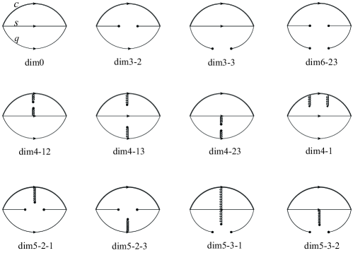
Figure 1: All the diagrams considered for the two-point correlation function of $\Xi_{c}$ at the QCD level.

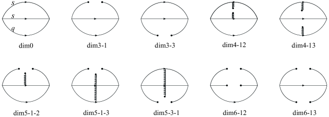
Figure 2: All “independent” diagrams considered for the two-point correlation function of $\Xi$ at the QCD level. Here “independent” means that equivalent diagrams are not shown here.

Taking advantage of quark-hadron duality and then performing the Borel transform, one can arrive at the sum rule for the $1/2^{+}$ baryon

$$(M_{+}+M_{-})\lambda_{+}^{2}\exp(-M_{+}^{2}/T_{+}^{2}) =\int^{s_{+}}ds\ (M_{-}\rho^{A}+\rho^{B})\exp(-s/T_{+}^{2}),$$ (9)

where $T_{+}^{2}$ and $s_{+}$ are the Borel parameter and continuum threshold parameter, respectively. Differentiating Eq. (9) with respect to $-1/T_{+}^{2}$, one can obtain the mass of the $1/2^{+}$ baryon

$$M_{+}^{2}=\frac{\int^{s_{+}}ds\ (M_{-}\rho^{A}+\rho^{B})\ s\ \exp(-s/T_{+}^{2})}{\int^{s_{+}}ds\ (M_{-}\rho^{A}+\rho^{B})\ \exp(-s/T_{+}^{2})}.$$ (10)

In this work, Eq. (10) is viewed as a constraint of Eq. (9), and is used to fix the continuum threshold parameter $s_{+}$, which is the most important parameter in QCDSR in our opinion.

III Three-point correlation functions and form factors

In practice, the following simpler parametrization is adopted to extract the analytical expressions of $\Xi_{c}\to\Xi$ transition form factors:

$$\langle{\cal B}_{2}(p_{2},s_{2})|\bar{s}\gamma_{\mu}(1-\gamma_{5})c|{\cal B}_{1}(p_{1},s_{1})\rangle$$

$$= \bar{u}(p_{2},s_{2})\left[\frac{p_{1\mu}}{M_{1}}F_{1}(q^{2})+\frac{p_{2\mu}}{M_{2}}F_{2}(q^{2})+\gamma_{\mu}F_{3}(q^{2})\right]u(p_{1},s_{1})$$

$$- \bar{u}(p_{2},s_{2})\left[\frac{p_{1\mu}}{M_{1}}G_{1}(q^{2})+\frac{p_{2\mu}}{M_{2}}G_{2}(q^{2})+\gamma_{\mu}G_{3}(q^{2})\right]\gamma_{5}u(p_{1},s_{1}),$$ (11)

where ${\cal B}_{1,2}$ denote $\Xi{}_{c}$ and $\Xi$, respectively. The form factors $F_{i}$ and $G_{i}$ are related to $f_{i}$ and $g_{i}$ defined in Eq. (3) through

$$F_{1}=f_{2}+f_{3},\quad F_{2}=\frac{M_{2}}{M_{1}}(f_{2}-f_{3}),\quad F_{3}=f_{1}-\frac{M_{1}+M_{2}}{M_{1}}f_{2};$$

$$G_{1}=g_{2}+g_{3},\quad G_{2}=\frac{M_{2}}{M_{1}}(g_{2}-g_{3}),\quad G_{3}=g_{1}+\frac{M_{1}-M_{2}}{M_{1}}g_{2}.$$ (12)

In addition, helicity form factors are usually adopted by Lattice QCD Zhang:2021oja ; Detmold:2015aaa , and are related to the form factors in Eq. (3) as follows

$$f_{+}=f_{1}-\frac{q^{2}}{M_{1}(M_{1}+M_{2})}f_{2},\quad f_{\perp}=f_{1}-\frac{M_{1}+M_{2}}{M_{1}}f_{2},\quad f_{0}=f_{1}+\frac{q^{2}}{M_{1}(M_{1}-M_{2})}f_{3},$$

$$g_{+}=g_{1}+\frac{q^{2}}{M_{1}(M_{1}-M_{2})}g_{2},\quad g_{\perp}=g_{1}+\frac{M_{1}-M_{2}}{M_{1}}g_{2},\quad g_{0}=g_{1}-\frac{q^{2}}{M_{1}(M_{1}+M_{2})}g_{3}.$$ (13)

In this work, the results of these helicity form factors are presented to make a close comparison with those of Lattice QCD.

The following three-point correlation functions are defined to extract the form factors of $\Xi_{c}\to\Xi$

$$\Pi_{\mu}^{V,A}(p_{1},p_{2})=i^{2}\int d^{4}xd^{4}y\ e^{-ip_{1}\cdot x+ip_{2}\cdot y}\langle 0|T\{J_{\Xi}(y)(V_{\mu},A_{\mu})(0)\bar{J}_{\Xi_{c}}(x)\}|0\rangle,$$ (14)

where $V_{\mu}(A_{\mu})=\bar{s}\gamma_{\mu}(\gamma_{\mu}\gamma_{5})c$ is the vector (axial-vector) current for the $c\to s$ process. The correlation functions are then calculated at the hadron level and QCD level.

At the hadron level, after inserting the complete sets of initial and final states and considering the contributions from negative-parity baryons, the vector current correlation function in Eq. (14) can be written into

$$\Pi_{\mu}^{V,{\rm had}}(p_{1},p_{2}) = \lambda_{f}^{+}\lambda_{i}^{+}\frac{(\not{p}_{2}+M_{2}^{+})(\frac{p_{1\mu}}{M_{1}^{+}}F_{1}^{++}+\frac{p_{2\mu}}{M_{2}^{+}}F_{2}^{++}+\gamma_{\mu}F_{3}^{++})(\not{p}_{1}+M_{1}^{+})}{(p_{2}^{2}-M_{2}^{+2})(p_{1}^{2}-M_{1}^{+2})}$$ (15)

$$+ \lambda_{f}^{+}\lambda_{i}^{-}\frac{(\not{p}_{2}+M_{2}^{+})(\frac{p_{1\mu}}{M_{1}^{-}}F_{1}^{+-}+\frac{p_{2\mu}}{M_{2}^{+}}F_{2}^{+-}+\gamma_{\mu}F_{3}^{+-})(\not{p}_{1}-M_{1}^{-})}{(p_{2}^{2}-M_{2}^{+2})(p_{1}^{2}-M_{1}^{-2})}$$

$$+ \lambda_{f}^{-}\lambda_{i}^{+}\frac{(\not{p}_{2}-M_{2}^{-})(\frac{p_{1\mu}}{M_{1}^{+}}F_{1}^{-+}+\frac{p_{2\mu}}{M_{2}^{-}}F_{2}^{-+}+\gamma_{\mu}F_{3}^{-+})(\not{p}_{1}+M_{1}^{+})}{(p_{2}^{2}-M_{2}^{-2})(p_{1}^{2}-M_{1}^{+2})}$$

$$+ \lambda_{f}^{-}\lambda_{i}^{-}\frac{(\not{p}_{2}-M_{2}^{-})(\frac{p_{1\mu}}{M_{1}^{-}}F_{1}^{--}+\frac{p_{2\mu}}{M_{2}^{-}}F_{2}^{--}+\gamma_{\mu}F_{3}^{--})(\not{p}_{1}-M_{1}^{-})}{(p_{2}^{2}-M_{2}^{-2})(p_{1}^{2}-M_{1}^{-2})}$$

$$+ \cdots.$$

In Eq. (15), $M_{1(2)}^{+(-)}$ denotes the mass of initial (final) positive- (negative-) parity baryon, and $F_{1}^{+-}$ is the form factor $F_{1}$ with the positive-parity final state and negative-parity initial state, and so forth. To arrive at Eq. (15), we have adopted the following definitions of pole residues for positive- and negative-parity baryons

$$\langle 0|J_{+}|{\cal B}_{+}(p,s)\rangle =\lambda_{+}u(p,s),$$

$$\langle 0|J_{+}|{\cal B}_{-}(p,s)\rangle =(i\gamma_{5})\lambda_{-}u(p,s),$$ (16)

and the following conventions for the 12 form factors $F_{i}^{\pm\pm}$

$$\langle{\cal B}_{f}^{+}(p_{2},s_{2})|V_{\mu}|{\cal B}_{i}^{+}(p_{1},s_{1})\rangle =\bar{u}_{{\cal B}_{f}^{+}}(p_{2},s_{2})[\frac{p_{1\mu}}{M_{1}^{+}}F_{1}^{++}+\frac{p_{2\mu}}{M_{2}^{+}}F_{2}^{++}+\gamma_{\mu}F_{3}^{++}]u_{{\cal B}_{i}^{+}}(p_{1},s_{1}),$$

$$\langle{\cal B}_{f}^{+}(p_{2},s_{2})|V_{\mu}|{\cal B}_{i}^{-}(p_{1},s_{1})\rangle =\bar{u}_{{\cal B}_{f}^{+}}(p_{2},s_{2})[\frac{p_{1\mu}}{M_{1}^{-}}F_{1}^{+-}+\frac{p_{2\mu}}{M_{2}^{+}}F_{2}^{+-}+\gamma_{\mu}F_{3}^{+-}](i\gamma_{5})u_{{\cal B}_{i}^{-}}(p_{1},s_{1}),$$

$$\langle{\cal B}_{f}^{-}(p_{2},s_{2})|V_{\mu}|{\cal B}_{i}^{+}(p_{1},s_{1})\rangle =\bar{u}_{{\cal B}_{f}^{-}}(p_{2},s_{2})(i\gamma_{5})[\frac{p_{1\mu}}{M_{1}^{+}}F_{1}^{-+}+\frac{p_{2\mu}}{M_{2}^{-}}F_{2}^{-+}+\gamma_{\mu}F_{3}^{-+}]u_{{\cal B}_{i}^{+}}(p_{1},s_{1}),$$

$$\langle{\cal B}_{f}^{-}(p_{2},s_{2})|V_{\mu}|{\cal B}_{i}^{-}(p_{1},s_{1})\rangle =\bar{u}_{{\cal B}_{f}^{-}}(p_{2},s_{2})(i\gamma_{5})[\frac{p_{1\mu}}{M_{1}^{-}}F_{1}^{--}+\frac{p_{2\mu}}{M_{2}^{-}}F_{2}^{--}+\gamma_{\mu}F_{3}^{--}](i\gamma_{5})u_{{\cal B}_{i}^{-}}(p_{1},s_{1}).$$ (17)

At the QCD level, contributions from up to dimension-6 four-quark operators are considered, as can be seen in Fig. 3. The calculation results of the vector current correlation function in Eq. (14) can be formally written as

$$\Pi_{\mu}^{V,{\rm QCD}}(p_{1},p_{2})=\sum_{i=1}^{12}A_{i}e_{i\mu}$$ (18)

with

$$(e_{1,2,3,4})_{\mu} = \{\not{p}_{2},1\}\times\{p_{1\mu}\}\times\{\not{p}_{1},1\},$$

$$(e_{5,6,7,8})_{\mu} = \{\not{p}_{2},1\}\times\{p_{2\mu}\}\times\{\not{p}_{1},1\},$$

$$(e_{9,10,11,12})_{\mu} = \{\not{p}_{2},1\}\times\{\gamma_{\mu}\}\times\{\not{p}_{1},1\}.$$ (19)

The coefficients $A_{i}$ in Eq. (18) are then expressed as double dispersion integrals

$$A_{i}(p_{1}^{2},p_{2}^{2},q^{2})=\int^{\infty}ds_{1}\int^{\infty}ds_{2}\frac{\rho_{i}(s_{1},s_{2},q^{2})}{(s_{1}-p_{1}^{2})(s_{2}-p_{2}^{2})},$$ (20)

where the spectral functions $\rho_{i}(s_{1},s_{2},q^{2})$ can be obtained by applying Cutkosky cutting rules to the diagrams in Fig. 3.

Equating Eqs. (15) and (18), and using the quark-hadron duality, one can arrive at 12 equations for 12 unknown form factors $F_{i}^{\pm\pm}$. Solving these equations, and then performing the Borel transform, one can obtain the following expressions for $F_{i}^{++}$:

$$\lambda_{i}^{+}\lambda_{f}^{+}(F_{1}^{++}/M_{1}^{+})\exp\left(-\frac{M_{1}^{+2}}{T_{1}^{2}}-\frac{M_{2}^{+2}}{T_{2}^{2}}\right) =\frac{\{M_{1}^{-}M_{2}^{-},M_{2}^{-},M_{1}^{-},1\}.\{{\cal B}A_{1},{\cal B}A_{2},{\cal B}A_{3},{\cal B}A_{4}\}}{(M_{1}^{+}+M_{1}^{-})(M_{2}^{+}+M_{2}^{-})},$$

$$\lambda_{i}^{+}\lambda_{f}^{+}(F_{2}^{++}/M_{2}^{+})\exp\left(-\frac{M_{1}^{+2}}{T_{1}^{2}}-\frac{M_{2}^{+2}}{T_{2}^{2}}\right) =\frac{\{M_{1}^{-}M_{2}^{-},M_{2}^{-},M_{1}^{-},1\}.\{{\cal B}A_{5},{\cal B}A_{6},{\cal B}A_{7},{\cal B}A_{8}\}}{(M_{1}^{+}+M_{1}^{-})(M_{2}^{+}+M_{2}^{-})},$$

$$\lambda_{i}^{+}\lambda_{f}^{+}F_{3}^{++}\exp\left(-\frac{M_{1}^{+2}}{T_{1}^{2}}-\frac{M_{2}^{+2}}{T_{2}^{2}}\right) =\frac{\{M_{1}^{-}M_{2}^{-},M_{2}^{-},M_{1}^{-},1\}.\{{\cal B}A_{9},{\cal B}A_{10},{\cal B}A_{11},{\cal B}A_{12}\}}{(M_{1}^{+}+M_{1}^{-})(M_{2}^{+}+M_{2}^{-})},$$ (21)

where

$${\cal B}A_{i}\equiv\int^{s_{10}}ds_{1}\int^{s_{20}}ds_{2}\ \rho_{i}(s_{1},s_{2},q^{2})\exp(-s_{1}/T_{1}^{2})\exp(-s_{2}/T_{2}^{2}),$$ (22)

are doubly Borel transformed coefficients, with $s_{1(2)}^{0}$ the continuum threshold parameter of the initial (final) baryon, and $T_{1,2}^{2}$ are the Borel parameters.

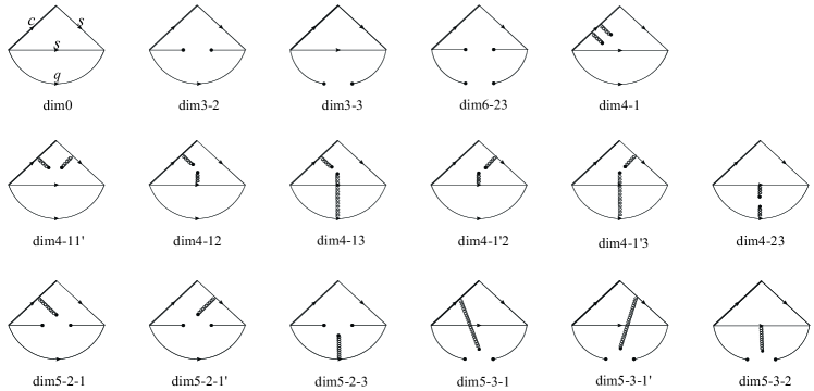
Figure 3: All the diagrams considered for the three-point correlation functions of $\Xi_{c}\to\Xi$ at the QCD level.

III.1 The leading logarithmic corrections

In this work, we also consider the leading logarithmic (LL) corrections for the pole residues and form factors. For this purpose, in the following, we will first briefly summarize some key points of the operator product expansion (OPE) technique.

For two operators ${\cal O}_{1}$ and ${\cal O}_{2}$ separated by a small distance $x$, the product of these two operators can be computed using OPE

$${\cal O}_{1}(x){\cal O}_{2}(0)=\sum_{n}C_{n}(x){\cal O}_{n}(0),$$ (23)

where ${\cal O}_{1,2,n}$ are defined at some renormalizaion scale $\mu$. The calculated Wilson coefficient $C_{n}$ should be multiplied by a LL correction factor Peskin:1995ev

$$\left(\frac{\log(1/|x|^{2}\Lambda_{{\rm QCD}}^{2})}{\log(\mu^{2}/\Lambda_{{\rm QCD}}^{2})}\right)^{(a_{n}-a_{1}-a_{2})/2\beta_{0}},$$ (24)

where $a_{{\cal O}}$ is related to the anomalous dimension $\gamma_{{\cal O}}$ by

$$\gamma_{{\cal O}}=-a_{{\cal O}}\frac{g^{2}}{(4\pi)^{2}},$$ (25)

and $\beta_{0}$ is the first coefficient of the QCD $\beta$ function

$$\beta_{0}=11-\frac{2}{3}n_{f}.$$ (26)

Note that, after performing the Fourier transform as in Eqs. (5) and (14), the inverse of the squared distance $1/|x|^{2}$ is actually $\sim p^{2}$.

In Ref. Zhao:2021xwl , we explicitly calculated the LO anomalous dimensions of the interpolating currents in Eq. (4), and found that the two anomalous dimensions happen to be the same, both equal to

$$\gamma_{J}=-4\frac{g^{2}}{(4\pi)^{2}}.$$ (27)

The anomalous dimension of $\bar{\psi}\psi$ can be found in any standard quantum field theory textbook

$$\gamma_{\bar{\psi}\psi}=-8\frac{g^{2}}{(4\pi)^{2}}.$$ (28)

Following Ioffe in Ref. Ioffe:1981kw , the LL corrections of the Wilson coefficients for higher-dimensional operators are no longer considered due to the following reasons:

• The contribution of these terms is comparatively small.

• The numerical values of higher-dimensional condensate parameters contain large ambiguity.

Some remarks on the OPE of three-point operator product

$${\cal O}_{1}(y){\cal O}_{2}(0){\cal O}_{3}(x)=\sum_{n}C_{n}(x,y){\cal O}_{n}(0)$$ (29)

are in order. If Eq. (29) is considered to have been expanded twice using Eq. (23), one can easily check that in the limit of

$$|x|=|y|,$$ (30)

the corresponding LL correction factor, similar to that in Eq. (24), is

$$\left(\frac{\log(1/|x|^{2}\Lambda_{{\rm QCD}}^{2})}{\log(\mu^{2}/\Lambda_{{\rm QCD}}^{2})}\right)^{(a_{n}-a_{1}-a_{2}-a_{3})/2\beta_{0}}.$$ (31)

For the $B\to\pi$ process, the approximation in Eq. (31) is bad; However, as long as the mass difference between the initial and final states is not very large, this approximation should not be bad. $\Xi_{c}\to\Xi$ can be attributed to the latter situation.

IV Numerical results and phenomenological applications

Numerical results will be shown in this section, and our main results include the pole residues, the continuum threshold parameters of $\Xi_{c}$ and $\Xi$, and the $\Xi_{c}\to\Xi$ form factors. The main inputs include the condensate parameters and quark masses. The condensate parameters are taken as Colangelo:2000dp : $\langle\bar{q}q\rangle(1\ {\rm GeV})=-(0.24\pm 0.01\ {\rm GeV})^{3}$, $\langle\bar{s}s\rangle=(0.8\pm 0.2)\langle\bar{q}q\rangle$, $\langle g_{s}^{2}G^{2}\rangle=(0.47\pm 0.14)\ {\rm GeV}^{4}$, $\langle\bar{q}g_{s}\sigma Gq\rangle=m_{0}^{2}\langle\bar{q}q\rangle$ and $\langle\bar{s}g_{s}\sigma Gs\rangle=m_{0}^{2}\langle\bar{s}s\rangle$ with $m_{0}^{2}=(0.8\pm 0.2)\ {\rm GeV}^{2}$. The following quark masses are adopted ParticleDataGroup:2022pth :

$$m_{c}(m_{c})=1.27\pm 0.02\ {\rm GeV},\quad m_{s}(2\ {\rm GeV})=0.093\pm 0.009\ {\rm GeV},$$ (32)

and $m_{u/d}$ is taken to be 0.

When calculating the pole residues of $\Xi_{c}$ and $\Xi$, and the form factors of $\Xi_{c}\to\Xi$, we take all the renormalization scales at $\mu=m_{c}$. The following equation for the QCD running coupling constant at the one-loop level has been used

$$\alpha_{s}(\mu)=\frac{4\pi}{\beta_{0}\log(\mu^{2}/\Lambda_{{\rm QCD}}^{2})},$$ (33)

and $\alpha_{s}(m_{Z})=0.118$ ParticleDataGroup:2022pth is taken as a reference point for renormalization. The continuity of $\alpha_{s}$ allow to find values of $\Lambda_{{\rm QCD}}^{(n_{f})}$ for different $n_{f}$. It turns out that: $\Lambda_{{\rm QCD}}^{(5)}=88\ {\rm MeV}$, $\Lambda_{{\rm QCD}}^{(4)}=120\ {\rm MeV}$, and $\Lambda_{{\rm QCD}}^{(3)}=143\ {\rm MeV}$. Especially, $\alpha_{s}(m_{c})\approx 0.32$ can be obtained. Then, the quark masses and condensate parameters can be evolved through their respective one-loop evolution formulas. For example, for the quark mass, the one-loop evolution formula is

$$m(\mu_{2})=m(\mu_{1})\left(\frac{\log(\mu_{1}^{2}/\Lambda_{{\rm QCD}}^{2})}{\log(\mu_{2}^{2}/\Lambda_{{\rm QCD}}^{2})}\right)^{4/\beta_{0}}.$$ (34)

As can be seen in Figs. 1, 2, and 3 that, we have only considered the tree-level diagrams – when cutting rules are applied, there is no longer a loop diagram. For the Wilson coefficients, we have only obtained the LO results. As can be seen in our previous work Zhao:2021lzd , the error caused by scale dependence plays an important role. To reduce the dependence of calculation results on the renormalization scale, in this work, we also consider the LL corrections to the Wilson coefficients. However, numerically these corrections are small, the reason is given as follows.

In Eq. (24) and Eq. (31), the renormalization scale $\mu=m_{c}$, and the inverse of the distance $1/|x|$ is exactly or close to ${\cal O}(m_{c})$ for the two-point correlation functions of $\Xi_{c}$ and $\Xi$, and the three-point correlation functions of $\Xi_{c}\to\Xi$. Therefore, all the LL correction factors are all close to $1$, that is, the LL corrections are small (only a few percent).

How to evaluate the contribution from the next-to-leading order (NLO)? This is certainly a difficult question to answer, and often only through detailed calculations at NLO can a clear answer be obtained. The calculation of the decay constants $f_{B_{(s)}}$ in Ref. Jamin:2001fw are excepted to shed some light on the contributions from higher orders. As pointed out in Ref. Jamin:2001fw , in the pole mass scheme, the convergence is poor, while in the $\overline{{\rm MS}}$ scheme, the convergence is good. In the $\overline{{\rm MS}}$ scheme, the contribution from NLO is about 10%. Of course, this is only for the bottom quark case and also limited to the two-point correlation functions. The NLO correction for the charm quark case should be larger.

Inspired by the pole mass scheme, in this work, we also take $m_{c}$ and $m_{s}$ as the pole masses, and expand them to the NLO ParticleDataGroup:2022pth

$$m^{{\rm pole}}=m(\mu)\left(1+\frac{4\alpha_{s}(\mu)}{3\pi}\right)$$ (35)

to evaluate the contribution from NLO. That is, in this work, two sets of results will be presented

• LO + LL + $\overline{{\rm MS}}$ mass, which is taken as the central value;

• LO + LL + pole mass@NLO, which is used to evaluate the contribution from NLO.

We find that, there are respectively about 20%, 15% uncertainties between these two schemes, for the pole residues of $\Xi_{c}$, and the form factors of $\Xi_{c}\to\Xi$. These numbers more or less meet the expectation above. However, it is worth emphasizing again that this is only a very rough estimate, and more accurate numbers can only be known after performing the calculation of NLO.

IV.1 The pole residues of $\Xi_{c}$ and $\Xi$

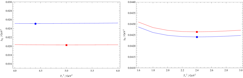
Figure 4: The pole residues of $\Xi_{c}$ and $\Xi$ as functions of the Borel parameter $T_{+}^{2}$. The blue and red curves correspond to the $\overline{{\rm MS}}$ scheme and the pole mass scheme, respectively. The extreme points on these curves correspond to the experimental value of the baryon mass. The $s_{+}$ and $T_{+}^{2}$ corresponding to these extreme points can be found in Table 1.

Table 1: Our predictions of the pole residues of $\Xi_{c}$ and $\Xi$. Optimal $s_{+}$ and $T_{+}^{2}$ are also shown.

$\Xi_{c}$	$(s_{+}/{\rm GeV}^{2},\ T_{+}^{2}/{\rm GeV}^{2})$	$\lambda_{+}/{\rm GeV}^{3}$	$\Xi$	$(s_{+}/{\rm GeV}^{2},\ T_{+}^{2}/{\rm GeV}^{2})$	$\lambda_{+}/{\rm GeV}^{3}$
$\overline{{\rm MS}}$ mass	$(8.74,4.4)$	$0.0251$	$\overline{{\rm MS}}$ mass	$(3.22,2.4)$	$0.0424$
Pole mass@NLO	$(8.70,5.0)$	$0.0203$	Pole mass@NLO	$(3.24,2.4)$	$0.0426$

The pole residues of $\Xi_{c}$ and $\Xi$ are determined using the sum rule in Eq. (9) using Eq. (10) as a constraint, and the corresponding results are shown in Fig. 4 and Table 1. Here is one comment. The experimental masses of $\Xi_{c}^{+,0}$ are respectively $2.468$ GeV and $2.470$ GeV, while those of $\Xi^{0,-}$ are respectively $1.315$ GeV and $1.322$ GeV ParticleDataGroup:2022pth . In Fig. 4 and Table 1, we have actually used the experimental masses of $\Xi_{c}^{0}$ and $\Xi^{-}$. Note that our QCDSR analysis is blind to $u$ or $d$ quark within the hadron.

IV.2 The form factors of $\Xi_{c}\to\Xi$

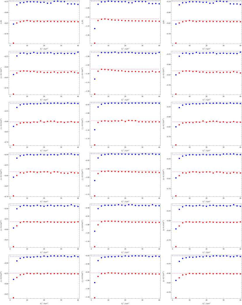
Figure 5: The helicity form factors $f_{+,\perp,0}(q^{2})$ as functions of the Borel parameter $T_{2}^{2}$. The blue dots and red squares respectively correspond to the results obtained using the $\overline{{\rm MS}}$ scheme and the pole mass scheme. $q^{2}=0.0,-0.1,...,-0.5\ {\rm GeV}^{2}$ are considered.

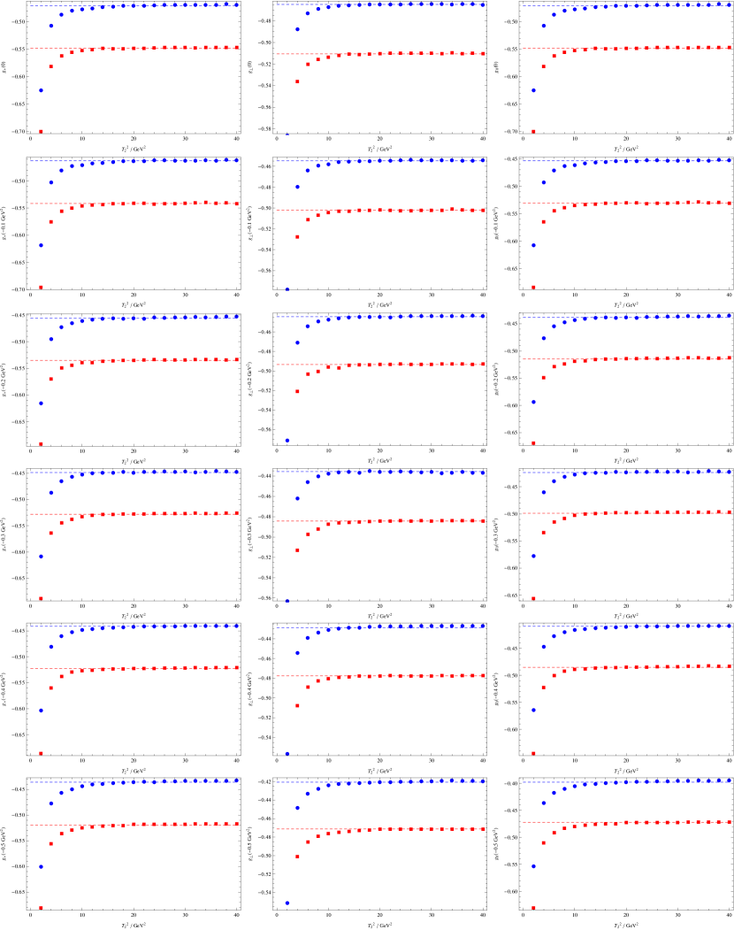
Figure 6: Same as Fig. 5, but for $g_{+,\perp,0}$.

In this subsection, the sum rule in Eq. (21) will be investigated. As the most important parameters in QCDSR, the continuum threshold parameters $s_{1,2}^{0}$ of initial and final states, are taken from corresponding two-point correlation functions, see Table 1.

Reasonable Borel parameters should satisfy $T_{1}^{2}\sim{\cal O}(M_{1}^{2})$ and $T_{2}^{2}\sim{\cal O}(M_{2}^{2})$ with $M_{1,2}$ the masses of initial and final baryons Shifman:1978bx ; Ioffe:1981kw . In the following, we consider a line segment $T_{1}^{2}=3.5\ T_{2}^{2}$ with $T_{2}^{2}\in[2,40]\ {\rm GeV}^{2}$ on the $T_{1}^{2}-T_{2}^{2}$ plane. Relatively stable Borel windows can be found, as can be seen in Figs. 5 and 6.

To access the $q^{2}$ dependence of the $\Xi_{c}\to\Xi$ form factors, we calculate the form factors for $q^{2}\in[-0.5,0]\ {\rm GeV}^{2}$, and then fit the obtained values of $(q^{2},f(q^{2}))$ to the following simplified $z$-expansion:

$$f(q^{2})=\frac{a+b\ z(q^{2})}{1-q^{2}/(m_{{\rm pole}}^{f})^{2}},$$ (36)

where

$$z(q^{2})=\frac{\sqrt{t_{+}-q^{2}}-\sqrt{t_{+}-t_{0}}}{\sqrt{t_{+}-q^{2}}+\sqrt{t_{+}-t_{0}}}$$ (37)

with $t_{+}=(m_{D}+m_{K})^{2}$ and $t_{0}=q_{{\rm max}}^{2}=(m_{\Xi_{c}}-m_{\Xi})^{2}$. The pole masses $m_{{\rm pole}}^{f}$ are respectively taken as $m_{{\rm pole}}^{f_{+},f_{\perp}}=2.112\ {\rm GeV}$, $m_{{\rm pole}}^{f_{0}}=2.318\ {\rm GeV}$, $m_{{\rm pole}}^{g_{+},g_{\perp}}=2.460\ {\rm GeV}$, and $m_{{\rm pole}}^{g_{0}}=1.968\ {\rm GeV}$ Zhang:2021oja . The fitted results of $(a,b)$ are given in Table 2. In Fig. 7, our helicity form factors are compared with those of Lattice QCD Zhang:2021oja . One can see that, most of our form factors are consistent with those of Lattice QCD within error, except for $f_{\perp}$.

Table 2: The fitted results of $(a,b)$ for the $\Xi_{c}\to\Xi$ form factors.

$\overline{{\rm MS}}$ mass	$(a,b)$	Pole mass@NLO	$(a,b)$
$f_{+}$	$(-0.642,1.358)$	$f_{+}$	$(-0.730,1.362)$
$f_{\perp}$	$(-1.208,2.919)$	$f_{\perp}$	$(-1.267,2.329)$
$f_{0}$	$(-0.524,-0.402)$	$f_{0}$	$(-0.585,-0.796)$
$g_{+}$	$(-0.467,-0.050)$	$g_{+}$	$(-0.505,-0.628)$
$g_{\perp}$	$(-0.493,0.433)$	$g_{\perp}$	$(-0.514,0.050)$
$g_{0}$	$(-0.538,1.017)$	$g_{0}$	$(-0.596,0.714)$

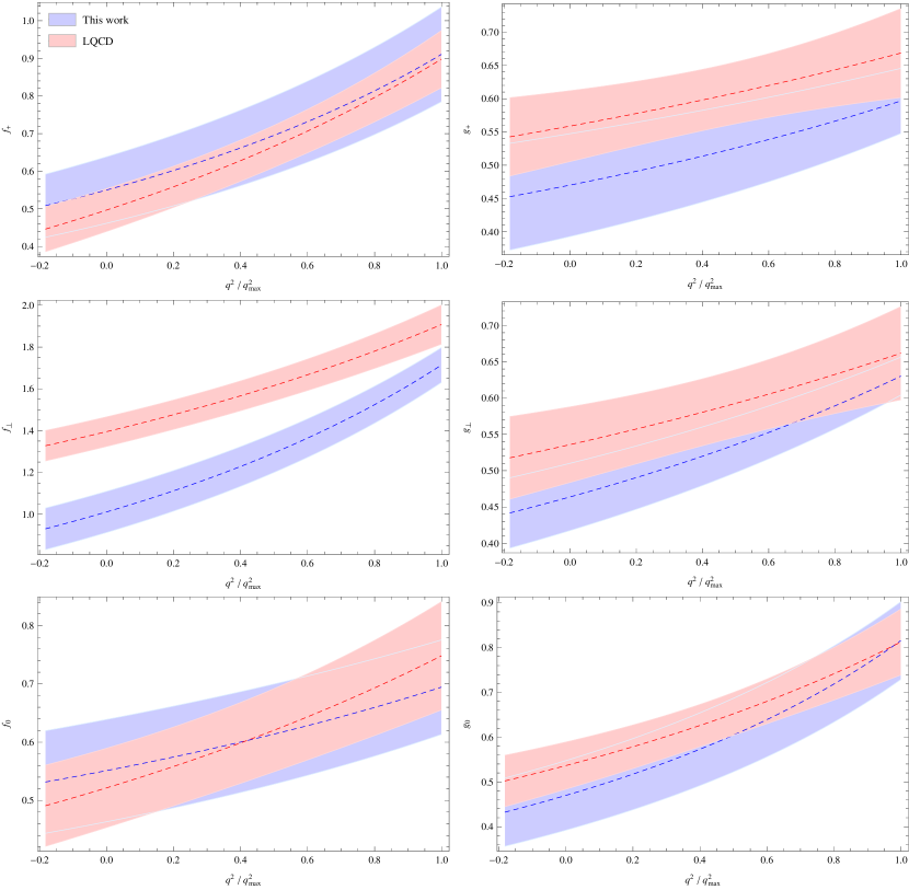
Figure 7: Our helicity form factors are compared with those of Lattice QCD in Ref. Zhang:2021oja . All our form factors have been multiplied by a minus sign.

IV.3 Phenomenological applications

Our form factors are then used to predict the semileptonic decay widths. The polarized decay widths for ${\cal B}_{1}\to{\cal B}_{2}l\nu$ are given by

$$\frac{d\Gamma_{L}}{dq^{2}} =\frac{G_{F}^{2}|V_{{\rm CKM}}|^{2}q^{2}\ p\ (1-\hat{m}_{l}^{2})^{2}}{384\pi^{3}M_{1}^{2}}\left((2+\hat{m}_{l}^{2})(|H_{-\frac{1}{2},0}|^{2}+|H_{\frac{1}{2},0}|^{2})+3\hat{m}_{l}^{2}(|H_{-\frac{1}{2},t}|^{2}+|H_{\frac{1}{2},t}|^{2})\right),$$ (38)

$$\frac{d\Gamma_{T}}{dq^{2}} =\frac{G_{F}^{2}|V_{{\rm CKM}}|^{2}q^{2}\ p\ (1-\hat{m}_{l}^{2})^{2}(2+\hat{m}_{l}^{2})}{384\pi^{3}M_{1}^{2}}(|H_{\frac{1}{2},1}|^{2}+|H_{-\frac{1}{2},-1}|^{2}).$$ (39)

where $\hat{m}_{l}\equiv m_{l}/\sqrt{q^{2}}$, and $p=\sqrt{Q_{+}Q_{-}}/(2M_{1})$ with $Q_{\pm}=(M_{1}\pm M_{2})^{2}-q^{2}$, $M_{1}=m_{\Xi_{c}}$, $M_{2}=m_{\Xi}$. The helicity amplitudes $H_{\lambda_{2},\lambda_{W}}\equiv H_{\lambda_{2},\lambda_{W}}^{V}-H_{\lambda_{2},\lambda_{W}}^{A}$, where $H_{\lambda_{2},\lambda_{W}}^{V,A}$ can be written in terms of the helicity form factors

$$H_{\frac{1}{2},0}^{V}=-i\frac{\sqrt{Q_{-}}}{\sqrt{q^{2}}}(M_{1}+M_{2})f_{+},\quad H_{\frac{1}{2},1}^{V}=-i\sqrt{2Q_{-}}f_{\perp},\quad H_{\frac{1}{2},t}^{V}=-i\frac{\sqrt{Q_{+}}}{\sqrt{q^{2}}}(M_{1}-M_{2})f_{0},$$

$$H_{\frac{1}{2},0}^{A}=-i\frac{\sqrt{Q_{+}}}{\sqrt{q^{2}}}(M_{1}-M_{2})g_{+},\quad H_{\frac{1}{2},1}^{A}=-i\sqrt{2Q_{+}}g_{\perp},\quad H_{\frac{1}{2},t}^{A}=-i\frac{\sqrt{Q_{-}}}{\sqrt{q^{2}}}(M_{1}+M_{2})g_{0},$$ (40)

and

$$H_{-\lambda_{2},-\lambda_{W}}^{V}=H_{\lambda_{2},\lambda_{W}}^{V},\quad H_{-\lambda_{2},-\lambda_{W}}^{A}=-H_{\lambda_{2},\lambda_{W}}^{A}.$$ (41)

Finally, we arrive at:

$${\cal B}(\Xi_{c}^{0}\to\Xi^{-}e^{+}\nu_{e}) =(1.83\pm 0.45)\%,$$

$${\cal B}(\Xi_{c}^{0}\to\Xi^{-}\mu^{+}\nu_{\mu}) =(1.77\pm 0.43)\%,$$

$${\cal B}(\Xi_{c}^{+}\to\Xi^{0}e^{+}\nu_{e}) =(5.58\pm 1.36)\%,$$

$${\cal B}(\Xi_{c}^{+}\to\Xi^{0}\mu^{+}\nu_{\mu}) =(5.38\pm 1.31)\%,$$ (42)

where $\tau(\Xi_{c}^{+})=(453\pm 5)$ fs and $\tau(\Xi_{c}^{0})=(151.9\pm 2.4)$ fs have been used ParticleDataGroup:2022pth . The central values are obtained using the $\overline{{\rm MS}}$ scheme for the quark masses, and the uncertainties are obtained by further considering the pole mass scheme at NLO. One can see from Eq. (42) that, the NLO corrections for the branching ratios may be around $25\%$. In addition, Eq. (42) leads to

$${\cal B}(\Xi_{c}^{0}\to\Xi^{-}e^{+}\nu_{e})/{\cal B}(\Xi_{c}^{0}\to\Xi^{-}\mu^{+}\nu_{\mu})=1.037\pm 0.002,$$ (43)

which is in perfect agreement with the experimental value $1.03\pm 0.05\pm 0.07$ obtained by Belle Li:2021uhk .

Considering the lifetime of $\Xi_{c}^{0}$ changing from around 112 fs in PDG2018 Tanabashi:2018oca to around 152 fs in PDG2022 ParticleDataGroup:2022pth , in Table 3, only the decay width is compared with those from other theoretical predictions and experimental measurements. It can be seen that, most theoretical predictions are larger than the most recent experimental data from Belle, and our result is consistent with those of ALICE and Belle, and that of Lattice QCD.

Table 3: Our decay width of $\Xi_{c}\to\Xi e^{+}\nu_{e}$ (in units of $10^{-13}$ GeV) is compared with experimental data, and other theoretical predictions including Lattice QCD (LQCD), light cone sum rules (LCSR), light-front quark model (LFQM), relativistic quark model (RQM), and SU(3) flavor symmetry (SU(3)).

This work	LCSR Duan:2022yia	LFQM Ke:2021pxk	LCSR Aliev:2021wat	LCSR Azizi:2011mw	SU(3) Geng:2019bfz
$0.79\pm 0.19$	$1.21\pm 0.07$	$0.74\pm 0.15$	$0.80\pm 0.24$	$4.26\pm 1.49$	$1.6\pm 0.1$

RQM Faustov:2019ddj	LFQM Zhao:2018zcb	LQCD Zhang:2021oja	ALICE ALICE	Belle Li:2021uhk
$1.40$	$0.80$	$1.02\pm 0.19$	$1.04\pm 0.36$	$0.563\pm 0.168$

V Conclusions

In this work, the $\Xi_{c}\to\Xi$ form factors are investigated in QCD sum rules. To this end, the two-point correlation functions of $\Xi_{c}$ and $\Xi$, and the three-point correlation functions of $\Xi_{c}\to\Xi$ are calculated. At the QCD level, contributions from up to dimension-6 four-quark operators are considered, and the leading order results of the Wilson coefficients are obtained. As the most important parameters in the calculation of form factors, the continuum threshold parameters of $\Xi_{c}$ and $\Xi$ are determined using the derived sum rule for baryon mass. For the form factors, relatively stable Borel windows can be found. In this sense, our entire calculation has almost no adjustable parameters.

To reduce the scale dependence of our results, the leading logarithmic approximation is considered. To roughly estimate the contribution from the next-to-leading order, we also take the quark masses as the pole masses, and expand them to the next-to-leading order. The corresponding results are then compared with those obtained in the $\overline{{\rm MS}}$ scheme. Finally, our form factors are then used to predict the branching ratios of $\Xi_{c}\to\Xi\ell^{+}\nu_{\ell}$, and we find that the next-to-leading order corrections for the branching ratios may be around $25\%$. Our predictions of the branching ratios are consistent with those of ALICE and Belle, and that of Lattice QCD.

In fact, a branching ratio itself is not enough for precise comparison between theory and experiment. The form factors contain more information! We suggest the experimentalists directly measure the form factors of $\Xi_{c}\to\Xi\ell^{+}\nu_{\ell}$, and we believe that our work will also help resolve the tension between the recent Lattice QCD simulation and Belle’s measurement.

References

(1)
Y. B. Li et al. [Belle],
Phys. Rev. Lett. 127, no.12, 121803 (2021)
doi:10.1103/PhysRevLett.127.121803
[arXiv:2103.06496 [hep-ex]].
(2)
Z. X. Zhao,
Chin. Phys. C 42, no.9, 093101 (2018)
doi:10.1088/1674-1137/42/9/093101
[arXiv:1803.02292 [hep-ph]].
(3)
R. N. Faustov and V. O. Galkin,
Eur. Phys. J. C 79, no.8, 695 (2019)
doi:10.1140/epjc/s10052-019-7214-5
[arXiv:1905.08652 [hep-ph]].
(4)
C. Q. Geng, C. W. Liu and T. H. Tsai,
Phys. Rev. D 103, no.5, 054018 (2021)
doi:10.1103/PhysRevD.103.054018
[arXiv:2012.04147 [hep-ph]].
(5)
H. W. Ke, Q. Q. Kang, X. H. Liu and X. Q. Li,
Chin. Phys. C 45, no.11, 113103 (2021)
doi:10.1088/1674-1137/ac1c66
[arXiv:2106.07013 [hep-ph]].
(6)
C. Q. Geng, Y. K. Hsiao, C. W. Liu and T. H. Tsai,
JHEP 11, 147 (2017)
doi:10.1007/JHEP11(2017)147
[arXiv:1709.00808 [hep-ph]].
(7)
C. Q. Geng, Y. K. Hsiao, C. W. Liu and T. H. Tsai,
Phys. Rev. D 97, no.7, 073006 (2018)
doi:10.1103/PhysRevD.97.073006
[arXiv:1801.03276 [hep-ph]].
(8)
C. Q. Geng, C. W. Liu, T. H. Tsai and S. W. Yeh,
Phys. Lett. B 792, 214-218 (2019)
doi:10.1016/j.physletb.2019.03.056
[arXiv:1901.05610 [hep-ph]].
(9)
K. Azizi, Y. Sarac and H. Sundu,
Eur. Phys. J. A 48, 2 (2012)
doi:10.1140/epja/i2012-12002-1
[arXiv:1107.5925 [hep-ph]].
(10)
T. M. Aliev, S. Bilmis and M. Savci,
Phys. Rev. D 104, no.5, 054030 (2021)
doi:10.1103/PhysRevD.104.054030
[arXiv:2108.01378 [hep-ph]].
(11)
H. H. Duan, Y. L. Liu and M. Q. Huang,
Phys. Rev. D 106, no.9, 096011 (2022)
doi:10.1103/PhysRevD.106.096011
[arXiv:2201.03802 [hep-ph]].
(12)
Q. A. Zhang, J. Hua, F. Huang, R. Li, Y. Li, C. Lü, C. D. Lu, P. Sun, W. Sun and W. Wang, et al.
Chin. Phys. C 46, no.1, 011002 (2022)
doi:10.1088/1674-1137/ac2b12
[arXiv:2103.07064 [hep-lat]].
(13)
X. G. He, F. Huang, W. Wang and Z. P. Xing,
Phys. Lett. B 823, 136765 (2021)
doi:10.1016/j.physletb.2021.136765
[arXiv:2110.04179 [hep-ph]].
(14)
C. Q. Geng, X. N. Jin, C. W. Liu, X. Yu and A. W. Zhou,
Phys. Lett. B 839, 137831 (2023)
doi:10.1016/j.physletb.2023.137831
[arXiv:2212.02971 [hep-ph]].
(15)
C. Q. Geng, X. N. Jin and C. W. Liu,
Phys. Lett. B 838, 137736 (2023)
doi:10.1016/j.physletb.2023.137736
[arXiv:2210.07211 [hep-ph]].
(16)
H. W. Ke and X. Q. Li,
Phys. Rev. D 105, no.9, 096011 (2022)
doi:10.1103/PhysRevD.105.096011
[arXiv:2203.10352 [hep-ph]].
(17)
H. Liu, L. Liu, P. Sun, W. Sun, J. X. Tan, W. Wang, Y. B. Yang and Q. A. Zhang,
Phys. Lett. B 841, 137941 (2023)
doi:10.1016/j.physletb.2023.137941
[arXiv:2303.17865 [hep-lat]].
(18)
H. Liu, W. Wang and Q. A. Zhang,
[arXiv:2309.05432 [hep-ph]].
(19)
X. Y. Sun, F. W. Zhang, Y. J. Shi and Z. X. Zhao,
Eur. Phys. J. C 83, no.10, 961 (2023)
doi:10.1140/epjc/s10052-023-12042-4
[arXiv:2305.08050 [hep-ph]].
(20)
M. Ablikim et al. [BESIII],
Phys. Rev. Lett. 129, no.23, 231803 (2022)
doi:10.1103/PhysRevLett.129.231803
[arXiv:2207.14149 [hep-ex]].
(21)
Y. J. Shi, W. Wang and Z. X. Zhao,
Eur. Phys. J. C 80, no.6, 568 (2020)
doi:10.1140/epjc/s10052-020-8096-2
[arXiv:1902.01092 [hep-ph]].
(22)
Z. P. Xing and Z. X. Zhao,
Eur. Phys. J. C 81, no.12, 1111 (2021)
doi:10.1140/epjc/s10052-021-09902-2
[arXiv:2109.00216 [hep-ph]].
(23)
Z. X. Zhao, R. H. Li, Y. L. Shen, Y. J. Shi and Y. S. Yang,
Eur. Phys. J. C 80, no.12, 1181 (2020)
doi:10.1140/epjc/s10052-020-08767-1
[arXiv:2010.07150 [hep-ph]].
(24)
B. L. Ioffe,
Nucl. Phys. B 188, 317-341 (1981)
[erratum: Nucl. Phys. B 191, 591-592 (1981)]
doi:10.1016/0550-3213(81)90259-5
(25)
K. C. Yang, W. Y. P. Hwang, E. M. Henley and L. S. Kisslinger,
Phys. Rev. D 47, 3001-3012 (1993)
doi:10.1103/PhysRevD.47.3001
(26)
Z. G. Wang,
Eur. Phys. J. C 68, 479-486 (2010)
doi:10.1140/epjc/s10052-010-1365-8
[arXiv:1001.1652 [hep-ph]].
(27)
Z. G. Wang and H. J. Wang,
Chin. Phys. C 45, no.1, 013109 (2021)
doi:10.1088/1674-1137/abc1d3
[arXiv:2006.16776 [hep-ph]].
(28)
P. Colangelo and A. Khodjamirian,
doi:10.1142/9789812810458_0033
[arXiv:hep-ph/0010175 [hep-ph]].
(29)
W. Detmold, C. Lehner and S. Meinel,
Phys. Rev. D 92, no.3, 034503 (2015)
doi:10.1103/PhysRevD.92.034503
[arXiv:1503.01421 [hep-lat]].
(30)
M. E. Peskin and D. V. Schroeder,
Addison-Wesley, 1995,
ISBN 978-0-201-50397-5
(31)
Z. X. Zhao, Y. J. Shi and Z. P. Xing,
[arXiv:2104.06209 [hep-ph]].
(32)
R. L. Workman et al. [Particle Data Group],
PTEP 2022, 083C01 (2022)
doi:10.1093/ptep/ptac097
(33)
Z. X. Zhao, X. Y. Sun, F. W. Zhang and Z. P. Xing,
[arXiv:2101.11874 [hep-ph]].
(34)
M. Jamin and B. O. Lange,
Phys. Rev. D 65, 056005 (2002)
doi:10.1103/PhysRevD.65.056005
[arXiv:hep-ph/0108135 [hep-ph]].
(35)
M. A. Shifman, A. I. Vainshtein and V. I. Zakharov,
Nucl. Phys. B 147, 385-447 (1979)
doi:10.1016/0550-3213(79)90022-1
(36)
M. Tanabashi et al. [Particle Data Group],
Phys. Rev. D 98, no.3, 030001 (2018)
doi:10.1103/PhysRevD.98.030001
(37)
J. Zhu on behalf of the ALICE collaboration, PoS ICHEP2020 (2021) 524.