Simultaneous Decorrelation of Matrix Time Series

Abstract

We propose a contemporaneous bilinear transformation for a $p\times q$ matrix time series to alleviate the difficulties in modeling and forecasting matrix time series when $p$ and/or $q$ are large. The resulting transformed matrix assumes a block structure consisting of several small matrices, and those small matrix series are uncorrelated across all times. Hence an overall parsimonious model is achieved by modelling each of those small matrix series separately without the loss of information on the linear dynamics. Such a parsimonious model often has better forecasting performance, even when the underlying true dynamics deviates from the assumed uncorrelated block structure after transformation. The uniform convergence rates of the estimated transformation are derived, which vindicate an important virtue of the proposed bilinear transformation, i.e. it is technically equivalent to the decorrelation of a vector time series of dimension max$(p,q)$ instead of $p\times q$. The proposed method is illustrated numerically via both simulated and real data examples.

Abstract

In the supplementary material, we provide additional simulation results (Section A), additional information on the air pollutant example (Section B) and all proofs (Section C).

Keywords: Decorrelation transformation; Eigenanalysis; Matrix time series; Forecasting; Uniform convergence rates.

1 Introduction

Let $X_{t}=(X_{t,i,j})$ be a $p\times q$ matrix time series, i.e. there are $p\times q$ recorded values at each time from, for example, $p$ individuals and over $q$ indices or variables. Data recorded in this form are increasingly common in this information age, due to the demand to solve practical problems from, among others, signal processing, medical imaging, social networks, IT communication, genetic linkages, industry production and distribution, economic activities and financial markets. Extensive developments on statistical inference for matrix data under i.i.d. settings can be found in Negahban and Wainwright, (2011), Rohde and Tsybakov, (2011), Xia and Yuan, (2019), and the references therein. Many matrix sequences are recorded over time, exhibiting significant serial dependence which is valuable for modelling and future prediction. The surge of development in analyzing matrix time series includes bilinear autoregressive models (Hoff,, 2015, Chen et al.,, 2021, Xiao et al.,, 2022), factor models based on Tucker’s decomposition for tensors (Wang et al., 2019a, , Chen et al.,, 2022, Chen et al., 2020a, , Han et al., 2020b, , Chen et al., 2020b, , Han et al.,, 2022), and factor models based on the tensor CP decomposition (Han et al.,, 2021, Chang et al.,, 2021, Han and Zhang,, 2022).

A common feature in the aforementioned approaches is dimension-reduction, as the so-called ‘curse-of-dimensionality’ is more pronounced in modelling time series than i.i.d. observations, which is exemplified by the limited practical usefulness of vector ARMA (VARMA) models. Note that an unregularized VAR(1) model with dimension $p$ involves at least $p^{2}$ parameters. Hence finding an effective way to reduce the number of parameters is of fundamental importance in modelling and forecasting high dimensional time series. In the context of vector time series, most available approaches may be divided into three categories: (i) regularized VAR or VARMA methods incorporating LASSO or alternative penalties (Basu and Michailidis,, 2015, Guo et al.,, 2016, Lin and Michailidis,, 2017, Gao et al.,, 2019, Zhou and Raskutti,, 2018, Ghosh et al.,, 2019, Han and Tsay,, 2020, Han et al., 2020a, , Han et al.,, 2023), (ii) factor models of various forms (Pena and Box,, 1987, Bai and Ng,, 2002, Forni et al.,, 2005, Lam and Yao,, 2012), (iii) various versions of independent component analysis (Back and Weigend,, 1997, Tiao and Tsay,, 1989, Huang and Tsay,, 2014, Matteson and Tsay,, 2011, Chang et al.,, 2018). Note that the literature in each of the three categories is large, it is impossible to list all the relevant references here.

In this paper we propose a new parsimonious approach for analyzing matrix time series, which is in the spirit of independent component analysis. It transforms a $p\times q$ matrix series into the new matrix series of the same size by a contemporaneous bilinear transformation (i.e. the values at different time lags are not mixed together). The new matrix series is divided into several submatrix series and those submatrix series are uncorrelated across all time lags. Hence an overall parsimonious model can be developed as those submatrix series can be modelled separately without the loss of information on the overall linear dynamics. This is particularly advantageous for forecasting future values. In general cross-serial correlations among different component series are valuable for future prediction. However the gain from incorporating those cross-serial correlations directly in a moderately high dimensional model is typically not enough to offset the error resulted from estimating the additional large number of parameters. This is why forecasting a large number of time series together based on a joint time series model can often be worse than that forecasting each component series separately by ignoring cross-serial correlations completely. The proposed transformation alleviates the problem by channeling all cross-serial correlations into the transformed submatrix series and those subseries are uncorrelated with each other across all time lags. Hence the relevant information can be used more effectively in forecasting within each small models. Note that the transformation is one-to-one, therefore the good forecasting performance of the transformed series can be easily transformed back to the forecasting for the original matrix series. Our empirical study in Section 4 also demonstrates that, even when the underlying model does not exactly follow the assumed uncorrelated block structure, the decorrelation transformation often produces superior out-of-sample prediction, as the transformation enhances the within block autocorrelations, and the cross-correlations between the blocks are weaker or too weak to be practically useful.

The basic idea of the proposed transformation is similar to the so-called principal component analysis for time series (TS-PCA) of Chang et al., (2018). Actually one might be tempted to stack a $p\times q$ matrix series into a $(pq)\times 1$ vector time series, and apply TS-PCA directly. This requires to search for a $(pq)\times(pq)$ transformation matrix. In contrast, the proposed bilinear transformation is facilitated by two matrices of size, respectively, $p\times p$ and $q\times q$. Indeed our asymptotic analysis indicates that the proposed new bilinear transformation is technically equivalent to a TS-PCA transformation with dimension max$(p,q)$ instead of $(p\times q)$; see Remark 6 in Section 3 below. Furthermore the bilinear transformation does not mix rows and columns together, as they may represent radically different features in the data. See, e.g., the example in Section 4.2 for which the bilinear transformation also outperforms the vectorized TS-PCA approach in a post-sample forecasting.

The rest of the paper is organized as follows. The targeted bilinear decorrelation transformation is characterized in Section 2. We introduce a new normalization under which the required transformation consists of two orthogonal transformations. The orthogonality allows us to accumulate the information from different time lags without cancellation. The estimation of the bilinear transformation boils down to the eigenanalysis of two positive-definite matrices of sizes $p\times p$ and $q\times q$ respectively. Hence the computation can be carried out on a laptop/PC with $p$ and $q$ equal to a few thousands. Theoretical properties of the proposed estimation are presented in Section 3. The non-asymptotic error bounds of the estimated transformation are derived based on some concentration inequalities (e.g., Rio, (2000), Merlevède et al., (2011)); further leading to the uniform convergence rates of the estimation. Numerical illustration with both simulated and real data is reported in Section 4, which shows superior performance in forecasting over the methods without transformation and TS-PCA. Once again it reinforces the fact that the cross-serial correlations are important and useful information for future prediction for a large number of time series, and, however, it is necessary to adopt the proposed decorrelation transformation (or other dimension-reduction techniques) in order to use the information effectively. All technical proofs are relegated to a supplementary.

2 Methodology

2.1 Decorrelation transformations

Again, let $X_{t}=(X_{t,i,j})$ be a $p\times q$ matrix time series. We assume that $X_{t}$ is weakly stationary in the sense that all the first two moments are finite and time-invariant. Our goal is to seek for a bilinear transformation such that the transformed matrix series admits the following segmentation structure:

$$X_{t}={B}{U}_{t}{A}^{\top},\qquad{U}_{t}=\left(\begin{array}[]{cccc}{U}_{t,1,1}&{U}_{t,1,2}&\cdots&{U}_{t,1,n_{c}}\\ {U}_{t,2,1}&{U}_{t,2,2}&\cdots&{U}_{t,2,n_{c}}\\ \vdots&\vdots&\vdots&\vdots\\ {U}_{t,n_{r},1}&{U}_{t,n_{r},2}&\cdots&{U}_{t,n_{r},n_{c}}\end{array}\right),$$ (1)

where $A$ and $B$ are unknown, respectively, $q\times q$ and $p\times p$ invertible constant matrices, and random matrix $U_{t}$ is unobservable, $U_{t,i,j}$ is a $p_{i}\times q_{j}$ matrix with unknown $p_{i}$ and $q_{j}$, $\sum_{i=1}^{n_{r}}p_{i}=p$, and $\sum_{j=1}^{n_{c}}q_{j}=q$. Furthermore, Cov$\{\hbox{\rm vec}({U}_{t+\tau,i_{1},j_{1}}),\hbox{\rm vec}({U}_{t,i_{2},j_{2}})\}=0$ for any $(i_{1},j_{1})\neq(i_{2},j_{2})$ and any integer $\tau$, i.e. all those submatrix series are uncorrelated with each other across all time lags.

Remark 1.

(i) The decorrelation bilinear transformation (1) is in the same spirit as TS-PCA of Chang et al., (2018) which transforms linearly a vector time series to a new vector time series of the same dimension but segmented into several subvector series, and those subvectors are uncorrelated across all time lags. Thus as far as the linear dynamics is concerned, one can model each of those subvector time series separately. It leads to appreciable improvement in future forecasting, as the transformed process encapsulates all the cross-serial correlations into the auto-correlations of those uncorrelated subvector processes.

(ii) In the matrix time series setting, one would be tempted to stack all the elements of $X_{t}$ into a long vector and to apply TS-PCA of Chang et al., (2018) directly, though it destroys the original matrix structure. This requires to search for the $(pq)\times(pq)$ decorrelation transformation matrix $\Phi$ such that $\hbox{\rm vec}(X_{t})=\Phi\hbox{\rm vec}(U_{t})$. The proposed model (1) is to impose a low-dimensional structure $\Phi=A\otimes B$, where $\otimes$ denotes the matrix Kronecker product, such that the technical difficulty is reduced to that of estimating two transformation matrices of size $p\times p$ and $q\times q$ respectively, with significant faster convergence rate; see Remark 6 in Section 3 below. The empirical results in Section 4 also demonstrate the benefit of maintaining the matrix structure in out-sample prediction performance.

(iii) The segmentation structure in (1) may be too rigid and the division of the submatrices may not be that regular. In practice a small number of row blocks and/or column blocks may be resulted from applying the estimation method proposed in Section 2.3 below. Then applying the same method again to each submatrix series $U_{t,i,j}$ may lead to a finer segmentation with irregularly sized small blocks.

(iv) Similar to TS-PCA, the desired segmentation structure (1) may not exist in real applications. Then the estimated bilinear transformation, by the method in Section 2.3, leads to an approximate segmentation which encapsulates most significant correlations across different component series into the segmented submatrices while ignoring some small correlations. With enhanced auto-correlations, those submatrix processes become more predictable while those ignored small correlations are typically practically negligible. Consequently the improvement in future prediction still prevails in spite of the lack of an exact segmentation structure. See Chang et al., (2018), and also a real data example in Section 4.2 below in which the three versions of segmentation (therefore, at least two of them are approximations) uniformly outperform the various methods without the transformation. A simulation study in Section 4.1 also shows that when the underlying true model deviates from the desired segmentation structure by a moderate amount, the approximated segmentation model produces superior out-sample prediction performance than those without the transformation.

(v) The use of bilinear form in (1) is common in matrix and tensor data analysis. For example, it is used in regression with matrix-type covariates (Basu et al.,, 2012, Zhou et al.,, 2013, Wang et al., 2019b, ), matrix autoregressive model (Chen et al.,, 2021, Hoff,, 2015) and matrix factor model (Wang et al., 2019a, , Chen et al., 2020a, , Chen et al.,, 2022).

(vi) For dealing with time series with structural changes, it is possible to allow $A$ and $B$ to be time varying, which is technically more demanding and will be explored elsewhere.

2.2 Normalization and identification

To simplify the statements, let $\mathbb{E}(X_{t})=0$. This amounts to centre the data by the sample mean first, which will not affect the asymptotic properties of the estimation under the stationarity assumption. Thus $\mathbb{E}({U}_{t})=0$.

The terms ${A},{B}$ and ${U}_{t}$ on the RHS of (1) are not uniquely defined, and any ${A},{B}$ and ${U}_{t}$ satisfying the required condition will serve the decorrelation purpose. Therefore we can take the advantage from this lack of uniqueness to identify the ‘ideal’ ${A}$ and ${B}$ to improve the estimation effectiveness. More precisely, by applying a new normalization, we identify ${A}$ and ${B}$ to be orthogonal, which facilitates the accumulation of the information from different time lags without cancellation. To this end, we first list some basic facts as follows.

1. $(B,U_{t},A^{\top})$ in (1) can be replaced by $(BD_{1},D_{1}^{-1}U_{t}D_{2}^{-1},D_{2}A^{\top})$ for any invertible block diagonal matrices $D_{1}$ and $D_{2}$ with the block sizes, respectively, $(p_{1},\cdots,p_{n_{r}})$ and $(q_{1},\cdots,q_{n_{c}})$. In particular, $D_{1}$ and $D_{2}$ can be the permutation matrices which permute the columns and rows within each block. In addition, $D_{1}$ and $D_{2}$ can be the block matrices that permute $n_{r}$ row blocks and $n_{c}$ column blocks respectively. Note both $(p_{1},\cdots,p_{n_{r}})$ and $(q_{1},\cdots,q_{n_{c}})$ are defined by (1) only up to any permutation.

2. The $q$ columns of $BU_{t}$ can be divided into $n_{c}$ uncorrelated blocks of sizes $(q_{1},\cdots,q_{n_{c}})$, i.e. the columns of ${B}{U}_{t}$ resemble the same pattern of the uncorrelated blocks as those of ${U}_{t}$. Thus ${\Sigma}_{1}^{(u)}\equiv\mathbb{E}(U_{t}^{\top}B^{\top}BU_{t})/p$ is a block diagonal matrix with the block sizes $(q_{1},\cdots,q_{n_{c}})$. In the same vein, ${\Sigma}_{2}^{(u)}=\mathbb{E}(U_{t}A^{\top}AU_{t}^{\top})/q$ is a block diagonal matrix with the block sizes $(p_{1},\cdots,p_{n_{r}})$.

3. Put $B=(B_{1},\cdots,B_{n_{r}})$ and $A=(A_{1},\cdots,A_{n_{c}})$, where $B_{i}$ is $p\times p_{i}$ and $A_{i}$ is $q\times q_{i}$. Then linear spaces ${\cal M}(B_{1}),\cdots,{\cal M}(B_{n_{r}})$ and ${\cal M}(A_{1}),\cdots,{\cal M}(A_{n_{c}})$ are uniquely defined by (1) up to any permutation, though $B$ and $A$ are not, where ${\cal M}(G)$ denotes the linear space spanned by the columns of matrix $G$. Note that for any $q\times q$ positive definite matrix $\Sigma_{1}$ and $p\times p$ positive definite matrix $\Sigma_{2}$,

   $${\Sigma}_{1}^{-1/2}{A}=({\Sigma}_{1}^{-1/2}{A}_{1},\cdots,{\Sigma}_{1}^{-1/2}{A}_{n_{c}}),\qquad{\cal M}({A}_{i})={\Sigma}_{1}^{1/2}{\cal M}({\Sigma}_{1}^{-1/2}{A}_{i})\;\;\;i=1,\cdots,n_{c},$$

   $${\Sigma}_{2}^{-1/2}{B}=({\Sigma}_{2}^{-1/2}{B}_{1},\cdots,{\Sigma}_{2}^{-1/2}{B}_{n_{r}}),\qquad{\cal M}({B}_{i})={\Sigma}_{2}^{1/2}{\cal M}({\Sigma}_{2}^{-1/2}{B}_{i})\;\;\;i=1,\cdots,n_{r}.$$

Put ${\Sigma}_{1}^{(x)}=\mathbb{E}(X_{t}^{\top}X_{t})/p$ and ${\Sigma}_{2}^{(x)}=\mathbb{E}(X_{t}X_{t}^{\top})/q$. Proposition 1 below indicates that if we replace $X_{t}$ in (1) by a normalized version $\{{\Sigma}_{2}^{(x)}\}^{-1/2}X_{t}\{{\Sigma}_{1}^{(x)}\}^{-1/2}$, we can treat both ${A}$ and ${B}$ in (1) as orthogonal matrices. This orthogonality plays a key role in combining together the information from different time lags in our estimation (see the proof of Proposition 2 in the appendix).

Proposition 1.

Let both ${\Sigma}_{1}^{(x)}$ and ${\Sigma}_{2}^{(x)}$ be invertible. Then it holds that

$$X_{t}=\{{\Sigma}_{2}^{(x)}\}^{1/2}{B}_{*}{U}_{t}^{*}{A}_{*}^{\top}\{{\Sigma}_{1}^{(x)}\}^{1/2},$$ (2)

where ${U}_{t}^{*}$ admits the same segmentation structure as ${U}_{t}$ in (1), and ${A}_{*}$ and ${B}_{*}$ are, respectively, $q\times q$ and $p\times p$ orthogonal matrices. More precisely,

$${U}_{t}^{*}=\{{\Sigma}_{2}^{(u)}\}^{-1/2}{U}_{t}\{{\Sigma}_{1}^{(u)}\}^{-1/2},{A}_{*}=\{{\Sigma}_{1}^{(x)}\}^{-1/2}{A}\{{\Sigma}_{1}^{(u)}\}^{1/2},{B}_{*}=\{{\Sigma}_{2}^{(x)}\}^{-1/2}{B}\{{\Sigma}_{2}^{(u)}\}^{1/2}.$$ (3)

The proof of Proposition 1 is almost trivial. First note that both ${\Sigma}_{1}^{(u)},\,{\Sigma}_{2}^{(u)}$ are invertible. Then (2) follows from (1) and (3) directly. The orthogonality of, e.g., ${B}_{*}$ follows from equality $\mathbb{E}[\{{\Sigma}_{2}^{(x)}\}^{-1/2}X_{t}X_{t}^{\top}\{{\Sigma}_{2}^{(x)}\}^{-1/2}]/q={I}_{p}$, (2) and (3). Also note that $\{{\Sigma}_{2}^{(u)}\}^{-1/2}$ and $\{{\Sigma}_{1}^{(u)}\}^{-1/2}$ are of the same block diagonal structure as, respectively, ${\Sigma}_{2}^{(u)}$ and ${\Sigma}_{1}^{(u)}$. This implies that ${U}_{t}^{*}$ admits the same segmentation structure as ${U}_{t}$.

Write $A_{*}=(A_{*1},\cdots,A_{*n_{c}}),B_{*}=(B_{*1},\cdots,B_{*n_{r}})$, where $A_{*j}$ has $q_{j}$ columns and $B_{*i}$ has $p_{i}$ columns. Then $U_{t,i,j}^{*}=A_{*j}\{\Sigma_{2}^{(x)}\}^{-1/2}X_{t}\{{\Sigma}_{1}^{(x)}\}^{-1/2}B_{*i}$. Note that $({B}_{*},{U}_{t}^{*},{A}_{*}^{\top})$ in (2) are (still) not uniquely defined, similar to the property (i) above. In fact, only the linear spaces ${\cal M}(B_{*1}),\cdots,{\cal M}(B_{*n_{r}})$ and ${\cal M}(A_{*1}),\cdots,{\cal M}(A_{*n_{c}})$ are uniquely defined. Proposition 2 below shows that we can take the orthonormal eigenvectors of two properly defined positive definite matrices as the columns of ${A}_{*}$ and ${B}_{*}$. With ${A}_{*}$ and ${B}_{*}$ specified, the segmented ${U}_{t}^{*}$ can be solved from (2) directly. Let

$${V}^{(1)}_{\tau,i,j}=\{{\Sigma}_{1}^{(x)}\}^{-1/2}\mathbb{E}({X}_{t+\tau}^{\top}{E}_{i,j}{X_{t}})\{{\Sigma}_{1}^{(x)}\}^{-1/2},\quad{V}^{(2)}_{\tau,i,j}=\{{\Sigma}_{2}^{(x)}\}^{-1/2}\mathbb{E}({X}_{t+\tau}{E}_{i,j}{X_{t}}^{\top})\{{\Sigma}_{2}^{(x)}\}^{-1/2},$$

where ${E}_{i,j}$ is the unit matrix with 1 at position $(i,j)$ and 0 elsewhere, and ${E}_{i,j}$ is $p\times p$ in the first equation, and $q\times q$ in the second equation. For a prespecified integer $\tau_{0}\geq 1$, let

$${W}^{(1)}=\sum_{\tau=-\tau_{0}}^{\tau_{0}}\sum_{i=1}^{p}\sum_{j=1}^{p}\frac{{V}^{(1)}_{\tau,i,j}\big{(}{V}^{(1)}_{\tau,i,j}\big{)}^{\top}}{p^{2}},\qquad{W}^{(2)}=\sum_{\tau=-\tau_{0}}^{\tau_{0}}\sum_{i=1}^{q}\sum_{j=1}^{q}\frac{{V}^{(2)}_{\tau,i,j}\big{(}{V}^{(2)}_{\tau,i,j}\big{)}^{\top}}{q^{2}}.$$ (4)

Proposition 2.

Let both ${\Sigma}_{1}^{(x)}$ and ${\Sigma}_{2}^{(x)}$ be invertible, and all the eigenvalues of ${W}^{(i)}$ be distinct, $i=1,2$. Also let $\tau_{0}\geq 1$. Then the $q$ orthonormal eigenvectors of ${W}^{(1)}$ can be taken as the columns of ${A}_{*}$, and the $p$ orthonormal eigenvectors of ${W}^{(2)}$ can be taken as the columns of ${B}_{*}$.

The proposition above does not give any indication on how to arrange the columns of ${A}_{*}$ and ${B}_{*}$, which should be ordered according to the latent uncorrelated block structure (1). We address this issue in Section 2.3 below.

Remark 2.

The representation (1) suffers from the indeterminacy due to the fact that the column blocks and row blocks can be permuted, and the columns and rows within each block can be rotated, see property (i) above. However this indeterminacy does not have material impact on identifying the desired structure (1), as any one of such representations will serve the purpose. The developed asymptotic theory guarantees that the proposed estimator converges to a representation which fulfills the conditions imposed on (1).

Remark 3.

In case that $W^{(1)},W^{(2)}$ have tied eigenvalues and the corresponding eigenvectors across different blocks, Proposition 2 no longer holds. Then the blocks sharing the tied eigenvalues cannot be separated. To avoid the tied eigenvalues, we may use different values of $\tau_{0}$, or different form of $W^{(i)}$. For example, we may replace $W^{(1)}$ by

$$W^{(1,f)}=\sum_{\tau=-\tau_{0}}^{\tau_{0}}\sum_{i=1}^{p}\sum_{j=1}^{p}\frac{f\left(V^{(1)}_{\tau,i,j}V^{(1)\top}_{\tau,i,j}\right)}{p^{2}}.$$

where $f(V)$ is a function of a symmetric matrix $V$ in which $f(V)=\Gamma D^{(f)}\Gamma^{\top}$, $V=\Gamma D\Gamma^{\top}$ is the eigen-decomposition for $V$, and $D^{(f)}=\hbox{\rm diag}(f(d_{1}),\ldots,f(d_{q}))$ is the diagonal-element-wise transformation of the diagonal matrix $D$ of the eigenvalues.

In fact the condition that all eigenvalues of $W^{(i)}$ are different can be relaxed. For example, we only require any two eigenvalues of $W^{(i)}$ corresponding two different blocks to be different while the eigenvalues corresponding to the same black can be the same. See also a similar condition in the eigen-gap $\Delta$ in (14) in Section 3 below.

Remark 4.

In practice, we need to specify $\tau_{0}$ in (4). In principle any $\tau_{0}\geq 1$ can be used for the purpose of segmentation. A larger $\tau_{0}$ may capture more lag-dependence, but may also risk adding more ‘noise’ when the dependence decays fast. Since autocorrelation is typically at its strongest at small lags, a relatively small $\tau_{0}$, such as $\tau_{0}\leq 5$, is often sufficient (Lam et al.,, 2011, Chang et al.,, 2018, Wang et al., 2019a, , Chen et al.,, 2022).

2.3 Estimation

The estimation for ${A}_{*}$ and ${B}_{*}$, defined in (3), is based on the eigenanalysis of the sample versions of matrices defined in (4). To this end, let

$$\widehat{{\Sigma}}_{1}^{(x)}=\frac{1}{Tp}\sum_{t=1}^{T}X_{t}^{\top}X_{t},\qquad\widehat{{\Sigma}}_{2}^{(x)}=\frac{1}{Tq}\sum_{t=1}^{T}X_{t}X_{t}^{\top},$$ (5)

$$\widehat{V}^{(1)}_{\tau,i,j}=\{\widehat{\Sigma}_{1}^{(x)}\}^{-1/2}\sum_{t=1}^{T-\tau}\frac{{X}_{t+\tau}^{\top}{E}_{i,j}{X_{t}}}{T-\tau}\{\widehat{\Sigma}_{1}^{(x)}\}^{-1/2},\;\;\widehat{V}^{(2)}_{\tau,i,j}=\{\widehat{\Sigma}_{2}^{(x)}\}^{-1/2}\sum_{t=1}^{T-\tau}{{X}_{t+\tau}{E}_{i,j}{X_{t}}^{\top}\over T-\tau}\{\widehat{\Sigma}_{2}^{(x)}\}^{-1/2},$$ (6)

$$\widehat{W}^{(1)}={1\over p^{2}}\sum_{\tau=-\tau_{0}}^{\tau_{0}}\sum_{i=1}^{p}\sum_{j=1}^{p}{\widehat{V}^{(1)}_{\tau,i,j}\big{(}\widehat{V}^{(1)}_{\tau,i,j}\big{)}^{\top}},\qquad\widehat{W}^{(2)}={1\over q^{2}}\sum_{\tau=-\tau_{0}}^{\tau_{0}}\sum_{i=1}^{q}\sum_{j=1}^{q}{\widehat{V}^{(2)}_{\tau,i,j}\big{(}\widehat{V}^{(2)}_{\tau,i,j}\big{)}^{\top}}.$$ (7)

Performing the eigenanalysis for $\widehat{W}^{(1)}$, and arranging the order of the resulting $q$ orthonormal eigenvectors $\widehat{\gamma}_{1},\cdots,\widehat{\gamma}_{q}$ by the algorithm below, we take the re-ordered eigenvectors as the columns of $\widehat{A}_{*}$. The estimator $\widehat{B}_{*}$ is obtained in the same manner via the eigenanalysis for $\widehat{W}^{(2)}$. Then by (2), we obtain the transformed matrix series

$$\widehat{U}_{t}^{*}=\widehat{B}_{*}^{\top}\{\widehat{{\Sigma}}_{2}^{(x)}\}^{-1/2}X_{t}\{\widehat{{\Sigma}}_{1}^{(x)}\}^{-1/2}\widehat{A}_{*}.$$ (8)

Note that the estimation for ${A}_{*}$ and that for ${B}_{*}$ are carried out separately. They do not interfere with each other.

Now we present an algorithm to determine the order of the columns for $\widehat{A}_{*}$. By (2), the columns of $Z_{t}\equiv X_{t}\{{\Sigma}_{1}^{(x)}\}^{-1/2}{A}_{*}$ are divided into the $n_{c}$ uncorrelated blocks. Define

$$\widehat{Z}_{t}\equiv(\widehat{z}_{t,i,j})=X_{t}\{\widehat{\Sigma}_{1}^{(x)}\}^{-1/2}(\widehat{\gamma}_{1},\cdots,\widehat{\gamma}_{q}).$$ (9)

We divide the columns of $\widehat{Z}_{t}$ into uncorrelated blocks according to the pairwise maximum cross correlations between the columns. Specifically, the maximum cross correlation between the $k$-th and $\ell$-th columns is defined as

$$\widehat{\rho}_{k,\ell}=\max_{1\leq i,j\leq p,\,|\tau|\leq\tau_{1}}\big{|}\widehat{\rm Corr}(\widehat{z}_{t+\tau,i,k},\,\widehat{z}_{t,j,\ell})\big{|}=\max_{1\leq i,j\leq p,\,|\tau|\leq\tau_{1}}\frac{\big{|}\widehat{\gamma}_{k}^{\top}\widehat{V}^{(1)}_{\tau,i,j}\widehat{\gamma}_{\ell}\big{|}}{\big{\{}\widehat{\gamma}_{k}^{\top}\widehat{V}^{(1)}_{0,i,i}\widehat{\gamma}_{k}\,\widehat{\gamma}_{\ell}^{\top}\widehat{V}^{(1)}_{0,j,j}\widehat{\gamma}_{\ell}\big{\}}^{1/2}}$$ (10)

The second equality above follows from (6), (7) and (9). In the above expression, $\tau_{1}\geq 1$ is a user-defined tuning parameter (See Remark 5 below). To determine all significantly correlated pairs of variable, rearrange $\widehat{\rho}_{k,\ell}$, $1\leq k<\ell\leq q$, in the descending order: $\widehat{\rho}_{(1)}\geq\cdots\geq\widehat{\rho}_{(q_{0})}$ and define

$$\widehat{r}=\arg\max_{1\leq j\leq q_{0}}\frac{\widehat{\rho}_{(j)}+\delta_{T}}{\widehat{\rho}_{(j+1)}+\delta_{T}},$$ (11)

where $\delta_{T}>0$ is a small constant. We take the $\widehat{r}$ pair of columns corresponding to $\widehat{\rho}_{(1)},\cdots,\widehat{\rho}_{(\widehat{r})}$ as correlated pairs, and treat the rest as uncorrelated pairs. The intuition is that $\rho_{(r)}/\rho_{(r+1)}$ is $\infty$ if $\rho_{(r)}>0$ but $\rho_{(r+1)}=0$. The use of $\delta_{T}$ is to smooth out the large variation of $\widehat{\rho}_{(j)}/\widehat{\rho}_{(j+1)}$ when both $\rho_{(j)}$ and $\rho_{(j+1)}$ are small. Similar ideas have also been used in determining the number of factors in Lam and Yao, (2012), Ahn and Horenstein, (2013) and Han et al., (2022).

With the $\widehat{r}$ identified significantly correlated pairs, a connection graph is built, with the column indexes as the vertices and the edges between the identified correlated column pairs. The number of unconnected sub-graphs is the estimated number of blocks $\widehat{n}_{c}$, and each of maximum connected sub-graphs forms the estimated groups $\widehat{G}_{i}$, $i=1,\ldots\hat{n}_{c}$. The corresponding $\widehat{n}_{c}$ groups of $\widehat{\gamma}_{1},\cdots,\widehat{\gamma}_{q}$ are taken as the columns of $\widehat{A}_{*i}$, $i=1,\ldots,\hat{n}_{c}$. Algorithmically, start with $q$ groups with one column in each group; then iteratively check all pairs of groups and merge two groups together if there exists at least one pair of columns (one in each group) are significantly correlated; and stop when no groups can be merged.

The finite sample performance of the above algorithm can be improved by prewhitening each column time series of $\widehat{Z}_{t}$. This makes $\widehat{\rho}_{k,\ell}$, for different $(k,\ell)$, more comparable. See Remark 2(iii) of Chang et al., (2018). In practice the prewhitening can be carried out by fitting each column time series a VAR model with the order between 0 and 5 determined by AIC. The resulting residual series is taken as a prewhitened series.

Remark 5.

(i) The ratio estimator in (11) picks the $\widehat{r}$ most correlated pairs of columns, and ignores the other small correlations in constructing the segmentation structure. Theorem 3 in Section 3 below shows that the partition of $\widehat{A}_{*}$ into $\{\widehat{A}_{*1},\cdots,\widehat{A}_{*\widehat{n}_{c}}\}$, determined by the above algorithm, provides a consistent estimation for the column segmentation of ${A}_{*}$.

(ii) There are two tuning parameters used in the procedure, the maximum lag $\tau_{0}$ used in constructing $W^{(1)}$ and $W^{(2)}$ in (4) and the maximum lag $\tau_{1}$ used in measuring the dependency between two columns (rows) in (10). Lag $\tau_{1}$ is usually a sufficiently large integer, for example, between 10 and 20, in the spirit of the rule of thumb of Box and Jenkins, (1970). Different values of $\tau_{0}$ and $\tau_{1}$ may, or may not, lead to different segmentation. However the impact on, for example, future prediction is minimum, as the most information on linear dynamics is encapsulated in the most correlated pairs, as indicated by numerical examples in the Appendix.

The ordering for columns of $\widehat{B}_{*}$ is arranged, in the same manner as above, by examining the pairwise correlations among the columns of

$$X_{t}^{\top}\{\widehat{\Sigma}_{2}^{(x)}\}^{-1/2}(\widehat{\gamma}_{1}^{(2)},\cdots,\widehat{\gamma}_{p}^{(2)}),$$

where $\widehat{\gamma}_{1}^{(2)},\cdots,\widehat{\gamma}_{p}^{(2)}$ are now the $p$ orthonormal eigenvectors of $\widehat{W}^{(2)}$.

3 Theoretical properties

To gain more appreciation of the methodology, we will show the consistency of the proposed detection method of uncorrelated components. We mainly focus on the estimation error and the ordering of $\widehat{A}_{*}$, as those for $\widehat{B}_{*}$ are similar. Denote by $X_{t,i,\cdot}$ the $i$-th row of $X_{t}$, and $X_{t,i,j}$ the $(i,j)$-th element of $X_{t}$. For matrix ${V}=(V_{ij})$, let $\|{V}\|_{\rm op}$ denote the spectrum norm, and $\|{V}\|_{\max}=\max_{i,j}|V_{ij}|$. We introduce some regularity conditions first.

Assumption 1.

Assume exponentially decay coefficients of the strong $\alpha$-mixing condition, $\alpha(k)\leq\exp\big{(}-c_{0}k^{r_{1}}\big{)}$ for some constant $c_{0}>0$ and $0<r_{1}\leq 1$, where

$$\alpha(k)=\sup_{t}\Big{\{}\Big{|}{\mathbb{P}}({\cal E}_{1}\cap{\cal E}_{2})-{\mathbb{P}}({\cal E}_{1}){\mathbb{P}}({\cal E}_{2})\Big{|}:{\cal E}_{1}\in\sigma(X_{s},s\leq t),{\cal E}_{2}\in\sigma(X_{s},s\geq t+k)\Big{\}}.$$ (12)

Here for any random variable/vector/matrix $X$, $\sigma(X)$ is understood to be the $\sigma$-field generated by $X$. Assumption 1 allows a very general class of time series models, including causal ARMA processes with continuously distributed innovations; see Bradley, (2005), and also Section 2.6 of Fan and Yao, (2003). The restriction $r_{1}\leq 1$ is introduced only for simple presentation.

Assumption 2.

Assume $\mathbb{E}X_{t}=0$. There exist certain finite constants $c_{*},c^{*}$, such that

$$\sup_{i\leq p,\|{u}\|_{2}=1}\hbox{\rm var}\Big{(}X_{t,i,\cdot}{u}\Big{)}\leq c^{*},\quad\inf_{\|{u}\|_{2}=1}\mathbb{E}\|X_{t}{u}\|_{2}^{2}/p\ \geq\ c_{*}.$$ (13)

Note that $\sup_{\|{u}\|_{2}=1}\hbox{\rm var}\Big{(}X_{t,i,\cdot}^{\top}{u}\Big{)}=\|\mathbb{E}X_{t,i\cdot}^{\top}X_{t,i\cdot}\|_{\rm op}$ and $\mathbb{E}\|X_{t}{u}\|_{2}^{2}/p=u^{\top}{\Sigma}_{1}^{(x)}u$. Assumption 2 on the eigenvalues is a common assumption in the high dimensional setting, for instance, Bickel and Levina, 2008a , Bickel and Levina, 2008b , Xia et al., (2018).

Assumption 3.

For any $x>0$, $\max_{1\leq i\leq p,1\leq j\leq q}{\mathbb{P}}\left(|X_{t,i,j}|\geq x\right)\leq c_{1}\exp\left(-c_{2}x^{r_{2}}\right),$ for some constant $c_{1},c_{2}>0$ and $0<r_{2}\leq 2$.

Assumption 3 requires that the tail probability of each individual series of $X_{t}$ decay exponentially fast. In particular, when $r_{2}=2$, each $X_{t,i,j}$ is sub-Gaussian.

Write the eigenvalue-eigenvector decomposition of ${W}^{(1)}$ as

$${W}^{(1)}={\Gamma}^{(1)}{D}\big{(}{\Gamma}^{(1)}\big{)}^{\top},$$

where ${D}=\hbox{\rm diag}(\lambda_{1},\ldots,\lambda_{q})$ with $\lambda_{1}\geq\cdots\geq\lambda_{q}$, and ${\Gamma}^{(1)}=({\gamma}_{1},\ldots,{\gamma}_{q})$. By the structure assumption in (1), the index set $\{1,\cdots,q\}$ is partitioned into $n_{c}$ subsets $G_{1},...,G_{n_{c}}$ such that the columns of different sub-matrices $X_{t}\Big{(}{\Sigma}^{(1)}_{1}\Big{)}^{-1/2}{\Gamma}^{(1)}_{G_{i}},\ i=1,\ldots,n_{c},$ are uncorrelated with each other across all time lags. Define eigen-gap

$$\Delta=\min_{1\leq i<j\leq n_{c}}\min_{k\in G_{i},\ell\in G_{j}}\left|\lambda_{k}-\lambda_{\ell}\right|.$$ (14)

The following theorem provides the non-asymptotic bounds for the estimators of ${V}^{(1)}_{\tau,i,j}$, ${W}^{(1)}$ and $A_{*j}$, $1\leq i,j\leq q$ under both exponential decay $\alpha$ mixing condition and exponential tail condition of $X_{t}$.

Theorem 1.

Suppose Assumptions 1, 2, 3 hold with constants $c_{*},c^{*},r_{1},r_{2}$, and $\tau_{0}$ is a finite constant. Let $1/\beta_{1}=1/r_{1}+2/r_{2}$ and $1/\beta_{2}=1/r_{1}+1/r_{2}$. Then,

$$\big{\|}\widehat{V}^{(1)}_{\tau,i,j}-{V}^{(1)}_{\tau,i,j}\big{\|}_{\rm op}\leq C_{1}\eta_{T,p,q},\;\;\forall 1\leq\tau\leq\tau_{0},1\leq i,j\leq p,$$ (15)

$$\big{\|}\widehat{W}^{(1)}-{W}^{(1)}\big{\|}_{\rm op}\leq C_{1}\eta_{T,p,q},$$ (16)

in an event $\Omega_{T}$ with probability at least $1-\epsilon_{T}$, where

$$\eta_{T,p,q}=q\left(\sqrt{\frac{\log(pq/\epsilon_{T})}{T}}+\frac{[\log(Tpq/\epsilon_{T})]^{1/\beta_{1}}}{T}+\frac{[\log(Tpq/\epsilon_{T})]^{2/\beta_{2}}}{T^{2}}\right),$$ (17)

$C_{1}$ is a constant depending on $c_{*},c^{*},r_{1},r_{2}$ only. Moreover, there exists $\widetilde{A}_{*}\equiv(\widetilde{A}_{*1},\cdots,\widetilde{A}_{*n_{c}})$ of which the columns are a permutation of $(\widehat{\gamma}_{1},\cdots,\widehat{\gamma}_{q})$ such that

$$\big{\|}\widetilde{A}_{*j}\widetilde{A}_{*j}^{\top}-A_{*j}A_{*j}^{\top}\big{\|}_{\rm op}\leq C_{2}\eta_{T,p,q}\quad{\rm for}\quad 1\leq j\leq n_{c}$$ (18)

in the same event $\Omega_{T}$ provided $C_{1}\eta_{T,p,q}\leq\Delta/2$, where $C_{2}$ is a constant depending on $c_{*},c^{*},r_{1},r_{2}$ only.

Remark 6.

(i) Let $P_{G}$ be the projection operator onto the column space of $G$, which can be written as $P_{G}=G(G^{\top}G)^{-1}G^{\top}$. Under the conditions of Theorem 1, we can obtain $\|P_{\widetilde{A}_{*j}\otimes\widetilde{B}_{*i}}-P_{A_{*j}\otimes B_{*i}}\|_{\rm op}=O_{{\mathbb{P}}}(\max\{p,q\}[(\log(pq)/T)^{1/2}+\log(Tpq)^{1/\beta_{1}}/T])$ for each sub-group $1\leq i\leq n_{r},1\leq j\leq n_{c}$, where the columns of $\widetilde{B}_{*}$ are a permutation of the orthonormal eigenvectors of ${\widehat{W}}_{(2)}$. If we stack all the elements of $X_{t}$ into a long vector such that $\hbox{\rm vec}(X_{t})={\Phi}\hbox{\rm vec}({U}_{t})$ and apply TS-PCA of Chang et al., (2018) directly, the estimation of the decorrelation transformation matrix would satisfy $\|P_{\widetilde{\Phi}_{k}}-P_{\Phi_{k}}\|_{\rm op}=O_{{\mathbb{P}}}(pq[(\log(pq)/T)^{1/2}+\log(Tpq)^{1/\beta_{1}}/T])$ for $1\leq k\leq n_{r}n_{c}$ and $\Phi=(\Phi_{1},...,\Phi_{n_{r}n_{c}})$. Obviously, $\|P_{\widetilde{A}_{*j}\otimes\widetilde{B}_{*i}}-P_{A_{*j}\otimes B_{*i}}\|_{\rm op}$ has much sharper rate which is equivalent to that for the TS-PCA estimation with dimension max$(p,q)$.

(ii) The consistency of $\widehat{W}^{(1)}$ requires $\max(p,q)=o(\sqrt{T})$. When $A$ and $B$, or equivalently $W^{(1)}$ and $W^{(2)}$, have certain sparsity structures, this condition can be further relaxed. In TS-PCA, threshold estimator of Bickel and Levina, 2008a is employed to construct a sparse $\widehat{W}^{(1)}$, and then the convergence rates are improved to allow the dimension to be much larger than $T$ (Chang et al.,, 2018). The similar extension can be established in our setting.

When the decays of the $\alpha$-mixing coefficients and the tail probabilities of $X_{t}$ are slower than Assumptions 1 and 3, we impose the following Assumptions 4 and 5 instead. These conditions ensure the Fuk-Nagaev-type inequalities for $\alpha$-mixing processes; see also Rio, (2000), Liu et al., (2013), Wu and Wu, (2016) and Zhang and Wu, (2017).

Assumption 4.

Let the $\alpha$-mixing coefficients satisfy the condition $\alpha(k)\leq c_{0}k^{-r_{1}},$ where $\alpha(k)$ is defined in (12), $c_{0}>0$ and $r_{1}>1$.

Assumption 5.

For any $x>0$, $\max_{1\leq i\leq p,1\leq j\leq q}{\mathbb{P}}\left(|X_{t,i,j}|\geq x\right)\leq c_{1}x^{-2r_{2}},$ for some constant $c_{1}>0$ and $r_{2}>1$.

Theorem 2 below presents the uniform convergence rate for $\widehat{V}^{(1)}_{\tau,i,j}$ and $\widehat{W}^{(1)}$, $1\leq i,j\leq q$. It is intuitively clear that the rate is much slower than that in Theorem 1.

Theorem 2.

Suppose Assumptions 2, 4, 5 hold with constants $c_{*},c^{*},r_{1},r_{2}$, and $\tau_{0}$ is a finite constant. Let $\beta_{3}=r_{2}(r_{1}+1)/(r_{1}+r_{2})>1$. Then, (15) and (16) hold in an event $\Omega_{T}$ with probability at least $1-\epsilon_{T}$, where

$$\eta_{T,p,q}=q\left(\frac{(Tpq/\epsilon_{T})^{1/\beta_{3}}}{T}+\sqrt{\frac{\log(pq/\epsilon_{T})}{T}}\right),$$ (19)

and $C_{1}$ depends on $c_{*},c^{*},r_{1},r_{2}$ only. Similarly, if $C_{1}\eta_{T,p,q}\leq\Delta/2$, then there exists $\widetilde{A}_{*}\equiv(\widetilde{A}_{*1},\cdots,\widetilde{A}_{*n_{c}})$ of which the columns are a permutation of $(\widehat{\gamma}_{1},\cdots,\widehat{\gamma}_{q})$ such that (18) holds in the same event $\Omega_{T}$ for some positive constant $C_{2}$ depending on $c_{*},c^{*},r_{1},r_{2}$ only.

Theorem 3 below implies that the partition of $\widehat{A}_{*}$ into $\{\widehat{A}_{1*},\cdots,\widehat{A}_{*\widehat{n}_{c}}\}$ in Section 2.3 provides a consistent estimation for the column segmentation of $A_{*}=(A_{*1},\cdots,A_{*n_{c}})$. To this end, let

$$\rho_{k,\ell}=\max_{1\leq i,j\leq p,|\tau|\leq\tau_{1}}\frac{\big{|}{\gamma}_{k}^{\top}{V}^{(1)}_{\tau,i,j}{\gamma}_{\ell}\big{|}}{\big{\{}{\gamma}_{k}^{\top}{V}^{(1)}_{0,i,i}{\gamma}_{k}\,{\gamma}_{\ell}^{\top}{V}^{(1)}_{0,j,j}{\gamma}_{\ell}\big{\}}^{1/2}}.$$ (20)

See also (10). By (2), the columns of $Z_{t}\equiv X_{t}\{{\Sigma}_{1}^{(x)}\}^{-1/2}{A}_{*}$ are divided into the $n_{c}$ uncorrelated blocks. We assume that those $n_{c}$ blocks can also be obtained by the algorithm in Section 2.3 with $\widehat{\rho}_{k,\ell}$ replaced by $\rho_{k,\ell}\cdot I(\rho_{k,\ell}\geq\rho)$ for some constant $\rho>0$. Denote by $G_{1},\cdots,G_{n_{c}}$, respectively, the indices of the components of $Z_{t}$ in each of those $n_{c}$ blocks. Denote by $\widehat{G}_{1},\cdots,\widehat{G}_{\widehat{n}_{c}}$, respectively, the indices of the components of $\widehat{Z}_{t}$ in each of the $\widehat{n}_{c}$ uncorrelated blocks identified by the algorithm in Section 2.3. Re-arrange of the order of $\widehat{G}_{1},\cdots,\widehat{G}_{\widehat{n}_{c}}$ if necessary. Then the theorem below implies that ${\mathbb{P}}(\hat{n}_{c}=n_{c})\to 1$ and ${\mathbb{P}}(\widehat{G}_{i}=G_{i}|\hat{n}_{c}=n_{c})\to 1$ for $1\leq i\leq n_{c}$.

Theorem 3.

Suppose conditions of Theorem 1 or 2 hold and $\tau_{1}$ is a finite constant. Suppose

$$\kappa_{1}\eta_{T,p,q}<\Delta,\qquad\kappa_{2}\eta_{T,p,q}<\rho^{*},$$ (21)

where $\kappa_{1},\kappa_{2}$ are certain positive constants depending on $c_{*},c^{*},r_{1},r_{2}$ only, $\eta_{T,p,q}$ is defined in (17) or (19) and depends on $\epsilon_{T}$. Then in an event $\Omega_{T}$ with probability at least $1-\epsilon_{T}$, we have

$$\widehat{n}_{c}=n_{c}\mbox{\ \ and \ \ }\widehat{G}_{i}=G_{i},\quad 1\leq i\leq n_{c}.$$

Remark 7.

The first inequality in (21) requires that the minimum eigen-gap $\Delta$ between different uncorrelated groups is sufficiently larger than the estimation error $\eta_{T,p,q}$, such that all the groups are identifiable. The second inequality in (21) ensures that there are no cross-group edges among $G_{1},\cdots,G_{n_{c}}$. The constants $\kappa_{1}$ and $\kappa_{2}$ are specified in the proof of the theorem.

4 Numerical properties

4.1 Simulation

We illustrate the proposed decorrelation method with simulated examples. We always set $\tau_{0}=5$ in (7), and $\tau_{1}=15$ in (10). The prewhitening, as stated at the end of Section 2.3, is always applied in determining the groups of the columns of $\widehat{A}_{*}$ and $\widehat{B}_{*}$. As the true transformation matrices ${A}_{*}$ and ${B}_{*}$ defined in (3) cannot be computed easily even for simulated examples, we use the following proxies instead

$${A}_{*}=\{\widehat{\Sigma}_{1}^{(x)}\}^{-1/2}{A}\{\widehat{\Sigma}_{1}^{(u)}\}^{1/2},\qquad{B}_{*}=\{\widehat{\Sigma}_{2}^{(x)}\}^{-1/2}{B}\{\widehat{\Sigma}_{2}^{(u)}\}^{1/2},$$

where $\widehat{\Sigma}_{1}^{(x)},\;\widehat{\Sigma}_{2}^{(x)}$ are given in (5), and

$$\widehat{\Sigma}_{1}^{(u)}={1\over Tp}\sum_{t=1}^{T}{U}_{t}^{\top}{B}^{\top}{B}{U}_{t},\qquad\widehat{\Sigma}_{2}^{(u)}={1\over Tq}\sum_{t=1}^{T}{U}_{t}{A}{A}^{\top}{U}_{t}^{\top}.$$

To abuse the notation, we still use ${A}_{*},\;{B}_{*}$ to denote their proxies in this section since the true ${A}_{*},\;{B}_{*}$ never occur in our computation. For each setting, we replicate the simulation 1000 times.

Example 1.

We consider model (1) in which all the component series of ${U}_{t}$ are independent and ARMA(1, 2) of the form:

$$z_{t}=bz_{t-1}+\epsilon_{t}+a_{1}\epsilon_{t-1}+a_{2}\epsilon_{t-2},$$ (22)

where $b$ is drawn independently from the uniform distribution on $(-.98,\,-0.5)\cup(0.5,\,0.98)$, $a_{1},a_{2}$ are drawn independently from the uniform distribution on $(-.98,\,-0.3)\cup(0.3,\,0.98)$, and $\epsilon_{t}$ are independent and $N(0,1)$. The elements of ${A}$ and ${B}$ are drawn independently from $U(-1,\,1)$. For this example, we assume that we know $n_{r}=p$ and $n_{c}=q$ in (1). The focus is to investigate the impact of $p$ and $q$ on the estimation for ${B}$ and ${A}$.

Performing the eigenanalysis for $\widehat{W}^{(1)}$ and $\widehat{W}^{(2)}$ defined in (7), we take the resulting two sets of orthonormal eigenvectors as the columns of $\widehat{A}_{*}$ and $\widehat{B}_{*}$ respectively. To measure the estimation error, we define

$$D(\widehat{A}_{*},\,{A}_{*})=\frac{1}{2q(\sqrt{q}-1)}\sum_{j=1}^{q}\big{(}\frac{1}{\max_{i}|d_{i,j}|}+\frac{1}{\max_{i}|d_{j,i}|}-2\big{)},$$

where $d_{i,j}$ is the $(i,j)$-th element of matrix $\widehat{A}_{*}^{\top}{A}_{*}$. Note that $D(\widehat{A}_{*},\,{A}_{*})$ is always between 0 and 1, and $D(\widehat{A}_{*},\,{A}_{*})=0$ if $\widehat{A}_{*}$ is a column permutation of ${A}_{*}$.

Table 1: Example 1 – Means and standard errors (SE) of $D(\widehat{A}_{*},\,{A}_{*})$ and $D(\widehat{B}_{*},\,{B}_{*})$ in a simulation with 1000 replications.

		$D(\widehat{A}_{*},\,{A}_{*})$		$D(\widehat{B}_{*},\,{B}_{*})$			$D(\widehat{A}_{*},\,{A}_{*})$		$D(\widehat{B}_{*},\,{B}_{*})$
$T$	($q,\;p$)	Mean	SE	Mean	SE	($q,\;p$)	Mean	SE	Mean	SE
100	(4, 4)	0.135	0.103	0.116	0.094	(4, 8)	0.124	0.096	0.169	0.056
500		0.081	0.080	0.052	0.065		0.074	0.078	0.089	0.047
1000		0.048	0.062	0.050	0.063		0.057	0.066	0.056	0.037
5000		0.021	0.042	0.020	0.042		0.019	0.039	0.032	0.027
100	(8, 8)	0.172	0.057	0.172	0.055	(16, 16)	0.204	0.031	0.206	0.032
500		0.098	0.048	0.086	0.044		0.132	0.032	0.131	0.031
1000		0.074	0.045	0.070	0.041		0.097	0.027	0.093	0.026
5000		0.034	0.029	0.035	0.030		0.041	0.017	0.042	0.018
100	(32, 32)	0.224	0.018	0.225	0.018	(100, 16)	0.251	0.006	0.187	0.032
500		0.162	0.019	0.161	0.020		0.212	0.008	0.127	0.031
1000		0.127	0.018	0.125	0.018		0.185	0.009	0.099	0.028
5000		0.058	0.013	0.058	0.013		0.106	0.008	0.044	0.019

We set $T=100,500,1000,5000$, and $p,q=4,8,16,32,100$. The means and standard errors of $D(\widehat{A}_{*},\,{A}_{*})$ and $D(\widehat{B}_{*},\,{B}_{*})$ over the 1000 replications are reported in Table 1. As expected, the estimation errors decrease as $T$ increases. Furthermore the error in estimating ${A}_{*}$ increases as $q$ increases, and that in estimating ${B}_{*}$ increases as $p$ increases. Also noticeable is the fact that the quality of the estimation for ${A}_{*}$ depends on $q$ only and that for ${B}_{*}$ depends on $p$ only, as $D(\widehat{A}_{*},\,{A}_{*})$ is about the same for $(q,p)=(4,4)$ and $(q,p)=(4,8)$, and $D(\widehat{B}_{*},\,{B}_{*})$ is about the same for $(q,p)=(4,8)$ and $(q,p)=(8,8)$. When $(q,p)=(32,32)$, each ${A}$ and ${B}$ contains $1024$ unknown parameters. The quality of their estimation with $T=100$ is not ideal, but not substantially worse than that for $(q,p)=(16,16)$, and the estimation is very accurate with $T=5000$. For $(q,p)=(100,16)$, matrix time series $X_{t}$ contains 1600 component series. The estimation for ${A}_{*}$ is not accurate enough as $q=100$, while the estimation for ${B}_{*}$ remains as good as that for $(q,p)=(16,16)$, and is clearly better than that for $(q,p)=(32,32)$.

Example 2.

To examine the performance of the proposed method for identifying uncorrelated blocks, we consider now a only column-segmentation model

$$X_{t}={U}_{t}{A}^{\top},$$

where $X_{t},{U}_{t}$ are $p\times q$ matrix time series. Note that adding the row transformation matrix ${B}$ in the model entails the application of the same method twice without adding any new insights on the performance of the method, as the estimation for ${A}_{*}$ and that for ${B}_{*}$ are performed separately. See Section 2.3.

The transformation matrix ${A}$ in the above model is generated in the same way as in Example 1 above. All the element time series of ${U}_{t}$, except those in columns 2, 3 and 5, are simulated independently from ARMA(1,2) model (22). Denoted by ${U}_{t,j}$ the $j$-th column of ${U}_{t}$, we let

$${U}_{t,2}={U}_{t+1,1},\quad{U}_{t,3}={U}_{t+2,1},\quad{U}_{t,5}={U}_{t+1,4}.$$

Hence the first three columns of ${U}_{t}$ forms one block of size 3, columns 4 and 5 forms a block of size 2, and the rest of the columns are uncorrelated with each other, and are uncorrelated to the first two blocks.

We set $T=100,500,1000,5000$. For each sample size, we set $(p,q)=(3,6)$, $(6,6)$, $(6,10)$ and $(10,10)$. Hence the number of groups is $n_{c}=3,3,7$ and $7$, respectively. For each setting, we perform the eigenanalysis for $\widehat{W}^{(1)}$ defined as (7). We then apply the algorithm in Section 2.3 to arrange the orders of the $q$ resulting orthonormal eigenvectors to form estimator $\widehat{A}_{*}$, for which the number of the correlated pairs of columns is determined by (11). Table 2 reports the relative frequencies of the correct specification of all the $n_{c}$ uncorrelated blocks. We also report the relative frequencies of two types of wrong segmentation: (a) Merging with $\widehat{n}_{c}=n_{c}-1$, i.e. $n_{c}-2$ blocks are correctly specified, and the remaining two blocks are put into one; (b) Splitting with $\widehat{n}_{c}=n_{c}+1$, i.e. $n_{c}-1$ blocks are correctly specified, and the remaining block incorrectly splits into two. Table 2 indicates that the relative frequency of the correct specification increases as the sample size $T$ increases, and it decreases as $q$ increases while the performance is much less sensitive to the increase of $p$. It is noticeable that the probability of the event $\{\widehat{n}_{c}=n_{c}+1\}$ is very small especially when $T$ is large. With $q=6$, the probability for the correct specification is not smaller than 64% with $T=500$, and is greater than 70% with $T=1000$. Furthermore the probability for $\widehat{n}_{c}=n_{c}$ or $n_{c}-1$ is over 92% for $T\geq 500$. Note that when $\widehat{n}_{c}=n_{c}-1$, an effective dimension reduction is still achieved in spite of missing a split.

For the instances with the correct specification, we also calculate the estimation errors for the $n_{c}$ subspaces. More precisely, put ${A}_{*}=({A}_{1},\cdots,{A}_{n_{c}})$ and $\widehat{A}_{*}=(\widehat{A}_{1},\cdots,\widehat{A}_{n_{c}})$. We measure the estimation error by

$$D_{1}(\widehat{A}_{*},{A}_{*})=\frac{1}{n_{c}}\sum_{j=1}^{n_{c}}\big{\{}1-\frac{1}{{\rm rank}({A}_{j})}{\rm trace}\big{(}{A}_{j}{A}_{j}^{\top}\widehat{A}_{j}\widehat{A}_{j}^{\top}\big{)}\big{\}}.$$

Note that $\{{\rm rank}({A}_{j})\}^{-1}{\rm trace}\big{(}{A}_{j}{A}_{j}^{\top}\widehat{A}_{j}\widehat{A}_{j}^{\top}\big{)}$ is always between 0 and 1. Furthermore it is equal to 1 if ${\cal M}({A}_{j})={\cal M}(\widehat{A}_{j})$, and 0 if the two spaces are perpendicular with each other; see, for example, Stewart and Sun, (1990) and Pan and Yao, (2008). The boxplots of $D_{1}(\widehat{A}_{*},{A}_{*})$ presented in Figure 1 indicate that the estimation errors decrease when $T$ increases, and the errors with large $q$ are greater than those with small $q$.

Table 2: Example 2 – Relative frequencies correct and incorrect segmentation in a simulation with 1000 replications.

$T$	$(q,p)$	Correct	Merging	Splitting	Other	$(q,p)$	Correct	Merging	Splitting	Other
100	$(6,3)$	0.369	0.274	0.299	0.058	$(6,6)$	0.371	0.207	0.208	0.214
500		0.659	0.237	0.056	0.048		0.639	0.218	0.071	0.072
1000		0.721	0.220	0.031	0.028		0.706	0.219	0.030	0.045
5000		0.837	0.142	0.008	0.013		0.815	0.156	0.011	0.018
100	$(10,6)$	0.103	0.087	0.270	0.540	$(10,10)$	0.116	0.091	0.249	0.544
500		0.323	0.148	0.141	0.388		0.299	0.195	0.116	0.390
1000		0.369	0.227	0.086	0.318		0.363	0.218	0.067	0.352
5000		0.542	0.248	0.014	0.196		0.495	0.269	0.019	0.217

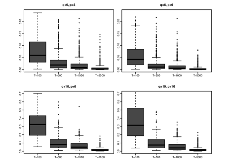
Figure 1: Example 2 – boxplots of $D_{1}(\widehat{A}_{*},{A}_{*})$ in a simulation with 1000 replications.

Example 3.

In this example we examine the gain in post-sample forecasting due to the decorrelation transformation. Now in model (1) all the elements of ${A}$ and ${B}$ are drawn independently from $U(-1,\,1)$, with $(p,q)$ equal to $(6,6)$, $(6,8)$, $(8,8)$ and $(10,10)$. For each $(p,q)$ combination, the first three rows (or columns) form one block, the next two rows (or columns) form a second block, and all the other row (or column) is independent of the rest of the rows (or columns). Table 3 shows the configuration of ${U}_{t}$ for $(p,q)=(8,8)$.

	1	2	3	4	5	6	7	8
1	.81			.64
2
3
4	.25			.25
5
6
7
8

Table 3: Example 3: Block configuration of ${U}_{t}$ for the case of $(p,q)=(8,8)$

Each univariate block of ${U}_{t}$ (e.g. $U_{t,6,6}$) is an AR(1) process with the autoregressive coefficient drawn from the $U[0.1,0.3]$ and independent and $N(0,1)$ innovations. For each block of size $(3,1)$, $(1,3)$, $(2,1)$ and $(1,2)$, a vector AR(1) model is used. All elements of the coefficient matrix is drawn independently from $U[0,1]$, then normalized so its singular values are within $[0.1,0.3]$. The vector innovations consist of independent and N$(0,1)$ random variables. Each of the remaining four blocks follow a matrix AR(1) (i.e. MAR(1)) model of Chen et al., (2021), i.e.

$${U}_{t,i,j}=\lambda_{i,j}{\Phi}_{1,i,j}{U}_{t-1,i,j}{\Phi}_{2,i,j}^{\top}+{E}_{t,i,j},\quad i,j=1,2,$$ (23)

where ${\Phi}_{1,i,j}$ and ${\Phi}_{2,i,j}$ are the coefficient matrices with unit spectral norm, all elements of ${E}_{t,i,j}$ are independent and $N(0,1)$. Matrices ${\Phi}_{1,i,j}$ and ${\Phi}_{2,i,j}$ are constructed such that their singular values are all one and the left and right singular matrices are orthonormal, and the scalar coefficient $\lambda_{i,j}$ controls the level of auto-correlation and its values for the four blocks are marked in Table 3.

We set sample sizes $T=500,1000,2000,5000$, and $(p,q)=(6,6),(8,6),(8,8),(10,10)$. For each setting, we simulate a matrix time series of length $T+M$ with $M=10$. To perform one-step ahead post-sample forecasting, for each $i=0,1,\cdots,M-1$, we use the first $T$ observations for identifying the uncorrelated blocks and for computing $\widehat{A}_{*},\widehat{B}_{*}$ and $\widehat{U}_{t}^{*}$ defined in (8). Depending on its shape/size, we fit each identified block in $\widehat{U}_{t}^{*}$ with an MAR(1), VAR(1) or AR(1) model. The fitted models are used to predict ${U}_{T+i+1}^{*}$. The predicted value for $X_{T+i+1}$ is then obtained by

$$\widehat{X}_{T+i+1}=\big{(}\widehat{\Sigma}^{(x)}_{2}\big{)}^{1/2}\widehat{B}_{*}\widehat{U}_{T+i+1}^{*}\widehat{A}_{*}^{\top}\big{(}\widehat{\Sigma}^{(x)}_{1}\big{)}^{1/2},\quad i=0,1,\cdots,M-1.$$ (24)

We then compute the mean squared error:

$${\rm MSE}=\frac{1}{pq}\sum_{i=1}^{p}\sum_{j=1}^{q}(\widehat{X}_{s,i,j}-\mu_{s,i,j})^{2},$$ (25)

where $\widehat{X}_{s,i,j}$ denote the one-step ahead predicted value for the $(i,j)$-th element $X_{s,i,j}$ of $X_{s}$, and $\mu_{s,i,j}=\mathbb{E}(X_{s,i,j}|X_{s-1},X_{s-2},\cdots)$. We compare $\widehat{X}_{s,i,j}$ with $\mu_{s,i,j}$, instead of $X_{s,i,j}$, to remove the impact of the noise in the observed $X_{s,i,j}$. We report overall the mean and the standard deviation of MSE over 1000 replications.

For the comparison purpose, we also include several other models in our simulation: (i) VAR(1) model, i.e. $X_{t}$ is stacked into a vector of length $pq$ and a VAR(1) is fitted to the vector series directly, (ii) MAR(1) model, i.e. MAR(1) of Chen et al., (2021), is fitted directly to $X_{t}$, and (iii) TS-PCA, i.e. all the elements of $X_{t}$ are stacked into a long vector and the segmentation method of Chang et al., (2018) is applied to the vector series. In addition, we also include two oracle models: (O1) the true segmentation blocks are used to model $\widehat{U}_{t}^{*}$; and (O2) True $\Sigma^{(x)}_{1},\Sigma^{(x)}_{2}$ and true ${A}_{*},{B}_{*}$ are used and the true segmentation blocks are used to model $\widehat{U}_{t}^{*}$.

The mean and standard deviations (in bracket) of the MSEs are listed in Table 4. It is clear that the forecasting based on the proposed decorrelation transformation is more accurate than those based on MAR(1), VAR(1) and TS-PCA directly. The improvement is often substantial. The only exception is the case of $(p,q)=(6,6)$ and $T=5000$: the 36-dimension VAR(1) performs marginally better (i.e. the decrease of 0.002 in MSE) than the transformation based method. On the other hand, the improvement of the transformation based forecast over VAR(1) for sample size $T\leq 2000$ is more significant. The relative poor performance of MAR(1) is due to the substantial discrepancy between MAR(1) model and the data generating mechanism used in this example. Note that there are $(p+q)^{2}$ free parameters in VAR(1) while there are merely $(p^{2}+q^{2})$ parameters in MAR(1). With large $T$, VAR(1) is more flexible than MAR(1). TS-PCA performs poorly, due to the large error in estimating the large transformation matrix of size $pq\times pq$. See also Remark 6. In addition, TS-PCA also requires to fit VAR models for several large blocks of size 9, 6, 6 and etc.

Table 4 indicates that the oracle model O1 performs only slightly better than segmentation when sample size $T=500$ or 1000. Oracle Model O2 only deviates from the true model in terms of the estimation error of the coefficients in the AR models, hence performs the best. The MSE of O2 is very close to 0, since the only source of error in MSE is the estimation error of the AR models for each blocks of $U_{t}$, which goes to zero quickly as $T$ increases since these models are of small dimensions. When $T$ is large, the VAR(1), proposed segmentation and O1 all perform about the same, which is worse than O2.

Table 4: Example 3 – One-step ahead post-sample forecasting: means and standard deviations (in bracket) of MSEs in a simulation with 1000 replications.

		MSEs and standard deviations
		$T=500$		$T=1000$		$T=2000$		$T=5000$
$(p,q)$= $(6,6)$	MAR(1)	0.515(0.333)		0.501(0.304)		0.513(0.305)		0.482(0.280)
	VAR(1)	0.369(0.142)		0.231(0.065)		0.137(0.037)		0.044(0.014)
	TS-PCA	0.492(0.232)		0.278(0.094)		0.149(0.043)		0.048(0.018)
	segmentation	0.257(0.180)		0.144(0.098)		0.087(0.094)		0.046(0.051)
	model O1	0.207(0.173)		0.098(0.079)		0.046(0.033)		0.018(0.012)
	model O2	0.018(0.010)		0.009(0.005)		0.004(0.003)		0.002(0.001)
$(p,q)$= $(6,8)$	MAR(1)	0.981(0.496)		0.977(0.491)		0.947(0.488)		0.942(0.485)
	VAR(1)	0.549(0.235)		0.323(0.111)		0.179(0.058)		0.095(0.022)
	TS-PCA	0.787(0.359)		0.442(0.168)		0.197(0.068)		0.096(0.023)
	segmentation	0.329(0.262)		0.166(0.125)		0.097(0.073)		0.061(0.049)
	model O1	0.233(0.120)		0.127(0.064)		0.078(0.041)		0.051(0.035)
	model O2	0.032(0.015)		0.016(0.007)		0.008(0.004)		0.003(0.001)
$(p,q)$= $(8,8)$	MAR(1)	0.971(0.434)		0.924(0.363)		0.915(0.391)		0.908(0.384)
	VAR(1)	0.861(0.304)		0.447(0.148)		0.275(0.079)		0.121(0.033)
	TS-PCA	0.965(0.420)		0.564(0.215)		0.290(0.106)		0.129(0.036)
	segmentation	0.499(0.276)		0.271(0.158)		0.176(0.131)		0.091(0.092)
	model O1	0.399(0.189)		0.252(0.154)		0.193(0.137)		0.120(0.133)
	model O2	0.040(0.015)		0.019(0.007)		0.010(0.004)		0.004(0.001)
$(p,q)$= $(10,10)$	MAR(1)	1.244(0.512)		1.214(0.521)		1.207(0.481)		1.218(0.509)
	VAR(1)	1.920(0.654)		1.151(0.353)		0.646(0.191)		0.354(0.078)
	TS-PCA	1.822(0.711)		1.216(0.413)		0.726(0.211)		0.365(0.128)
	segmentation	0.967(0.505)		0.664(0.326)		0.465(0.240)		0.312(0.224)
	model O1	0.852(0.403)		0.617(0.307)		0.446(0.235)		0.341(0.233)
	model O2	0.062(0.022)		0.030(0.010)		0.016(0.005)		0.006(0.002)

Example 4.

Next, we assess the sensitivity of the proposed matrix segmentation method with respective to the Kronecker product structure ($\hbox{\rm vec}(X_{t})=(A\otimes B)\hbox{\rm vec}(U_{t})$). We use the same model setting in Example 3 and choose $(p,q)=(8,8),T=500$. Instead of model (1), we consider $\hbox{\rm vec}(X_{t})=(A\otimes B+\Psi)\hbox{\rm vec}(U_{t})$, where $\Psi$ is a perturbation matrix with $N$ none-zero elements. We also set each non-zero element of $\Psi$ to be $c\|A\otimes B\|_{F}/(pq)\times\omega$, $\omega\overset{\rm iid}{\sim}$ Rademacher distribution. Table 5 shows MSEs and standard deviations of VAR(1) and the proposed matrix segmentation method over 1000 replications, for several combinations of $N$ and $c$. Again, $N$ controls the number of non-zero perturbations and $c$ controls the level of the perturbations, comparing to the average size of the elements in $A\otimes B$. When $c=0$, it becomes the original case in Table 4. From Table 5, it is seen that the segmentation is still useful in prediction when the model is deviated from the assumed block structure within certain perturbation. The prediction performance of the VAR model is not affected by the perturbation since it does not assume any block structure. It is seen that the segmentation outperforms the VAR model when $c<0.3$ when $N=10$ and $c<0.2$ when $N=100$. This feature demonstrates the benefit of dimension reduction through segmentation, even when the underlying model does not have the exact Kronecker product structure.

Table 5: Sensitivity of the Kronecker product structure using different $N$ and $c$. The results are the means and standard deviations (in bracket) of MSEs of one-step ahead post-sample forecasting based on 1000 replications.

		MSEs and standard deviations
		$c=0$	$c=0.05$	$c=0.15$	$c=0.2$	$c=0.3$
$N=10$	VAR(1)	0.861(0.304)	0.877(0.327)	0.872(0.314)	0.874(0.291)	0.869(0.306)
	segmentation	0.499(0.276)	0.490(0.241)	0.620(0.303)	0.732(0.399)	0.859(0.504)
$N=100$	VAR(1)	0.861(0.304)	0.856(0.295)	0.860(0.303)	0.874(0.326)	0.878(0.317)
	segmentation	0.499(0.276)	0.570(0.314)	0.721(0.458)	0.856(0.530)	0.976(0.689)

4.2 Real data analysis

We now illustrate the proposed decorrelation method with a real data example. The data concerned is a 17$\times$6 matrix time series consisting of the logarithmic daily averages of the 6 air pollutant concentration readings (i.e. PM_2.5, PM₁₀, SO₂, NO₂, CO, O₃) from the 17 monitoring stations in Beijing and its surrounding areas (i.e. Tianjin and Hebei Province) in China. The sampling period is January 1, 2015 – December 31, 2016 for a total of $T=731$ days. The readings of different pollutants at different locations are crossly correlated.

We first remove the seasonal mean of the $17\times 6$ matrix time series. Setting $\tau_{0}=5$ in (7), we apply the proposed bilinear transformation to discover the uncorrelated block structure. The finding is stable: with $5\leq\tau_{1}\leq 30$ in (10), the transformed matrix series admits $\widehat{n}_{c}=4$ uncorrelated column blocks with sizes $3,1,1,1$ respectively, and $\widehat{n}_{r}=15$ uncorrelated row blocks with two blocks of size 2 and the rest of size 1. Overall there are $15\times 4$ blocks, among which there are 2 blocks of size $2\times 3$, 13 blocks of size $1\times 3$, 6 blocks of size $2\times 1$ and 39 blocks of size $1\times 1$.

To check the post-sample forecasting performance, we calculate the rolling one-step, and two-step ahead out-sample forecasts for each of the daily readings in the last three months in 2016 (total 92 days). The methods included in the comparison are (i) the forecasting based on the segmentation derived from the proposed decorrelation transformation by fitting an MAR(1), VAR(1) or AR(1) to each identified block according to its size and shape; (ii) MAR(1) for the original $17\times 6$ matrix series; (iii) VAR(1) for the vectorized original series, (iv) univariate AR(1) for each of the $17\times 6$ original series, and (v) the TS-PCA (Chang et al.,, 2018) for the vectorized original series. The TS-PCA leads to the segmentation consisting of one group of size 3, three groups of size 2, and 93 groups of size 1. For each group, a VAR(1) model is used for prediction.

For the two segmentation approaches, we fix the needed transformation obtained using data up to September 30, 2016, and the corresponding segmentation structure. The time series model for each individual block is updated throughout the rolling forecasting period.

In addition to the identified segmentation with 15$\times$4 blocks, we also compute the forecasts based on two other segmentations: one with 14$\times$3 blocks, and another with 16$\times$5 blocks. The former is obtained by merging two most correlated single row blocks in the discovered segmentation into one block and two most correlated single column blocks into one block. The latter is obtained by splitting one of the two blocks with two rows in the discovered segmentation into two single row blocks and splitting the block with 3 columns into two blocks. This will reveal the impact of slightly ‘wrong’ segmentations on forecasting performance.

Table 6: One-step and two-step ahead post-sample forecasting for the air pollution data: means and standard deviations (in bracket) of MSPE_s, regrets and adjusted ratios of the various methods.

Method	One-step forecast			Two-step forecast
	raw forecast	regret	adjust ratio	raw forecast	regret	adjust ratio
MAR(1)	0.351 (0.208)	0.154	1.305	0.516 (0.303)	0.319	1.340
VAR(1)	0.400 (0.272)	0.203	1.720	0.717 (0.406)	0.520	2.185
Univariate AR	0.346 (0.205)	0.149	1.263	0.501 (0.286)	0.304	1.277
TS-PCA	0.332 (0.188)	0.135	1.144	0.450 (0.247)	0.253	1.063
Segmentation with 15$\times$4 blocks	0.315 (0.182)	0.118	1.000	0.435 (0.246)	0.238	1.000
Segmentation with 14$\times$3 blocks	0.319 (0.185)	0.122	1.034	0.446 (0.256)	0.249	1.046
Segmentation with 16$\times$5 blocks	0.318 (0.183)	0.121	1.025	0.443 (0.247)	0.246	1.034

Let the mean squared forecast error for $s$-th observation be

$${\rm MSPE}_{s}=\frac{1}{pq}\sum_{i=1}^{p}\sum_{j=1}^{q}(\widehat{X}_{s,i,j}-X_{s,i,j})^{2},$$ (26)

where $\widehat{X}_{s,i,j}$ denote the one-step ahead predicted value for the $(i,j)$-th element $X_{s,i,j}$ of $X_{s}$. Two-step ahead MSPE_s is defined similarly. The means and the standard deviations of MSPE_s of one-step and two-step ahead post-sample forecasts for the pollution readings in the last 92 days are listed in Table 6. The prediction based on the bilinear decorrelation transformation (even using ‘wrong’ segmentations) is clearly more accurate than those without transformation as well as that of the TS-PCA. Using the ‘wrong’ segmentation deteriorates the performance only slightly, indicating that a partial (instead of total) decorrelation still leads to significant gain in prediction. Applying TS-PCA to the vectorized series requires to estimate a $102\times 102$ transformation matrix (instead of the $17\times 17$ and $6\times 6$ matrices by utilizing the matrix time series structure). It leads to larger estimation errors (see Remark 6 in Section 3). Nevertheless it still provides more accurate predicts than those without transformation. Also note that fitting each of the original $17\times 6$ time series with a univariate AR(1) separately leads to a better performance than those from fitting MAR(1) and VAR(1) to the original matrix series jointly. This indicates that the cross-serial correlation is useful and important information for future forecasting. However to make efficient use of the information, it is necessary to adopt some effective independent component analysis or dimension-reduction techniques such as the proposed decorrelation transformation which pushes correlations across different series into the autocorrelations of some transformed series.

Also included in the table are ‘regret’ defined as the difference between MSPE and the in-sample residual variance of the fitted VAR(1) model for the vectorized data (i.e. a vector time series of dimension $17\times 6=102$), and ‘adjusted ratio’ defined as the ratio of the regret to the regret of the best prediction model (i.e. the segmentation with $15\times 4$ blocks). The regret tries to measure the forecasting error on the predictable signal, removing the impact from unpredictable noise in the model. Since the fitted VAR(1) model uses more than 10,000 parameters, its sample residual variance underestimates the noise variance in the model, and is taken as a proxy for the latter. The adjusted ratios shows that the ‘regret’ of TS-PCA is 14.4% worse than the $15\times 4$ segmentation for one-step ahead forecast, and 6.4% worse than the $15\times 4$ segmentation for two-step ahead forecast.

To further evaluate the forecasting stability, Figure 2 shows weekly average of one-step rolling forecast MSPE within the forecasting period under various models. It is seen that the proposed segmentation outperforms the other three methods in most of the periods in terms of prediction.

Figure 2: Weakly averaged one-step forecast errors of the univariate AR(1) models for each component series (AR), the matrix AR(1) model (MAR(1)), the vector AR(1) for vectorized series (VAR(1)), the method based on the bilinear decorrelation transformation (segmentation).

In this example, the identified segmentation of $(\widehat{n}_{r},\widehat{n}_{c})=(15,4)$ for the original 17$\times$6 matrix series is more likely to be an approximation of the underlying dependence structure rather than a true model. The fact that the two ‘wrong’ segmentation models (though quite close to the discovered one) as well as the aggressive segmentation via vectorized TS-PCA transformation provide comparable, though inferior, post-sample forecasting performance lends further support to the claim that the proposed decorrelation method makes the transformed series more predictable than the original ones, regardless model (1) holds or not. See Remark 1(iv) in Section 2.1 above.

Appendix A Additional simulation results

Example 5.

In this example we provide some sensitivity analysis with the tuning parameters $\tau_{0}$ in (4) and $\tau_{1}$ in (10), as discussed in Remark 5(ii). Again, we use the same model setting in Example 3 and choose $(p,q)=(8,8),T=500$. Note that $\tau_{0}=5$ and $\tau_{1}=15$ are used in Example 3. Figure 3 shows the average of post sample MSEs over 1000 independent Monte Carlo experiments for different combinations of $\tau_{0}$ and $\tau_{1}$. It can be seen from Figure 3(a) that except $\tau_{0}=1$, the segmentation performance remains relatively stable for different values of $\tau_{0}$. Similarly, Figure 3(b) shows that the segmentation performance using different $\tau_{1}$ is also relatively stable. Since the data generating process is an AR process of order 1, the cross-autocorrelations are the largest at the small lags, hence only a relatively small $\tau_{1}$ is needed in this case. Overall, the MSE does not change much with $\tau_{0},\tau_{1}$.

(a) Effect of $\tau_{0}$ (fix $\tau_{1}=15$)

(b) Effect of $\tau_{1}$ (fix $\tau_{0}=5$)

Figure 3: Sensitivity analysis with changing $\tau_{0}$ and $\tau_{1}$

Appendix B Additional information on the air pollutant example

In this appendix we provide additional figures of the air pollutant data used in the real data analysis. Figure 4 displays the time series plot of the $17\times 6=102$ series after removing the seasonal means. Figure 5 shows the cross correlogram of five randomly selected stations for PM₁₀, and Figure 6 displays the cross correlogram of all six pollutants for a station in Beijing.

Figure 4: Time series plot of 17 by 6 air pollution data

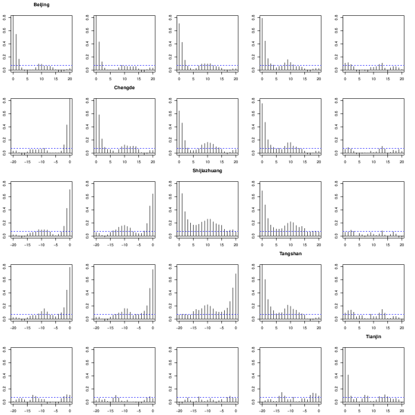
Figure 5: Cross correlogram of logarithmic daily PM₁₀ readings at five randomly selected monitoring stations in Beijing, Tianjin and Hebei

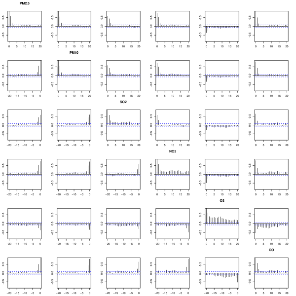
Figure 6: Cross correlogram of logarithmic daily readings of all six pollutants for a station in Beijing

Appendix C Proofs

Proof of Proposition 2.

In the following we provide the construction of ${A}_{*}={\Gamma}^{(1)}{}$, where the columns of ${\Gamma}^{(1)}$ is the $q$ orthonormal eigenvectors of ${W}^{(1)}$ and is a column permutation matrix. Let

$$Z_{t}^{*}={B}{U}_{t};\quad{\Sigma}_{1}^{(u)}=\mathbb{E}(Z_{t}^{*\top}Z_{t}^{*});\quad Z_{t}=Z_{t}^{*}\big{(}{\Sigma}_{1}^{(u)}\big{)}^{-1/2}$$

Clearly, ${\Sigma}_{1}^{(u)}$ is block diagonal. Hence, the column of $Z_{t}$ has same uncorrelated (segmentation) structure as that of $Z_{t}^{*}$.

We have

$$\overrightarrow{X_{t}}:={B}{U}_{t}{A}^{\top}({\Sigma}_{1}^{(x)})^{-1/2}=Z_{t}^{*}{A}^{\top}({\Sigma}_{1}^{(x)})^{-1/2}=Z_{t}A_{*}^{\top}$$ (27)

where $A_{*}=\big{(}{\Sigma}_{1}^{(x)}\big{)}^{-1/2}{A}\big{(}{\Sigma}_{1}^{(u)}\big{)}^{1/2}$. Note that $\mathbb{E}(Z_{t}^{\top}Z_{t})/p={I}_{q}=\mathbb{E}(\overrightarrow{X_{t}}^{\top}\overrightarrow{X_{t}})/p$, where ${I}_{q}$ is the $q\times q$ identity matrix. Hence $A_{*}$ is orthonormal. Note that $B_{*}$ can be similarly defined.

Let the auto-cross-covariance matrices between the $i$-th and the $j$-th rows of $\overrightarrow{X_{t}}$ and the corresponding $Z_{t}$ at lag $\tau$ be

$${V}^{(1)}_{\tau,i,j}=\mathbb{E}\{\overrightarrow{X}_{t+\tau}^{\top}{E}_{i,j}\overrightarrow{X_{t}}\},\mbox{\ \ and \ \ }{V}^{(z)}_{\tau,i,j}=\mathbb{E}\{{Z}_{t+\tau}^{\top}{E}_{i,j}Z_{t}\},$$

where ${E}_{i,j}={\mathbf{e}}_{i}{\mathbf{e}}_{j}^{\top}\in{{\mathbb{R}}}^{p\times p}$ is the unit matrix with 1 at position $(i,j)$ and 0 elsewhere. Let

$${W}^{(1)}=\sum_{\tau=-\tau_{0}}^{\tau_{0}}\sum_{i=1}^{p}\sum_{j=1}^{p}\frac{{V}^{(1)}_{\tau,i,j}\big{(}{V}^{(1)}_{\tau,i,j}\big{)}^{\top}}{p^{2}},\mbox{\ \ and \ \ }{W}^{(z)}=\sum_{\tau=-\tau_{0}}^{\tau_{0}}\sum_{i=1}^{p}\sum_{j=1}^{p}\frac{{V}^{(z)}_{\tau,i,j}\big{(}{V}^{(z)}_{\tau,i,j}\big{)}^{\top}}{p^{2}}.$$ (28)

Since $Z_{t}$ has a column-wise uncorrelated structure, ${V}^{(z)}_{\tau,i,j}$ is block diagonal for all $i,j$. Hence, ${W}^{(z)}$ is block diagonal as well. Let

$${W}^{(z)}=\begin{pmatrix}{W}^{(z)}_{1}&0&\cdots&0\cr 0&{W}^{(z)}_{2}&\cdots&0\cr\vdots&\vdots&\ddots&\vdots\cr 0&0&\cdots&{W}^{(z)}_{n_{c}}\end{pmatrix}.$$ (29)

Write the eigenvalue decomposition of each ${W}_{i}^{(z)}$ in (29) as

$${W}_{i}^{(z)}={\Gamma}_{i}^{(z)}{D}_{i}\big{(}{\Gamma}_{i}^{(z)}\big{)}^{\top},$$ (30)

where ${\Gamma}_{i}^{(z)}$ is a $q_{i}\times q_{i}$ orthogonal matrix and ${D}_{i}$ is a diagonal matrix, consists of the eigenvalues of ${W}^{(z)}_{i}$ in descending order $\lambda_{i1}\geq\lambda_{i2}\geq\ldots\geq\lambda_{iq_{i}}$. Hence we can write

$${W}^{(z)}={\Gamma}^{(z)}{D}\big{(}{\Gamma}^{(z)}\big{)}^{\top},$$ (31)

where

$${\Gamma}^{(z)}=\hbox{\rm diag}\big{(}{\Gamma}^{(z)}_{1},\cdots,{\Gamma}^{(z)}_{n_{c}}\big{)},\quad\quad{D}=\hbox{\rm diag}\big{(}{D}_{1},\cdots,{D}_{n_{c}}\big{)},$$ (32)

with ${\Gamma}^{(z)}$ orthogonal. Let the eigenvalue decomposition of ${W}^{(z)}$ (as a whole) be

$${W}^{(z)}={\Gamma}^{(z*)}{D}^{*}\big{(}{\Gamma}^{(z*)}\big{)}^{\top},$$ (33)

where the eigenvalues in the diagonal matrix ${D}^{*}$ is in descending order. Comparing (31) and (33), these exists a column permutation matrix such that ${\Gamma}^{(z*)}={\Gamma}^{(z)}{}^{\top}$, and ${D}^{*}={}{D}{}^{\top}$.

Since $\overrightarrow{X_{t}}=Z_{t}A_{*}^{\top}$ in (27), we have ${V}^{(1)}_{\tau,i,j}=A_{*}{V}^{(z)}_{\tau,i,j}A_{*}^{\top}$, Hence

$${W}^{(1)}=A_{*}{W}^{(z)}A_{*}^{\top}=A_{*}{\Gamma}^{(z)}{D}({\Gamma}^{(z)})^{\top}A_{*}^{\top}=A_{*}{\Gamma}^{(z*)}{D}^{*}A_{*}({\Gamma}^{(z*)})^{\top}A_{*}^{\top}={\Gamma}^{(1)}{D}^{*}\big{(}{\Gamma}^{(1)}\big{)}^{\top}$$

where ${\Gamma}^{(1)}=A_{*}{\Gamma}^{(z*)}$. Since ${\Gamma}^{(1)}$ is an orthogonal matrix and ${D}^{*}$ is a diagonal matrix with descending diagonals, it is clear that ${D}^{*}$ contains the eigenvalues of ${W}^{(1)}$ and ${\Gamma}^{(1)}$ contains the corresponding eigenvectors.

Now it follows from (27) that

$$\overrightarrow{X_{t}}{\Gamma}^{(1)}=Z_{t}A_{*}^{\top}A_{*}{\Gamma}^{(z*)}=Z_{t}{\Gamma}^{(z*)}=Z_{t}{\Gamma}^{(z)}{}^{\top}.$$ (34)

Or

$$\overrightarrow{X_{t}}{\Gamma}^{(1)}{}=Z_{t}{\Gamma}^{(z)}.$$ (35)

Since the columns of $Z_{t}{\Gamma}^{(z)}=\overrightarrow{X_{t}}{\Gamma}^{(1)}{}$ has the same uncorrelated structure as that of $Z_{t}$, ${\Gamma}^{(1)}{}$ is the desired orthogonal transformation ${A}_{*}$ we are looking for. ∎

As $|{\mathbb{P}}({\cal E}_{1}\cap{\cal E}_{2})-{\mathbb{P}}({\cal E}_{1}){\mathbb{P}}({\cal E}_{2})|\leq 1/4\leq e^{-1}$ for all event pairs $\{{\cal E}_{1},{\cal E}_{2}\}$,

$$\sup_{t}\Big{\{}\Big{|}{\mathbb{P}}({\cal E}_{1}\cap{\cal E}_{2})-{\mathbb{P}}({\cal E}_{1}){\mathbb{P}}({\cal E}_{2})\Big{|}:{\cal E}_{1}\in\sigma(X_{s+\tau}\otimes X_{s},s\leq t,\tau\leq\tau_{0}),{\cal E}_{2}\in\sigma(X_{s+\tau}\otimes X_{s},s\geq t+k)\Big{\}}$$

$$\leq \sup_{t}\Big{\{}\Big{|}{\mathbb{P}}({\cal E}_{1}\cap{\cal E}_{2})-{\mathbb{P}}({\cal E}_{1}){\mathbb{P}}({\cal E}_{2})\Big{|}:{\cal E}_{1}\in\sigma(X_{s},s\leq t+\tau_{0}),{\cal E}_{2}\in\sigma(X_{s},s\geq t+k)\Big{\}}$$

$$\leq \exp\Big{[}-\max\{1,c_{0}(k-\tau_{0})^{r_{1}}\}\Big{]}$$

$$\leq \exp\Big{[}-c_{0}(1+c_{0}^{1/r_{1}}\tau_{0})^{-r_{1}}k^{r_{1}}\Big{]},$$

where $\otimes$ denotes the Kronecker product for matrices. Thus, the quadratic process $(X_{t+\tau}\otimes X_{t},0\leq\tau\leq\tau_{0})$ also satisfies the $\alpha$-mixing condition with $c_{0}$ in Assumption 1 replaced by the smaller $c_{0}(1+c_{0}^{1/r_{1}}\tau_{0})^{-r_{1}}$.

Proof of Theorem 1..

As $\|{V}\|_{\rm op}\leq q\|{V}\|_{\max}$ for all matrices ${V}\in{{\mathbb{R}}}^{q\times q}$, it suffices to bound the estimation error under the $\|\cdot\|_{\max}$ norm. In the proof, we consider a more general case that $\mathbb{E}X_{t}$ is not necessary 0 and let

$$\widehat{\Sigma}^{(1)}_{\tau,i,j}=\sum_{t=1}^{T-\tau}{({X}_{t+\tau}-\widehat{\mu}_{\tau,+})^{\top}{E}_{i,j}(X_{t}-\widehat{\mu}_{\tau,-})\over T-\tau},\;\;\widehat{\Sigma}_{1}^{(x)}=\frac{1}{p}\sum_{i=1}^{p}\widehat{\Sigma}^{(1)}_{0,i,i},$$

and

$$\widehat{\mu}_{\tau,+}=\frac{\sum_{t=1}^{T-\tau}X_{t+\tau}}{T-\tau},\;\;\widehat{\mu}_{\tau,-}=\frac{\sum_{t=1}^{T-\tau}X_{t}}{T-\tau},\;\;{\widetilde{\Sigma}}^{(1)}_{\tau,i,j}=\sum_{t=1}^{T-\tau}\frac{X_{t+\tau}{E}_{i,j}X_{t}}{T-\tau}.$$

Note that $\widetilde{e}_{k}^{\top}({\widetilde{\Sigma}}^{(1)}_{\tau,i,j}-{\Sigma}^{(1)}_{\tau,i,j})\widetilde{e}_{l}=X_{t+\tau,i,k}X_{t,j,l}-\mathbb{E}X_{t+\tau,i,k}X_{t,j,l}$, where $\widetilde{e}_{k}$ is a $q\times 1$ vector with 1 at $k$th element and 0 otherwise. Pick $a>0$ and $u>\mathbb{E}X_{t+\tau,i,k}X_{t,j,l}$, then

$${\mathbb{P}}\left(|X_{t+\tau,i,k}X_{t,j,l}-\mathbb{E}X_{t+\tau,i,k}X_{t,j,l}|>u\right)$$

$$= {\mathbb{P}}\left(|X_{t+\tau,i,k}X_{t,j,l}-\mathbb{E}X_{t+\tau,i,k}X_{t,j,l}|>u,|X_{t+\tau,i,k}|>u^{a}\right)$$

$$\quad+{\mathbb{P}}\left(|X_{t+\tau,i,k}X_{t,j,l}-\mathbb{E}X_{t+\tau,i,k}X_{t,j,l}|>u,|X_{t+\tau,i,k}|\leq u^{a}\right)$$

$$\leq {\mathbb{P}}\left(|X_{t+\tau,i,k}|>u^{a}\right)+{\mathbb{P}}\left(|X_{t,j,l}|>u^{1-a}\right)$$

$$\leq c_{1}\exp(-c_{2}u^{ar_{2}})+c_{1}\exp(-c_{2}u^{(1-a)r_{2}})$$

$$\leq 2c_{1}\exp(-c_{2}u^{r_{2}/2}).$$

Let $1/\beta_{1}=1/r_{1}+2/r_{2}$ and $1/\beta_{2}=1/r_{1}+1/r_{2}$. Hence, by Theorem 1 of Merlevède et al., (2011), Bernstein inequality for $\alpha$ strong mixing processes, we have

$${\mathbb{P}}\left(|\widetilde{e}_{k}^{\top}({\widetilde{\Sigma}}^{(1)}_{\tau,i,j}-{\Sigma}^{(1)}_{\tau,i,j})\widetilde{e}_{l}|\geq x\right) \leq T\exp\left(-C_{1}T^{\beta_{1}}x^{\beta_{1}}\right)+\exp\left(-C_{2}Tx^{2}\right),$$

$${\mathbb{P}}\left(|\widetilde{e}_{k}^{\top}\widehat{\mu}_{\tau,+}^{\top}E_{ij}\widehat{\mu}_{\tau,-}\widetilde{e}_{l}|\geq x\right) \leq T\exp\left(-C_{1}T^{\beta_{2}}x^{\beta_{2}/2}\right)+\exp\left(-C_{2}Tx\right).$$

Then,

$${\mathbb{P}}\left(|\widetilde{e}_{k}^{\top}(\widehat{\Sigma}^{(1)}_{\tau,i,j}-{\Sigma}^{(1)}_{\tau,i,j})\widetilde{e}_{l}|\geq x\right)\leq T\exp\left(-CT^{\beta_{1}}x^{\beta_{1}}\right)+T\exp\left(-CT^{\beta_{2}}x^{\beta_{2}/2}\right)$$

$$+\exp\left(-CTx^{2}\right)+\exp\left(-CTx\right).$$

With probability at least $1-\epsilon_{T}$, for any $1\leq i,j\leq p$, we have

$$\left\|\widehat{\Sigma}^{(1)}_{\tau,i,j}-{\Sigma}^{(1)}_{\tau,i,j}\right\|_{\max}\leq C_{1}^{\prime}\sqrt{\frac{\log(pq/\epsilon_{T})}{T}}+C_{1}^{\prime}\frac{[\log(Tpq/\epsilon_{T})]^{1/\beta_{1}}}{T}+C_{1}^{\prime}\frac{[\log(Tpq/\epsilon_{T})]^{2/\beta_{2}}}{T^{2}}.$$ (36)

Then (15) follows. The proof is complete as (16) follows from Wedin’s theorem, (15), (6), and (7). By Wedin’s theorem, (16) implied directly that $||\hat{\Gamma}^{(1)}-\Gamma^{(1)}||\leq C_{2}\eta_{T,p,q}$. Hence (18) holds by Proposition 2 and Lemma 1. ∎

Proof of Theorem 2..

From Assumption 5, it yields

$$\max_{t}\max_{i,j,k,l}{\mathbb{P}}\left(|X_{t_{\tau},i,k}X_{t,j,l}-\mathbb{E}X_{t_{\tau},i,k}X_{t,j,l}|>u\right)\leq c_{1}^{\prime}x^{-r_{1}}.$$

By the Fuk-Nagaev type inequality stated in Theorem 6.2, or equation (6.19a), of Rio, (2000),

$${\mathbb{P}}\left(|\widetilde{e}_{k}^{\top}({\widetilde{\Sigma}}^{(1)}_{\tau,i,j}-{\Sigma}^{(1)}_{\tau,i,j})\widetilde{e}_{l}|\geq x\right) \leq 4\exp(-C_{1}Tx^{2})+4C_{2}T(Tx)^{-\frac{(r_{1}+1)r_{2}}{r_{1}+r_{2}}},$$

$${\mathbb{P}}\left(|\widetilde{e}_{k}^{\top}\widehat{\mu}_{\tau,+}^{\top}E_{ij}\widehat{\mu}_{\tau,-}\widetilde{e}_{l}|\geq x\right) \leq 4\exp(-C_{1}Tx^{2})+4C_{2}T(Tx)^{-\frac{2(r_{1}+1)r_{2}}{r_{1}+2r_{2}}}.$$

Then,

$${\mathbb{P}}\left(|\widetilde{e}_{k}^{\top}(\widehat{\Sigma}^{(1)}_{\tau,i,j}-{\Sigma}^{(1)}_{\tau,i,j})\widetilde{e}_{l}|\geq x\right)\leq CT(Tx)^{-\frac{(r_{1}+1)r_{2}}{r_{1}+r_{2}}}+8\exp(-C_{1}Tx^{2}).$$

Let $\beta_{3}=r_{2}(r_{1}+1)/(r_{1}+r_{2})>1$. With probability at least $1-\epsilon_{T}$, for any $1\leq i,j\leq p$, we have

$$\left\|\widehat{\Sigma}^{(1)}_{\tau,i,j}-{\Sigma}^{(1)}_{\tau,i,j}\right\|_{\max}\leq C_{1}^{\prime}\frac{(Tpq/\epsilon_{T})^{1/\beta_{3}}}{T}+C_{1}^{\prime}\sqrt{\frac{\log(pq/\epsilon_{T})}{T}}.$$ (37)

The rest is the same as the proofs in Theorem 1. ∎

For any group $G\subset\{1,\ldots,q\}$, define the eigengap as

$$\Delta_{G}=\min\Big{\{}|\lambda_{j}-\lambda_{k}|:j\in G,k\not\in G\Big{\}}.$$ (38)

Let ${\Gamma}_{G}^{(1)}=({\gamma}_{j})_{j\in G}$. We say that the group $G$ is identifiable if $\Delta_{G}>0$ as the column space of ${\Gamma}^{(1)}_{G}$ would then be the span of $|G|$ eigenvectors for all versions of ${\Gamma}^{(1)}$.

Lemma 1.

Suppose conditions of Theorem 1 (resp. Theorem 2) hold. For a certain $G\subset\{1,\ldots,q\}$, assume $C_{1}\eta_{T,p,q}<\Delta_{G}/2$ with the $\eta_{T,p,q}$ in (17) and $C_{1}$ given in Theorem 1 (resp. Theorem 2) depending on $c_{*},c^{*},r_{1},r_{2}$ only. Let ${P}_{G}={\Gamma}^{(1)}_{G}\Big{(}{\Gamma}^{(1)}_{G}\Big{)}^{\top}$ be the orthogonal projection to the corresponding eigenspace, and $\widehat{P}_{G}=\widehat{\Gamma}^{(1)}_{G}\Big{(}\widehat{\Gamma}^{(1)}_{G}\Big{)}^{\top}$ be the sample version. Then, in the event $\Omega_{T}$ given in Theorem 1 (resp. Theorem 2) with probability at least $1-\epsilon_{T}$, by (16),

$$\Big{\|}\widehat{P}_{G}-{P}_{G}\Big{\|}_{\rm op}\leq\frac{C_{1}\eta_{T,p,q}}{\Delta_{G}-C_{1}\eta_{T,p,q}}<1.$$ (39)

By the structure assumption in (1), there exists a group structure $G_{c}=\{G_{1},...,G_{n_{c}}\}$, such that the columns of different groups

$$X_{t}\Big{(}{\Sigma}^{(1)}_{1}\Big{)}^{-1/2}{\Gamma}^{(1)}_{G_{i}},\ i=1,\ldots,n_{c},$$ (40)

are uncorrelated across all time lags. Let $G$ be one of the $G_{i}$ or a union of several $G_{i}$. It follows from Lemma 1 that when the group $G$ is identifiable with a sufficiently large eigengap $\Delta_{G}$, ${\cal M}(\widehat{A}_{*G})$ is a consistent estimator of the subspace ${\cal M}(A_{*G})$, even in the presence of tied eigenvalues within $G$ or within $G^{c}$.

Proof of Theorem 3..

Let $U\hbox{\rm diag}(\phi_{1},\ldots,\phi_{r})\widehat{U}^{\top}$ be the SVD of ${P}_{G_{i_{0}}}\widehat{P}_{G_{i_{0}}}$ with $\phi_{1}\geq\cdots\geq\phi_{r}$ and $n_{i_{0}}=|G_{i_{0}}|$, $1\leq i_{0}\leq n_{c}$. Define ${\Pi}_{G_{i_{0}}}=U\widehat{U}^{\top}\widehat{\Gamma}^{(1)}_{G_{i_{0}}}$. As $\widehat{U}\widehat{U}^{\top}=\widehat{P}_{G_{i_{0}}}=\widehat{\Gamma}^{(1)}_{G_{i_{0}}}\big{(}\widehat{\Gamma}^{(1)}_{G_{i_{0}}}\big{)}^{\top}$, ${\Pi}_{G_{i_{0}}}$ has orthonormal columns. Note that $UU^{\top}={\Gamma}^{(1)}_{G_{i_{0}}}\big{(}{\Gamma}^{(1)}_{G_{i_{0}}}\big{)}^{\top}$. Moreover,

$$\|{\Pi}_{G_{i_{0}}}-\widehat{\Gamma}^{(1)}_{G_{i_{0}}}\|_{\rm op}=\|(U-\widehat{U})\widehat{U}^{\top}\widehat{\Gamma}^{(1)}_{G_{i_{0}}}\|_{\rm op}\leq\|U-\widehat{U}\|_{\rm op}=\max_{1\leq j\leq n_{i_{0}}}\|(U-\widehat{U}){\mathbf{e}}_{j}\|_{2}.$$

Let $u_{j}=U{\mathbf{e}}_{j}$ and $\widehat{u}_{j}=\widehat{U}{\mathbf{e}}_{j}$, where $e_{j}$ is a $q\times 1$ vector with 1 at $j$-th element and 0 otherwise. As

$$({P}_{G_{i_{0}}}-\widehat{P}_{G_{i_{0}}})(u_{j},\widehat{u}_{j})=(u_{j}-\widehat{U}\widehat{U}^{\top}Ue_{j},UU^{\top}\widehat{U}e_{j}-\widehat{u}_{j})=(u_{j}-\phi_{j}\widehat{u}_{j},\phi_{j}u_{j}-\widehat{u}_{j}),$$

the span of the columns $u_{j}$ and $\widehat{u}_{j}$ forms invariance subspaces of ${P}_{G_{i_{0}}}-\widehat{P}_{G_{i_{0}}}$. Then a linear combination of $u_{j}$ and $\widehat{u}_{j}$ forms eigenvectors of ${P}_{G_{i_{0}}}-\widehat{P}_{G_{i_{0}}}$. Elementary calculation shows that ${P}_{G_{i_{0}}}-\widehat{P}_{G_{i_{0}}}$ has eigenvectors $u_{j}-\phi_{j}^{-1}\big{(}1\pm\sqrt{1-\phi_{j}^{2}}\big{)}\widehat{u}_{j}$. As

$$0=\Big{\langle}u_{j}-\phi_{j}^{-1}\big{(}1+\sqrt{1-\phi_{j}^{2}}\big{)}\widehat{u}_{j},u_{j}-\phi_{j}^{-1}\big{(}1-\sqrt{1-\phi_{j}^{2}}\big{)}\widehat{u}_{j}\Big{\rangle}=1-2u_{j}^{\top}\widehat{u}_{j}/\phi_{j}+1,$$

$\|(U-\widehat{U}){\mathbf{e}}_{j}\|_{2}^{2}=2(1-\phi_{j})$, so that by Lemma 1, if $2C_{1}\eta_{T,p,q}<\Delta$, then

$$\|{\Pi}_{G_{i_{0}}}-\widehat{\Gamma}^{(1)}_{G_{i_{0}}}\|_{\rm op}^{2}=2(1-\phi_{r})\leq 2\Big{(}1-\sqrt{1-\|{P}_{G_{i_{0}}}-\widehat{P}_{G_{i_{0}}}\|_{\rm op}^{2}}\Big{)}\leq 8C_{1}^{2}\eta_{T,p,q}^{2}/\Delta^{2}.$$

For this potentially random ${\Pi}_{G_{i_{0}}}$, the inseparability condition provides a $\rho^{*}$-connection graph $(G_{i_{0}},E_{i_{0}})$ with $H_{i_{0}}=G_{i_{0}}$. As the eigenvalues of ${V}^{(1)}_{0,j,j}$ are within $[c_{*}/c^{*},c^{*}/c_{*}]$, for $(k,\ell)\in E_{i_{0}}$ and in an event $\Omega_{T}$ with probability at least $1-\epsilon_{T}$,

$$\left|\big{\langle}\widehat{\gamma}_{k},\widehat{V}^{(1)}_{0,i,i}\widehat{\gamma}_{k}\big{\rangle}-\big{\langle}\widehat{\gamma}_{k},{V}^{(1)}_{0,i,i}\widehat{\gamma}_{k}\big{\rangle}\right|\leq C_{1}\eta_{T,p,q}\leq(C_{1}c^{*}\eta_{T,p,q}/c_{*})\big{\langle}\widehat{\gamma}_{k},{V}^{(1)}_{0,i,i}\widehat{\gamma}_{k}\big{\rangle},$$

$$\left|\big{\langle}\widehat{\gamma}_{k},{V}^{(1)}_{0,i,i}\widehat{\gamma}_{k}\big{\rangle}-\big{\langle}{\gamma}_{k},{V}^{(1)}_{0,i,i}{\gamma}_{k}\big{\rangle}\right|\leq 2(c^{*}/c_{*})\|\widehat{\gamma}_{k}-{\gamma}_{k}\|_{\rm op}\leq 4\sqrt{2}(C_{1}c^{*}/c_{*})\eta_{T,p,q}/\Delta,$$

in view of $\|\widehat{\gamma}^{(1)}_{k}-{\gamma}_{k}\|_{\rm op}\leq\|{\Pi}_{G_{i_{0}}}-\widehat{\Gamma}^{(1)}_{G_{i_{0}}}\|_{\rm op}\leq 2\sqrt{2}C_{1}\eta_{T,p,q}/\Delta$. Thus, for any $1\leq i_{0}\leq n_{c}$ and $k,\ell\in G_{i_{0}}$,

$$\widehat{\rho}^{(1)}_{k,\ell} \geq \frac{1}{1+C_{1}c^{*}\eta_{T,p,q}/c_{*}}\max_{i,j,\tau}\frac{\big{|}\big{\langle}\widehat{\gamma}_{k},\widehat{V}^{(1)}_{\tau,i,j}\widehat{\gamma}_{\ell}\big{\rangle}\big{|}}{\big{\{}\big{\langle}\widehat{\gamma}_{k},{V}^{(1)}_{0,i,i}\widehat{\gamma}_{k}\big{\rangle}\big{\langle}\widehat{\gamma}_{\ell},{V}^{(1)}_{0,j,j}\widehat{\gamma}_{\ell}\big{\rangle}\big{\}}^{1/2}}$$

$$\geq \frac{(1+4\sqrt{2}C_{1}c^{*2}\eta_{T,p,q}/(c_{*}^{2}\Delta))^{-1}}{1+C_{1}c^{*}\eta_{T,p,q}/c_{*}}\max_{i,j,\tau}\frac{\big{|}\big{\langle}\widehat{\gamma}_{k},\widehat{V}^{(1)}_{\tau,i,j}\widehat{\gamma}_{\ell}\big{\rangle}\big{|}}{\big{\{}\big{\langle}{\gamma}_{k},{V}^{(1)}_{0,i,i}{\gamma}_{k}\big{\rangle}\big{\langle}{\gamma}_{\ell},V^{(1)}_{0,j,j}{\gamma}_{\ell}\big{\rangle}\big{\}}^{1/2}}$$

$$\geq \frac{\rho^{*}-\big{(}C_{1}+4\sqrt{2}C_{1}c^{*}/(c_{*}\Delta)\big{)}\eta_{T,p,q}}{(1+4\sqrt{2}C_{1}c^{*2}\eta_{T,p,q}/(c_{*}^{2}\Delta))(1+C_{1}c^{*}\eta_{T,p,q}/c_{*})}$$

$$\geq 0.9\rho^{*}-C_{3}\eta_{T,p,q}$$

$$=: \rho_{+}.$$

Note that the last inequality follows from the first part of condition (21), by setting $80\sqrt{2}C_{1}(c^{*}/c_{*})^{2}\eta_{T,p,q}<\Delta$ and $20C_{1}(c^{*}/c_{*})(c^{*}-c_{*})\eta_{T,p,q}<\Delta$. Similarly, for any $1\leq i_{0}\leq n_{c}$ and $k\in G_{i_{0}}$ and $\ell\not\in G_{i_{0}}$,

$$\widehat{\rho}^{(1)}_{k,\ell}\leq\frac{\big{(}C_{1}+4\sqrt{2}C_{1}c^{*}/(c_{*}\Delta)\big{)}\eta_{T,p,q}}{(1-4\sqrt{2}C_{1}c^{*2}\eta_{T,p,q}/(c_{*}^{2}\Delta))(1-C_{1}c^{*}\eta_{T,p,q}/c_{*})}=C_{4}\eta_{T,p,q}=:\rho_{-}.$$

Note that $C_{3}\leq(C_{1}+4\sqrt{2}C_{1}c^{*}/(c_{*}\Delta))/1.05^{2}$ and $C_{4}\leq(C_{1}+4\sqrt{2}C_{1}c^{*}/(c_{*}\Delta))/0.95^{2}$. By the second part of condition (21), with $\kappa_{2}=1.01\cdot(C_{1}+4\sqrt{2}C_{1}c^{*}/(c_{*}\Delta))$, it holds that $\rho_{+}>\rho_{-}$.

For $\widehat{r}$ defined in (11), we have

$$\max_{1\leq j<r}\frac{\widehat{\rho}_{(j)}+\delta_{T}}{\widehat{\rho}_{(j+1)}+\delta_{T}}\leq\frac{1+\delta_{T}}{\rho_{+}+\delta_{T}},\quad\frac{\widehat{\rho}_{(r)}+\delta_{T}}{\widehat{\rho}_{(r+1)}+\delta_{T}}>\frac{\rho_{+}+\delta_{T}}{\delta_{T}},\quad\max_{r<j\leq q_{0}}\frac{\widehat{\rho}_{(j)}+\delta_{T}}{\widehat{\rho}_{(j+1)}+\delta_{T}}\leq\frac{\rho_{-}+\delta_{T}}{\delta_{T}}.$$

By $\delta_{T}\leq(\rho^{*})^{2}/2$ and the second part of condition (21), under certain $\kappa_{2}$, we have $\delta_{T}\leq\rho_{+}^{2}+2\rho_{+}\delta_{T}$. It follows that $\widehat{r}=r$ and $\widehat{E}=E$. That is, in the event $\Omega_{T}$, every $G_{i_{0}}$ is connected through $E_{i_{0}}$ and separated from $G_{i_{0}}^{c}$. Therefore, $\widehat{n}_{c}=n_{c}$ and $\widehat{G}_{i}=G_{i},1\leq i\leq n_{c},$ up to some permutation of group indices.

In our analysis, we set $\kappa_{1}=\max\{80\sqrt{2}C_{1}(c^{*}/c_{*})^{2},20C_{1}(c^{*}/c_{*})(c^{*}-c_{*})\}$ and $\kappa_{2}=1.01\cdot(C_{1}+4\sqrt{2}C_{1}c^{*}/(c_{*}\Delta))$. But other specification of $\kappa_{1},\kappa_{2}$ may also work. ∎

References

• Ahn and Horenstein, (2013) Ahn, S. C. and Horenstein, A. R. (2013). Eigenvalue ratio test for the number of factors. Econometrica, 81(3):1203–1227.
• Back and Weigend, (1997) Back, A. D. and Weigend, A. S. (1997). A first application of independent component analysis to extracting structure from stock returns. International Journal of Neural Systems, 8(04):473–484.
• Bai and Ng, (2002) Bai, J. and Ng, S. (2002). Determining the number of factors in approximate factor models. Econometrica, 70(1):191–221.
• Basu et al., (2012) Basu, S., Dunagan, J., Duh, K., and Muniswamy-Reddy, K.-K. (2012). Blr-d: Applying bilinear logistic regression to factored diagnosis problems. ACM SIGOPS Operating Systems Review, 45(3):31–38.
• Basu and Michailidis, (2015) Basu, S. and Michailidis, G. (2015). Regularized estimation in sparse high-dimensional time series models. The Annals of Statistics, 43(4):1535–1567.
• (6) Bickel, P. J. and Levina, E. (2008a). Covariance regularization by thresholding. The Annals of Statistics, 36(6):2577–2604.
• (7) Bickel, P. J. and Levina, E. (2008b). Regularized estimation of large covariance matrices. The Annals of Statistics, 36(1):199–227.
• Box and Jenkins, (1970) Box, G. E. P. and Jenkins, G. M. (1970). Times series analysis. Forecasting and control. Holden-Day, San Francisco, Calif.-London-Amsterdam.
• Bradley, (2005) Bradley, R. C. (2005). Basic properties of strong mixing conditions. a survey and some open questions. Probability Surveys, 2:107–144.
• Chang et al., (2018) Chang, J., Guo, B., and Yao, Q. (2018). Principal component analysis for second-order stationary vector time series. The Annals of Statistics, 46:2094–2124.
• Chang et al., (2021) Chang, J., He, J., Yang, L., and Yao, Q. (2021). Modelling matrix time series via a tensor CP-decomposition. arXiv:2112.15423.
• (12) Chen, E. Y., Tsay, R. S., and Chen, R. (2020a). Constrained factor models for high-dimensional matrix-variate time series. Journal of the American Statistical Association, 115(530):775–793.
• (13) Chen, E. Y., Yun, X., Chen, R., and Yao, Q. (2020b). Modeling multivariate spatial-temporal data with latent low-dimensional dynamics. arXiv preprint arXiv:2002.01305.
• Chen et al., (2021) Chen, R., Xiao, H., and Yang, D. (2021). Autoregressive models for matrix-valued time series. Journal of Econometrics, 222(1):539–560.
• Chen et al., (2022) Chen, R., Yang, D., and Zhang, C.-H. (2022). Factor models for high-dimensional tensor time series. Journal of the American Statistical Association, 117(537):94–116.
• Fan and Yao, (2003) Fan, J. and Yao, Q. (2003). Nonlinear time series: Nonparametric and parametric methods. Springer Series in Statistics. Springer-Verlag, New York.
• Forni et al., (2005) Forni, M., Hallin, M., Lippi, M., and Reichlin, L. (2005). The generalized dynamic factor model: one-sided estimation and forecasting. Journal of the American Statistical Association, 100(471):830–840.
• Gao et al., (2019) Gao, Z., Ma, Y., Wang, H., and Yao, Q. (2019). Banded spatio-temporal autoregressions. Journal of Econometrics, 208(1):211–230.
• Ghosh et al., (2019) Ghosh, S., Khare, K., and Michailidis, G. (2019). High-dimensional posterior consistency in bayesian vector autoregressive models. Journal of the American Statistical Association, 114(526):735–748.
• Guo et al., (2016) Guo, S., Wang, Y., and Yao, Q. (2016). High-dimensional and banded vector autoregressions. Biometrika, 103(4):889–903.
• (21) Han, Y., Chen, L., and Wu, W. (2020a). Sparse nonlinear vector autoregressive models. Technical Report.
• (22) Han, Y., Chen, R., Yang, D., and Zhang, C.-h. (2020b). Tensor factor model estimation by iterative projection. arXiv preprint arXiv:2006.02611.
• Han et al., (2022) Han, Y., Chen, R., and Zhang, C.-H. (2022). Rank determination in tensor factor model. Electronic Journal of Statistics, 16(1):1726–1803.
• Han and Tsay, (2020) Han, Y. and Tsay, R. S. (2020). High-dimensional linear regression for dependent observations with application to nowcasting. Statistica Sinica, 30:1797–1827.
• Han et al., (2023) Han, Y., Tsay, R. S., and Wu, W. B. (2023). High dimensional generalized linear models for temporal dependent data. Bernoulli, 29(1):105–131.
• Han and Zhang, (2022) Han, Y. and Zhang, C.-H. (2022). Tensor principal component analysis in high dimensional cp models. IEEE Transactions on Information Theory, forthcoming.
• Han et al., (2021) Han, Y., Zhang, C.-H., and Chen, R. (2021). CP factor model for dynamic tensors. arXiv:2110.15517.
• Hoff, (2015) Hoff, P. D. (2015). Multilinear tensor regression for longitudinal relational data. Annals of Applied Statistics, 9:1169–1193.
• Huang and Tsay, (2014) Huang, D. and Tsay, R. (2014). A refined scalar component approach to multivariate time series modeling. Manuscript.
• Lam and Yao, (2012) Lam, C. and Yao, Q. (2012). Factor modeling for high-dimensional time series: inference for the number of factors. The Annals of Statistics, 40(2):694–726.
• Lam et al., (2011) Lam, C., Yao, Q., and Bathia, N. (2011). Estimation of latent factors for high-dimensional time series. Biometrika, 98(4):901–918.
• Lin and Michailidis, (2017) Lin, J. and Michailidis, G. (2017). Regularized estimation and testing for high-dimensional multi-block vector-autoregressive models. The Journal of Machine Learning Research, 18(1):4188–4236.
• Liu et al., (2013) Liu, W., Xiao, H., and Wu, W. B. (2013). Probability and moment inequalities under dependence. Statistica Sinica, 23(3):1257–1272.
• Matteson and Tsay, (2011) Matteson, D. S. and Tsay, R. S. (2011). Dynamic orthogonal components for multivariate time series. Journal of the American Statistical Association, 106(496):1450–1463.
• Merlevède et al., (2011) Merlevède, F., Peligrad, M., and Rio, E. (2011). A bernstein type inequality and moderate deviations for weakly dependent sequences. Probability Theory and Related Fields, 151(3-4):435–474.
• Negahban and Wainwright, (2011) Negahban, S. and Wainwright, M. J. (2011). Estimation of (near) low-rank matrices with noise and high-dimensional scaling. The Annals of Statistics, 39(2):1069–1097.
• Pan and Yao, (2008) Pan, J. and Yao, Q. (2008). Modelling multiple time series via common factors. Biometrika, 95(2):365–379.
• Pena and Box, (1987) Pena, D. and Box, G. E. (1987). Identifying a simplifying structure in time series. Journal of the American statistical Association, 82(399):836–843.
• Rio, (2000) Rio, E. (2000). Théorie asymptotique des processus aléatoires faiblement dépendants, volume 31 of Mathématiques & Applications (Berlin) [Mathematics & Applications]. Springer-Verlag, Berlin.
• Rohde and Tsybakov, (2011) Rohde, A. and Tsybakov, A. B. (2011). Estimation of high-dimensional low-rank matrices. The Annals of Statistics, 39(2):887–930.
• Stewart and Sun, (1990) Stewart, G. W. and Sun, J. G. (1990). Matrix perturbation theory. Computer Science and Scientific Computing. Academic Press, Inc., Boston, MA.
• Tiao and Tsay, (1989) Tiao, G. C. and Tsay, R. S. (1989). Model specification in multivariate time series. Journal of the Royal Statistical Society: Series B (Methodological), 51(2):157–195.
• (43) Wang, D., Liu, X., and Chen, R. (2019a). Factor models for matrix-valued high-dimensional time series. Journal of Econometrics, 208(1):231–248.
• (44) Wang, L., Zhang, Z., and Dunson, D. (2019b). Symmetric bilinear regression for signal subgraph estimation. IEEE Transactions on Signal Processing, 67(7):1929–1940.
• Wu and Wu, (2016) Wu, W.-B. and Wu, Y. N. (2016). Performance bounds for parameter estimates of high-dimensional linear models with correlated errors. Electronic Journal of Statistics, 10(1):352–379.
• Xia and Yuan, (2019) Xia, D. and Yuan, M. (2019). Statistical inferences of linear forms for noisy matrix completion. arXiv preprint arXiv:1909.00116.
• Xia et al., (2018) Xia, Y., Cai, T., and Cai, T. T. (2018). Multiple testing of submatrices of a precision matrix with applications to identification of between pathway interactions. Journal of the American Statistical Association, 113(521):328–339.
• Xiao et al., (2022) Xiao, H., Han, Y., and Chen, R. (2022). Reduced rank autoregressive models for matrix time series. Journal of Business & Economic Statistics, forthcoming.
• Zhang and Wu, (2017) Zhang, D. and Wu, W. B. (2017). Gaussian approximation for high dimensional time series. The Annals of Statistics, 45(5):1895–1919.
• Zhou et al., (2013) Zhou, H., Li, L., and Zhu, H. (2013). Tensor regression with applications in neuroimaging data analysis. Journal of the American Statistical Association, 108(502):540–552.
• Zhou and Raskutti, (2018) Zhou, H. H. and Raskutti, G. (2018). Non-parametric sparse additive auto-regressive network models. IEEE Transactions on Information Theory, 65(3):1473–1492.
Supplementary Material to “Simultaneous Decorrelation of Matrix Time Series”
Yuefeng Han, Rong Chen, Cun-Hui Zhang and Qiwei Yao
University of Notre Dame, Rutgers University and London School of Economics